CFA Institute

What Determines Price-Earnings Ratios?Author(s): William Beaver and Dale MorseSource: Financial Analysts Journal, Vol. 34, No. 4 (Jul. - Aug., 1978), pp. 65-76Published by: CFA InstituteStable URL: http://www.jstor.org/stable/4478160Accessed: 30/03/2010 11:37

Your use of the JSTOR archive indicates your acceptance of JSTOR's Terms and Conditions of Use, available athttp://www.jstor.org/page/info/about/policies/terms.jsp. JSTOR's Terms and Conditions of Use provides, in part, that unlessyou have obtained prior permission, you may not download an entire issue of a journal or multiple copies of articles, and youmay use content in the JSTOR archive only for your personal, non-commercial use.

Please contact the publisher regarding any further use of this work. Publisher contact information may be obtained athttp://www.jstor.org/action/showPublisher?publisherCode=cfa.

Each copy of any part of a JSTOR transmission must contain the same copyright notice that appears on the screen or printedpage of such transmission.

JSTOR is a not-for-profit service that helps scholars, researchers, and students discover, use, and build upon a wide range ofcontent in a trusted digital archive. We use information technology and tools to increase productivity and facilitate new formsof scholarship. For more information about JSTOR, please contact support@jstor.org.

CFA Institute is collaborating with JSTOR to digitize, preserve and extend access to Financial AnalystsJournal.

http://www.jstor.org

by William Beaver and Dale Morse

What Determines Price -Earnings Ratios? > Recent studies on the behavior of earnings growth over time raise doubt about the ability of past growth to explain differences in price-earnings ratios. Either future growth is difficult to predict, or investors are basing their predictions on information other than past growth.

Grouping common stocks into portfolios on the basis of price-earnings ratios, the authors find that the initial P/E differences among the portfolios persist up to 14 years. Growth appears to explain little of the persisting P/E differences, however. Price-earnings ratios correlate negatively with earnings growth in the year of the portfolio's formation, but positively with earnings growth in the subsequent year, suggesting that investors are forecasting only short-lived earnings distortions.

Nor does risk supply the explanation for these differences. Although price-earnings ratios can vary either positively or negatively with market risk, depending on the market conditions in a given year, market risk is of little assistance in explaining the observed persistence in price-earnings ratios over periods longer than two or three years.

The authors conclude that the most likely explanation of the evident persistence in price- earnings ratios is not growth or risk, but differences in accounting method. >

T HE PRICE-EARNINGS ratio (hereafter P/E ratio) is of considerable interest, yet little is known about how it behaves over time or

about the relative importance of the factors believed to influence its behavior. Differences in expected growth are commonly offered as a major explanation for differences in P/E ratios. Yet recent research raises doubt about this interpretation; past growth and analysts' forecasts appear to have little ability to explain subsequent growth.' Using a portfolio ap-

proach, we examine the behavior of P/E ratios and explore the ability of earnings growth (hereafter growth) and risk to explain P/E ratio differences across stocks. We find that, although differences in P/E ratios persist for up to 14 years, growth and risk appear to explain little of this persistency. In partic- ular, growth appears to have virtually no effect beyond two years.>

Valuation Theory

Under perfect markets and certainty, the price of a security is equal to the present value of the future cash flows. Over an infinite horizon, the current price will reflect the stream of dividends. Under the further assumptions of (1) a constant dividend pay- out ratio (K), (2) constant growth in earnings per share (g) and (3) a constant riskless rate (r), P/E is given by the Gordon-Shapiro valuation equation:

P/E=rKg ( (1 )

In a certainty world, earnings per share (E) can be defined as that constant cash flow whose present value is equivalent to the present value of the cash flows generated from current equity investment. Where the investment involves assets with finite lives, this definition implicitly reflects the fact that the value of the assets will depreciate over their lives.3 We adopt this definition, which is often re- ferred to as permanent earnings. Absent further in- vestment, or if the earnings rate on future investment

1. Footnotes appear at end of article.

William Beaver is Thomas D. Dee, ll Professor of Ac- counting at the Graduate School of Business, Stanford University. Dale Morse is a Ph.D. candidate at the Graduate School of Business, Stanford. Financial sup- port for their research was provided by the Stanford Program in Professional Accounting, the major spon - sors of which are Arthur Andersen & Co., Arthur Young & Co., Coopers & Lybrand, Ernst & Ernst, Peat, Marwick, Mitchell & Co. and Price Waterhouse.

FINANCIAL ANALYSTS JOURNAL / JULY-AUGUST 1978 O 65

is r, the P/E ratio is simply the reciprocal of the risk- less rate (I/r). The P/E ratio will reflect a growth "premium" (or discount) only when the rate of return on future investment exceeds (or falls below) the riskless rate, r.4

When the world is no longer certain, it is no longer clear what the "earnings term" in Equation 1 is intended to represent. The earnings concept un- derlying market prices is future-oriented, hence is defined in terms of the expectations of market par- ticipants. As such, it is not directly observable, but presumably represents some form of expected per- manent earnings per share attributable to the current equity investment.

A second consequence of uncertainty is that, along with E, the actual values of the variables r, g and K are also unknown. Each symbol in Equation 1 is often interpreted as the expected value of the cor- responding variable. When Equation 1 is used to analyze the behavior of current prices, these vari- ables are commonly interpreted as a "consensus" ex- pectation across investors.5 While there are prob- lems in using Equation I in this manner, it may still be a reasonable approximation of a more complex valuation process.

A third consequence of uncertainty is that the ex- pected return is no longer the riskless rate, but rather a risky rate. Since stocks will differ with respect to risk, the expected risky rate for stock i will be denoted ri. In the one-period capital asset pricing

model (CAPM), differences in the expected risky rate of return are due solely to differences in beta- the sensitivity of the stock to return on the general market rm. In particular:

ri - rf + bi(rni - rf), (2)

where ri is the expected rate of return on security i, rf the riskless rate, rm the expected rate of return on the market portfolio and bi security i's sensitivity to market risk, or beta.

Moreover, actual earnings per share (EPS) will vary from year to year because of transitory (i.e., temporary) factors peculiar to a particular year. Therefore, actual earnings may differ from the ex- pected earnings upon which market prices are based. This leads to the distinction between the transitory versus the permanent component of EPS. This dis- tinction will become crucial in interpreting our re- sults.6

Research Design

A portfolio approach potentially diversifies out some of the "noise" at the individual stock level. We selected stocks that satisfied the following cri- teria: (1) five consecutive years of data on the Com- pustat and CRSP tapes (the latter implies New York Stock Exchange membership) and (2) a fiscal year ending on December 31.

For each year from 1956 through 1974 we com- puted the P/E for each stock with data available in

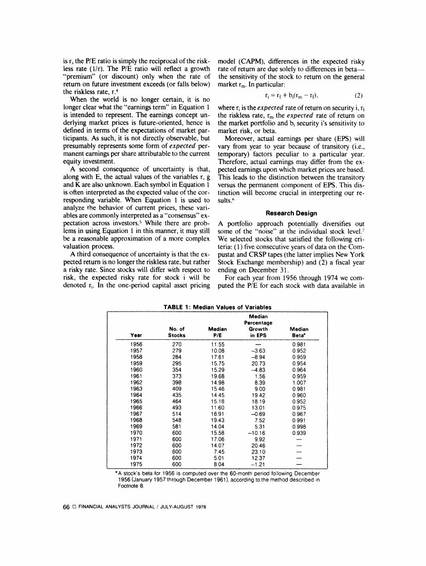
TABLE 1: Median Values of Variables

Median Percentage

No. of Median Growth Median Year Stocks P/E in EPS Beta*

1956 270 11.55 0.981 1957 279 10.08 -3.63 0.952 1958 284 17.61 -8.94 0.959 1959 295 15.75 20.73 0.954 1960 354 15.29 -4.83 0.964 1961 373 19.68 1.56 0.959 1962 398 14.98 8.39 1.007 1963 409 15.46 9.00 0.981 1964 435 14.45 19.42 0.960 1965 464 15.18 18.19 0.952 1966 493 11.60 13.01 0.975 1967 514 16.91 -0.69 0.967 1968 548 19.43 7.52 0.991 1969 581 14.04 5.31 0.998 1970 600 15.58 -10.16 0.939 1971 600 17.06 9.92 1972 600 14.07 20.46 1973 600 7.45 23.10 1974 600 5.01 12.37 1975 600 8.04 -1.21

*A stock's beta for 1956 is computed over the 60-month period following December 1956 (January 1957 through December 1961), according to the method described in Footnote 8.

66 O FINANCIAL ANALYSTS JOURNAL / JULY-AUGUST 1978

that year. We defined P/E as price per share on De- cember 31 divided by earnings per share for the year, computed on a pre-extraordinary item basis. Using data from the Compustat tape, we defined earnings growth as the percentage change in the year's earn- ings per share relative to the previous year and measured risk as the stock's beta, computed from monthly stock price return data available on the CRSP tape.8

We then ranked each year's stocks according to P/E and formed 25 portfolios, with Portfolio One comprising those four per cent with the highest P/E's and Portfolio 25 comprising the stocks with the lowest P/E's. We then compared the median P/E for each portfolio in its base year (year of formation) with the median P/E, median realized growth and median risk for the portfolio in subsequent years.9 Note that, in all cases, once formed the portfolio's composition was fixed (i.e., a buy and hold strategy was used).'0

Table 1 reports some summary statistics." Once a stock appears on the tape in a given year, its data are available from that year onward. The similarity of stocks appearing later relative to those appearing earlier is supported by the median beta, which shows no trend over time and is close to one. When we cor- related the median P/E for each year with the aggre- gate P/E ratio for Standard & Poor's Composite stocks for the years 1956 through 1975, we obtained a positive rank correlation of 0.85, which is reason- able, given the differences in the stocks and the methods used to compute the average P/E for a given year. Furthermore, the rank correlation between the

median annual growth rates reported in Table 1 and the growth in aggregate EPS for S&P Industrials yielded a positive correlation of 0.89.12

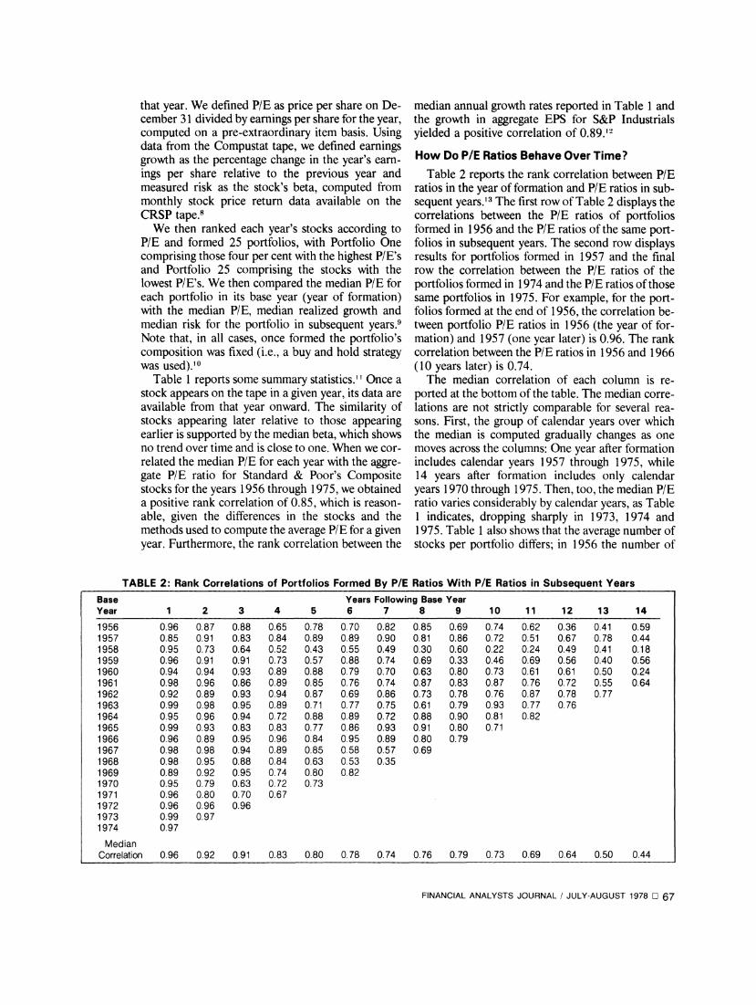
How Do P/E Ratios Behave Over Time? Table 2 reports the rank correlation between P/E

ratios in the year of formation and P/E ratios in sub- sequent years.'3 The first row of Table 2 displays the correlations between the P/E ratios of portfolios formed in 1956 and the P/E ratios of the same port- folios in subsequent years. The second row displays results for portfolios formed in 1957 and the final row the correlation between the P/E ratios of the portfolios formed in 1974 and the P/E ratios of those same portfolios in 1975. For example, for the port- folios formed at the end of 1956, the correlation be- tween portfolio P/E ratios in 1956 (the year of for- mation) and 1957 (one year later) is 0.96. The rank correlation between the P/E ratios in 1956 and 1966 (10 years later) is 0.74.

The median correlation of each column is re- ported at the bottom of the table. The median corre- lations are not strictly comparable for several rea- sons. First, the group of calendar years over which the median is computed gradually changes as one moves across the columns: One year after formation includes calendar years 1957 through 1975, while 14 years after formation includes only calendar years 1970 through 1975. Then, too, the median P/E ratio varies considerably by calendar years, as Table 1 indicates, dropping sharply in 1973, 1974 and 1975. Table 1 also shows that the average number of stocks per portfolio differs; in 1956 the number of

TABLE 2: Rank Correlations of Portfolios Formed By P/E Ratios With P/E Ratios in Subsequent Years

Base Years Following Base Year Year 1 2 3 4 5 6 7 8 9 10 11 12 13 14

1956 0.96 0.87 0.88 0.65 0.78 0.70 0.82 0.85 0.69 0.74 0.62 0.36 0.41 0.59 1957 0.85 0.91 0.83 0.84 0.89 0.89 0.90 0.81 0.86 0.72 0.51 0.67 0.78 0.44 1958 0.95 0.73 0.64 0.52 0.43 0.55 0.49 0.30 0.60 0.22 0.24 0.49 0.41 0.18 1959 0.96 0.91 0.91 0.73 0.57 0.88 0.74 0.69 0.33 0.46 0.69 0.56 0.40 0.56 1960 0.94 0.94 0.93 0.89 0.88 0.79 0.70 0.63 0.80 0.73 0.61 0.61 0.50 0.24 1961 0.98 0.96 0.86 0.89 0.85 0.76 0.74 0.87 0.83 0.87 0.76 0.72 0.55 0.64 1962 0.92 0.89 0.93 0.94 0.87 0.69 0.86 0.73 0.78 0.76 0.87 0.78 0.77 1963 0.99 0.98 0.95 0.89 0.71 0.77 0.75 0.61 0.79 0.93 0.77 0.76 1964 0.95 0.96 0.94 0.72 0.88 0.89 0.72 0.88 0.90 0.81 0.82 1965 0.99 0.93 0.83 0.83 0.77 0.86 0.93 0.91 0.80 0.71 1966 0.96 0.89 0.95 0.96 0.84 0.95 0.89 0.80 0.79 1967 0.98 0.98 0.94 0.89 0.85 0.58 0.57 0.69 1968 0.98 0.95 0.88 0.84 0.63 0.53 0.35 1969 0.89 0.92 0.95 0.74 0.80 0.82 1970 0.95 0.79 0.63 0.72 0.73 1971 0.96 0.80 0.70 0.67 1972 0.96 0.96 0.96 1973 0.99 0.97 1974 0.97

Median Correlation 0.96 0.92 0.91 0.83 0.80 0.78 0.74 0.76 0.79 0.73 0.69 0.64 0.50 0.44

FINANCIAL ANALYSTS JOURNAL / JULY-AUGUST 1978 L 67

stocks is 10, while the base years 1970 through 1974 average 24 per portfolio. On purely statistical grounds, the correlation coefficient should rise as the number of stocks per portfolio increases. How- ever, Table 2 does not display any obvious tendency for the correlations to increase systematically in the later base years.'4

With these caveats in mind, we interpret the correlations in Table 2 as supporting a long-term persistency in the portfolios' P/E ratios. With only two minor disruptions, the median correlation de- clines steadily with the number of years since port- folio formation. Five years after formation the me- dian correlation is 0.80, while 10 years after forma- tion the median correlation is 0.73. Fourteen years after formation, the median is 0.44. We tentatively conclude that, although much of the effect of the fac- tors that determine P/E ratios dissipates over the 14 years, a portion still clearly remains after five, 10 or perhaps even 14 years.

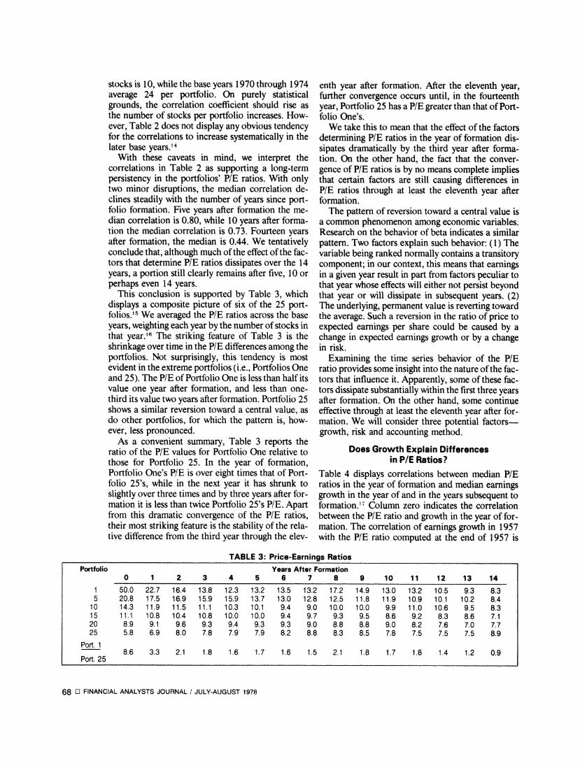
This conclusion is supported by Table 3, which displays a composite picture of six of the 25 port- folios.'5 We averaged the P/E ratios across the base years, weighting each year by the number of stocks in that year.'6 The striking feature of Table 3 is the shrinkage over time in the P/E differences among the portfolios. Not surprisingly, this tendency is most evident in the extreme portfolios (i.e., Portfolios One and 25). The P/E of Portfolio One is less than half its value one year after formation, and less than one- third its value two years after formation. Portfolio 25 shows a similar reversion toward a central value, as do other portfolios, for which the pattern is, how- ever, less pronounced.

As a convenient summary, Table 3 reports the ratio of the P/E values for Portfolio One relative to those for Portfolio 25. In the year of formation, Portfolio One's P/E is over eight times that of Port- folio 25's, while in the next year it has shrunk to slightly over three times and by three years after for- mation it is less than twice Portfolio 25's P/E. Apart from this dramatic convergence of the P/E ratios, their most striking feature is the stability of the rela- tive difference from the third year through the elev-

enth year after formation. After the eleventh year, further convergence occurs until, in the fourteenth year, Portfolio 25 has a P/E greater than that of Port- folio One's.

We take this to mean that the effect of the factors determining P/E ratios in the year of formation dis- sipates dramatically by the third year after forma- tion. On the other hand, the fact that the conver- gence of P/E ratios is by no means complete implies that certain factors are still causing differences in P/E ratios through at least the eleventh year after formation.

The pattern of reversion toward a central value is a common phenomenon among economic variables. Research on the behavior of beta indicates a similar pattern. Two factors explain such behavior: (1) The variable being ranked normally contains a transitory component; in our context, this means that earnings in a given year result in part from factors peculiar to that year whose effects will either not persist beyond that year or will dissipate in subsequent years. (2) The underlying, permanent value is reverting toward the average. Such a reversion in the ratio of price to expected earnings per share could be caused by a change in expected earnings growth or by a change in risk.

Examining the time series behavior of the P/E ratio provides some insight into the nature of the fac- tors that influence it. Apparently, some of these fac- tors dissipate substantially within the first three years after formation. On the other hand, some continue effective through at least the eleventh year after for- mation. We will consider three potential factors- growth, risk and accounting method.

Does Growth Explain Differences in P/E Ratios?

Table 4 displays correlations between median P/E ratios in the year of formation and median earnings growth in the year of and in the years subsequent to formation.'I Column zero indicates the correlation between the P/E ratio and growth in the year of for- mation. The correlation of earnings growth in 1957 with the P/E ratio computed at the end of 1957 is

TABLE 3: Price-Earnings Ratios Portfolio Years After Formation

0 1 2 3 4 5 6 7 8 9 10 11 12 13 14

1 50.0 22.7 16.4 13.8 12.3 13.2 13.5 13.2 17.2 14.9 13.0 13.2 10.5 9.3 8.3 5 20.8 17.5 16.9 15.9 15.9 13.7 13.0 12.8 12.5 11.8 11.9 10.9 10.1 10.2 8.4

10 14.3 11.9 11.5 11.1 10.3 10.1 9.4 9.0 10.0 10.0 9.9 11.0 10.6 9.5 8.3 15 11.1 10.8 10.4 10.8 10.0 10.0 9.4 9.7 9.3 9.5 8.6 9.2 8.3 8.6 7.1 20 8.9 9.1 9.6 9.3 9.4 9.3 9.3 9.0 8.8 8.8 9.0 8.2 7.6 7.0 7.7 25 5.8 6.9 8.0 7.8 7.9 7.9 8.2 8.8 8.3 8.5 7.8 7.5 7.5 7.5 8.9

Port. 1 8.6 3.3 2.1 1.8 1.6 1.7 1.6 1.5 2.1 1.8 1.7 1.8 1.4 1.2 0.9

Port. 25

68 O FINANCIAL ANALYSTS JOURNAL / JULY-AUGUST 1978

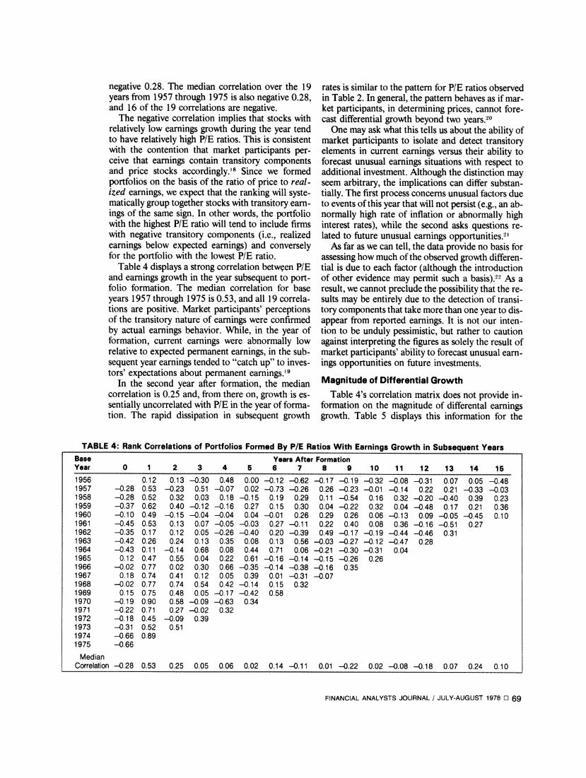
negative 0.28. The median correlation over the 19 years from 1957 through 1975 is also negative 0.28, and 16 of the 19 correlations are negative.

The negative correlation implies that stocks with relatively low earnings growth during the year tend to have relatively high P/E ratios. This is consistent with the contention that market participants per- ceive that earnings contain transitory components and price stocks accordingly.'8 Since we formed portfolios on the basis of the ratio of price to real- ized earnings, we expect that the ranking will syste- matically group together stocks with transitory earn- ings of the same sign. In other words, the portfolio with the highest P/E ratio will tend to include firms with negative transitory components (i.e., realized earnings below expected earnings) and conversely for the portfolio with the lowest P/E ratio.

Table 4 displays a strong correlation between P/E and earnings growth in the year subsequent to port- folio formation. The median correlation for base years 1957 through 1975 is 0.53, and all 19 correla- tions are positive. Market participants' perceptions of the transitory nature of earnings were confirmed by actual earnings behavior. While, in the year of formation, current earnings were abnormally low relative to expected permanent earnings, in the sub- sequent year earnings tended to "catch up" to inves- tors' expectations about permanent earnings.'9

In the second year after formation, the median correlation is 0.25 and, from there on, growth is es- sentially uncorrelated with P/E in the year of forma- tion. The rapid dissipation in subsequent growth

rates is similar to the pattern for P/E ratios observed in Table 2. In general, the pattern behaves as if mar- ket participants, in determining prices, cannot fore- cast differential growth beyond two years.20

One may ask what this tells us about the ability of market participants to isolate and detect transitory elements in current earnings versus their ability to forecast unusual earnings situations with respect to additional investment. Although the distinction may seem arbitrary, the implications can differ substan- tially. The first process concerns unusual factors due to events of this year that will not persist (e.g., an ab- normally high rate of inflation or abnormally high interest rates), while the second asks questions re- lated to future unusual earnings opportunities.2'

As far as we can tell, the data provide no basis for assessing how much of the observed growth differen- tial is due to each factor (although the introduction of other evidence may permit such a basis).2' As a result, we cannot preclude the possibility that the re- sults may be entirely due to the detection of transi- tory components that take more than one year to dis- appear from reported earnings. It is not our inten- tion to be unduly pessimistic, but rather to caution against interpreting the figures as solely the result of market participants' ability to forecast unusual earn- ings opportunities on future investments.

Magnitude of Differential Growth Table 4's correlation matrix does not provide in-

formation on the magnitude of differental earnings growth. Table 5 displays this information for the

TABLE 4: Rank Correlations of Portfolios Formed By P/E Ratios With Earnings Growth in Subsequent Years Base Years After Formation Year 0 1 2 3 4 5 6 7 8 9 10 11 12 13 14 15

1956 0.12 0.13 -0.30 0.48 0.00 -0.12 -0.62 -0.17 -0.19 -0.32 -0.08 -0.31 0.07 0.05 -0.48 1957 -0.28 0.53 -0.23 0.51 -0.07 0.02 -0.73 -0.26 0.26 -0.23 -0.01 -0.14 0.22 0.21 -0.33 -0.03 1958 -0.28 0.52 0.32 0.03 0.18 -0.15 0.19 0.29 0.11 -0.54 0.16 0.32 -0.20 -0.40 0.39 0.23 1959 -0.37 0.62 0.40 -0.12 -0.16 0.27 0.15 0.30 0.04 -0.22 0.32 0.04 -0.48 0.17 0.21 0.36 1960 -0.10 0.49 -0.15 -0.04 -0.04 0.04 -0.01 0.26 0.29 0.26 0.06 -0.13 0.09 -0.05 -0.45 0.10 1961 -0.45 0.53 0.13 0.07 -0.05 -0.03 0.27 -0.11 0.22 0.40 0.08 0.36 -0.16 -0.51 0.27 1962 -0.35 0.17 0.12 0.05 -0.26 -0.40 0.20 -0.39 0.49 -0.17 -0.19 -0.44 -0.46 0.31 1963 -0.42 0.26 0.24 0.13 0.35 0.08 0.13 0.56 -0.03 -0.27 -0.12 -0.47 0.28 1964 -0.43 0.11 -0.14 0.68 0.08 0.44 0.71 0.06 -0.21 -0.30 -0.31 0.04 1965 0.12 0.47 0.55 0.04 0.22 0.61 -0.16 -0.14 -0.15 -0.26 0.26 1966 -0.02 0.77 0.02 0.30 0.66 -0.35 -0.14 -0.38 -0.16 0.35 1967 0.18 0.74 0.41 0.12 0.05 0.39 0.01 -0.31 -0.07 1968 -0.02 0.77 0.74 0.54 0.42 -0.14 0.15 0.32 1969 0.15 0.75 0.48 0.05 -0.17 -0.42 0.58 1970 -0.19 0.90 0.58 -0.09 -0.63 0.34 1971 -0.22 0.71 0.27 -0.02 0.32 1972 -0.18 0.45 -0.09 0.39 1973 -0.31 0.52 0.51 1974 -0.66 0.89 1975 -0.66

Median Correlation -0.28 0.53 0.25 0.05 0.06 0.02 0.14 -0.11 0.01 -0.22 0.02 -0.08 -0.18 0.07 0.24 0.10

FINANCIAL ANALYSTS JOURNAL / JULY-AUGUST 1978 E 69

same six composite portfolios reported in Table 3, using the same composite process. The results sup- port the contentions made earlier. Portfolio One (the highest P/E portfolio) experienced a median drop in earnings of 4.1 per cent, while Portfolio 25 experi- enced a median earnings increase of 26.4 per cent. In simplest terms, the prices of the stocks in Port- folio One did not change proportionately with their earnings; as a result, their P/E ratios were relatively high. Similarly, the stocks in Portfolio 25 experi- enced a price change that, on average, was less than 26 per cent, and their P/E ratios were relatively low. Again, this implies a price formation process whereby participants view changes in earnings as containing a transitory element.

In Table 5, Portfolio One shows a median earn- ings growth of 95.3 per cent in the first year after for- mation, while Portfolio 25 shows a drop in earnings of 3.3 per cent. This is consistent with the results re- ported in Table 4: The perceptions of market partic- ipants regarding the transitory element in earnings were confirmed by subsequent earnings behavior.

The results in Table 5 differ from those in Table 4 in one major respect-the highest P/E portfolio maintains its distinctive earnings growth behavior for seven years after formation. This is neither con- tradictory nor surprising. Whereas correlations in Table 4 reflect the strength of the relationship for all 25 portfolios, where growth and P/E are essentially unrelated after two years, the comparison described above involves only one of those portfolios. For that one " extreme" portfolio we would expect non- normal growth to be larger and to last longer.

The results in Table 5 can be deceptive in at least two respects. First, they reflect the average effect across a number of base years and do not reveal variation from one base year to another. A more detailed examination, not reported here, revealed considerable variation across base years. Second, while it is intuitively appealing to focus solely on the high P/E portfolio, it constitutes only four per cent of the observations. It is important to remember that, with the remaining portfolios included, there is little or no apparent relation beyond the second year.

Comparing the P/E analysis with the growth analysis, we conclude that some of the initial dissipa- tion of the P/E ratio in the first three years after for- mation can be explained by differential growth in earnings. Beyond that, however, there clearly exists a P/E differential that cannot be explained by differ- ential earnings growth.

Before leaving growth analysis, we'd like to com- ment on one aspect of the data. In contrast to P/E ratios, which exhibit a high degree of correlation over time, previous evidence indicates that earnings growth rates possess near-zero correlation over time. To ensure that the same behavior held for the stocks in our sample, we constructed a portfolio strategy based on earnings growth in the year of formation and then observed subsequent growth. Our results confirmed previous findings of near-zero correlation of earnings growth rates. While a mechanical process relying on past growth rates is largely unsuccessful in predicting future differential growth, the P/E ratio is successful because price reflects a process whereby market participants rely on more information than past earnings in distinguishing the transitory and permanent components of earnings.

Risk Analysis

The expected sign of the correlation between P/E and beta may be either positive or negative. The ar- gument is developed in greater detail in the appen- dix, but it essentially proceeds as follows: Stocks' earnings move together because of economy-wide factors. In years of transitorily low earnings, the market-wide P/E will tend to be high, but stocks with high betas will tend to have even higher P/E ratios because their earnings are most sensitive to econ- omy-wide events. Conversely, in years of transitorily high earnings, high beta stocks will have even lower P/E ratios than most. Therefore we expect a positive correlation in "high" P/E years and a negative corre- lation in "low" years.

Table 6 reports the rank correlations between P/E and beta. We compared beta for a given base year over the 60 months subsequent to formation; thus the beta for 1956 was computed over the years 1957

TABLE 5: Earnings Growth

Portfolio Years After Formation 0 1 2 3 4 5 6 7 8 9 10 11 12 13 14

1 -4.1 95.3 37.2 28.2 16.4 18.9 18.1 19.7 13.1 14.8 15.3 10.8 10.9 10.2 11.8 5 10.7 14.9 12.1 13.1 14.2 10.9 10.4 11.8 10.5 11.6 8.0 11.9 8.3 13.3 18.1

10 9.6 12.9 11.5 12.3 12.6 9.2 10.1 10.8 12.8 8.3 12.9 22.2 16.6 20.6 29.6 15 10.0 8.8 8.5 8.1 8.2 14.3 11.6 5.4 13.3 10.3 11.0 10.8 11.9 12.8 33.4 20 10.8 5.2 9.3 12.6 12.4 6.0 8.4 13.0 10.2 11.3 11.1 25.0 12.9 17.7 18.0 25 26.4 -3.3 7.5 10.8 8.3 12.9 17.1 13.6 18.0 12.8 16.7 14.2 10.9 12.4 10.1

Port. 1 -0.155 * 5.0 2.61 1.98 1.47 1.06 1.45 0.73 1.16 0.92 0.76 1.00 0.82 1.17

Port. 25

*Not meaningful because of negative growth in denominator.

70 D FINANCIAL ANALYSTS JOURNAL / JULY-AUGUST 1978

TABLE 6: Rank Correlations of Portfolio Median P/E Ratios and Median Beta

Rank of Predicted Rank Median Sign of

Year Correlation P/Es Correlation

1956 -0.34 14 -

1957 -0.23 15 -

1958 0.22 3 + 1959 0.41 5 + 1960 0.50 8 + 1961 0.55 1 + 1962 -0.48 10 -

1963 -0.42 7 + b

1964 -0.63 11 -

1965 -0.26 9 -

1966 -0.44 13 -

1967 0.50 4 + 1968 0.53 2 + 1969 0.58 12 _b 1970 0.28 6 +

Median Adjusted for Predicted 0.41

Sign a Computed from Table 1. b 1963 and 1969 are the two years incorrectly predicted.

through 1961. To predict the sign of the correlation in a given

base year, we ranked the market-wide P/E ratios (as reported in Table 1) from high to low.23 We hy- pothesized that the years with the eight highest values of market-wide P/E ratios would have a posi- tive correlation between P/E and beta, while the years with the seven lowest values of market-wide P/E would have a negative correlation. Over the 15 base years 1956 through 1970, the actual correla- tions are positive eight times and negative seven times. We correctly predicted the sign of the correla- tion for 13 of the 15 years. This is impressive, given the crudeness of the test. (The test's limitations are discussed in the appendix.)

Table 7 reports the magnitude of the betas for the six portfolios presented in Tables 3 and 5. Because the relation between P/E and beta can be either posi- tive or negative, we averaged results over two sets of years-those in which the correlation was positive

Table 7: Relation of P/E and Beta

Average Average Beta Beta

Average in Years of in Years of Beta in Positive Negative

Portfolio All Years Correlation Correlation

1 1.22 1.28 1.13 5 1.01 1.03 0.98

10 1.05 1.09 1.00 15 0.96 0.94 1.00 20 1.03 0.96 1.11 25 1.04 0.95 1.14

and those in which the correlation was negative. The third column reports the beta differences for the years of positive correlation. The differences are small for Portfolios Five through 25, where beta ranges from 1.09 to 0.94. The largest difference oc- curs in the highest P/E portfolio, with its beta of 1.28. In the fourth column, negative correlation is evident for Portfolios Five through 25, with a pro- nounced aberrant behavior for Portfolio One. For this set of stocks, a "U-shaped" relationship is pres- ent. Given the consistently high betas of the highest P/E portfolio, it is imperative that some form of risk- adjusted performance standard be introduced to avoid spuriously inferring superior stock price per- formance.

While beta clearly holds some explanatory power, the crucial issue is, to what extent does it explain the P/E ratio behavior reported in Tables 2 and 3? We think it explains little: If beta were an important ex- planatory variable, then the predicted behavior of P/E over time would be much different from what Tables 2 and 3 report. Stocks in Portfolio One dur- ing years of high market-wide P/E would tend to move to Portfolio 25 (or its neighbors) in years of low market-wide P/E. Looking across a row of Table 2, we would expect to see a pattern of positive and negative correlations similar to that reported in the last column of Table 6. Instead, we observe a strong positive serial correlation throughout.24 Further- more, the relative differences in betas are not of the same magnitude as the relative differences in P/E ratios. Before considering another source of P/E dif- ferences, however, we report the results of a regres- sion analysis that combines both growth and risk analysis.

Regression Analysis

Table 8 displays the results of a simple linear re- gression that included beta and earnings growth as independent variables. We used the EIP, rather than P/E, ratio because the Litzenberger and Rao model posits linearity in E/P (not in P/E).25 The expected sign of the E/P and beta relationship is thus the re- verse of that shown in the final column of Table 6. The actual regression coefficients have the predicted sign in 13 of the 15 years; again, 1963 and 1969 are exceptions.

The predicted signs of the growth coefficients are also negative, since we're using E/P as the dependent variable. For growth in the year subsequent to port- folio formation (gl), all 15 coefficients have the pre- dicted sign. Growth two years subsequent to forma- tion (g2) has the predicted sign in 12 years. By the third year (g3), however, the signs of the coefficients are evenly divided. Table 4 suggests there is little merit to introducing additional growth variables.

FINANCIAL ANALYSTS JOURNAL I JULY-AUGUST 1978 O 71

TABLE 8: E/P Regression Results

Regression Coefficients Adjusted F (t-Statistic) R2 Statistic

Base Year Constant Beta 91 92 93

1956 0.070 0.030 --0.046 -0.035 0.053 01523 1956 0.070 (0.71) (-1.38) (-0.73) (0.93) 0.185 2.36

1957 0.348 0.086* -0. 142' -0.066 -0.1 23' .8 .( 1957 0.348 (1.74) (-4.13) (-1.57) (-2.29) 0.581 930*

1958 0.136 0000 -0.01 9) -0.070 0.013 0.270 3.96 (0) (-2.57) (-1.69) (0.26)

1959 0.076 -0.053' -0.157* 0.098 0.086 0.505 7.13* (-1.76) (-4.45) (1.29) (1.62)

1960 0.155 -0.075* -0. 1 61'* 0.046 0.092 0.502 7.06* 1960 0.155 ~~(-2.83) (-3.55) (0.71) (1.17) 0.2706

1961 0.077 -0.054* -0.063 0.064 0.023 0.289 3.44* (-1.89) (-1.25) (0.93) (0.57)

1962 0.119 0.1 16* --0.055' -0.026 --0.064 0.524 7.61* (4.68) (-2.10) (-0.50) (-1.02)

1963 0239 0. 09 7* -0. 106* -0.089' -0.034 037452 1963 0.239 (3.10) (-1.93) (-1.84) (-0.62) 0370 4.52*

1964 0.260 0. 0076* -0.085 -0.045 -0 114' 0.572 9.03* 1964 0.260

~~(2.36) (-1.26) (-0.67) (-2.24) 0.7903

1965 0.300 0.071* -0. 167* -0.091' -0-022 047644 1965 0.300 ?(2.00) (-2.54) (-1.73) (-0.32) 0.475 6.44*

1966 0.501 0. 112' -0.304' -0.068 -0. 138* 0.783 22.63* (3.53) (-7.06) (-0.96) (-1.80)

1967 0.447 -0.065* -0. 164' -0.106 --0034 05791, 1967 0.447 (_-2.15) (-2.87) (-1.67) (-0.94) 0.575 9.10'

1968 0.285 -0.031 -0.033 -0. 108; -0.060 0.738 17.91* (-1.71) (-1.71) (-5.23) (-1.62)

-0.054 -0. 159' -0. 134' 0.030 1969 0.380 (-1.40) (-4.64) (-2.09) (0.57) 0.658 12.56*

1970 0.185 -0.029 -0.003 -0. 1 67* 0.089 0.391 4.86* (-0.71) (-0.28) (-2.58) (1.42)

*Significant at five per cent level (one-tail test on regression coeff icients).

The R2 (proportion of variance explained) adjusted for degrees of freedom ranges from 18.5 per cent to 78.3 per cent, with a median of 50.5 per cent. The F- statistic, which tests the null hypothesis that all of the coefficients ate zero, is significant at the five per cent level in 13 of the 15 years."'i

While risk and growth on the average explain ap- proximately 50 per cent of the variance of the EIP ratio, they obviously leave an equal proportion un- explained. Thus the regression results presented in Table 8 provide only the crude beginnings of an at- tempt to explain cross-sectional P/E differences. We suggest further research in a number of areas: (1) Even if the realized values of beta and growth are unbiased estimates of expectations, they may still measure those expectations with error; better speci- fication could lead to higher R2, which is under-

stated when measurement error is present. (2) Better specification of the denominator of the P/E ratio might yield better results. ' (3) Accounting rules could be creating P/E differences; our final com- ments are devoted to this area.

Accounting Method

The finding that P/E ratio differences persist well beyond three years after portfolio formation suggests the influence of some factor other than risk or growth. Accounting effects are obvious candidates. Accounting method effects are of two types- use of different rules (e.g., depreciation methods) by differ- ent firms for essentially the same or similar circum- stances and errors introduced by applying a uniform accounting rule (e.g., historical cost) to differing

72 O FINANCIAL ANALYSTS JOURNAL / JULY-AUGUST 1978

economic circumstances (e.g., current value of assets).

The P/E ratio will be influenced by the effect on earnings of differing accounting methods. Assuming prices are not dependent on the accounting method used in annual reports, firms that use conservative accounting methods (e.g., accelerated depreciation or LIFO inventory valuation) would tend to have higher P/E ratios than firms that use less conserva- tive methods, holding constant the effects of risk and growth.'8 For example, Beaver and Dukes found the P/E ratios of a portfolio of firms using accelerated depreciation were greater than the P/E ratios of a portfolio of firms using straight-line depreciation.'9 The two portfolios were essentially the same with respect to risk (beta) and growth. Moreover, when the earnings of the straight-line portfolio were con- verted according to the accelerated method, the P/E ratios were essentially the same for both portfolios. In other words, the P/E differences in the two port- folios disappeared when earnings were computed on a uniform depreciation method. We suggest an ex- tension of this type of analysis to other accounting methods as an obvious candidate for future re- search.30 U

APPENDIX

If the EPS used to compute P/E ratios contained no transitory elements, we would expect a positive rela- tion between E/P and beta and a negative relation between P/E and beta. However, the evidence sug- gests that transitory elements in EPS are present. How does this affect the analysis of risk?

Previous empirical research indicates that a stock's E/P ratio can be characterized by the follow- ing (linear) process:

E/Pt=a+bMt+ut (a)

where E/Pt = earnings-price ratio for a stock in year t,

Mt = a market-wide E/P ratio for year t,

ut = a non-market residual for a stock in year tand

= the intercept and slope of the linear 6 } , relationship.

Moreover, this research has shown that, at the port- folio level, b (the earnings-price "beta") is highly correlated with beta.

In a given year where the actual, realized earnings may differ from the expected earnings, what relation can we expect between E/P and beta? Rearranging

(a) we have:

(E/Pt - E/P) = b(Mt - M) + Ut (b)

where E/P = expected value of E/Pt and M = expected value of Mt

Ignoring ut and taking b equal to b, we have:

(E/Pt - E/P) = b(Mt - M) . (c)

When the realized Mt is above its expected value, stocks with higher betas will have higher E/P's (ex- pressed as a deviation from the expected value). However, when the realized M1 is below its expected value, stocks with higher betas will have lower E/P's (expressed in terms of a deviation from its mean).

Limitations of the Empirical Test

One obvious limitation is the failure to express P/E (or E/P) as a deviation from its expected value, as indicated by Equation (c). This test implicitly assumes that inter-stock P/E differences are zero. This is obviously not the case, as Tables 2 and 3 in- dicate. However, we did not take this latter step since our concern throughout has been with the risk differences of a simple, P/E-oriented portfolio strategy, not a strategy that expresses P/E as a devia- tion from its expected value. A second limitation is the assumption that 15 years taken as a whole con- tain approximately an equal number of realizations above and below the expected value, which in turn is assumed to be a constant over 15 years.

In the absence of any other evidence, this assump- tion seems as reasonable as any other. However, the assumption of a constant expected value cannot be strictly true. Factors such as changing interest rates would lead us to expect that market-wide P/E ratios change over time. Third, the test ignores the influ- ence of ut (the unsystematic component) as ex- pressed in Equation (b).

Further Analysis of Table 7

Evidence in our article supports the contention that transitory elements in earnings exist. We would expect high P/E stocks to have greater earnings vari- ability to the extent that transitory elements account for P/E differences. Research by Beaver and Mane- gold, among others, confirms that stocks with greater earnings variability have higher betas. However, the argument is not complete: If earnings volatility were exclusively systematic, we would have observed no U-shaped behavior in the years with negative corre- lation. If unsystematic earnings volatility (the vari- ance of ut from Equation (a) ) is positively correlated with beta, and if high P/E stocks have greater unsys- tematic volatility, the result would be a consistently higher beta for the highest P/E portfolio. However, a

FINANCIAL ANALYSTS JOURNAL / JULY-AUGUST 1978 FO 73

similar argument could be offered for the lowest P/E portfolio. Yet consistently higher betas are not ob- served here. We offer no explanation for this result.

Footnotes 1. See I. Little, "Higgledy Piggledy Growth" (Institute

of Statistics, Oxford, November 1962), the seminal work. See also R. Ball and R. Watts, "Some Time Series Properties of Accounting Earnings Numbers," Journal of Finance (June 1972), pp. 663-682; J. Cragg and B. Malkiel, "The Consensus and Accuracy of Some Predictions of the Growth of Corporate Earnings," Journal of Finance (March 1968), pp. 67-84; I. Little and Raynor, Higgledy Piggledy Growth Again (Oxford: Basil Blackwell, 1966); and J. Murphy, "Relative Growth in Earnings Per Share-Past and Future," Financial Analysts Jour- nal (November/December 1966), pp. 73-76. Excel- lent summaries appear in R. Brealey, An Introduc- tion to Risk and Return from Common Stocks (Cambridge: MIT Press, 1969) and in J. Lorie and M. Hamilton, The Stock Market: Theories and Evi- dence (Homewood, Illinois: Irwin, 1973).

2. Previous studies have attempted to use the P/E ratio itself as a growth predictor-with little success. Two examples are Cragg and Malkiel, "Consensus and Accuracy" and J. Murphy and H. Stevenson, "Price/Earnings Ratios and Future Growth of Earn- ings and Dividends," Financial Analysts Journal (November/December 1967), pp. 1 11- 1 14. The port- folio strategy adopted in our study provides an op- portunity to uncover relations that may have been undetected by previous research.

3. Let CFt equal the cash flow generated t periods from now from current equity investment. Assuming r is constant:

E xc r CFt (1 + r)-t = Present Value of Current r 1 Equity Investment,

E r l CFt (I + r)A-t =Permanent , t= I Earnings

4 It appears to us that a basic inconsistency may exist when perfect markets are invoked to motivate present value formulas and yet abnormal returns in produc- tive opportunities are posited to explain growth pre- miums or discounts in P/E ratios. However, this is a puzzle we are not prepared to resolve. Stocks may still be priced "as if' a discounted cash flow model were applied even in the presence of abnormal returns in the productive sector (i.e., the product and factor markets).

5. Consensus expectations in general depend on the wealth, risk preferences and beliefs of market partici- pants. ("Market participants" is a generic term in- tended to include individuals whose expectations di- rectly or indirectly influence market prices-i.e., analysts as well as investors.) In a one-period setting, expressing price as a function of expected values is an

arbitrary, although innoucuous, way to view valua- tion. In a multi-period setting, however, such a valua- tion scheme will not necessarily hold.

6. Previous attempts by researchers to remove transitory elements from earnings vary from subjective adjust- ments of the components of earnings to statistical data fitting via Box-Jenkins techniques. For an exam- ple of the latter, see P. Griffin, "The Time Series Be- havior of Quarterly Earnings," Journal of Account- ing Research (Spring 1977), 71-83.

We would like to be able to say a portfolio ap- proach will permit us to diversify out the transitory earnings components. Clearly we cannot make such a statement. To the contrary, since the portfolios will be formed on the basis of the ratio of price to real- ized earnings, we expect the ranking will systemati- cally group together stocks with transitory earnings of the same sign. In other words, the portfolio with the highest P/E ratios will tend to include firms where the transitory component is negative (i.e., realized earn- ings are below expected earnings) and conversely for the portfolio with the lowest P/E ratios. Our evidence will support these contentions, and it is a major point to keep in mind in interpreting the results.

7. For a more detailed discussion of the effects of aggre- gation into portfolios see W. Beaver and J. Mane- gold, "The Association Between Market-Determined and Accounting-Determined Risk Measures," Jour- nal of Financial and Quantitative Analysis (June 1975), pp. 231-284. In this context, "noise" refers to the fact that our growth and risk measures may differ from the growth and risk expected at the time of port- folio formation.

8. Beta was estimated as the slope of a linear regression of the form:

Rit = ai + biRmt + eit , t = 1,60

where Rit equals monthly percentage change in price (adjusted for dividends) for security i in month t and Rmt equals monthly percentage change in a market index of price changes (adjusted for dividends) of all NYSE firms (provided as part of CRSP tape).

9. The median was used because it was a nonparametric measure that would place less demands on the data. Various weighting schemes (e.g., weighting by market value) were also applied with essentially the same re- sults as reported here. Since it is unclear how to de- fine growth off of negative earnings, the portfolios were formed only over those stocks with positive earnings in the base year. However, the sign of earn- ings was unrestricted in the years subsequent to for- mation. Hence earnings could be negative in later years.

10. The Compustat tape contains those firms that have survived mergers and bankruptcy. We would expect that this could induce a potential bias in the levels of the variables to be studied. However, the study focuses on differences in these variables across port- folios of stocks. It is not obvious to what extent sur- vivorship imparts a bias for this purpose. This would require knowledge of how non-surviving firms sys-

74 O FINANCIAL ANALYSTS JOURNAL / JULY-AUGUST 1978

tematically differ from surviving ones. In any event, because of the survivorship criteria, the portfolio strategies described here could not have been literally followed by an investor.

11. The number of stocks increases over time because of availability on the Compustat tape. In virtually all in- stances, the firms with incomplete histories on Com- pustat existed throughout the 1956-75 period but were picked up at some later date by Compustat. In other words, the firms being added do not tend to be new firms.

12. These aggregate statistics were obtained from S&P's Trade and Securities Statistics, 1976.

13. It is important to realize that a correlation matrix like that of Table 2 invariably leaves out certain informa- tion. For example, does a correlation coefficient of one mean the P/E difference between portfolios re- mains approximately the same as it was in the year of formation? Not necessarily. We can draw no infer- ence about the magnitude of portfolio differences; the rank correlation coefficient merely indicates a similarity in the rankings of the portfolios. A coeffi- cient of one indicates that the rankings of two port- folios remain the same, but it does not tell us any- thing about the spread between the portfolios. The spread between the portfolios may have shrunk or grown. However, we do know that, even if the spread has changed, at least the relative positions remained unaltered.

14. Since the P/E ratios are highly correlated, we cannot view elements in one cell as unrelated to the other cells; the results in two adjacent rows should be high- ly related. In other words, the results for the base year 1957 are, not surprisingly, similar to the results for the base year 1956. Because the results are not per- fectly correlated, however, some additional informa- tion is conveyed by repeating the portfolio strategy for different base years.

15. Table 3 is subject to the same caveats as Table 2. For example, the years 1971 through 1975 play a rela- tively more important role in the later years after for- mation, so the P/E ratios exhibit a downward drift. The real focal point of the table is the difference in P/E ratios across portfolios, rather than the common movement by all portfolios. Moreover, the results of a more extensive examination of the data, which held constant the calendar year composition of each year, did not differ from the findings shown in Table 3. We chose Table 3's composite because it was the most comprehensive and the simplest method of presenta- tion.

16. For example, for Year 0 (the year of formation), the average P/E ratio for Portfolio One was computed by taking a weighted average of each of the median P/E ratios for Portfolio One for the years 1956-74 inclu- sive. The weights were determined by the number of securities in that portfolio in that year. 1956, with 10 securities per portfolio, carried a weight of 0.029, while 1970-74 carried weights of 0.070 each with the sum of the weights over the 1956-74 period equalling one.

17. Since earnings could be negative in any subsequent

year, a problem rose as to how to define growth when the denominator is negative. When earnings changed from negative to positive, the growth was defined to be greater than the median (i.e., "very large"). When earnings remained negative in both years, the obser- vation was deleted. Typically, this caused a deletion of less than two per cent of the observations, with the exception of Portfolio One, where deletions ranged from two to three per cent of the observations.

18. We regard the transitory earnings argument as one, but by no means the only, interpretation to place on the results.

19. Suppose expected earnings per share are $1.00. For convenience, assume that realized earnings per share were $1.00 and $0.75 in 19xl and 19x2. The actual growth rate of 19x2 is -25 per cent, while the ex- pected growth in 19x3 is 33 per cent. Assuming price remains essentially unchanged (because permanent earnings are unchanged) at $10.00, the P/E ratio would be 10 and 13.3 for 19xl and 19x2, while the expected P/E in 1 9x3 would be 10. Note that in 1 9x2 there was an abnormal low earnings growth asso- ciated with a high P/E (negative correlation) and that a high P/E in l9x2 was followed by abnormal high growth in l9x3 (positive correlation). This is dis- cussed in more detail in W. Beaver, "The Informa- tion Content of the Magnitude of Unexpected Earn- ings" (Stanford Research Seminar, 1974).

20. This conclusion is contingent upon the way we chose to measure the variables and to rank the portfolios. For example, a longer term measure of growth (i.e., five or 10 years) might produce different results.

21. By unusual earnings opportunities we essentially mean opportunities to earn a return on future invest- ments greater than the cost of capital. Valuation theory tells us that this form of future earnings growth will induce a growth premium in the P/E. Note that it is crucial to distinguish between unusual earnings op- portunities on future, rather than current, invest- ment. To the extent there are abnormal returns earned on the current investment, this will not affect the P/E ratio, although the ratio of market price to book value per share would be affected.

22. For example, if one believes that product and factor markets are reasonably competitive, then there exist little or no unusual earnings opportunities and the observed growth differences are almost entirely due to transitory factors.

23. Operationally, the market-wide P/E was defined to be the median P/E as reported in Table 1.

24. Although not reported here, the analysis of the serial correlation in P/E behavior was augmented by an analysis of a transition matrix. This analysis also con- firmed the lack of any material tendency to move from one extreme portfolio to extreme portfolios at the other end of the P/E spectrum.

25. Since our study is concerned with differences across P/E ratios at a given point in time, beta (bi) will be the sole determinant of differences in P/E resulting from differences in ri. Assuming a finite growth horizon, Litzenberger and Rao ("Estimates of the Marginal Rate of Time Preference and Average Risk Aversion

FINANCIAL ANALYSTS JOURNAL / JULY-AUGUST 1978 a 75

of Investors in Electric Utility Shares: 1960-66," The Bell Journal of Economics and Management Science (Spring 1971), pp. 265-277) have shown the E/P ratio (the reciprocal of P/E) is a simple linear function of beta and a growth variable, with the fol- lowing form:

l=Yo+ 'Ylbl =Y2f(g)

Pi

The sign of yI is expected to vary, f(g) is some func- tion of growth and Y2 is expected to be negative.

26. An analysis of the residuals indicated that they are well approximated by normality. This is not sur- prising in the sense that each observation is an "average" for a portfolio of stocks. By the Central Limit Theorem, we would expect the sampling distri- butions of averages to approach normality. Note, however, that the results from any one year's regres- sion are not independent of those of other years.

27. Two approaches immediately come to mind-the ap- plication of Box-Jenkins techniques to the past earn- ings series or the use of analysts' forecasts of earnings. Either method might produce better assessments of expected earnings per share.

28. This ordinal statement holds for both depreciation and inventory, even though inventory also implies a "real" difference due to taxes. Obviously, the specific adjustments to be made would have to distinguish be- tween accounting differences that imply tax differ- ences versus those that do not.

29. W. Beaver and R. Dukes, "Delta-Depreciation Methods: Some Empirical Results," Accounting Review (April 1972), pp. 320-332. In this study, all sample firms were using an accelerated method for tax purposes. Therefore the difference was solely due to the depreciation method used for annual report purposes.

30. Another approach would be to introduce variables related to the accounting effect. Recent works by Watts and Zimmerman ("Toward a Positive Theory of the Determination of Accounting Standards," Ac- counting Review (April 1978) ) suggest that conser- vativeness of accounting method varies positively with firm size. Van Breda ("The Prediction of Corpo- rate Earnings" (Stanford University, 1976)) indi- cates that average age of assets is one of the variables that explains cross-sectional differences in return on equity (i.e., earnings available to common dividend by the book value of common equity).

Securities

and Regulation continued from page 38

"... the Metcalf hearings conveyed one very definite and clear message- a sense of expectation and urgency for the profes- sion and, as necessary, the Commission, to act to build the public's confidence in the independence of accountants, in their resolve and ability to engage in meaning- ful self-discipline, and in the process by which accounting standards are estab- lished.

"I have very little desire to preside, during my five years as Chairman, over increased regulation of the accounting profession. Similarly, I have no wish to see legislation passed that would place the responsibility on the Commission-or some other government body-to regu- late accountants. Nevertheless, time is rapidly running out on the opportunity for voluntary initiatives."

In fact, the Metcalf Subcommittee's

recommendations, issued on Novem- ber 14, 1977, involved much less far- reaching federal intervention than the January 1977 staff report recom- mended. The subcommittee report on "Improving the Accountability of Publicly-Owned Corporations and their Auditors" recommended con- tinued emphasis on self-regulation for accountants and the establishment of a self-regulatory organization, possi- bly with mandatory membership, sub- ject to SEC oversight. The report con- cluded that the accounting profession and the SEC should "act in a timely manner to implement the policy goals in this report."

However, Representative Moss, Chairman of the House Subcom- mittee on Oversight and Investiga- tions, speaking in early March 1978, warned the accounting profession that he would seek legislation to impose federal regulation of accountants un- less the accounting profession im- proved its self-regulatory efforts. Moss seemed particularly concerned about the possible anti-competitive

aspects of the new AICPA self-regu- latory program. Although Moss is rumored to be on the verge of intro- ducing a new bill, he has indicated that he would not seek re-election.

AICPA Actions

In September 1977, the Council of the AICPA adopted a proposal to create a new division of CPA firms that would comprise two sections with voluntary firm membership-the SEC Practice section, for CPA firms whose clients are SEC registrants, and the Private Companies Practice sec- tion, for firms serving companies not registered with the SEC. (A firm could be a member of both sections.) Each section would be administered by a 21 -member executive committee.

A five-member Public Oversight Board will have power to monitor ac- tivities of the SEC Practice section and report its findings publicly. It could also impose sanctions such as requiring a firm to take internal ac- tion to improve its controls or opera-

concluded on page 85

76 O FINANCIAL ANALYSTS JOURNAL / JULY-AUGUST 1978