What could not be in Feynman lectures:

Bell inequalities

V. Cerny

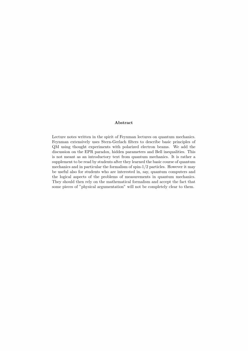
Abstract

Lecture notes written in the spirit of Feynman lectures on quantum mechanics.Feynman extensively uses Stern-Gerlach filters to describe basic principles ofQM using thought experiments with polarized electron beams. We add thediscussion on the EPR paradox, hidden parameters and Bell inequalities. Thisis not meant as an introductory text from quantum mechanics. It is rather asupplement to be read by students after they learned the basic course of quantummechanics and in particular the formalism of spin-1/2 particles. However it maybe useful also for students who are interested in, say, quantum computers andthe logical aspects of the problems of measurements in quantum mechanics.They should then rely on the mathematical formalism and accept the fact thatsome pieces of ”physical argumentation” will not be completely clear to them.

1 Stern Gerlach filters

In this section we briefly repeat what was (at least ”in spirit”) written in theFeynman lectures. We shall speak on beams of electrons passing through variousStern Gerlach filters. This kind of language has only symbolical meaning. Wedo not care whether the described experiments are really technically feasible.We use the philosophy of the thought experiments heavily exploited by Einstein,Bohr and Feynman. Thought experiments are performed virtually, just in ourimagination. There might be technical problems if we tried to perform them inreality. However we carefully check that on a principal level there is nothing toprevent them working. The principal components used in our experiments willbe an electron gun producing a beam of unpolarized electrons, Stern Gerlachfilters and electron detectors which detect electrons with ideal efficiency irre-spective of their polarization. Electrons are fermions with spin 1/2. Their spinstates are described by vectors in two-dimensional Hilbert space. A base in theHilbert space can be chosen arbitrarily: most often one chooses the base formedby the eigenstates of the operator of the projection of the spin to the z-axis. Wshall denote these base vectors as

|↑〉 and |↓〉

In the state |↑〉 the projection of the electron’s angular momentum on the z-axisis h/2 while in the state |↓〉 it is −h/2.

To simplify the discussion we shall not consider real electrons but certain imag-inary particles. What concerns their spatial motion we shall consider just a(quasi-classical) uniform motion in the direction of the y-axis. What concernspolarization, we shall consider only polarizations perpendicular to the beamaxis. Our ”electrons” will be polarized in the xz-plane and we shall completelyneglect the polarization in the direction of the y-axis (which is possible in realworld). So we shall consider particles living in a one dimensional space alongthe y-axis with a two-dimensional space of ”internal degrees of freedom” givenby the plane xz. Mathematically it will mean that we shall take into accountnot all the vectors from the Hilbert space spanned on the two basis vectors |↑〉and |↓〉 but only those superpositions

c↑ |↑〉+ c↓ |↓〉 (1)

where the coefficients c↑ and c↓ are real and satisfying the normalization condi-tion

|c↑|2 + |c↓|2 = 1

The Stern Gerlach Filter (SGF) is extensively discussed in the ”Feynman lec-tures on physics” so we skip even a schematic description of its internal con-struction here and we just describe its function as a black box.

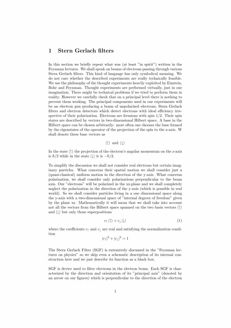
SGF is device used to filter electrons in the electron beam. Each SGF is char-acterized by the direction and orientation of its ”principal axis” (denoted byan arrow on our figures) which is perpendicular to the direction of the electron

1

z

y

x

Figure 1: Stern Gerlach filter

beam going through. The default axial orientation of the SGF is with its arrowpointing vertically upwards.

The function of the SGF in its default position is simple. The electron in thestate |↑〉 passes through the filter without any change of state, electron in thestate |↓〉 is absorbed in the filter and so does not appear on the output side odthe SGF.

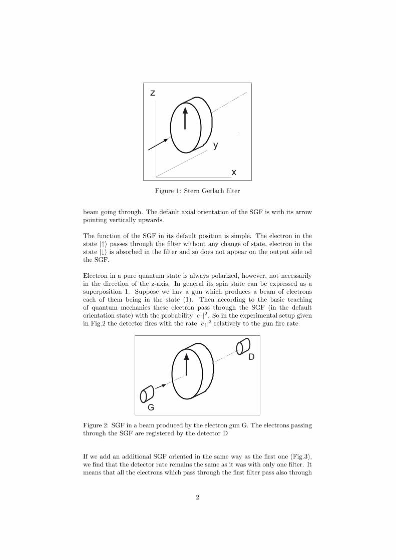
Electron in a pure quantum state is always polarized, however, not necessarilyin the direction of the z-axis. In general its spin state can be expressed as asuperposition 1. Suppose we hav a gun which produces a beam of electronseach of them being in the state (1). Then according to the basic teachingof quantum mechanics these electron pass through the SGF (in the defaultorientation state) with the probability |c↑|2. So in the experimental setup givenin Fig.2 the detector fires with the rate |c↑|2 relatively to the gun fire rate.

D

G

Figure 2: SGF in a beam produced by the electron gun G. The electrons passingthrough the SGF are registered by the detector D

If we add an additional SGF oriented in the same way as the first one (Fig.3),we find that the detector rate remains the same as it was with only one filter. Itmeans that all the electrons which pass through the first filter pass also through

2

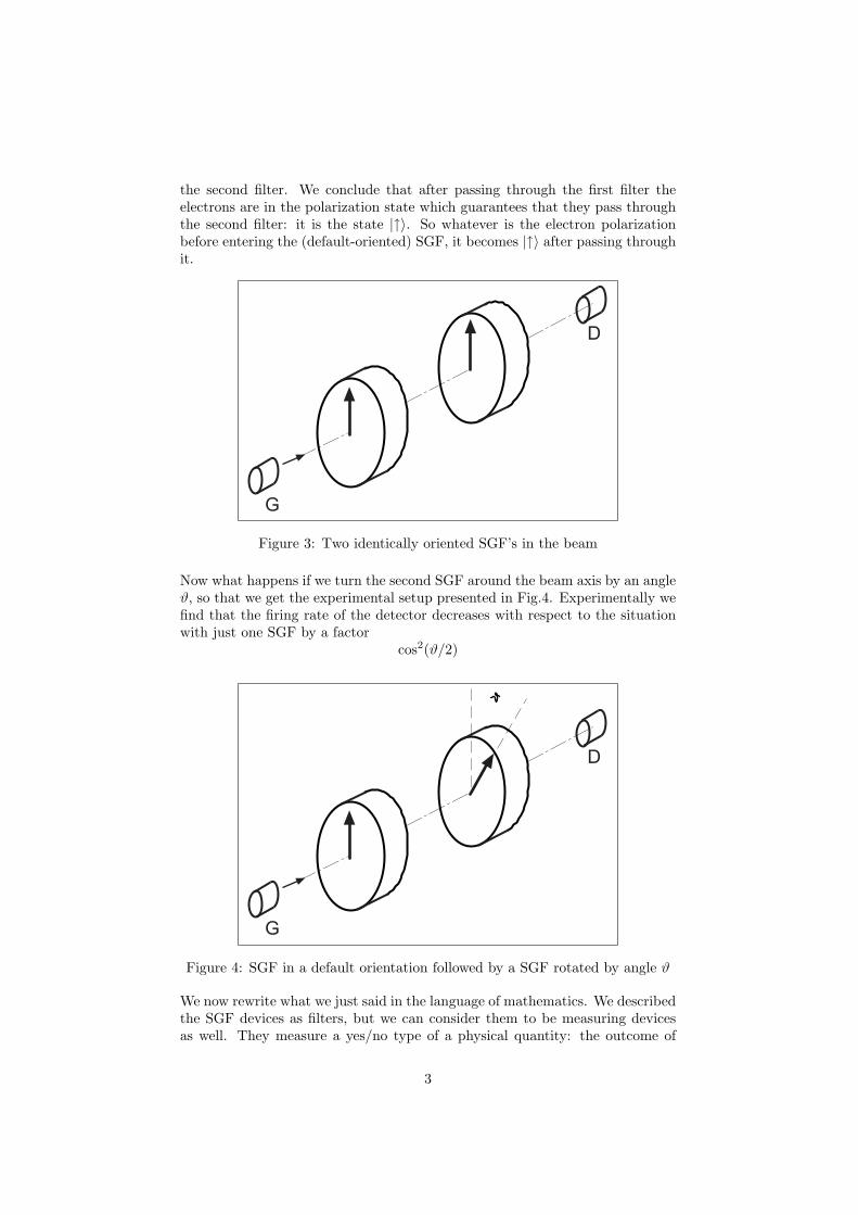
the second filter. We conclude that after passing through the first filter theelectrons are in the polarization state which guarantees that they pass throughthe second filter: it is the state |↑〉. So whatever is the electron polarizationbefore entering the (default-oriented) SGF, it becomes |↑〉 after passing throughit.

D

G

Figure 3: Two identically oriented SGF’s in the beam

Now what happens if we turn the second SGF around the beam axis by an angleϑ, so that we get the experimental setup presented in Fig.4. Experimentally wefind that the firing rate of the detector decreases with respect to the situationwith just one SGF by a factor

cos2(ϑ/2)

D

G

Figure 4: SGF in a default orientation followed by a SGF rotated by angle ϑ

We now rewrite what we just said in the language of mathematics. We describedthe SGF devices as filters, but we can consider them to be measuring devicesas well. They measure a yes/no type of a physical quantity: the outcome of

3

the measurement by the SGF is either 1 or 0 according to whether the electronpasses through the filter or not. It is easy to see that the hermitean operatorcorresponding to the SGF in its default orientation is

P↑ = |↑〉〈↑|

Really, this operator has two eigenstates |↑〉 and |↓〉 corresponding to the eigen-values 1 and 0.

P↑ |↑〉 = |↑〉〈↑|↑〉

P↑ |↓〉 = |↑〉〈↑|↓〉 = 0

Now let us discuss in the same way the SGF rotated axially by the angle ϑ.We shall denote this SGF as SGF(ϑ). Obviously if we take the state |↑〉 androtate it by angle ϑ in the zx-plane we get the state which is guaranteed to passthrough SGF(ϑ). Formally it is the rotation with respect to the beam (y-axis).The corresponding transformation is performed by the unitary operator

exp(−ihϑσy/2)

where σy is the Pauli matrix

σy =(

0 −ii 0

)Using this rotation operator we get for the rotated state

|ϑ〉 = |↑〉 cos(ϑ/2) + |↓〉 sin(ϑ/2) (2)

So the hermitean operator corresponding to SGF(ϑ) is

|ϑ〉 〈ϑ|

On the other hand the state which is guaranteed to be absorbed by the SGF(ϑ)is the state obtained from |↓〉 by rotation by angle ϑ) It is the state

|ϑ⊥〉 = − |↑〉 sin(ϑ/2) + |↓〉 cos(ϑ/2)

This state is, of course, orthogonal to the state |ϑ〉

〈ϑ⊥ | ϑ〉 = 0

Now we can express the state vectors of our original basis in terms of the rotatedvectors. We get

|↑〉 = |ϑ〉 cos(ϑ/2)− |ϑ⊥〉 sin(ϑ/2) (3)

|↓〉 = |ϑ〉 sin(ϑ/2) + |ϑ⊥〉 cos(ϑ/2)

The interpretation of the Eq.3 is the following

If the system is in the state |↑〉 then it is simultaneously with the probabilitycos2(ϑ/2) in the state |ϑ〉 and with the probability sin2(ϑ/2) in the state|ϑ⊥〉.

4

Now we see the mathematical background behind the experimental setup pre-sented in Fig.4. After the SGF(↑) the system is in the state |↑〉 so with theprobability cos2(ϑ/2) it pases through the SGF(ϑ) and with the probabilitysin2(ϑ/2) it is absorbed by it.

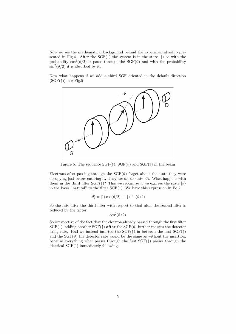
Now what happens if we add a third SGF oriented in the default direction(SGF(↑)), see Fig.5

D

G

Figure 5: The sequence SGF(↑), SGF(ϑ) and SGF(↑) in the beam

Electrons after passing through the SGF(ϑ) forget about the state they wereoccupying just before entering it. They are set to state |ϑ〉. What happens withthem in the third filter SGF(↑)? This we recognize if we express the state |ϑ〉in the basis ”natural” to the filter SGF(↑). We have this expression in Eq.2

|ϑ〉 = |↑〉 cos(ϑ/2) + |↓〉 sin(ϑ/2)

So the rate after the third filter with respect to that after the second filter isreduced by the factor

cos2(ϑ/2)

So irrespective of the fact that the electron already passed through the first filterSGF(↑), adding another SGF(↑) after the SGF(ϑ) further reduces the detectorfiring rate. Had we instead inserted the SGF(↑) in between the first SGF(↑)and the SGF(ϑ) the detector rate would be the same as without the insertion,because everything what passes through the first SGF(↑) passes through theidentical SGF(↑) immediately following.

5

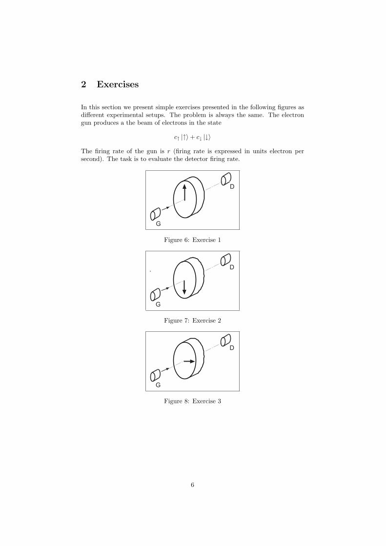
2 Exercises

In this section we present simple exercises presented in the following figures asdifferent experimental setups. The problem is always the same. The electrongun produces a the beam of electrons in the state

c↑ |↑〉+ c↓ |↓〉

The firing rate of the gun is r (firing rate is expressed in units electron persecond). The task is to evaluate the detector firing rate.

D

G

Figure 6: Exercise 1

D

G

Figure 7: Exercise 2

D

G

Figure 8: Exercise 3

6

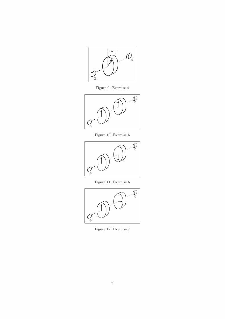
D

G

Figure 9: Exercise 4

D

G

Figure 10: Exercise 5

D

G

Figure 11: Exercise 6

D

G

Figure 12: Exercise 7

7

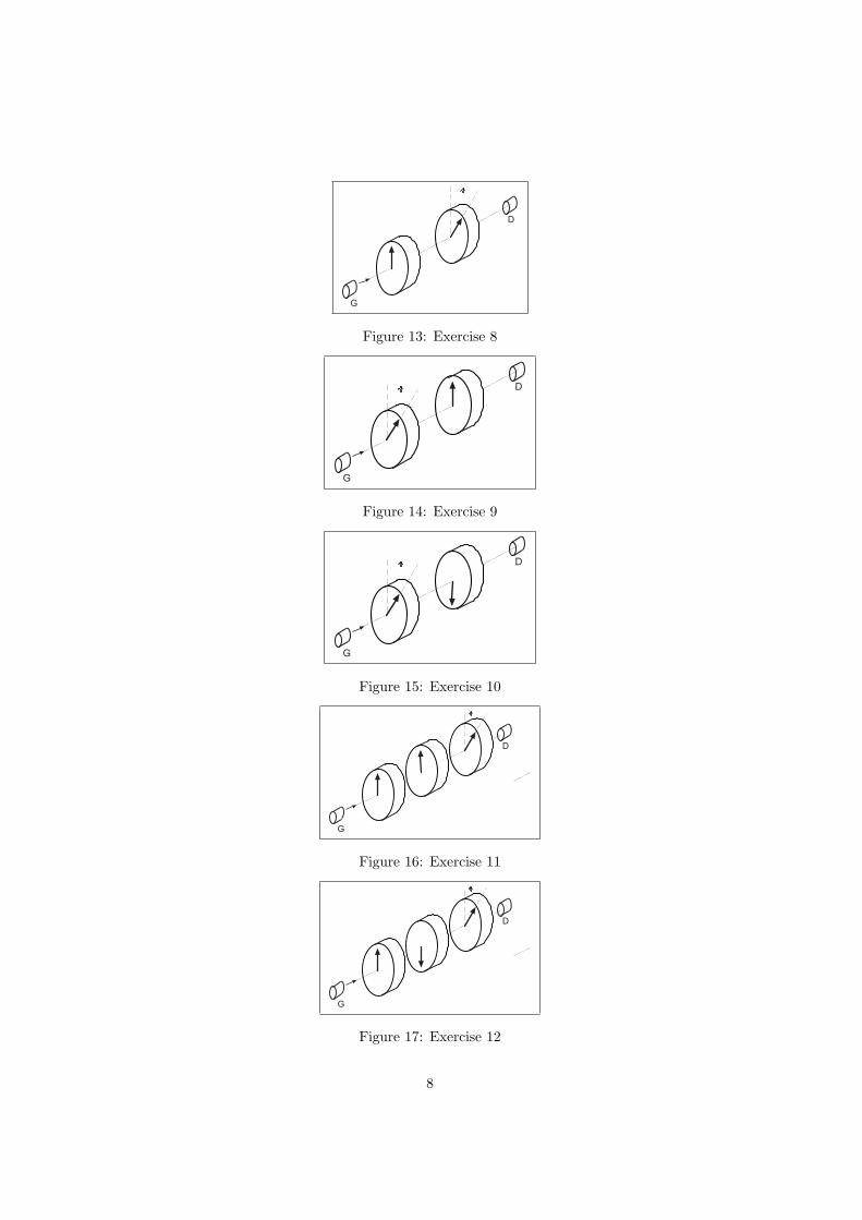
D

G

Figure 13: Exercise 8

D

G

Figure 14: Exercise 9

D

G

Figure 15: Exercise 10

D

G

Figure 16: Exercise 11

D

G

Figure 17: Exercise 12

8

D

G

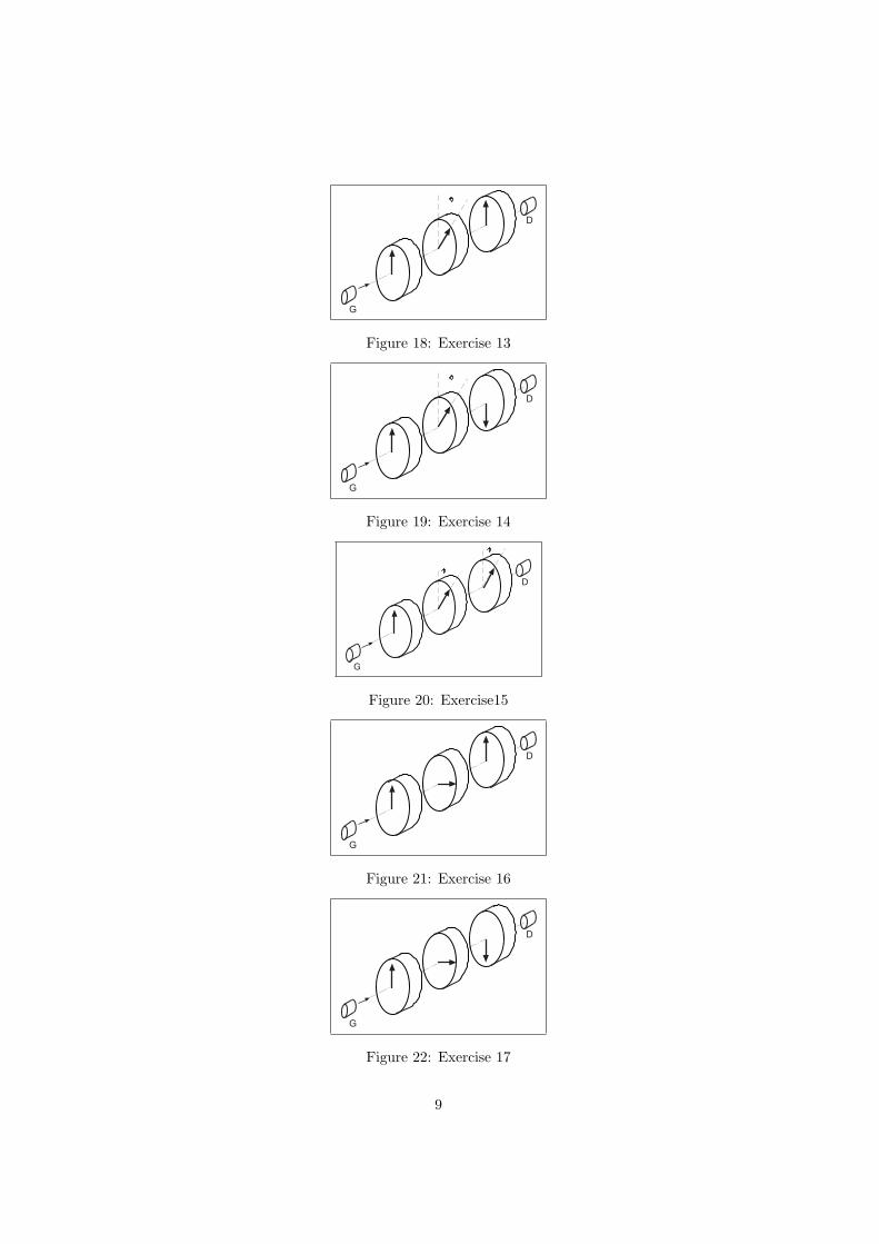
Figure 18: Exercise 13

D

G

Figure 19: Exercise 14

D

G

Figure 20: Exercise15

D

G

Figure 21: Exercise 16

D

G

Figure 22: Exercise 17

9

D

G

Figure 23: Exercise 18

D

G

Figure 24: Exercise 19

10

3 Logic of quantum states

The discussion of the first section and the following exercises have provided uswith the ”experimental evidence” for the following statement.

If an electron passes through two SGF devices which are axially rotated toeach other the electron forgets the state it had coming out from the firstSGF and its state after the second SGF is completely determined by thatsecond SGF. Each SGF imprints on the electron a state given by that SGFonly, not depending on the previous history of the electron states.

The boxed statement is really strange, if we reexpress it in the language of SGF’sas measuring devices.

Let us consider the SGF(↑). We can imagine a small display on the SGF whichshows ”1” when an electron entered the device and went through it and itshows ”0” when the electron entered but did not go through (it was absorbed,diverted to some other direction, whatever). The electron entered the SGF insome (perhaps even unknown) in-state and after the interaction with the SGFan out-state was imprinted on it. If the reading of the display was ”1” theimprinted out-state is ket ↑, if the reading was ”0” did not get out of the SGF.

So the reading of the measuring apparatus is directly related to the out-state ofthe electron, not that much to the in-state. In fact the only thing we can inferabout the in-state using the information from the display is that the in-statewas not orthogonal to the imprinted out-state. Saying it differently: the instate was such that there was a non-zero probability that the outcome of themeasurement would be that one which was really observed. Nothing more.

This is completely contradictory to the creed of the experimental gurus fromthe pre-quantum era. They believed that the purpose of a measurement is todetermine the in-state and that the ideal apparatus shows the relevant informa-tion from which the in-state can be inferred without substantially influencingthat in-state. In other words they believed that one can determine the in-stateby the measurement and the out-state after the measurement will be identicalto the in-state.

All the experimental evidence of the quantum mechanics shows that kind ofbelief was wrong. The only exception is the situation when we use the twoidentical measuring devices one after the other within an infinitesimal timeinterval. The the reading of the second apparatus would be the same as that ofthe first one and the out-state after the second device would be the same as thein-state, because that in-state relevant for the second apparatus is the out-statecoming from the first measuring device.

It is difficult to digest this fact. We know that Einstein felt very uneasy aboutit and continued inventing thought experiments trying to beat the teachingof Bohr about mutual incompatibility of measuring both the position and the

11

momentum of a particle. (The correspondence between Einstein and Bohr onthat matter is well known and reading it is a quite fascinating experience.) Itseems that Einstein finally accepted the possibility of the mutually incompatiblemeasurements.

Mathematically the incompatibility of two measurements is expressed via non-commutability of the operators corresponding to the measuring devices.

In the Hilbert space of the electron polarizations any two different non-trivialhermitean operators do not commute. In the language of SGF’s it means thatany two filters axially rotated with respect to each other are mutually incom-patible. The corresponding hermitean operators do not commute. For example

|↑〉 〈↑| does not commute with |ϑ〉 〈ϑ| for ϑ 6= 0

In more complicated systems there may exist mutually commuting systems ofindependent hermitean operators. The corresponding measurements are thencompatible what means that in a sequence of measurements like

A followed by B followed again by A

the system ”remembers” the value of the physical quantity A found in the firstmeasurement and the renewed measurement of A following the intermediatemeasurement of B reveals exactly the same value of A as found by the firstmeasurement if the operators corresponding to A and B commute.

So let us return to our simple space of the electron polarizations and discuss theconsequences of the mutual incompatibility of measurements.

Suppose we have an electron coming out of the electron gun in an unknownstate. We have several SGF’s on stock with different axial orientation and wewant to perform some measurement on the incoming state. The main point isthat we have just one trial. Whatever measuring device we use, the incomingstate is lost forever. If we subsequently take another apparatus we perform themeasurement on a different state, not on the original one.

So before making the measurement we have to make a decision which apparatusto take (which orientation of the SGF). The decision is final: once the mea-surement is performed it cannot be undone to reconsider the situation or makeanother choice. We make the decision, make the measurement, read the resultand from then on we know the state of the system. We might be curious to knowwhat would have been the result if we had chosen some other apparatus butwe cannot resolve that question. At least this is the teaching of the orthodoxquantum mechanics.

So given the incoming particle we can get the result of the measurement by anysingle apparatus available but not by two (or more) of them: simultaneousvalues of two (non-commuting)physical quantities are inaccessible.

12

This opens the way for situations quite contradictory to ”standard logical think-ing”. Suppose we have an electron in an unknown state we choose to use theSGF(↑) and we find that this particular electron did go through. And afterthat we ask the question: If we had decided to use the SGF(π) apparatus in-stead, would it go through or not? A very strange question indeed, because thetwo devices in question, the SGF(↑) and the SGF(π) are not only incompati-ble (non commuting) they are ”mutually exclusive”: any electron which wentthrough SGF(↑) will not go through the subsequent SGF(π) for sure. And viceversa.

Our intuition then forces us to the conclusion that an electron which can gothrough the SGF(↑) cannot go through the SGF(π). This conclusion is notlogically justified: mutual exclusivity of subsequent events does not inhibit theirconcurrent possibility.

The concurrent possibility of mutually exclusive states in quantum mechanics ismathematically expressed by the superposition principle: the existence of twoarbitrary states implies the existence of any state which can be expressed as asuperposition of the corresponding vectors in the Hilbert space. The fact thatthe two considered states are mutually exclusive means that their correspondingvectors are orthogonal. There is nothing strange in making superpositions ofmutually orthogonal vectors. Just the opposite is true, we prefer to use orthog-onal bases for making superpositions.

In this way an arbitrary polarization state |ϑ〉 can be expressed as a superposi-tion of the mutually exclusive states |↑〉 and |π〉.(See Eq.2)

|ϑ〉 = |↑〉 cos(ϑ/2) + |π〉 sin(ϑ/2)

What we see here is in fact typical for quantum state: two mutually exclusivestates |↑〉 and |π〉 as ”concurrent possibilities” within a single quantum state|ϑ〉.

To illustrate more clearly what is strange on quantum states let us discuss asimple classical system a single die. The die has six faces labelled as 1, 2, 3,4, 5, 6. We shall consider some measuring devices reading the state of the die.To have some resemblance with our quantum filters we shall consider now onlydevices which show on their displays 1 or 0 and the interpretation depends onthe type of the device which can be easily inferred from its name. So for examplethe measuring device labelled as

GREATER-THEN-4

shows on its display 1 if the number read on the die is 5 or 6 and it shows 0 inother cases.

Let us forget for the moment that we know that it is the die what we observe

13

with our devices and that we even do not understand the meaning of the Englishwords on the labels of the measuring devices. We just throw the die then mea-sure it with different devices (we are in the classical world, so the measurementdoes not change the state!) prepare another state by throwing the die, measureit again and so on. Gaining more and more experimental data we find certainrules to hold. Something like the following.

GREATER-THEN-4 is not mutually exclusive with LESS-THEN-6 becausethere are states for which both the devices show 1 on their displays.

GREATER-THEN-4 excludes EQUAL-TO-3

ODD-NUMBER is mutually exclusive with EQUAL-TO-FOUR

After all we recognize that the devices labelled by ”EQUAL-TO” form a specialrecognizable subset from all the devices we have. These devices are special since

• They form a complete set what means that for any state at least one ofthem shows 1 on its display.

• They are all mutually exclusive, what means that never more then one ofthem shows 1.

• They are irreducible what means that for any two states such that forboth of them the same ”EQUAL-TO” device show 1 then the readings onall the other devices for these two states are equal.

It follows from these properties that any other measuring device can be con-structed from the elementary ”EQUAL-TO” by the logical XOR-gates. Forexample

LESS-THEN-3 = EQUAL-TO-1 XOR EQUAL-TO-2

We can use OR-gates instead of exclusive XOR-gates, sice the elementary de-vices are mutually exclusive anyhow.

The states corresponding to the irreducible complete mutually exclusive mea-surements are in the same way irreducible, complete and mutually exclusive.These elementary states can be represented by the sets

{1}, {2}, {3}, {4}, {5}, {6}

The elementary states are ”microstates”: the term borrowed from the statis-tical physics denoting the state which is completely determined (no missinginformation or ”zero” entropy). All the other classical states are ”macrostates”,incompletely determined states (non-zero entropy) which can be constructedfrom the elementary state by the set operation ∪. For example the state

{1} ∪ {2} ∪ {3}

14

is the state recognized by the measuring device LESS-THEN-4 . In the classicalworld the operator OR is therefore represented by the set operator ∪.

So in classical world we can also have ”concurrent mutually exclusive possi-bilities” when allowing for macrostates. These are mixtures of the elementarystates. Different instances of the same macrostate can be treated (for a par-ticular purpose) as equivalent, they are not ”ontologically” equal. Refining themeasurement proces I can always distinguish between different instances of thesame macrostate until I arrive to the level of elementary states which are notfurther reducible. Therefore I assume that all the instances of the elementarystate are for all practical purposes equivalent. I can treat them as if they werethe same. So, referring to the Occam’s razor, they are the same.

In the classical world the ”concurrent mutually exclusive possibilities” impliesreducibility. In the quantum world, at least in the orthodox quantum world, wehave quite a different situation. As we have seen concurrent mutually exclusivepossibilities are realized not only as mixtures 1 but as pure states as well, thepure states: the superpositions. The superposition is a trick how to get bothirreducibility and ”concurrent mutually exclusive possibilities”.

If the ”concurrent mutually exclusive possibilities” are labelled by the logicalsymbol ”XOR” than this quantum mechanical XOR cannot be mathematicallymodelled as unions of disjoined sets because disjoined sets imply reducibility(each element of the union can be uniquely identified as belonging to exactlyone of the disjoined subsets). So if we believe to the irreducibility of the purequantum state, we must have different model of logic: the quantum mechanicalXOR is modelled as linear superposition of mutually orthogonal vectors.

So the question is why we believe to the irreducibility of the states such as

|ϑ〉 = |↑〉 cos(ϑ/2) + |π〉 sin(ϑ/2)

To investigate this problem we have to make experiments with instances of thestate |ϑ〉. Let us imagine that we are the pioneers who are discovering thequantum world and are playing the same game with the quantum devices aswas described above about the pioneers in the classical world investigating thegame of dice.

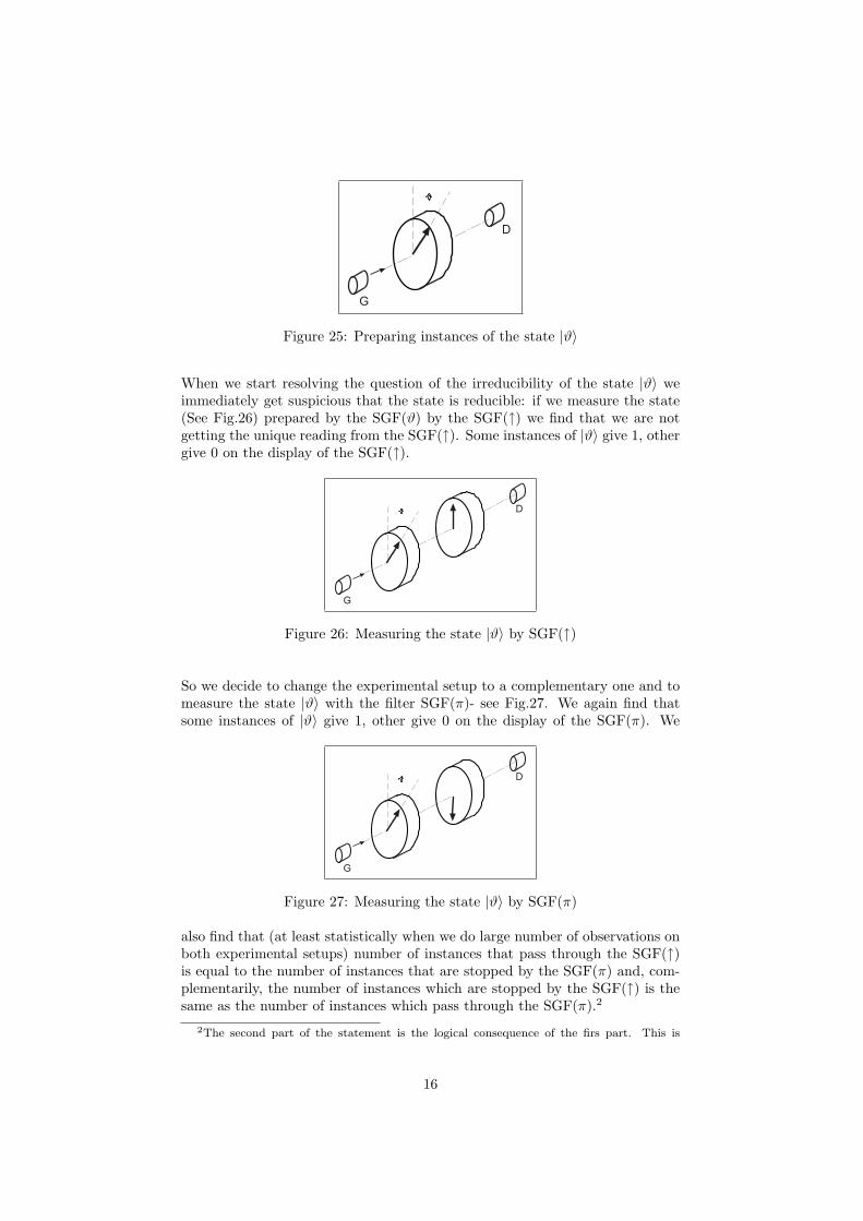
So the state |ϑ〉 is the polarization state of any electron which passed through theSGF(ϑ). So if the electron is found behind the filter (See Fig.25) it is assumedto be in the state |ϑ〉, more exactly it is assumed to be in some instance ofthe state |ϑ〉. We try to be unbiased and allow for possible reducibility of thestate prepared by the filter SGF(ϑ) and therefore we allow for a possibility ofunequivalent instances of the state |ϑ〉.

1We have not discussed mixtures of pure quantum states in this text. The mixture statescan be created in meny different ways. The most transparent one is for example to producean electron beam by randomly switching between two electron guns. If the guns produceelectrons in different states the beam is the statistical mixture of electrons: some of themare the instances of the quantum state produced by the first gun, the other are instances ofthe state produced by the second gun. The resulting state is a ”macrostate”. Without goingto details we just say that such a macrostate is mathematically described byt the densitymatrix.

15

D

G

Figure 25: Preparing instances of the state |ϑ〉

When we start resolving the question of the irreducibility of the state |ϑ〉 weimmediately get suspicious that the state is reducible: if we measure the state(See Fig.26) prepared by the SGF(ϑ) by the SGF(↑) we find that we are notgetting the unique reading from the SGF(↑). Some instances of |ϑ〉 give 1, othergive 0 on the display of the SGF(↑).

D

G

Figure 26: Measuring the state |ϑ〉 by SGF(↑)

So we decide to change the experimental setup to a complementary one and tomeasure the state |ϑ〉 with the filter SGF(π)- see Fig.27. We again find thatsome instances of |ϑ〉 give 1, other give 0 on the display of the SGF(π). We

D

G

Figure 27: Measuring the state |ϑ〉 by SGF(π)

also find that (at least statistically when we do large number of observations onboth experimental setups) number of instances that pass through the SGF(↑)is equal to the number of instances that are stopped by the SGF(π) and, com-plementarily, the number of instances which are stopped by the SGF(↑) is thesame as the number of instances which pass through the SGF(π).2

2The second part of the statement is the logical consequence of the firs part. This is

16

It seems that we have the classification of the instances of the state |ϑ〉 intotwo distinct classes: those which pass through the SGF(↑) and those whichpass through the SGF(π). However, this is an unjustified conclusion. Fromthe observed numbers we cannot infer that the instances which pass throughthe SGF(↑) are those which are stopped by the SGF(π). Such a hypothesis isconsistent with what was said, but is not necessary.

Here is an example with specific numbers. Suppose we had 200 electrons passedthrough the first SGF(ϑ). 100 of them was subsequently measured by theSGF(↑): 60 passed through and 40 were stopped. The other 100 electronswere measured byt the SGF(π), 40 passed and 60 were stopped. One solu-tion is obviously that we have two classes of states: one (pass, stop) the other(stop, pass) and we had 120 states of the first class and 80 states of the secondclass. Another solution may be that we have four classes (pass,pass),(pass,stop),(stop,pass) and (stop,stop). And we had for example 30 states of the first class,30 states of the second class, 10 states of the third class and 30 states of thefourth class. And it seems we cannot resolve which reduction is the correctone because we would need the result of the simultaneous measurement (on thesame instance of the state) with both the filters, which is not possible.

Experimenting further we find that even if such a reduction was true it cannotbe the full story. Because we find that we can make very similar reduction witha different pair of filters, for example with SGF(π/2) and SGF(3π/2). And weneed even more classes of states.

The orthodox quantum mechanics offers an elegant solution of the problem: allpossible reductions but no elementary states: linear superposition opens the wayfor having all possible reductions simultaneously. The choice of base vectors ina linear space is arbitrary. No decomposition into disjoint sets ever happens, sono elementary states. But no ”classical logic” XOR operation either! Quantummechanical XOR is not the union of disjoint sets, it is a linear superposition. Butthe prediction of the outcome of a particular measurement is non-deterministic,instead of unique predictions quantum mechanics offers probabilities.

4 Hidden parameters

We have just described two possible solutions of the state classification problemin the quantum world. One is the orthodox quantum mechanical descriptionwith essential probabilities. The other option is to have much richer space ofstates: each quantum state is decomposed into disjoint sets of more elementarystates. There are many classification schemes of this type consistent with theresult of measurements, at least of the measurement of the type described inthe exercises in Section 2. Disjoint elementary states allow for classical logicand determinism. Such theories are called theories with hidden parameters. Weshall present one specific example of such a theory further below.

because the readings of the measuring devices are classical states, therefore standard logic isapplicable. The readings 1 and 0 are elementary mutually exclusive complete events.

17

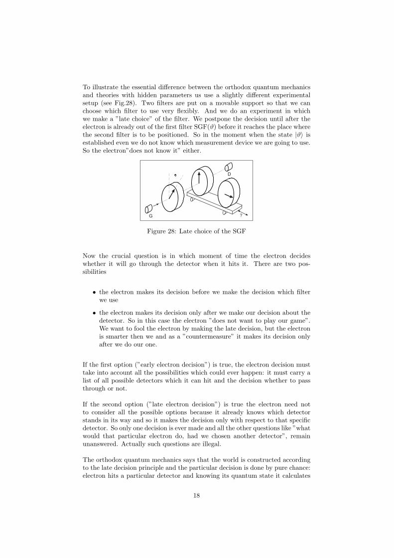
To illustrate the essential difference between the orthodox quantum mechanicsand theories with hidden parameters us use a slightly different experimentalsetup (see Fig.28). Two filters are put on a movable support so that we canchoose which filter to use very flexibly. And we do an experiment in whichwe make a ”late choice” of the filter. We postpone the decision until after theelectron is already out of the first filter SGF(ϑ) before it reaches the place wherethe second filter is to be positioned. So in the moment when the state |ϑ〉 isestablished even we do not know which measurement device we are going to use.So the electron”does not know it” either.

D

G ?

Figure 28: Late choice of the SGF

Now the crucial question is in which moment of time the electron decideswhether it will go through the detector when it hits it. There are two pos-sibilities

• the electron makes its decision before we make the decision which filterwe use

• the electron makes its decision only after we make our decision about thedetector. So in this case the electron ”does not want to play our game”.We want to fool the electron by making the late decision, but the electronis smarter then we and as a ”countermeasure” it makes its decision onlyafter we do our one.

If the first option (”early electron decision”) is true, the electron decision musttake into account all the possibilities which could ever happen: it must carry alist of all possible detectors which it can hit and the decision whether to passthrough or not.

If the second option (”late electron decision”) is true the electron need notto consider all the possible options because it already knows which detectorstands in its way and so it makes the decision only with respect to that specificdetector. So only one decision is ever made and all the other questions like ”whatwould that particular electron do, had we chosen another detector”, remainunanswered. Actually such questions are illegal.

The orthodox quantum mechanics says that the world is constructed accordingto the late decision principle and the particular decision is done by pure chance:electron hits a particular detector and knowing its quantum state it calculates

18

the probability p to pass through it. It then plays the dice: it generates arandom number ξ ∈ (0, 1) and if ξ < p it goes through, else it is stopped.

Let us now describe in somewhat more detail a specific ”early electron decisionmodel”. The essential point is that everything is decided in the moment whenthe electron is leaving the ”state preparing” filter. As we have already agreedthe filter ”imprints” on the leaving electron the out-state. In the early decisionmodel the out-state not only carries the information which particular filter hasprepared the state, but also the information from which one can deterministi-cally deduce whether the electron passes through any thinkable filter which canfollow.

Let us assume that the piece of information in the out-state which codes thestate preparing measurement will be identical to that in the quantum mechan-ics. So if the device was SGF(ϑ), the ”complete” out-state is formed by thecorresponding vector from the standard Hilbert space plus a single real param-eter λ ∈ (0, 1). This parameter codes the ”behind the quantum mechanics”information on the outcome of all the possible future experiments. In our caseof electron polarizations all the measurement are done with the SGF filters.Since no two SGF filters can be applied simultaneously, the set of ”all the pos-sible future experiments” is quite simple: it is the set of SGF filters arbitrarilyaxially rotated. The parameter λ has to code the outcome of measurement byarbitrarily rotated filter SGF(ϕ). Let us take a simple coding:

if λ < cos2(ϑ− ϕ

2) electron passes through, otherwise it is stopped

As an exercise the reader can verify, that if the parameter λ is a random numberdistributed uniformly in the interval (0, 1), the results of all the experiments ofthe type described in the Section 2 are the same as in the orthodox quantummechanics. The parameter λ is called the ”hidden parameter”: we do not haveany theory on its dynamics, we cannot measure it by any available apparatus.It is just an arbitrary mathematical tool which changes the late-decision-typequantum theory into the early-decision-type theory.

Introducing the hidden parameter we were able to decompose the quantum stateinto elementary mutually exclusive states labelled by λ, we have classical ”XOR-composition” of states modelled by set union operator. However, the differencebetween the hidden-parameter theory and our classical example of the states ofthe die is that the decomposition into the elementary disjoint states does nothave the corresponding counterpart in the space of measuring devices. The pointis that we cannot drop the ”typically quantum” feature of changing the stateafter each measurement. The electron in the incoming hidden-parameter-state

(|ϑ〉 , λ)

after passing through the filter SGF(ϕ) will be in the out-state

(|ϕ〉 , λ′)

where the new value of the hidden parameter λ′ is a new random number withno correlation to the old value λ whatsoever. Otherwise the predictions of the

19

new hidden-parameter-theory would be different from those of pure quantummechanics and ruled out by the experiment.

Since we do not have the decomposition of measuring devices into ”elementarymutually disjoint complete system” our theory with the hidden parameters isstill not ”completely classical”. Some questions which are legal in the classicalphysics may be illegal in quantum theory even in the presence of the hiddenparameters, because the measuring devices are still mutually incompatible”. Sothe crucial question

We have chosen to use the filter SGF(ϕ) and the electron passed through.What would be the outcome had we chosen the filter SGF(ϕ′)?

is illegal in the hidden-parameter theory in the same way as it is in the orthodoxquantum mechanics. We cannot attack experimentally such a problem becauseof mutual incompatibility of different SGF’s.

Let us repeat briefly the argumentation leading to such a conclusion

• Different SGF’s are described by non-commuting operators therefore theireigenstates and eigenvalues are mutually incompatible

• By physical construction two different SGF’s cannot be used simultane-ously but only in sequence.

• The state of the electron leaving the filter is changed with respect to whatit was before entering the filter.

• Subsequent measurement is performed on the changed state.

• Therefore it is (experimentally) illegal to speak about simultaneous valuesof mutually incompatible physical quantities.

On the other hand in our particular model of the hidden-parameter theory thequestion is legal an can be answered by the theory. Knowing the parameter λ wecan answer the question what would be the outcome of all thinkable experiments.Unfortunately, the parameter λ is hidden from us. It should be also stressed thatit is possible to formulate theories having more hidden parameters for which theanswers to questions concerning alternative choice of measuring devices would bequite different. However experiments we have discussed so far cannot distinguishbetween various hidden-parameter theories nor between the orthodox quantummechanics and any reasonable hidden parameter theory.

However Einstein, Rosen and Podolski realized that there is a flaw in the aboveargumentation concerning experimental inaccessibility of simultaneous values ofmutually incompatible quantities.

We said already that Einstein was very much willing to have simultaneous val-ues of mutually incompatible quantities in the theory, but by force of the Bohr’s

20

argumentation,he had to retreat from his position and accept mutual incompat-ibility of operators and the change of state by measurement.

The theory with hidden parameters provides the way to have both determin-ism and indeterminism and both simultaneous values of physical quantities andmutual incompatibility of measurements. The prize one has to pay for it is theincompatibility between the ontological status and the gnoseological status ofthe theory: the state of the system cannot be recognized as it really is. Onto-logically the outcome of the measurement is deterministic, gnoseologically thepredictions of the theory are only probabilistic.

Such a status of the theory could be hardly acceptable for Einstein. (Justrecall that it was the very careful analysis of the measurement of time intervalsand clock synchronization which paved the way for abandoning the notion ofabsolute time.)

The message of the EPR paper was that there is a way how to make the simul-taneous values of incompatible quantities experimentally accessible while stillaccepting all the Bohr’s arguments about incompatible measurements.

5 The EPR idea

The primer interest of authors of the EPR paper was the question of simultane-ous measurement of the position and momentum with a precision higher thenthat compatible with the uncertainty principle. We shall rewrite the story fortwo incompatible SGF filters.

EPR realized that there might be a way to experimentally access incompatiblequantities simultaneously. The task is to measure two incompatible quantities3

SGF(ϑ) and SGF(ϕ) on a given (arbitrary but unknown) electron state. TheEPR trick is that we measure one quantity, say SGF(ϑ), on the given electronand the other measurement we perform indirectly. We do not apply the deviceSGF(ϕ) on the given electron, this is not possible without interfering with themeasurement of SGF(ϑ).

Instead we measure some other suitable quantity on some other system andthis other quantity is carefully chosen in such a way that from its value wecan deduce what would be the value found by the measurement of SGF(ϕ)on the given electron had we chosen to measure SGF(ϕ) instead of SGF(ϑ).

It should be stressed that whatever the EPR suggestion is, it cannot work inthe orthodox quantum mechanics: in the late-decision-type theory the questionof simultaneous values of incompatible quantities is strictly illegal. Whatever

3Here we again use the language treating SGF’s as measuring devices: the SGF(ϑ) mea-sures the quantity represented by the operator |ϑ〉 〈ϑ|. Then instead of saying ”the quantitymeasured by the device SGF(ϑ)” we simply say the quantity SGF(ϑ).

21

the EPR procedure is, the result of it cannot and must not be interpreted as thesimultaneous measurement of quantities within the orthodox quantum theory.

The EPR paper wanted to show that in the early-decision-type of theory withhidden parameters theoretically existing simultaneous values can be measured(at least in some cases).

The observation of the EPR is that in some cases we expect strong correlationsbetween different physical quantities. That opens a way how to deduce the valueof some quantity without measuring it directly: we can measure some otherquantity with which it is correlated and from the result of that measurementwe can calculate the value which interests us.

A typical example of strong correlation is represented by any conservation law.For example if we know the total energy of some system which consists of twosubsystems and later on we measure the energy of one of the subsystems, thenwe do not need to measure the energy of the other subsystem. We can calculateits value using the energy-conservation law.

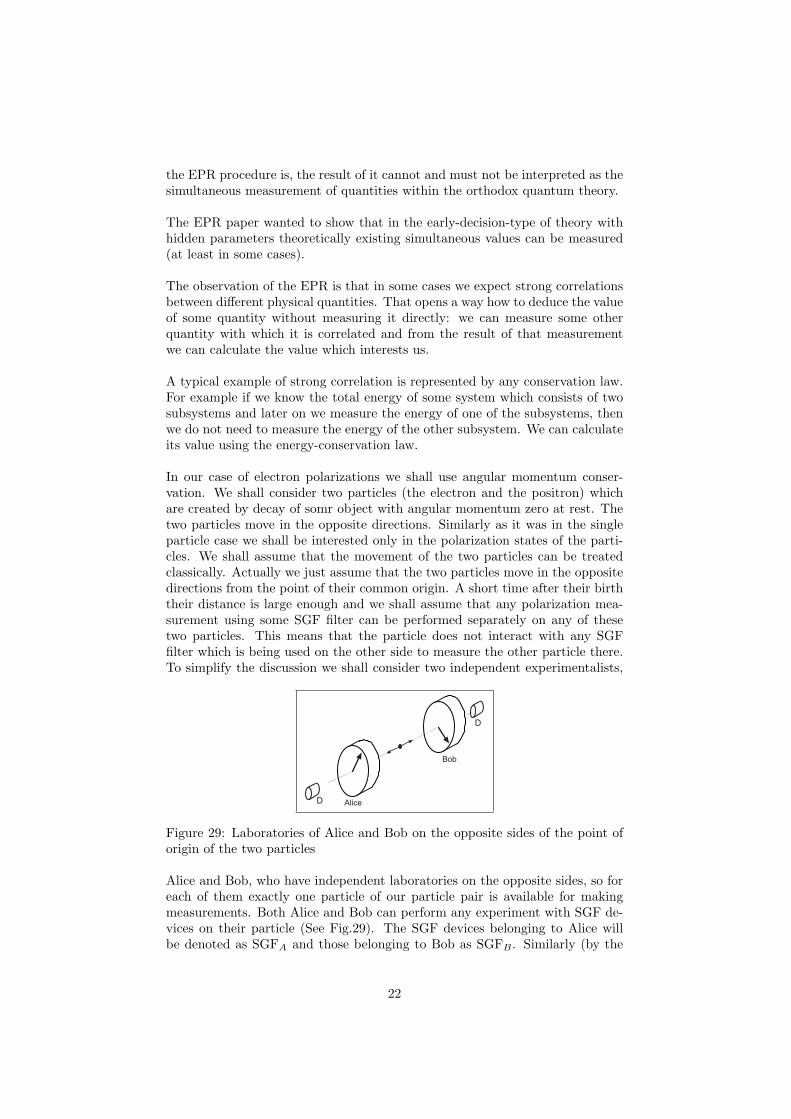
In our case of electron polarizations we shall use angular momentum conser-vation. We shall consider two particles (the electron and the positron) whichare created by decay of somr object with angular momentum zero at rest. Thetwo particles move in the opposite directions. Similarly as it was in the singleparticle case we shall be interested only in the polarization states of the parti-cles. We shall assume that the movement of the two particles can be treatedclassically. Actually we just assume that the two particles move in the oppositedirections from the point of their common origin. A short time after their birththeir distance is large enough and we shall assume that any polarization mea-surement using some SGF filter can be performed separately on any of thesetwo particles. This means that the particle does not interact with any SGFfilter which is being used on the other side to measure the other particle there.To simplify the discussion we shall consider two independent experimentalists,

D

D Alice

Bob

Figure 29: Laboratories of Alice and Bob on the opposite sides of the point oforigin of the two particles

Alice and Bob, who have independent laboratories on the opposite sides, so foreach of them exactly one particle of our particle pair is available for makingmeasurements. Both Alice and Bob can perform any experiment with SGF de-vices on their particle (See Fig.29). The SGF devices belonging to Alice willbe denoted as SGFA and those belonging to Bob as SGFB . Similarly (by the

22

appropriate index) we shall distinguish the single particle states.

6 EPR in orthodox quantum theory

We shall start our discussion within the framework of the orthodox quantummechanics. We shall call the initial polarization two-particle state as the EPRstate. Without going into details4 we just write the EPR state in terms of singleparticle states as

|EPR〉 =1√2|↑A〉 |↓B〉 −

1√2|↓A〉 |↑B〉

In the above equation we have used specific base states |↑〉 and |↓〉. However, the|EPR〉 state is symmetric with respect to axial rotation, and so its expressionusing any other (rotated) base will be the same5, for example

|EPR〉 =1√2|ϑA〉 |ϑ⊥B〉 −

1√2|ϑ⊥A〉 |ϑB〉

To worm up we first do a few easy exercises. First we calculate the probabil-ity pA(↑) that the Alice’s particle passes through SGFA(↑). The appropriateoperator is |↑A〉〈↑A|. We get

p(↑A) = 〈EPR |↑A〉〈↑A| EPR〉 =12

Now calculate the probability that Bob’s particle passes through SGFB(π/3).Theappropriate operator is |(π/3)B〉|(π/3)B〉. Realizing that

〈↑B | (π/3)B〉 = cos(π/6)

〈↓B | (π/3)B〉 = sin(π/6)

We get

p((π/3)B) = 〈EPR | (π/3)B〉 〈(π/3)B | EPR〉 =12(cos2(π/6) + sin2(π/6)

)=

12

In general we get

p(ϑB) =12

4The reader not familiar with rules of angular momentum composition can find the relevantinformation in any textbook on quantum mechanics, where he shall look for the keyword”Clebsh-Gordan coefficients.

5Because of this axial symmetry of the EPR state every result we shall obtain will dependonly on relative angles between the devices in Alice’s laboratory with respect to those in Bob’slaboratory.

23

for arbitrary angle ϑ. And the same is true, of course, for Alice’s measurements.

However, things start to be more interesting when we look for correlations. Forexample let us calculate the joint probability that Alice’s particle passes throughSGFA(↑) and Bob’s particle passes through SGFB(π/3). The appropriate op-erator now is

|↑A〉 |(π/3)B〉〈(π/3)B | 〈↑A|

and we get

p(↑A, (π/3)B) = 〈EPR |↑A〉 |(π/3)B〉 〈(π/3)B | 〈↑A| EPR〉 =12

sin2(π/6) =18

So we see there is a correlation between the outcomes of the measurements onthe Alice’s and Bob’s sides since

18

= p(↑A, (π/3)B) 6= p(↑A)p((π/3)B) =14

Let us now calculate the joint probability that Alice’s particle passes throughSGFA(↑) and Bob’s particle does not pass through SGFB(π/3). The appropriateoperator now is (

|↑A〉 〈↑A|)(

1− |(π/3)B〉 〈(π/3)B |)

and we get

p(↑A, NOT (π/3)B) = 〈EPR|(|↑A〉 〈↑A|

)(1− |(π/3)B〉 〈(π/3)B |

)|EPR〉 =

=12− 1

2sin2(π/6) =

38

Similarly we can calculate the remaining two possibilities of the joint probabilityand we get

p(NOT ↑A, (π/3)B) =38

p(NOT ↑A, NOT (π/3)B) =18

Total correlation between Alice’s and Bob’s measurements using SGFA(↑) andSGFB(π). We get

p(↑A, πB) = 1/2

p(↑A, NOTπB) = 0

p(NOT ↑A, πB) = 0

p(NOT ↑A, NOTπB) = 1/2

To fact of the total correlation is better seen from the conditional probabilities.For example

p(↑A, πB) = p(πB | ↑A)p(↑A)

24

Since p(↑A) = 1/2 and p(↑A, πB) = 1/2, we get

p(πB | ↑A) = 1

where p(πB | ↑A) is the conditional probability that Bob’s particle passes throughthe SGFB(π) if we know that Alice’s particle passed through the SGFA(↑).

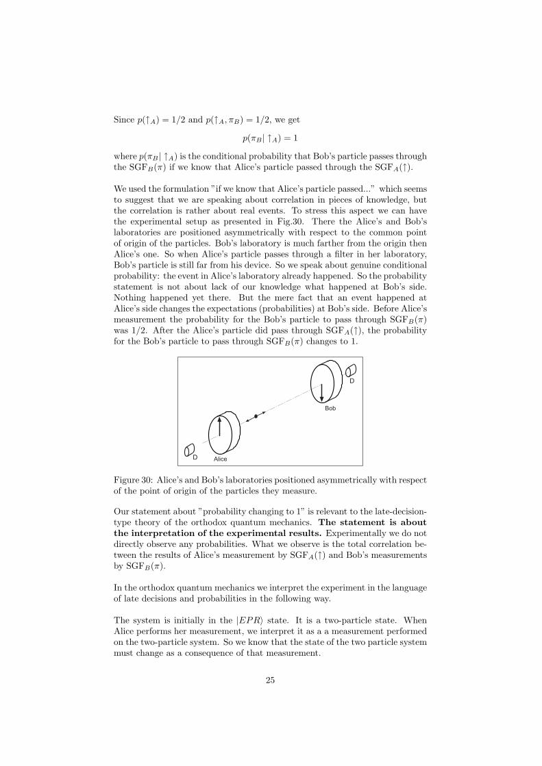
We used the formulation ”if we know that Alice’s particle passed...” which seemsto suggest that we are speaking about correlation in pieces of knowledge, butthe correlation is rather about real events. To stress this aspect we can havethe experimental setup as presented in Fig.30. There the Alice’s and Bob’slaboratories are positioned asymmetrically with respect to the common pointof origin of the particles. Bob’s laboratory is much farther from the origin thenAlice’s one. So when Alice’s particle passes through a filter in her laboratory,Bob’s particle is still far from his device. So we speak about genuine conditionalprobability: the event in Alice’s laboratory already happened. So the probabilitystatement is not about lack of our knowledge what happened at Bob’s side.Nothing happened yet there. But the mere fact that an event happened atAlice’s side changes the expectations (probabilities) at Bob’s side. Before Alice’smeasurement the probability for the Bob’s particle to pass through SGFB(π)was 1/2. After the Alice’s particle did pass through SGFA(↑), the probabilityfor the Bob’s particle to pass through SGFB(π) changes to 1.

D

D Alice

Bob

Figure 30: Alice’s and Bob’s laboratories positioned asymmetrically with respectof the point of origin of the particles they measure.

Our statement about ”probability changing to 1” is relevant to the late-decision-type theory of the orthodox quantum mechanics. The statement is aboutthe interpretation of the experimental results. Experimentally we do notdirectly observe any probabilities. What we observe is the total correlation be-tween the results of Alice’s measurement by SGFA(↑) and Bob’s measurementsby SGFB(π).

In the orthodox quantum mechanics we interpret the experiment in the languageof late decisions and probabilities in the following way.

The system is initially in the |EPR〉 state. It is a two-particle state. WhenAlice performs her measurement, we interpret it as a a measurement performedon the two-particle system. So we know that the state of the two particle systemmust change as a consequence of that measurement.

25

The only measuring devices we consider in these notes are the SGF filters. Theoperators corresponding to such devices are projectors. In that case the rule howto write down the out-state (the state of the system after the measurement) fromthe in-state (the state of the system before the measurement) is quite simple.It is described in the following box.

• We begin with properly normalized |in-state〉

• The operator corresponding to SGF(ϑ) is the projection operator

P = |ϑ〉 〈ϑ|

• We apply the projection operator to the in-state and get an auxiliaryvector

|aux〉 = P |in-state〉

• We get the out-state of the particle which passed through the filter fromthe auxiliary vector by normalizing it to 1:

|out-state〉 =1√

〈aux | aux〉|aux〉

Applying this algorithm to the situation after the Alice found that her particledid pass through the filter SGFA(↑)

|aux〉 = |↑A〉 〈↑A| EPR〉 =

= |↑A〉 〈↑A|(

1√2|↑A〉 |↓B〉 −

1√2|↓A〉 |↑B〉

)=

=1√2|↑A〉 |↓B〉

|out-state〉 = |↑A〉 |↓B〉

The |out-state〉 is the two-particle state! It is the state of the system just afterAlice’s experiment and before the Bob’s experiment. So it is the in-state fromthe point of view of Bob. By inspection it is now clear why the Bob’s particlepasses through SGFB(π) with certainty.

Similar absolute correlation we get for any pair of SGF’s relatively rotated toeach other by the angle π.

As an exercise the reader can prove that there is a total autocorrelation betweenAlice and Bob if they use a pair of equally oriented SGF’s.

7 EPR and hidden parameters

The theory with hidden parameters is the early-decision theory. It means thatthe outcome of any future experiment must be decided in the moment of ”birth”

26

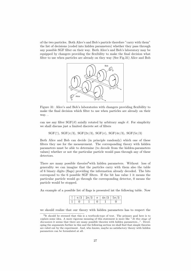
of the two particles. Both Alice’s and Bob’s particle therefore ”carry with them”the list of decisions (coded into hidden parameters) whether they pass throughany possible SGF filter on their way. Both Alice’s and Bob’s laboratory may beequipped by changers providing the flexibility to make the final decision whatfilter to use when particles are already on they way (See Fig.31) Alice and Bob

D

D

Alice

Bob

Figure 31: Alice’s and Bob’s laboratories with changers providing flexibility tomake the final decision which filter to use when particles are already on theirway. .

can use any filter SGF(ϑ) axially rotated by arbitrary angle ϑ. For simplicitywe shall discuss just a limited discrete set of filters

SGF(↑), SGF(π/3), SGF(2π/3), SGF(π), SGF(4π/3), SGF(5π/3)

Both Alice and Bob can decide (in principle randomly) which one of thesefilters they use for the measurement. The corresponding theory with hiddenparameters must be able to determine (to decode from the hidden-parametersvalues) whether or not the particular particle would pass through any of thesedetectors.

There are many possible theories6with hidden parameters. Without loss ofgenerality we can imagine that the particles carry with them also the tableof 6 binary digits (flags) providing the information already decoded. The bitscorrespond to the 6 possible SGF filters. If the bit has value 1 it means theparticular particle would go through the corresponding detector, 0 means theparticle would be stopped.

An example of a possible list of flags is presented int the following table. Now

↑ π/3 2π/3 π 4π/3 5π/31 0 1 0 1 0

we should realize that our theory with hidden parameters has to respect the6It should be stressed that this is a textbook-type of text. The primary goal here is to

explain some idea. A more rigorous meaning of this statement is more like ”At this stage ofdiscussion it seems that there are many possible theories with hidden parameters...”. Devel-oping the arguments further in this and the following section we shall find that simple theoriesare ruled out by the experiment. And, who knows, maybe no satisfactory theory with hiddenparameters can be formulated at all.

27

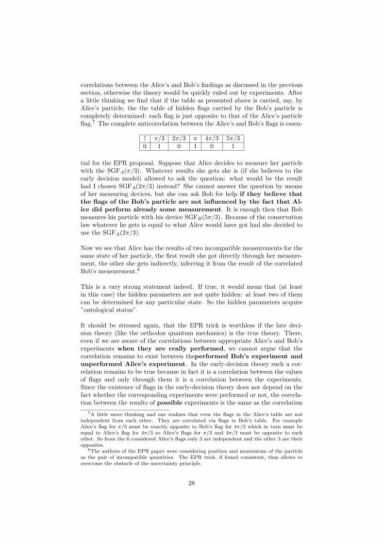
correlations between the Alice’s and Bob’s findings as discussed in the previoussection, otherwise the theory would be quickly ruled out by experiments. Aftera little thinking we find that if the table as presented above is carried, say, byAlice’s particle, the the table of hidden flags carried by the Bob’s particle iscompletely determined: each flag is just opposite to that of the Alice’s particleflag.7 The complete anticorrelation between the Alice’s and Bob’s flags is essen-

↑ π/3 2π/3 π 4π/3 5π/30 1 0 1 0 1

tial for the EPR proposal. Suppose that Alice decides to measure her particlewith the SGFA(π/3). Whatever results she gets she is (if she believes to theearly decision model) allowed to ask the question: what would be the resulthad I chosen SGFA(2π/3) instead? She cannot answer the question by meansof her measuring devices, but she can ask Bob for help if they believe thatthe flags of the Bob’s particle are not influenced by the fact that Al-ice did perform already some measurement. It is enough then that Bobmeasures his particle with his device SGFB(5π/3). Because of the conservationlaw whatever he gets is equal to what Alice would have got had she decided touse the SGFA(2π/3).

Now we see that Alice has the results of two incompatible measurements for thesame state of her particle, the first result she got directly through her measure-ment, the other she gets indirectly, inferring it from the result of the correlatedBob’s measurement.8

This is a vary strong statement indeed. If true, it would mean that (at leastin this case) the hidden parameters are not quite hidden: at least two of themcan be determined for any particular state. So the hidden parameters acquire”ontological status”.

It should be stressed again, that the EPR trick is worthless if the late deci-sion theory (like the orthodox quantum mechanics) is the true theory. There,even if we are aware of the correlations between appropriate Alice’s and Bob’sexperiments when they are really performed, we cannot argue that thecorrelation remains to exist between theperformed Bob’s experiment andunperformed Alice’s experiment. In the early-decision theory such a cor-relation remains to be true because in fact it is a correlation between the valuesof flags and only through them it is a correlation between the experiments.Since the existence of flags in the early-decision theory does not depend on thefact whether the corresponding experiments were performed or not, the correla-tion between the results of possible experiments is the same as the correlation

7A little more thinking and one realizes that even the flags in the Alice’s table are notindependent from each other. They are correlated via flags in Bob’s table. For exampleAlice’s flag for π/3 must be exactly opposite to Bob’s flag for 4π/3 which in turn must beequal to Alice’s flag for 4π/3 so Alice’s flags for π/3 and 4π/3 must be opposite to eachother. So from the 6 considered Alice’s flags only 3 are independent and the other 3 are theiropposites.

8The authors of the EPR paper were considering position and momentum of the particleas the pair of incompatible quantities. The EPR trick, if found consistent, thus allows toovercome the obstacle of the uncertainty principle.

28

between the experiments really performed.

8 Bell inequalities

The theory with hidden parameters seems to be very attractive. The question isto what extend it is compatible with the results of existing experiments. Sinceno experiment so far performed was found to be inconsistent with the predictionsof the orthodox quantum mechanics, the crucial question is to what extent thepredictions of the hidden-parameter theory can be made close to the predictionsof the orthodox quantum mechanics.

Let us first consider the single particle experiments. The question is whetherwe can assign probabilities to all the possible flag tables in such a way thatall the single particle experiments give the same results as in the orthodoxquantum theory. Since we know that for the |EPR〉 state the probability ofa single particle to pass through any filter is 1/2, it is enough to set the flagsjust randomly to reproduce all the single particle experiments.9 So there existsa hidden-parameter theory which gives for the single particle experiments thesame results as the orthodox quantum mechanics. Therefore it is not possibleto distinguish between the late-decision and early-decision theories by singleparticle experiments with the |EPR〉 state.

So we have to turn to correlation experiments performed simultaneously inAlice’s and Bob’s laboratories and try to design a strategy which would helpto distinguish between the early-decision and late-decision theories. So thequestion is whether there exists a hidden parameter theory the results of whichare undistinguishable from the orthodox quantum theory for both single particleand correlation type of experiments.

The answer is due to J.Bell and is negative. It can be proved that no hiddenparameter theory10 can reproduce the results of quantum mechanics for allcorrelation experiments. The proof is surprisingly simple. Let us consider theexperimental situation as presented in Fig.31. We shall consider 3 experimentalsetups as presented in the following table The experimental procedure will be

Experiment Alice Bob1 SGFA(↑) SGFB(5π/3)2 SGFA(2π/3) SGFB(π/3)3 SGFA(4π/3) SGFB(π)

the following. Particle pairs are sequentially produced in the point of origin. Werandomly change the experimental setup choosing randomly between setups ”1”,”2”, and ”3”. Then the cycle is repeated indefinitely. For each pair Alice andBob write down their observation, that is they write down ”1” if they observed

9Of course, theory with randomly assigned flags would be immediately ruled out by thecorrelation experiments.

10More exactly no local hidden parameter theory, see the discussion later.

29

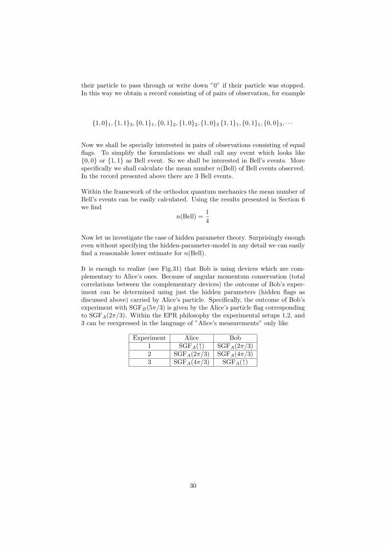
their particle to pass through or write down ”0” if their particle was stopped.In this way we obtain a record consisting of of pairs of observation, for example

{1, 0}1, {1, 1}3, {0, 1}1, {0, 1}2, {1, 0}2, {1, 0}3 {1, 1}1, {0, 1}1, {0, 0}3, · · ·

Now we shall be specially interested in pairs of observations consisting of equalflags. To simplify the formulations we shall call any event which looks like{0, 0} or {1, 1} as Bell event. So we shall be interested in Bell’s events. Morespecifically we shall calculate the mean number n(Bell) of Bell events observed.In the record presented above there are 3 Bell events.

Within the framework of the orthodox quantum mechanics the mean number ofBell’s events can be easily calculated. Using the results presented in Section 6we find

n(Bell) =14

Now let us investigate the case of hidden parameter theory. Surprisingly enougheven without specifying the hidden-parameter-model in any detail we can easilyfind a reasonable lower estimate for n(Bell).

It is enough to realize (see Fig.31) that Bob is using devices which are com-plementary to Alice’s ones. Because of angular momentum conservation (totalcorrelations between the complementary devices) the outcome of Bob’s exper-iment can be determined using just the hidden parameters (hidden flags asdiscussed above) carried by Alice’s particle. Specifically, the outcome of Bob’sexperiment with SGFB(5π/3) is given by the Alice’s particle flag correspondingto SGFA(2π/3). Within the EPR philosophy the experimental setups 1,2, and3 can be reexpressed in the language of ”Alice’s measurements” only like

Experiment Alice Bob1 SGFA(↑) SGFA(2π/3)2 SGFA(2π/3) SGFA(4π/3)3 SGFA(4π/3) SGFA(↑)

30

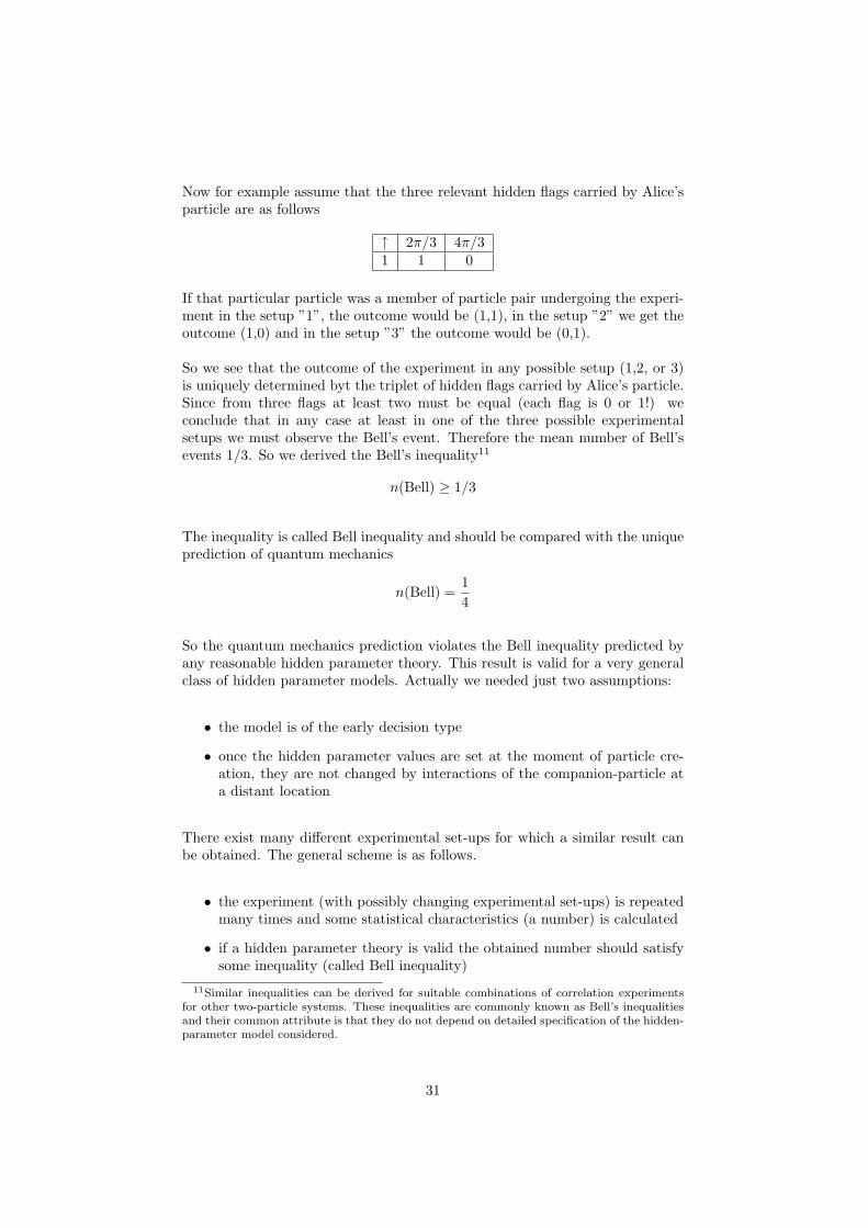
Now for example assume that the three relevant hidden flags carried by Alice’sparticle are as follows

↑ 2π/3 4π/31 1 0

If that particular particle was a member of particle pair undergoing the experi-ment in the setup ”1”, the outcome would be (1,1), in the setup ”2” we get theoutcome (1,0) and in the setup ”3” the outcome would be (0,1).

So we see that the outcome of the experiment in any possible setup (1,2, or 3)is uniquely determined byt the triplet of hidden flags carried by Alice’s particle.Since from three flags at least two must be equal (each flag is 0 or 1!) weconclude that in any case at least in one of the three possible experimentalsetups we must observe the Bell’s event. Therefore the mean number of Bell’sevents 1/3. So we derived the Bell’s inequality11

n(Bell) ≥ 1/3

The inequality is called Bell inequality and should be compared with the uniqueprediction of quantum mechanics

n(Bell) =14

So the quantum mechanics prediction violates the Bell inequality predicted byany reasonable hidden parameter theory. This result is valid for a very generalclass of hidden parameter models. Actually we needed just two assumptions:

• the model is of the early decision type

• once the hidden parameter values are set at the moment of particle cre-ation, they are not changed by interactions of the companion-particle ata distant location

There exist many different experimental set-ups for which a similar result canbe obtained. The general scheme is as follows.

• the experiment (with possibly changing experimental set-ups) is repeatedmany times and some statistical characteristics (a number) is calculated

• if a hidden parameter theory is valid the obtained number should satisfysome inequality (called Bell inequality)

11Similar inequalities can be derived for suitable combinations of correlation experimentsfor other two-particle systems. These inequalities are commonly known as Bell’s inequalitiesand their common attribute is that they do not depend on detailed specification of the hidden-parameter model considered.

31

• If quantum mechanics is valid, than the Bell inequality should be violatedby the number obtained

Of the order of ten experiments of the kind just described were performed andthe majority of them claims finding violation of the relevant Bell inequality.However, the problem is not considered as settled. Many objections were for-mulated by critics suggesting possible flaws in the performed experiments. Thedetails of the discussions are beyond the scope of this notes.

32