1

2

3

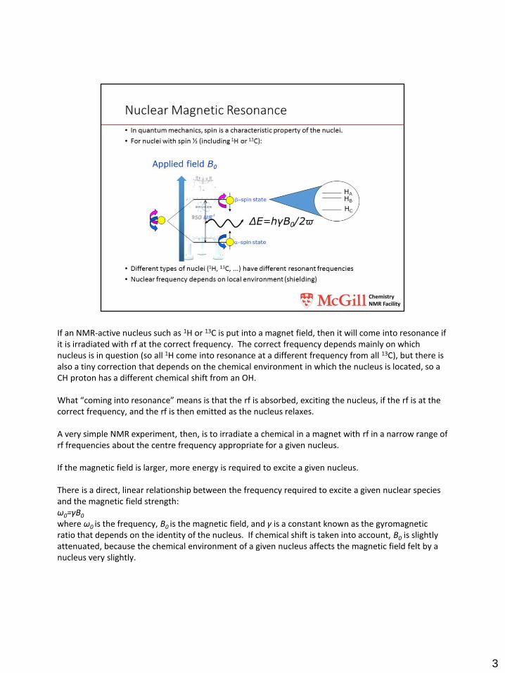
If an NMR-active nucleus such as 1H or 13C is put into a magnet field, then it will come into resonance if it is irradiated with rf at the correct frequency. The correct frequency depends mainly on which nucleus is in question (so all 1H come into resonance at a different frequency from all 13C), but there is also a tiny correction that depends on the chemical environment in which the nucleus is located, so a CH proton has a different chemical shift from an OH.

What “coming into resonance” means is that the rf is absorbed, exciting the nucleus, if the rf is at the correct frequency, and the rf is then emitted as the nucleus relaxes.

A very simple NMR experiment, then, is to irradiate a chemical in a magnet with rf in a narrow range of rf frequencies about the centre frequency appropriate for a given nucleus.

If the magnetic field is larger, more energy is required to excite a given nucleus.

There is a direct, linear relationship between the frequency required to excite a given nuclear species and the magnetic field strength:ω0=γB0

where ω0 is the frequency, B0 is the magnetic field, and γ is a constant known as the gyromagnetic ratio that depends on the identity of the nucleus. If chemical shift is taken into account, B0 is slightly attenuated, because the chemical environment of a given nucleus affects the magnetic field felt by a nucleus very slightly.

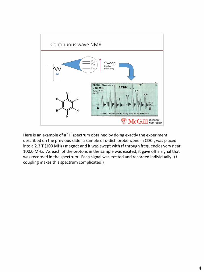
Here is an example of a 1H spectrum obtained by doing exactly the experiment described on the previous slide: a sample of o-dichlorobenzene in CDCl3 was placed into a 2.3 T (100 MHz) magnet and it was swept with rf through frequencies very near 100.0 MHz. As each of the protons in the sample was excited, it gave off a signal that was recorded in the spectrum. Each signal was excited and recorded individually. (J coupling makes this spectrum complicated.)

4

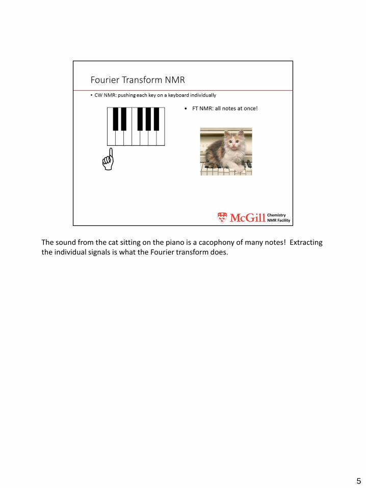
The sound from the cat sitting on the piano is a cacophony of many notes! Extracting the individual signals is what the Fourier transform does.

5

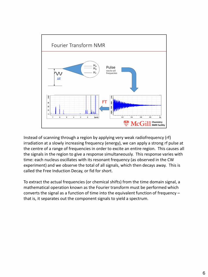
Instead of scanning through a region by applying very weak radiofrequency (rf) irradiation at a slowly increasing frequency (energy), we can apply a strong rf pulse at the centre of a range of frequencies in order to excite an entire region. This causes all the signals in the region to give a response simultaneously. This response varies with time: each nucleus oscillates with its resonant frequency (as observed in the CW experiment) and we observe the total of all signals, which then decays away. This is called the Free Induction Decay, or fid for short.

To extract the actual frequencies (or chemical shifts) from the time domain signal, a mathematical operation known as the Fourier transform must be performed which converts the signal as a function of time into the equivalent function of frequency –that is, it separates out the component signals to yield a spectrum.

6

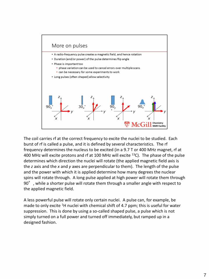
The coil carries rf at the correct frequency to excite the nuclei to be studied. Each burst of rf is called a pulse, and it is defined by several characteristics. The rf frequency determines the nucleus to be excited (in a 9.7 T or 400 MHz magnet, rf at 400 MHz will excite protons and rf at 100 MHz will excite 13C). The phase of the pulse determines which direction the nuclei will rotate (the applied magnetic field axis is the z axis and the x and y axes are perpendicular to them). The length of the pulse and the power with which it is applied determine how many degrees the nuclear spins will rotate through. A long pulse applied at high power will rotate them through 90°, while a shorter pulse will rotate them through a smaller angle with respect to the applied magnetic field.

A less powerful pulse will rotate only certain nuclei. A pulse can, for example, be made to only excite 1H nuclei with chemical shift of 4.7 ppm; this is useful for water suppression. This is done by using a so-called shaped pulse, a pulse which is not simply turned on a full power and turned off immediately, but ramped up in a designed fashion.

7

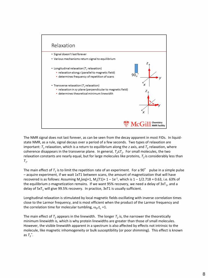
The NMR signal does not last forever, as can be seen from the decay apparent in most FIDs. In liquid-state NMR, as a rule, signal decays over a period of a few seconds. Two types of relaxation are important: T1 relaxation, which is a return to equilibrium along the z axis, and T2 relaxation, where coherence disappears in the transverse plane. In general, T2≤T1. For small molecules, the two relaxation constants are nearly equal, but for large molecules like proteins, T2 is considerably less than T1.

The main effect of T1 is to limit the repetition rate of an experiment. For a 90° pulse in a simple pulse – acquire experiment, if we wait 1xT1 between scans, the amount of magnetization that will have recovered is as follows: Assuming Mz(eq)=1, Mz(T1)= 1 – 1e-1, which is 1 – 1/2.718 = 0.63, i.e. 63% of the equilibrium z-magnetization remains. If we want 95% recovery, we need a delay of 3xT1, and a delay of 5xT1 will give 99.5% recovery. In practice, 3xT1 is usually sufficient.

Longitudinal relaxation is stimulated by local magnetic fields oscillating with inverse correlation times close to the Larmor frequency, and is most efficient when the product of the Larmor frequency and the correlation time for molecular tumbling, w0*tc =1.

The main effect of T2 appears in the linewidth. The longer T2 is, the narrower the theoretically minimum linewidth is, which is why protein linewidths are greater than those of small molecules. However, the visible linewidth apparent in a spectrum is also affected by effects not intrinsic to the molecule, like magnetic inhomogeneity or bulk susceptibility (or poor shimming). This effect is known as T2

*.

8

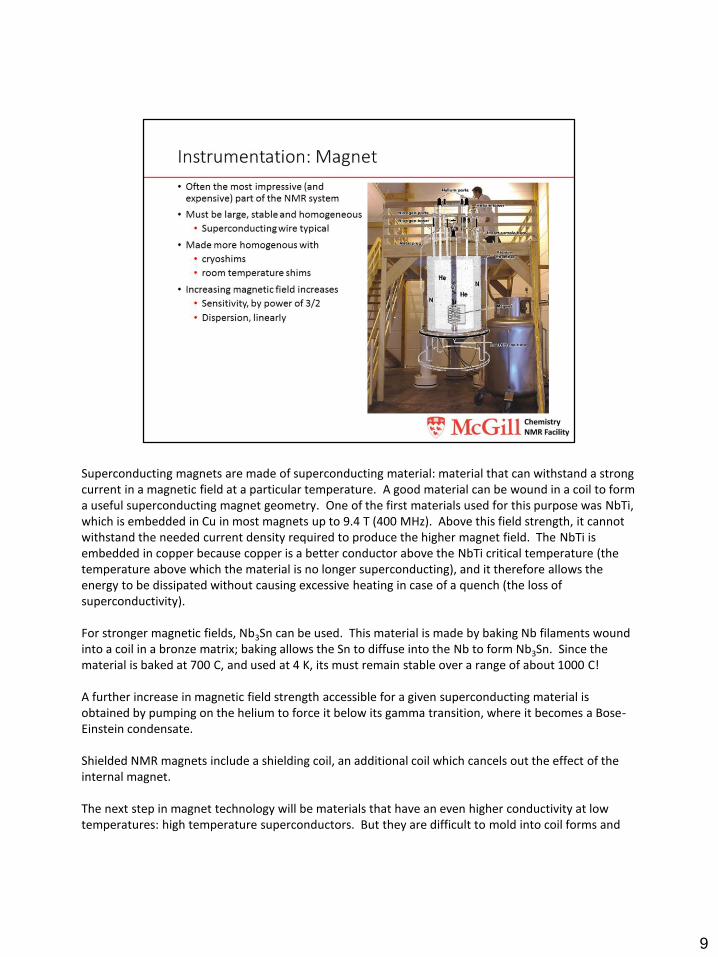
Superconducting magnets are made of superconducting material: material that can withstand a strong current in a magnetic field at a particular temperature. A good material can be wound in a coil to form a useful superconducting magnet geometry. One of the first materials used for this purpose was NbTi, which is embedded in Cu in most magnets up to 9.4 T (400 MHz). Above this field strength, it cannot withstand the needed current density required to produce the higher magnet field. The NbTi is embedded in copper because copper is a better conductor above the NbTi critical temperature (the temperature above which the material is no longer superconducting), and it therefore allows the energy to be dissipated without causing excessive heating in case of a quench (the loss of superconductivity).

For stronger magnetic fields, Nb3Sn can be used. This material is made by baking Nb filaments wound into a coil in a bronze matrix; baking allows the Sn to diffuse into the Nb to form Nb3Sn. Since the material is baked at 700 C, and used at 4 K, its must remain stable over a range of about 1000 C!

A further increase in magnetic field strength accessible for a given superconducting material is obtained by pumping on the helium to force it below its gamma transition, where it becomes a Bose-Einstein condensate.

Shielded NMR magnets include a shielding coil, an additional coil which cancels out the effect of the internal magnet.

The next step in magnet technology will be materials that have an even higher conductivity at low temperatures: high temperature superconductors. But they are difficult to mold into coil forms and

9

much work is going into making them useful.

9

Magnetic field is measured in Tesla (T) or Gauss (G) (1 T = 104 G)But in NMR, the magnetic field strength is usually referred to by the 1H frequency at the given field

Every NMR-active nucleus is excited at a particular frequency in the magnetic fieldthe frequency is measured in Megahertz (MHz)the frequency a nucleus is excited at is directly proportional to the magnetic field

Chemical shifts are very small fractions of the main excitation frequencychemical shifts are measured in ppm, where

1 ppm = [(nucleus excitation frequency in MHz) / 106] Hzchemical shifts in ppm are the same at all frequencies

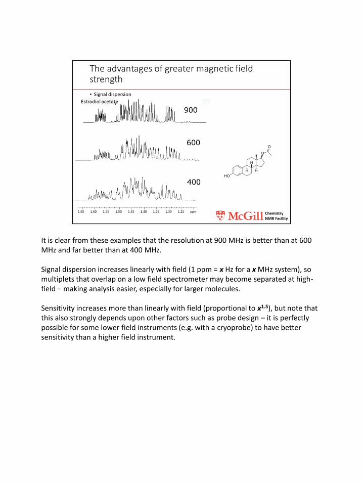
It is clear from these examples that the resolution at 900 MHz is better than at 600 MHz and far better than at 400 MHz.

Signal dispersion increases linearly with field (1 ppm = x Hz for a x MHz system), so multiplets that overlap on a low field spectrometer may become separated at high-field – making analysis easier, especially for larger molecules.

Sensitivity increases more than linearly with field (proportional to x1.5), but note that this also strongly depends upon other factors such as probe design – it is perfectly possible for some lower field instruments (e.g. with a cryoprobe) to have better sensitivity than a higher field instrument.

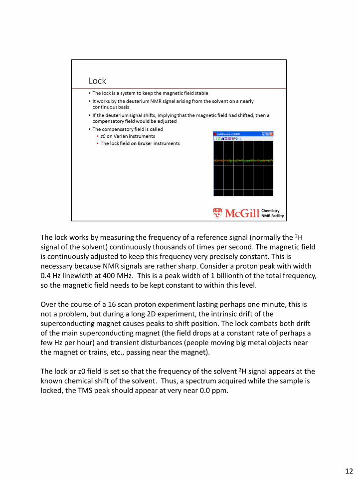
The lock works by measuring the frequency of a reference signal (normally the 2H signal of the solvent) continuously thousands of times per second. The magnetic field is continuously adjusted to keep this frequency very precisely constant. This is necessary because NMR signals are rather sharp. Consider a proton peak with width 0.4 Hz linewidth at 400 MHz. This is a peak width of 1 billionth of the total frequency, so the magnetic field needs to be kept constant to within this level.

Over the course of a 16 scan proton experiment lasting perhaps one minute, this is not a problem, but during a long 2D experiment, the intrinsic drift of the superconducting magnet causes peaks to shift position. The lock combats both drift of the main superconducting magnet (the field drops at a constant rate of perhaps a few Hz per hour) and transient disturbances (people moving big metal objects near the magnet or trains, etc., passing near the magnet).

The lock or z0 field is set so that the frequency of the solvent 2H signal appears at the known chemical shift of the solvent. Thus, a spectrum acquired while the sample is locked, the TMS peak should appear at very near 0.0 ppm.

12

The main magnetic field generated by the superconducting magnet is not quite constant – imperfections in joints etc. introduce a small residual resistance. Typically this leads to a change in proton resonance frequency of ~ a few Hz/hr or less. This is probably insignificant for a 16 scan proton experiment taking only one minute, but would not be tolerable in long experiments taking hours or days. The lock controls an auxiliary (room temperature) field coil, which compensates for changes in the main field. The lock works on very short timescales, and can also correct for transient disturbances (changes of local magnetic field due to movement of metal objects etc.).

14

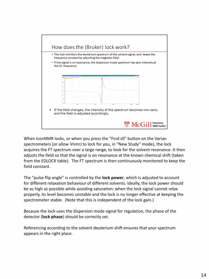
When IconNMR locks, or when you press the “Find z0” button on the Varian spectrometers (or allow VnmrJ to lock for you, in “New Study” mode), the lock acquires the FT spectrum over a large range, to look for the solvent resonance. It then adjusts the field so that the signal is on resonance at the known chemical shift (taken from the EDLOCK table). The FT spectrum is then continuously monitored to keep the field constant.

The “pulse flip angle” is controlled by the lock power, which is adjusted to account for different relaxation behaviour of different solvents. Ideally, the lock power should be as high as possible while avoiding saturation: when the lock signal cannot relax properly, its level becomes unstable and the lock is no longer effective at keeping the spectrometer stable. (Note that this is independent of the lock gain.)

Because the lock uses the dispersion mode signal for regulation, the phase of the detector (lock phase) should be correctly set.

Referencing according to the solvent deuterium shift ensures that your spectrum appears in the right place.

15

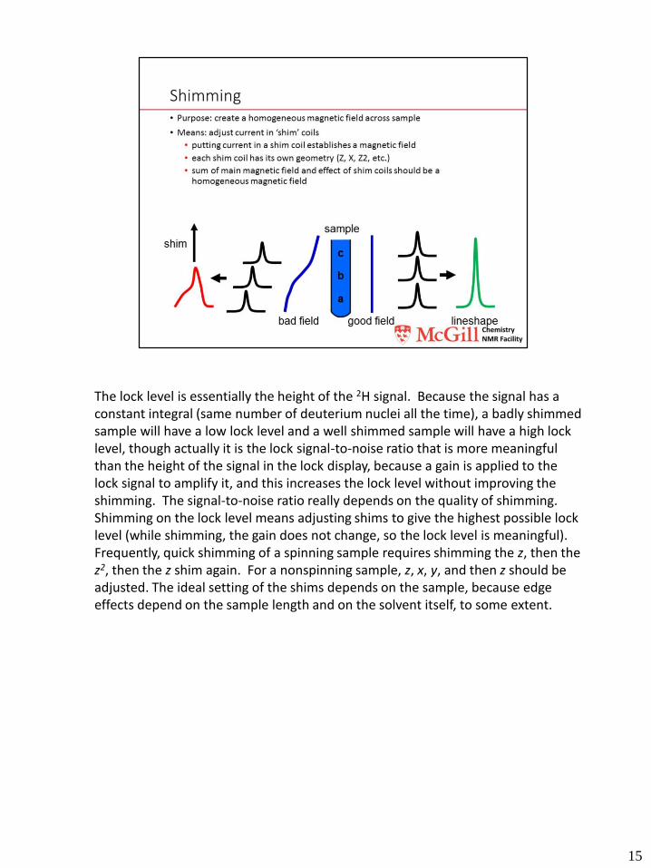
The lock level is essentially the height of the 2H signal. Because the signal has a constant integral (same number of deuterium nuclei all the time), a badly shimmed sample will have a low lock level and a well shimmed sample will have a high lock level, though actually it is the lock signal-to-noise ratio that is more meaningful than the height of the signal in the lock display, because a gain is applied to the lock signal to amplify it, and this increases the lock level without improving the shimming. The signal-to-noise ratio really depends on the quality of shimming.Shimming on the lock level means adjusting shims to give the highest possible lock level (while shimming, the gain does not change, so the lock level is meaningful). Frequently, quick shimming of a spinning sample requires shimming the z, then the z2, then the z shim again. For a nonspinning sample, z, x, y, and then z should be adjusted. The ideal setting of the shims depends on the sample, because edge effects depend on the sample length and on the solvent itself, to some extent.

16

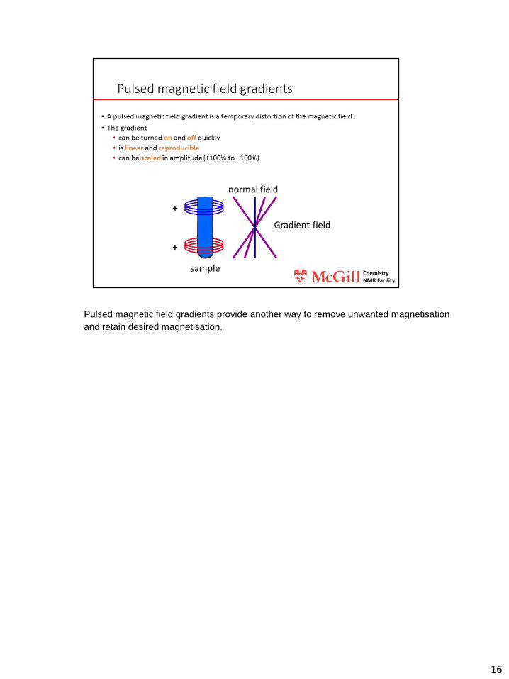
Pulsed magnetic field gradients provide another way to remove unwanted magnetisation

and retain desired magnetisation.

17

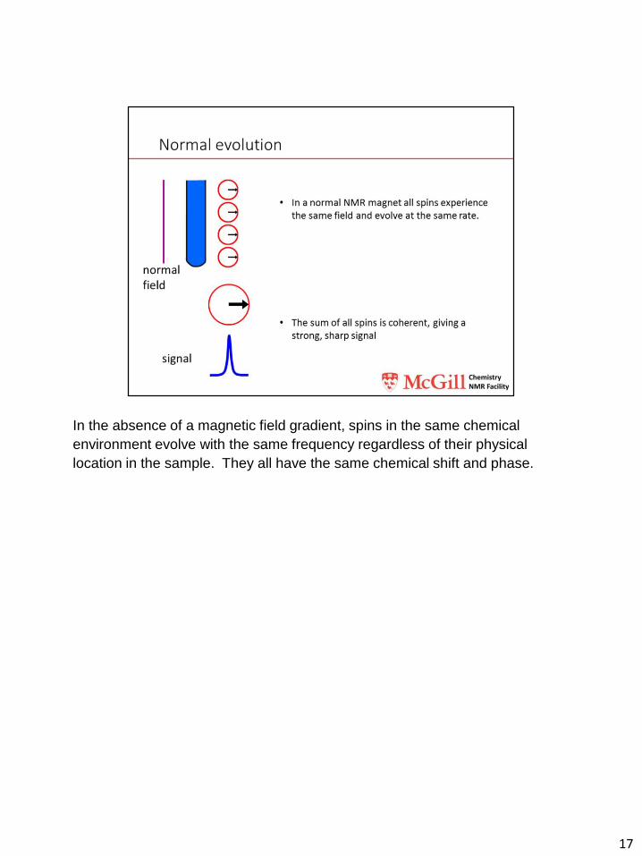
In the absence of a magnetic field gradient, spins in the same chemical

environment evolve with the same frequency regardless of their physical

location in the sample. They all have the same chemical shift and phase.

18

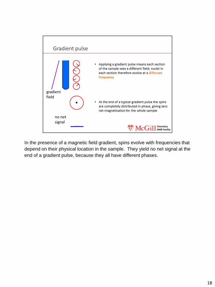
In the presence of a magnetic field gradient, spins evolve with frequencies that

depend on their physical location in the sample. They yield no net signal at the

end of a gradient pulse, because they all have different phases.

19

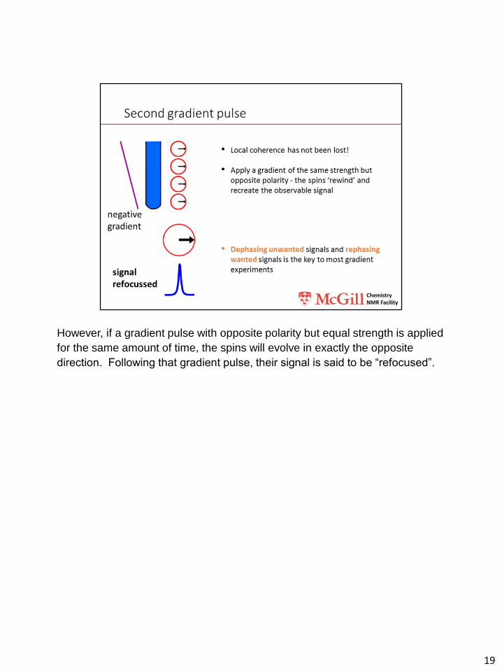
However, if a gradient pulse with opposite polarity but equal strength is applied

for the same amount of time, the spins will evolve in exactly the opposite

direction. Following that gradient pulse, their signal is said to be “refocused”.

20

In both cases, gradient shimming is used to map regions of inhomogeneitiesaround the sample, and decide how best to correct them.

21

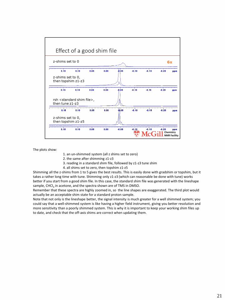
The plots show: 1. an un-shimmed system (all z shims set to zero) 2. the same after shimming z1-z33. reading in a standard shim file, followed by z1-z3 tune shim4. all shims set to zero, then topshim z1-z5

Shimming all the z-shims from 1 to 5 gives the best results. This is easily done with gradshim or topshim, but it takes a rather long time with tune. Shimming only z1-z3 (which can reasonable be done with tune) works better if you start from a good shim file. In this case, the standard shim file was generated with the lineshapesample, CHCl3 in acetone, and the spectra shown are of TMS in DMSO.Remember that these spectra are highly zoomed in, so the line shapes are exaggerated. The third plot would actually be an acceptable shim state for a standard proton sample.Note that not only is the lineshape better, the signal intensity is much greater for a well shimmed system; you could say that a well-shimmed system is like having a higher field instrument, giving you better resolution and more sensitivity than a poorly shimmed system. This is why it is important to keep your working shim files up to date, and check that the off-axis shims are correct when updating them.

22

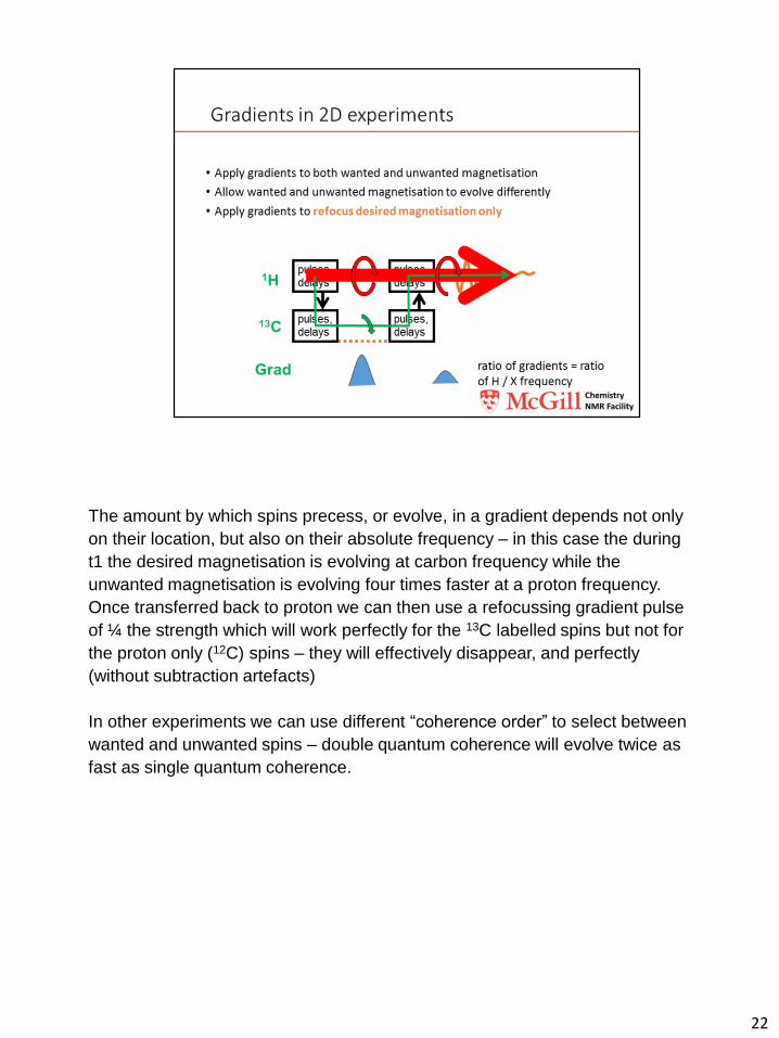
The amount by which spins precess, or evolve, in a gradient depends not only

on their location, but also on their absolute frequency – in this case the during

t1 the desired magnetisation is evolving at carbon frequency while the

unwanted magnetisation is evolving four times faster at a proton frequency.

Once transferred back to proton we can then use a refocussing gradient pulse

of ¼ the strength which will work perfectly for the 13C labelled spins but not for

the proton only (12C) spins – they will effectively disappear, and perfectly

(without subtraction artefacts)

In other experiments we can use different “coherence order” to select between

wanted and unwanted spins – double quantum coherence will evolve twice as

fast as single quantum coherence.

23

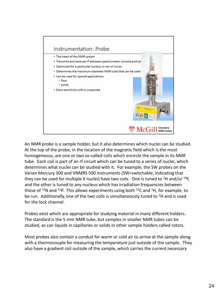
An NMR probe is a sample holder, but it also determines which nuclei can be studied. At the top of the probe, in the location of the magnetic field which is the most homogeneous, are one or two so-called coils which encircle the sample in its NMR tube. Each coil is part of an rf circuit which can be tuned to a series of nuclei, which determines what nuclei can be studied with it. For example, the SW probes on the Varian Mercury 300 and VNMRS 500 instruments (SW=switchable, indicating that they can be used for multiple X nuclei) have two coils. One is tuned to 1H and/or 19F, and the other is tuned to any nucleus which has irradiation frequencies between those of 15N and 31P. This allows experiments using both 13C and 1H, for example, to be run. Additionally, one of the two coils is simultaneously tuned to 2H and is used for the lock channel.

Probes exist which are appropriate for studying material in many different holders. The standard is the 5 mm NMR tube, but samples in smaller NMR tubes can be studied, as can liquids in capillaries or solids in other sample holders called rotors.

Most probes also contain a conduit for warm or cold air to arrive at the sample along with a thermocouple for measuring the temperature just outside of the sample. They also have a gradient coil outside of the sample, which carries the current necessary

24

for inducing a linearly varying magnetic field along the depth of the sample.

24

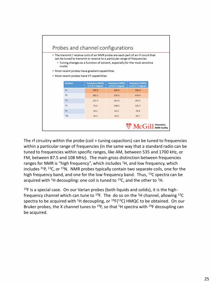
The rf circuitry within the probe (coil + tuning capacitors) can be tuned to frequencies within a particular range of frequencies (in the same way that a standard radio can be tuned to frequencies within specific ranges, like AM, between 535 and 1700 kHz, or FM, between 87.5 and 108 MHz). The main gross distinction between frequencies ranges for NMR is “high frequency”, which includes 1H, and low frequency, which includes 31P, 13C, or 15N. NMR probes typically contain two separate coils, one for the high frequency band, and one for the low frequency band. Thus, 13C spectra can be acquired with 1H decoupling: one coil is tuned to 13C, and the other to 1H.

19F is a special case. On our Varian probes (both liquids and solids), it is the high-frequency channel which can tune to 19F. The do so on the 1H channel, allowing 13C spectra to be acquired with 1H decoupling, or 19F{13C} HMQC to be obtained. On our Bruker probes, the X channel tunes to 19F, so that 1H spectra with 19F decoupling can be acquired.

25

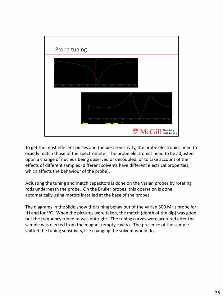
To get the most efficient pulses and the best sensitivity, the probe electronics need to exactly match those of the spectrometer. The probe electronics need to be adjusted upon a change of nucleus being observed or decoupled, or to take account of the effects of different samples (different solvents have different electrical properties, which affects the behaviour of the probe).

Adjusting the tuning and match capacitors is done on the Varian probes by rotating rods underneath the probe. On the Bruker probes, this operation is done automatically using motors installed at the base of the probes.

The diagrams in the slide show the tuning behaviour of the Varian 500 MHz probe for 1H and for 13C. When the pictures were taken, the match (depth of the dip) was good, but the frequency tuned to was not right. The tuning curves were acquired after the sample was ejected from the magnet (empty cavity). The presence of the sample shifted the tuning sensitivity, like changing the solvent would do.

26

Indirect probes are designed to give maximum sensitivity and performance for 1Hbecause the 1H coil is the innermost coil of the two concentric rf coils around the probe. The innermost coil is the one that is most sensitive (because it is closest to the sample being detected) and also the one with the greatest rf homogeneity across the length of the coil. The high rf homogeneity gives inverse probes particularly good performance for water suppression (allowing them to suppress water across the depth of the sample) and the high sensitivity helps with detecting low-sensitivity samples and for running 1H-detected 2D experiments, including HSQC and HMBC.

The availability of a gradient on a probe makes automated shimming work reasonably quickly and effectively, and also permits 2D and certain 1D experiments to be run.

The materials used in a probe determine its VT range.

27

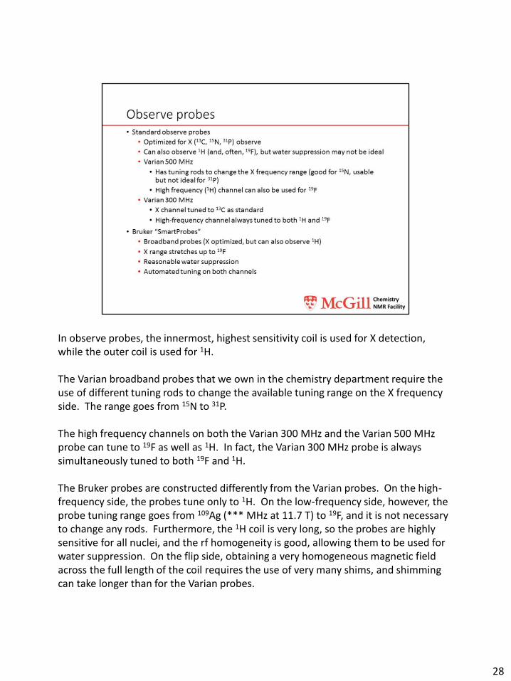
In observe probes, the innermost, highest sensitivity coil is used for X detection, while the outer coil is used for 1H.

The Varian broadband probes that we own in the chemistry department require the use of different tuning rods to change the available tuning range on the X frequency side. The range goes from 15N to 31P.

The high frequency channels on both the Varian 300 MHz and the Varian 500 MHz probe can tune to 19F as well as 1H. In fact, the Varian 300 MHz probe is always simultaneously tuned to both 19F and 1H.

The Bruker probes are constructed differently from the Varian probes. On the high-frequency side, the probes tune only to 1H. On the low-frequency side, however, the probe tuning range goes from 109Ag (*** MHz at 11.7 T) to 19F, and it is not necessary to change any rods. Furthermore, the 1H coil is very long, so the probes are highly sensitive for all nuclei, and the rf homogeneity is good, allowing them to be used for water suppression. On the flip side, obtaining a very homogeneous magnetic field across the full length of the coil requires the use of very many shims, and shimming can take longer than for the Varian probes.

28

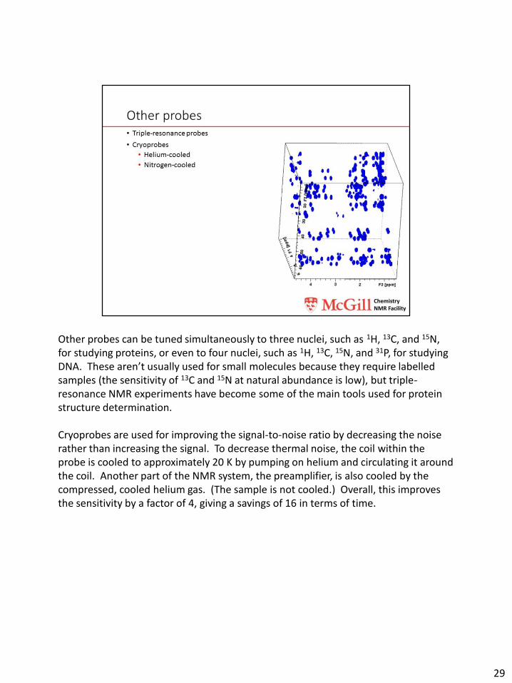
Other probes can be tuned simultaneously to three nuclei, such as 1H, 13C, and 15N, for studying proteins, or even to four nuclei, such as 1H, 13C, 15N, and 31P, for studying DNA. These aren’t usually used for small molecules because they require labelled samples (the sensitivity of 13C and 15N at natural abundance is low), but triple-resonance NMR experiments have become some of the main tools used for protein structure determination.

Cryoprobes are used for improving the signal-to-noise ratio by decreasing the noise rather than increasing the signal. To decrease thermal noise, the coil within the probe is cooled to approximately 20 K by pumping on helium and circulating it around the coil. Another part of the NMR system, the preamplifier, is also cooled by the compressed, cooled helium gas. (The sample is not cooled.) Overall, this improves the sensitivity by a factor of 4, giving a savings of 16 in terms of time.

29

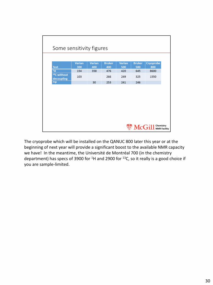
The cryoprobe which will be installed on the QANUC 800 later this year or at the beginning of next year will provide a significant boost to the available NMR capacity we have! In the meantime, the Université de Montréal 700 (in the chemistry department) has specs of 3900 for 1H and 2900 for 13C, so it really is a good choice if you are sample-limited.

30

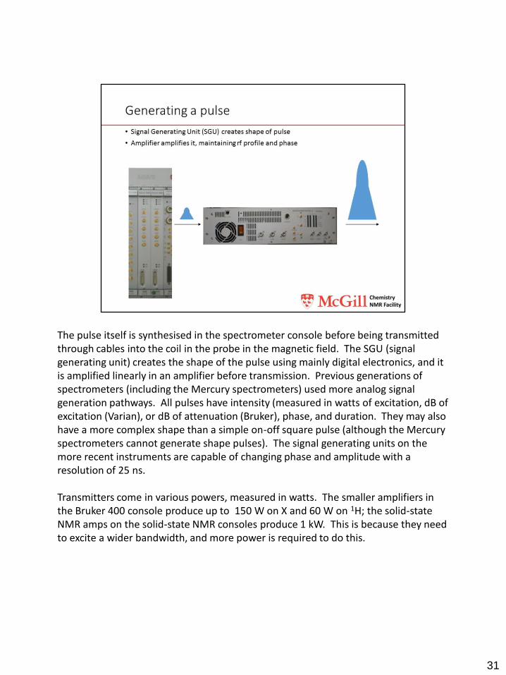
The pulse itself is synthesised in the spectrometer console before being transmitted through cables into the coil in the probe in the magnetic field. The SGU (signal generating unit) creates the shape of the pulse using mainly digital electronics, and it is amplified linearly in an amplifier before transmission. Previous generations of spectrometers (including the Mercury spectrometers) used more analog signal generation pathways. All pulses have intensity (measured in watts of excitation, dB of excitation (Varian), or dB of attenuation (Bruker), phase, and duration. They may also have a more complex shape than a simple on-off square pulse (although the Mercury spectrometers cannot generate shape pulses). The signal generating units on the more recent instruments are capable of changing phase and amplitude with a resolution of 25 ns.

Transmitters come in various powers, measured in watts. The smaller amplifiers in the Bruker 400 console produce up to 150 W on X and 60 W on 1H; the solid-state NMR amps on the solid-state NMR consoles produce 1 kW. This is because they need to excite a wider bandwidth, and more power is required to do this.

31

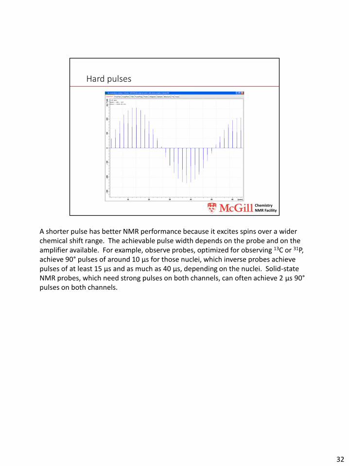
A shorter pulse has better NMR performance because it excites spins over a wider chemical shift range. The achievable pulse width depends on the probe and on the amplifier available. For example, observe probes, optimized for observing 13C or 31P, achieve 90° pulses of around 10 μs for those nuclei, which inverse probes achieve pulses of at least 15 μs and as much as 40 μs, depending on the nuclei. Solid-state NMR probes, which need strong pulses on both channels, can often achieve 2 μs 90°pulses on both channels.

32

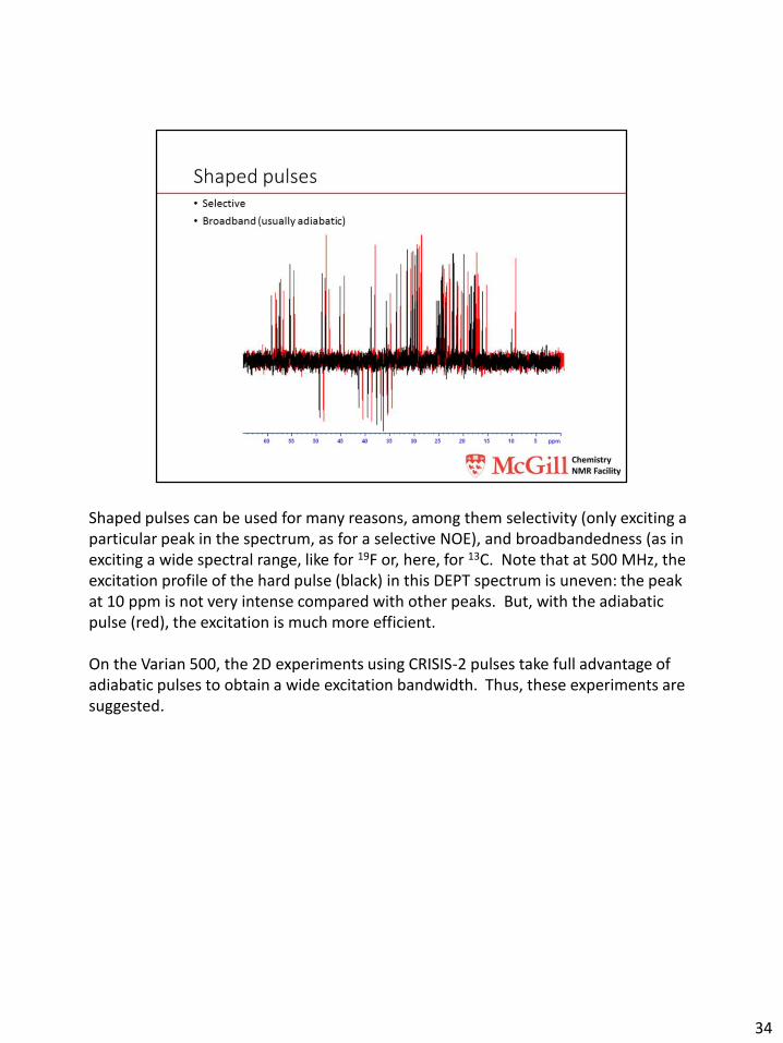
Shaped pulses can be used for many reasons, among them selectivity (only exciting a particular peak in the spectrum, as for a selective NOE), and broadbandedness (as in exciting a wide spectral range, like for 19F or, here, for 13C. Note that at 500 MHz, the excitation profile of the hard pulse (black) in this DEPT spectrum is uneven: the peak at 10 ppm is not very intense compared with other peaks. But, with the adiabatic pulse (red), the excitation is much more efficient.

On the Varian 500, the 2D experiments using CRISIS-2 pulses take full advantage of adiabatic pulses to obtain a wide excitation bandwidth. Thus, these experiments are suggested.

34

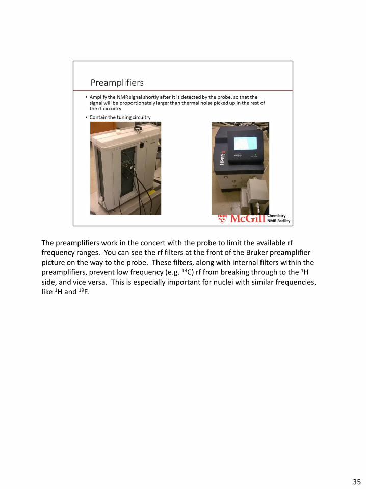
The preamplifiers work in the concert with the probe to limit the available rffrequency ranges. You can see the rf filters at the front of the Bruker preamplifier picture on the way to the probe. These filters, along with internal filters within the preamplifiers, prevent low frequency (e.g. 13C) rf from breaking through to the 1H side, and vice versa. This is especially important for nuclei with similar frequencies, like 1H and 19F.

35

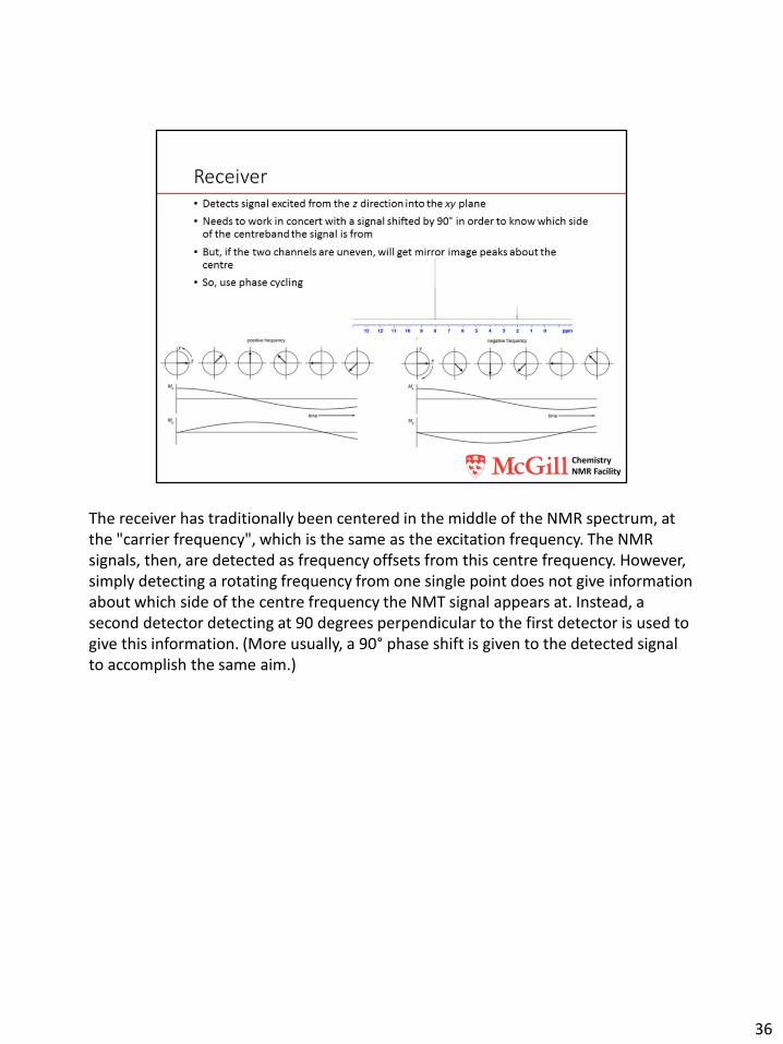
The receiver has traditionally been centered in the middle of the NMR spectrum, at the "carrier frequency", which is the same as the excitation frequency. The NMR signals, then, are detected as frequency offsets from this centre frequency. However, simply detecting a rotating frequency from one single point does not give information about which side of the centre frequency the NMT signal appears at. Instead, a second detector detecting at 90 degrees perpendicular to the first detector is used to give this information. (More usually, a 90° phase shift is given to the detected signal to accomplish the same aim.)

36

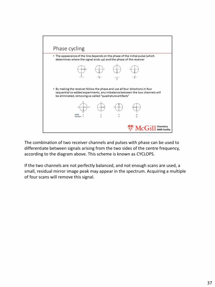
The combination of two receiver channels and pulses with phase can be used to differentiate between signals arising from the two sides of the centre frequency, according to the diagram above. This scheme is known as CYCLOPS.

If the two channels are not perfectly balanced, and not enough scans are used, a small, residual mirror image peak may appear in the spectrum. Acquiring a multiple of four scans will remove this signal.

37

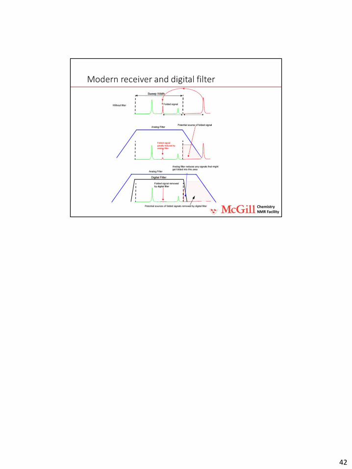
More modern receivers circumvent problems of receiver artifacts by acquiring with a significantly larger bandwidth of some megahertz. Thus, they do not need to be centered in the centre of the spectrum. Instead, a digital filter is used to reduce the spectrum to only the desired region.

38

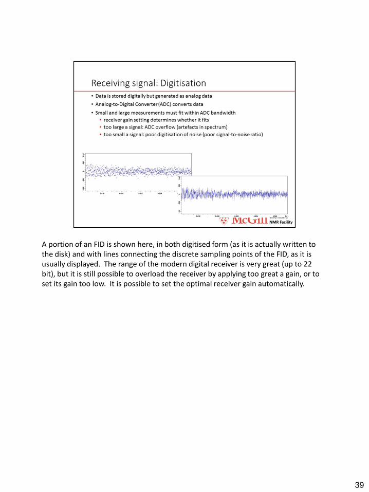
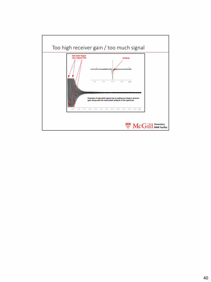
A portion of an FID is shown here, in both digitised form (as it is actually written to the disk) and with lines connecting the discrete sampling points of the FID, as it is usually displayed. The range of the modern digital receiver is very great (up to 22 bit), but it is still possible to overload the receiver by applying too great a gain, or to set its gain too low. It is possible to set the optimal receiver gain automatically.

39

40

41

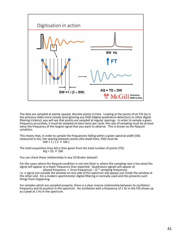
The data are sampled at evenly spaced, discrete points in time. Looking at the points of an FID (as in the previous slide) more closely (and ignoring any DQD (digital quadrature detection) or other digital filtering trickery), you will see that points are sampled at regular spacings. In order to sample a given frequency accurately, it must be sampled at least twice per cycle: the rate of sampling must be at least twice the frequency of the largest signal that you want to observe. This is known as the Nyquist condition.

This means that, in order to sample the frequencies falling within a given spectral width (SW, measured in Hz), the spacing between points (the dwell time, DW) must be

DW = 1 / ( 2 × SW )

The total acquisition time AQ is then given from the total number of points (TD):AQ = TD × DW

You can check these relationships in any 1D Bruker dataset!

For the cases where the Nyquist condition is not met (that is, where the sampling rate is too slow) the signal will appear at a lower frequency than expected. Quadrature signals will appear at

aliased frequency = (true frequency) – (2 * sampling frequency)i.e. a signal just outside the window on one side of the spectrum will appear just inside the window at the other end. On a modern spectrometer digital filtering is normally used and this prevents such things from happening.

For samples which are sampled properly, there is a clear inverse relationship between its oscillation frequency and its position in the spectrum. An oscillation with a frequency of 1 Hz in the FID shows up as a peak at 1 Hz in the spectrum.

42

43

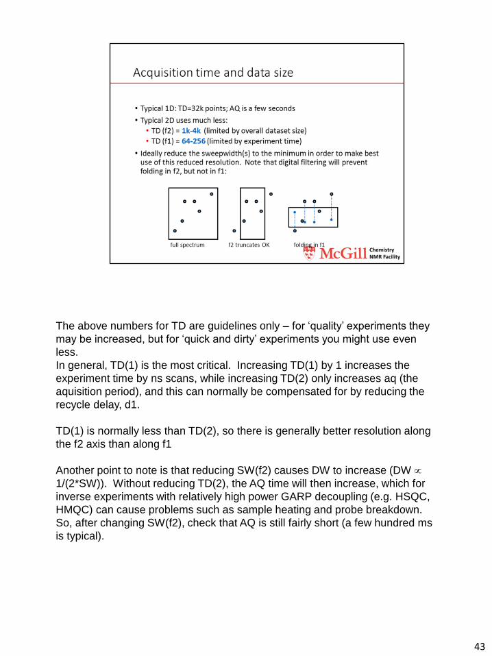
The above numbers for TD are guidelines only – for ‘quality’ experiments they

may be increased, but for ‘quick and dirty’ experiments you might use even

less.

In general, TD(1) is the most critical. Increasing TD(1) by 1 increases the

experiment time by ns scans, while increasing TD(2) only increases aq (the

aquisition period), and this can normally be compensated for by reducing the

recycle delay, d1.

TD(1) is normally less than TD(2), so there is generally better resolution along

the f2 axis than along f1

Another point to note is that reducing SW(f2) causes DW to increase (DW

1/(2*SW)). Without reducing TD(2), the AQ time will then increase, which for

inverse experiments with relatively high power GARP decoupling (e.g. HSQC,

HMQC) can cause problems such as sample heating and probe breakdown.

So, after changing SW(f2), check that AQ is still fairly short (a few hundred ms

is typical).

44

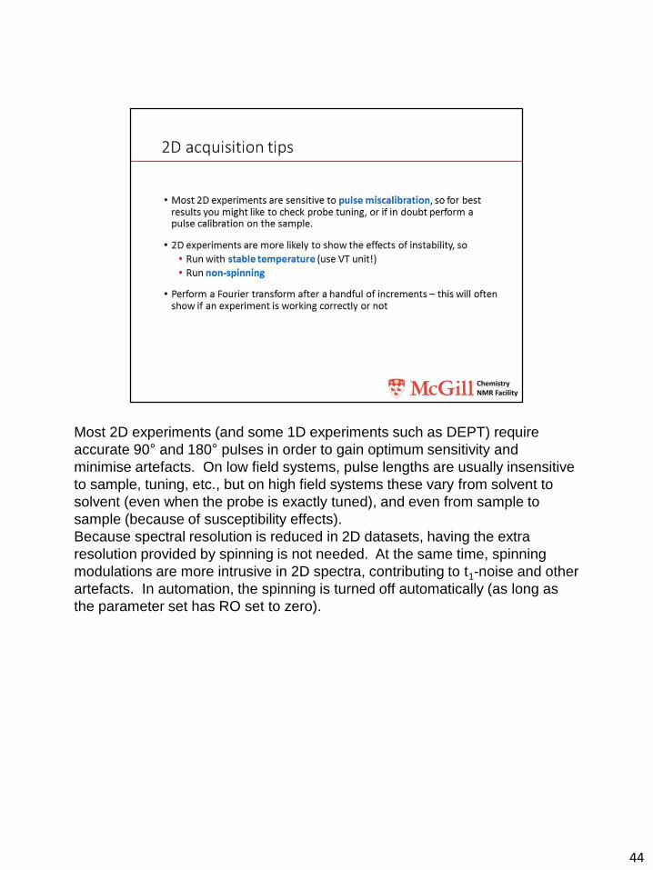
Most 2D experiments (and some 1D experiments such as DEPT) require

accurate 90° and 180° pulses in order to gain optimum sensitivity and

minimise artefacts. On low field systems, pulse lengths are usually insensitive

to sample, tuning, etc., but on high field systems these vary from solvent to

solvent (even when the probe is exactly tuned), and even from sample to

sample (because of susceptibility effects).

Because spectral resolution is reduced in 2D datasets, having the extra

resolution provided by spinning is not needed. At the same time, spinning

modulations are more intrusive in 2D spectra, contributing to t1-noise and other

artefacts. In automation, the spinning is turned off automatically (as long as

the parameter set has RO set to zero).

45

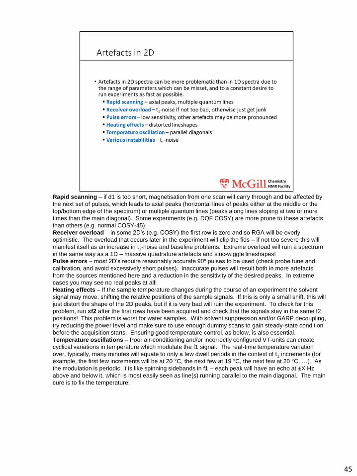
Rapid scanning – if d1 is too short, magnetisation from one scan will carry through and be affected by

the next set of pulses, which leads to axial peaks (horizontal lines of peaks either at the middle or the

top/bottom edge of the spectrum) or multiple quantum lines (peaks along lines sloping at two or more

times than the main diagonal). Some experiments (e.g. DQF COSY) are more prone to these artefacts

than others (e.g. normal COSY-45).

Receiver overload – in some 2D’s (e.g. COSY) the first row is zero and so RGA will be overly

optimistic. The overload that occurs later in the experiment will clip the fids – if not too severe this will

manifest itself as an increase in t1-noise and baseline problems. Extreme overload will ruin a spectrum

in the same way as a 1D – massive quadrature artefacts and sinc-wiggle lineshapes!

Pulse errors – most 2D’s require reasonably accurate 90º pulses to be used (check probe tune and

calibration, and avoid excessively short pulses). Inaccurate pulses will result both in more artefacts

from the sources mentioned here and a reduction in the sensitivity of the desired peaks. In extreme

cases you may see no real peaks at all!

Heating effects – If the sample temperature changes during the course of an experiment the solvent

signal may move, shifting the relative positions of the sample signals. If this is only a small shift, this will

just distort the shape of the 2D peaks, but if it is very bad will ruin the experiment. To check for this

problem, run xf2 after the first rows have been acquired and check that the signals stay in the same f2

positions! This problem is worst for water samples. With solvent suppression and/or GARP decoupling,

try reducing the power level and make sure to use enough dummy scans to gain steady-state condition

before the acquisition starts. Ensuring good temperature control, as below, is also essential.

Temperature oscillations – Poor air-conditioning and/or incorrectly configured VT-units can create

cyclical variations in temperature which modulate the f1 signal. The real-time temperature variation

over, typically, many minutes will equate to only a few dwell periods in the context of t1 increments (for

example, the first few increments will be at 20 °C, the next few at 19 °C, the next few at 20 °C, …). As

the modulation is periodic, it is like spinning sidebands in f1 – each peak will have an echo at ±X Hz

above and below it, which is most easily seen as line(s) running parallel to the main diagonal. The main

cure is to fix the temperature!

46

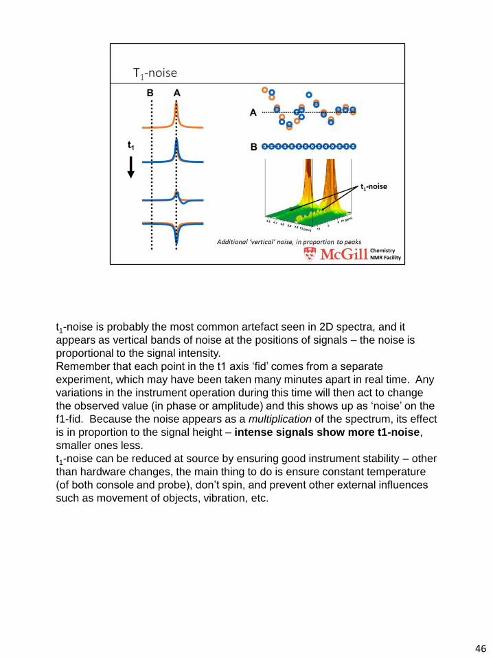
t1-noise is probably the most common artefact seen in 2D spectra, and it

appears as vertical bands of noise at the positions of signals – the noise is

proportional to the signal intensity.

Remember that each point in the t1 axis ‘fid’ comes from a separate

experiment, which may have been taken many minutes apart in real time. Any

variations in the instrument operation during this time will then act to change

the observed value (in phase or amplitude) and this shows up as ‘noise’ on the

f1-fid. Because the noise appears as a multiplication of the spectrum, its effect

is in proportion to the signal height – intense signals show more t1-noise,

smaller ones less.

t1-noise can be reduced at source by ensuring good instrument stability – other

than hardware changes, the main thing to do is ensure constant temperature

(of both console and probe), don’t spin, and prevent other external influences

such as movement of objects, vibration, etc.