What Can we Learn from Euro-Dollar Tweets? 1

Vahid Gholampour

Bucknell University

Eric van Wincoop

University of Virginia

NBER

July 14, 2017

1We gratefully acknowledge financial support from the Bankard Fund for Political Economy. We like

to thank seminar participants at the University of Virginia, Bucknell University, the Federal Reserve Bank

of Dallas, the Federal Reserve Bank of Richmond, the NBER Fall 2016 IFM Meeting, the University of

Lausanne and the Hong Kong Institute for Monetary Research for useful comments. We particularly

thank Laura Veldkamp for very helpful comments.

Abstract

We investigate what can be learned from 633 days of tweets that express opinions about the

Euro/dollar exchange rate. Relative to related literature using social media opinions to predict

stock prices, we make two methodological innovations. First, we develop a detailed lexicon used

by traders to translate verbal tweets into positive, negative and neutral opinions. We find that

individuals with a lot of followers can predict the direction of the exchange rate and have more

information than individuals with fewer followers. Second, we use a model with dispersed infor-

mation to extract more information from the tweets. The model allows us to consider a broader

set of moments involving Twitter Sentiment and exchange rates. Taking into account uncertainty

about estimated model parameters, the Sharpe ratio from a trading strategy based on Twitter

Sentiment can be computed with great precision. The Sharpe ratio outperforms that based on the

popular carry trade.

1 Introduction

Asset pricing models with asymmetric information commonly assume that information is widely

dispersed among traders.1 Traders have different information about future events or may interpret

the same information differently. All this information affects asset prices, which therefore in turn

provide a (noisy) looking glass into the dispersed private information in the market. With the

advent of the internet and social media, large numbers of people now go online to directly express

their opinions about the direction of asset prices.2 This leads to questions about the information

content of these online opinions and the profitability of trading based on this information.3 In this

paper we investigate what can be learned from Twitter by considering two and a half years of tweets

that express opinions about the Euro/dollar exchange rate. This is a natural choice as Twitter has

become a widely used platform to express opinions and the importance of private information for

the determination of exchange rates is well established through the FX microstructure literature.4

The paper makes two methodological contributions. The first relates to the classification of

tweets as positive, negative or neutral about the direction of the exchange rate. There is an

existing literature related to the stock market, reviewed below, which uses classification methods

that are not specific to financial markets and the language used by traders in financial markets.

We develop a “dictionary” of word combinations based on financial lexicon used by traders in

the Euro/dollar market to automate the interpretation of verbal tweets as positive, negative or

neutral.5 This leads to a measure of Twitter Sentiment. To extract even more information from

1See Brunnermeier (2001) for a review of the literature.2Opinion surveys existed before, but they were infrequent (usually monthly) and limited in scope.3There exists lots of anecdotal information suggesting that such information can be important. For example, on

August 13, 2013, Carl Icahn, an activist investor, tweeted about his large position in Apple. As a result, the stock

surged by over four percent in a few seconds. Almost two years later, on April 28, 2015, a data mining company

obtained Twitter’s quarterly earnings and posted it on Twitter before the scheduled release time. Twitter’s stock

plummeted by twenty percent and trading was halted by the NYSE.4The seminal contribution by Evans and Lyons (2002) established a close relationship between exchange rates

and order flow, with the latter seen as aggregating private information. Reviews of the FX microstructure literature

can be found in Evans (2011), Evans and Rime (2012), King, Osler and Rime (2013) and Lyons (2001).5We do not consider other currency pairs as a lot of the tweets are in different languages. But the overall method

described here can certainly be applied to other languages and currency pairs.

1

the tweets, we separately consider Twitter Sentiment from accounts with a lot of followers (at

least 500) and accounts with fewer followers (less than 500).

We look at three aspects of the data to evaluate information content. The first consists of

directional moments to see if tweets are able to predict the direction of the subsequent change

in the exchange rate. The second consists of predictability regressions. These regress exchange

rate changes over horizons from 1 day to 3 months on lagged Twitter Sentiment. The third is the

Sharpe ratio from a trading strategy based on Twitter Sentiment. Three conclusions can be drawn.

First, all three types of evidence indicate that the group with a lot of followers is more informed

than the group with fewer followers. Second, individuals with a lot of followers are able to predict

the direction of the subsequent change in the exchange rate in a way that is strongly statistically

significant. However, even for the group with a lot of followers, predictability coefficients are not

statistically different form zero and the Sharpe ratio is very imprecisely measured (could be very

large or very small).

Our sample consists of 633 trading days (two and a half years). The sample is long enough

to confirm that the group with a lot of followers has useful information that helps predict the

direction of the exchange rate change. But it is not long enough to predict the magnitude of the

subsequent exchange rate change or to show that a trading strategy based on Twitter Sentiment

is profitable. This is perhaps not surprising as opinions are only directional and it is well known

since Meese and Rogoff (1983a,b) that the exchange rate is close to a random walk.

Our second methodological contribution uses theory to extract more information from the data.

The use of a model with dispersed information allows us to learn from other aspects of the Twitter

Sentiment data, such as sentiment volatility, disagreement among agents, the contemporaneous

relationship between exchange rate changes and Twitter Sentiment and the correlation between

Twitter Sentiment of both groups. Imposing structure through a model leads to a much more

precise estimate of the Sharpe ratio. We find the Sharpe ratio to be high, especially for the group

with a lot of followers, and precisely measured. The Sharpe ratio even outperforms the popular

carry trade strategy.

The results based on the model are obviously under the assumption that the model is correct.

No model is exactly correct, but we show that the model cannot be rejected by the data and

2

does a good job in matching moments in the data. The model assumes that agents form opinions

based on private signals about future fundamentals, as well as public information in the form of

current and past macro fundamentals and exchange rates. The model is an extension of a noisy

rational expectation (NRE) model for exchange rate determination developed by Bacchetta and

van Wincoop (2006), from here on BvW. We extend the model of BvW to allow for two categories

of agents, referred to as informed and uninformed traders. They both receive private signals, but

informed traders receive higher quality private signals.6

The information structure in the model is defined by the precision of the signals of both groups

of agents, the horizon of future fundamentals over which they receive signals, the relative size of

the informed group and the known processes of observed fundamentals and unobserved noise

shocks. Importantly, the model itself does not impose anything regarding the information quality

of both private and public information. Dependent on model parameters, both private and public

information may be very valuable or entirely useless. There is no presumption that the agents

have useful information of any kind.

There are no tweets in the model. Tweets are interpreted as the expression of an opinion by

a subset of agents. We use cutoffs for expectations to obtain a theoretical Twitter Sentiment of

+1 (expected Euro appreciation), -1 (expected Euro depreciation) or 0 (neutral) for each agent.

This allows us to connect to the data, where we use our financial lexicon to assign the same three

values. The cutoffs for expectations in the theory are such that the unconditional distribution

across the three values in the model corresponds to that in the data.

After estimation with the Simulated Method of Moments, the model is used to evaluate pre-

dictability and Sharpe ratios. It should be emphasized that predicting exchange rates is no easy

matter. The exchange rate can be written as the present discounted value of future fundamentals.

Engel and West (2005) show that reasonable estimates of the discount rate (close to 1) imply

near-random walk behavior as seen in the data. We parameterize the model to obtain a discount

rate consistent with Engel and West (2005). Predictability will therefore always be limited, no

6The distinction between informed and uninformed agents is actually quite common in NRE models. A good

example is Wang (1994). But in those models it is assumed that uninformed agents do not receive any private

signals. We instead assume lower quality private signals, with the precision of the signals to be estimated.

3

matter the quality of the information.

Although we are not aware of other applications to the foreign exchange market, the paper

relates to a literature that has used messages from social media and the internet to predict stock

prices. This usually involves short data samples of no more than a year. Results are based on

regressions of stock price returns on either “mood” states (like hope, happy, fear, worry, nervous,

upset, anxious, positive, negative) or an opinion about the direction of stock price changes (along

the line of positive, negative or neutral). Predictability is considered at most a couple of days

into the future. Papers focusing on mood states, like Bollen et.al. (2011), Zhang et.al. (2011),

Mittal and Goel (2012) and Zhang (2013), use an entire sweep of all Twitter messages, or random

sets of messages, rather than messages specifically related to financial markets.7 Some of the

literature prior to Twitter did focus specifically on financial messages. These include Antweiler

and Frank (2004) and Das and Chen (2007), who use message boards like Yahoo!Finance, and

Dewally (2003), who uses messages from newsgroups about US stocks. Evidence of predictability

in most of these papers is limited at best.

As emphasized above, our approach is methodologically different from this literature in two

key ways. First, the literature has not employed financial jargon used by traders to classify

messages. Most of the literature uses supervised machine-based learning classifiers that are not

specific to financial markets at all, such as the Naive Bayes algorithm. Tetlock (2007) has used

a dictionary approach to consider the ability of verbal text to predict stock prices. But it is

based on the Harvard IV dictionary that is not specifically related to financial news.8 Second, the

existing literature has not used theory to extract information from social media opinions related

to financial markets.

The remainder of the paper is organized as follows. In Section 2 we describe the Twitter data

and methodology used to translate opinionated tweets about the Euro/dollar into positive (+1),

negative (-1) and neutral (0) categories. We consider what can be learned from this Twitter Sen-

timent data through directional moments, predictability regressions and Sharpe ratios. In Section

7Mao et.al. (2015) uses an entire sweep of messages to search for the words “bullish” and “bearish” to classify

tweets.8Moreover, it is applied to WSJ articles as opposed to the diverse opinions expressed by a broad set of individuals

on message boards and social media.

4

3 we describe the NRE model of exchange rate determination used to extract more information

from the data. Section 4 discusses the empirical methodology in connecting the model to the data

and Section 5 presents the results. Section 6 concludes.

2 Data and Methodology

The objective is to translate daily verbal tweets that express opinions about the dollar/Euro

exchange rate into a numerical measure of Twitter Sentiment (TS) that reflects expectations about

the future direction of the exchange rate. After a discussion about possible biases related to the

reasons for tweeting, we describe how we use a dictionary of financial lexicon to measure Twitter

Sentiment. We then use the results to provide evidence from directional moments, predictability

regressions and Sharpe ratios without any guidance from theory. We also discuss a broader set of

moments involving Twitter Sentiment and exchange rates that will be confronted with the theory

in Section 5.

2.1 Why Individuals Tweet

Before we describe Twitter data and the steps of constructing Twitter Sentiment, a brief discussion

of potential motivations by individuals for tweeting their outlook is in order. There are two

potential ways in which such motivations can generate biases that can affect the analysis. The

first bias occurs when individuals are motivated to tweet something that does not correspond to

their actual beliefs. The second bias occurs when individuals are more or less likely to tweet in a

way that is correlated with their outlook for the exchange rate.

The first bias is not likely to be much of a concern, for various reasons. First, it is hard to think

of a reason to tweet the opposite of one’s belief. Even if the objective of a tweet is to steer the

market in a certain direction, there is little reason to steer it in a direction opposite to one’s beliefs,

especially if the individual has a stake in the outcome. Second, the market for the Euro-dollar

currency pair is one of the most liquid financial markets in the world, so few individuals would

be able to influence the exchange rate through malicious tweets. Finally, the self-provided user

descriptions provide some information about the motivation for the tweets. A significant fraction of

5

accounts with a lot of followers are controlled by individuals or businesses that provide investment

research services. They occasionally tweet their future outlook to showcase their research and

gain more subscribers for their business. Businesses have no incentive to tweet an opinion that

is in contradiction with their internal research because misleading the followers could hurt their

reputation.

The second type of bias occurs if people are more likely to tweet when they have particularly

strong beliefs about the direction of the exchange rate. This can bias the average opinion. If this

is the case, the percentage of neutral tweets is inversely related to the total number of tweets.

To test this, we separate the days into the bottom and top 25 percent in terms of the number of

tweets. For days with few tweets (bottom 25 percent), we classify 31.7 percent as neutral tweets.

For days with a large number of tweets (top 25 percent), 29.7 percent are classified as neutral

tweets. If there is any bias, it is clearly not very large.9

2.2 Overall Approach to Computing Twitter Sentiment

It is important to describe in some detail how we translate verbal tweets into a numerical Twitter

Sentiment. We have used Twitter’s publicly available search tools since October 9, 2013, to

download the tweets in real time every half an hour. Every tweet includes the user name, the

number of followers of the individual who posted the tweet, as well as the exact time and date

that the tweet was posted. We start with all Twitter messages that mention EURUSD in their

text and are posted between October 9, 2013 and March 11, 2016. There are on average 578 such

messages coming from distinct Twitter accounts per day, for a total of 268,770 tweets.10 However,

the bulk of these messages do not include an opinion about the future direction in which the

exchange rate will move. For example, many mention changes in the Euro/dollar exchange rate

that have already happened or advertise a link to a web site discussing the Euro/dollar exchange

rate.

9We find the same if we separate the tweets into those with more than the average number of tweets (top 50

percent) and those with fewer than the average number of tweets (bottom 50 percent). We also get similar results

when we separately consider tweets from those with a lot of followers and those with few followers, as we will do

below.10Here we count multiple tweets from the same account during a day as one EURUSD tweet.

6

The next step then is to look for opinionated tweets that express a positive, negative, or

neutral outlook about the direction of the exchange rate. The exchange rate is dollars per Euro,

denoted st in logs. A positive sentiment therefore means an expected Euro appreciation, while a

negative sentiment indicates an expected Euro depreciation. A neutral outlook indicates a lack of

conviction or dependency of the outlook on the outcome of a future event. Numerically we measure

a positive outlook as +1, a negative outlook as -1 and a neutral outlook as 0. Unfortunately the

tweets are not sufficiently precise to capture further gradations. The tweets are also not precise

about the horizon of the expectation, an issue to which we return in Section 4 when discussing

the connection to the theory.

In order to identify such opinionated tweets, and categorize them as positive, negative or

neutral, we search for many different word combinations. A number of recent papers, such as

Tetlock (2007) and Da, Engelberg, and Gao (2015), use Harvard IV-4 dictionary and word counting

to conduct text analysis. This approach is shown to be effective in analyzing the content of

financial articles and Google search words. However, the dictionary is not structured to capture

the vocabulary used by investors. Since opinionated tweets about the exchange rate are usually

posted by investors, there is a certain type of lexicon that is found in most of these tweets. We

identify this lexicon by studying large numbers of tweets. We then go through several rounds

of improving our dictionary of financial lexicon by comparing the results from the automated

classification to that based on manual classification. We stopped making further changes when

we found only very few errors after manually checking 5000 tweets. We describe this dictionary

further below.

A day is defined as the 24 hour period that ends 12 noon EST. This corresponds well to our

data on exchange rates as the Federal Reserve reports daily spot exchange rates at 12PM in New

York. We allow only one opinion for each Twitter account on any given day to ensure that the

measure of sentiment is not dominated by few individuals who express their opinion multiple

times. We are not interested in intra-day price fluctuations. When there are multiple tweets from

one account during a day, we only use the last tweet on that day.11

11On average 16.9% of tweets counted this way are from accounts from which multiple tweets were sent during

a day.

7

There are on average 43.5 such opinionated tweets per day, for a total of 27,557 during our

sample. Therefore only about 8.5% of all tweets with the word EURUSD are opinionated tweets.

The 27,557 opinionated tweets come from 6,236 separate accounts, implying an average of 4.4

tweets per account over the entire 633 day period of our sample. The opinions are therefore from

a very diverse set of individuals as opposed to the same individuals repeating their opinions day

after day. If the 27,557 tweets all came from individuals tweeting every day, there would have

been only 43 separate accounts. We are clearly capturing a far more dispersed group of people

expressing opinions.

2.3 Financial Lexicon

Tables A1 and A2 in Appendix A provide the list of all word combinations used to identify tweets as

positive, negative or neutral. As can be seen, there are various ways that a tweet can be identified

to be in one of the three categories. It might involve simply the combination of certain words,

or the combination of some words together with the explicit absence of other words (positive and

negative word combinations).12 In order to provide some perspective, Table 1 provides examples of

tweets and how they are categorized. The words in the tweet used to identify them are underlined.

In Table 1, the first tweet under the positive category is identified as positive because investors

use “higher high” to describe an uptrend in the price charts. In this example, using the individual

words to extract the opinion could be misleading because the word “risk” might be interpreted as

a negative word and the word “high” by itself is not enough to identify a positive opinion because

investors use the word combination “lower high” to describe a downtrend. The first tweet under

the neutral category is placed in this category because the words “might” and “sell” indicate lack

of a definitive decision. Finally, the first tweet under the negative category is classified as bearish

because the words “further” and “fall” indicate that the individual expects Euro to depreciate

further against the dollar. We should note that the tweet mentions the word “bullish,” which is

a positive word. However, as mentioned earlier, we require the existence of certain words in the

12It is possible that a tweet has word combinations in more than one category. We classify a tweet with both

positive and neutral word combinations as positive. Similarly, a tweet with negative and neutral words combinations

is classified as negative. A tweet with both positive and negative word combinations is classified as neutral.

8

absence of other words to place a tweet in a category. In this example, the tweet is not identified

as positive because a tweet should mention “bullish” and not mention “missing” to be placed in

the positive category. This tweet is another example that highlights the significance of using word

combinations instead of words to classify the opinionated tweets.

2.4 Separation by Number of Followers

We separate the opinionated tweets into those coming from individuals with at least 500 followers

from those that have fewer than 500 followers. The idea is that those with more followers may be

better informed investors. There are 4496 accounts with less than 500 followers and 2007 accounts

with more than 500 followers.13 Figure 1 shows the distribution of the number of followers,

separately for accounts with more and less than 500 followers. For those with less than 500

followers, a large number has fewer than 50 followers. Of those that have more than 500 followers,

725 accounts have between 500 and 1000 followers, while 1282 accounts have more than 1000

followers.

We will see that the evidence strongly bears out the suspicion that individuals with a lot of

followers are more informed. It should be noted that those with at least 500 followers are not

famous people outside of the financial world, like movie stars who happen to tweet about the

Euro/dollar exchange rate. Typical examples are brokers, technical analysts, financial commenta-

tors and people with research websites. One would expect these individuals to be well informed.

From hereon we will simply refer to these two groups as informed and uninformed investors.

With this split, the daily average of opinionated tweets posted by informed and uninformed

investors is respectively 21 and 22, so that we have a similar number of tweets in both groups.

It may be the case that for example individuals with 1000 followers are even more informed than

those with 500 followers, but splitting the data into more than 2 groups based on followers has the

disadvantage of lowering the number of daily tweets per group. Figure 2 shows the distribution of

daily tweets for both groups. It varies a lot across days. The standard deviation of the number

13The total of these accounts is a bit larger than the 6236 mentioned above. This is because 267 individuals

switch between both groups during the sample. We categorize the tweets each day based on the number of followers

on that day.

9

of daily tweets is respectively 12.7 and 13.2 for the informed and uninformed. Since the average

number of daily tweets of both groups is about the same, and there are fewer accounts from

informed individuals, the average number of tweets per account during the sample is larger for

informed than uninformed individuals, respectively 6.6 and 3.1.

We will denote the numerical Twitter Sentiment during day t by individual i from the informed

group as TSI,it . Analogously, when the individual is from the uninformed group it is denoted as

TSU,it . Figure 3 shows the distribution of the three values (-1, 0 and 1) that individual Twitter

Sentiment of both groups takes across the entire sample. Especially for the informed group the

percentage of negative values is a bit larger than the percentage of positive values. This is because

the Euro depreciated by 21% during this particular sample.

For each of the two groups (informed and uninformed) we also construct a daily Twitter

Sentiment Index. It is computed by taking the simple average of the numerical Twitter Sentiment

across individuals during a day. We denote this as TSIt and TSU

t for respectively informed and

uninformed investors on day t. So

TSjt =

1

njt

njt∑

i=1

TSj,it (1)

where j = I, U is the group and njt is the number of opinionated tweets on day t in group j. There

are no tweets during 2 days in the sample for the informed group and 3 days for the uninformed.

We set the index to 0 for those days. Figure 4 shows the distribution of the daily Twitter Sentiment

Index for both groups.

We now turn to evidence on the information content of tweets from directional moments,

predictability regressions and the Sharpe ratio of a trading strategy based on the Twitter Sentiment

Index.

2.5 Directional Moments

Table 2 reports directional moments, which capture how well tweets predict the subsequent di-

rection of the exchange rate change. These moments are computed as follows. Consider a tweet

by agent i of group j on day t. We look at how well it can forecast the direction of the exchange

rate change over the next month, two months and three months. For example, st+40 − st is the

10

change in the exchange rate over the next two months as there are about 20 trading days in a

month. If TSjit = 1 and the subsequent exchange rate change is positive (negative), we assign

the tweet a +1 (-1). Similarly, if TSjit = −1 and the subsequent exchange rate change is positive

(negative), we assign the tweet a -1 (+1). So +1 will be assigned if the direction is consistent

with the Twitter Sentiment and -1 if the direction is inconsistent with the sentiment. A zero is

assigned if TSjit = 0, so that there is no directional opinion. We then take the average across all

the tweets in the sample. A positive number suggests that the direction was more often correct

than wrong, while a negative number suggests the opposite.

Standard errors are computed through bootstrapping. Holding the number of tweets equal to

njt for group j, we randomly draw, with replacement, nj

t values of TSj,it for day t. After doing so

for 633 days, we compute the directional moments, using the observed subsequent exchange rate

changes. We repeat this 1000 times to compute the standard error of the directional moments.14

As can be seen in Table 2, the moments for the informed group are highly significant. For the

one month, two month and three month subsequent exchange rate change the directional moment

is respectively 3.4, 8.1 and 4.3 standard errors away from zero. This is strong evidence that there

is valuable information content in the tweets of the informed group. The same cannot be said of

the uninformed group, where the moments are slightly negative. Figure 6 reports the directional

moments over all horizons from 1 day to 60 days (3 months) for the informed, as well as the 95

percent confidence band. The directional moments peak just short of two months (40 days). That

is the horizon over which the informed appear to have most information.

2.6 Predictability Regressions

Directional moments themselves do not tell us if Twitter Sentiment is a good predictor of the

actual magnitude of subsequent exchange rate changes. This is important if we wish to use Twitter

Sentiment for trading purposes, where actual returns matter rather than the sign of the return.

To this end we regress the exchange rate change st+m − st on the Twitter Sentiment Index. We

14Results are virtually identical when we draw, with replacement, from all observations (TSj,it , st+m − st) where

m is the forecast horizon. In that case the number of tweets from a particular day may differ from the actual

number of tweets in the original sample.

11

do this again for one month, two month and three month horizons (m = 20, m = 40 and m = 60),

but also for a one-day horizon (m = 1). The one-day horizon is useful as we will report Sharpe

ratios from a strategy based on Twitter Sentiment that is based on daily returns. We regress

either on Twitter Sentiment TSjt at the start of the forecasting period or on Twitter Sentiment

on each of the last 5 days before the forecasting period (TSjt through TSj

t−4). The results from

these predictability regressions are reported in Tables 3 and 4 for respectively the informed and

uninformed groups. The regressions are based on overlapping data intervals with Newey-West

standard errors in parenthesis.15 The bottom of the table reports the p-value associated with the

F-test of zero coefficients on all lags of the Twitter Sentiment index.

There is no evidence of predictability as the coefficients are insignificant. The only exception

is for the one-day horizon for uninformed agents when we use 5 days of Twitter Sentiment. But

in that case the significant coefficients have the wrong sign. This lack of predictability suggests

that the sample is too short to evaluate the ability of Twitter Sentiment to predict the subsequent

exchange rate change.

There is evidence though that the two groups are different. To test the null hypothesis that

the predictability is the same for both groups, for each day we bootstrap the observations TSUit

for the uninformed to create a new Twitter Sentiment Index for the uninformed and repeat the

predictability regressions. Repeating this 1000 times, we find that only one time (0.1%) at least 22

of the 24 regression coefficients are positive, as we see for the informed in Table 3. The difference

between both groups is also consistent with the results from the directional moments.

2.7 Sharpe Ratio Trading Strategy Based on Twitter Sentiment

Table 5 reports the Sharpe ratio of a trading strategy based on Twitter Sentiment of both groups.

For group j we take a position of TSjt dollars in Euro denominated bonds and−TSj

t dollars in dollar

denominated bonds. We therefore go long in Euros when Twitter Sentiment is positive (expected

Euro appreciation) and short in Euros when Twitter Sentiment is negative. It is important that

positions are proportional to Twitter Sentiment as a stronger Twitter Sentiment implies more

15Following Andrews (1991), we use m+ 1 lags for the Newey-West standard errors.

12

confidence that the exchange rate will go in a certain direction. The return from this strategy is

TSjt (st+1 − st + i∗t − it) (2)

Here it and i∗t are overnight dollar and Euro interest rates. We use overnight Libor rates for both,

obtained from the St. Louis Fed.16

Table 5 shows that the Sharpe ratio is 1.09 for the informed group and -0.19 for the uninformed

group. These are annualized Sharpe ratios based on daily returns. We annualize by multiplying

by the square root of 250, the number of trading days in a year. GMM standard errors and 95%

confidence intervals are shown as well. While the Sharpe ratio of 1.09 for the informed group is

attractive, it has a large standard error of 0.6. The 95% confidence interval is therefore very wide,

ranging from -0.09 to 2.27. We can therefore say very little about the merits of trading based on

Twitter Sentiment. This is consistent with the results we reported for exchange rate predictability

in Tables 3 and 4. For the uninformed group the 95% confidence interval is [-1.41,1.03]. While

the point estimate of -0.19 suggests that there is no information content in Twitter Sentiment of

the uninformed, with the wide confidence interval we cannot rule out that the true Sharpe ratio

is near 1.

There is again evidence though that the two groups are different. The difference in Sharpe

ratios is statistically significant. Under the null hypothesis that the two groups are the same, we

draw nIt times from the set of nU

t tweets of the uninformed on day t to create samples with the

same number of tweets as we have for the informed. For each sample we recompute the Sharpe

ratio. The standard error of 0.57 obtained this way implies that the difference of 1.28 in the

Sharpe ratios of the informed and uninformed is statistically significant.

2.8 Summary Model Free Evidence

So far we have looked at the data without imposing the structure of a model. All three types

of evidence we looked at (directional moments, predictability regressions and Sharpe ratios) con-

firm that tweets from the informed group have more information content than tweets from the

16The dollar overnight Libor rate is the series USDONTD156N. The Euro overnight Libor rate is the series

EURONTD156N.

13

uninformed group. There is strong evidence that the informed are able to predict the direction

of the exchange rate change. However, we have not been able to establish that they can predict

the magnitude of the exchange rate change. Related to that, the Sharpe ratio is very imprecisely

measured. These findings are not surprising given the limited data sample of two and a half

years, the directional nature of the tweets and the near-random walk behavior of exchange rates.

The fact that there is evidence of information content at all (through the directional moments) is

encouraging.

In order to learn more about the information content of the tweets, and the Sharpe ratio from

a trading strategy based on the tweets, we will impose structure through a model. This allows us

to consider a variety of other aspects of the data.

2.9 Moments for Model Evaluation

In Section 5 we will confront the model of Section 3 with a variety of data moments involving

TSI,it , TSU,i

t , TSIt , TSU

t and st. These moments are reported in the first column of Table 7. The

first 3 moments relate to the Twitter Sentiment indices. The first and second moment are the

variance of TSIt and TSU

t .17 The variance is a bit higher for informed individuals (0.098 versus

0.068). This is not surprising as new information leads to changes in expectations. Figure 4

illustrates this graphically. Average opinions in the uninformed group are more centered towards

the neutral 0, while the informed group shows a wider distribution. The third moment is the

correlation between the TS index of informed and uninformed agents, which is 0.44. This suggests

a significant common component in the average opinions of both groups.

The next two moments are disagreement moments, which relate to the extent to which opinions

differ among individuals during a particular day. They are the average across the 633 days of the

cross sectional variance of TSI,it and TSU,i

t across the individuals in that group. We again focus

on the variance for easier comparison to the model. We do not include the few days for which

the number of tweets is 0 or 1.18 Unsurprisingly, the average difference in opinion is a bit larger

17As we will discuss in Section 4, in the model the average variance of Twitter Sentiment is easier to compute

than the average standard deviation. That is why we use the variance in the data as well.18There are 6 days during which the number of tweets is 0 or 1 for the informed group and 5 days for the

uninformed group.

14

for uninformed individuals. This is also illustrated in Figure 5, which shows the distribution of

the daily cross sectional variance for both groups. The distribution of uninformed individuals is

clearly to the right of that distribution of informed individuals.

The next eight moments capture the correlation between Twitter Sentiment and future ex-

change rate changes. We consider the correlation of the Twitter Sentiment index with the change

in the exchange rate over the next 1, 20, 40 and 60 trading days for both informed and uninformed

groups. The correlations are positive for the informed group, but negative for the uninformed

group. As we will see in the model, these moments can vary a lot across different 633-day sam-

ples even when there is economically significant predictability. These correlations by themselves

therefore only provide limited information.

The next six moments are the directional moments described in Section 2.6 over 20, 40 and

60 days for the informed and uninformed groups. As discussed, these moments suggest significant

information content for the informed group.

The next two moments are the contemporaneous correlation between the weekly Twitter Sen-

timent index and weekly changes in the exchange rate. The weekly Twitter Sentiment Index TSjw

is defined as the average of the daily Twitter Sentiment Index over five trading days in a week.

The correlation is 0.26 for the informed and -0.01 for the uninformed group.

Finally, the last three moments are the standard deviation and autocorrelation of the daily

change in the exchange rate and the autocorrelation of the weekly change in exchange rate. The

standard deviation of the daily change in the exchange rate is in percent, so it is 0.57%=0.0057.

The daily and weekly autocorrelation are 0.003 and 0.008 respectively, reflecting the near random

walk aspect of the exchange rate.

3 Model Description

3.1 Some Preliminaries

In general agents have many different types of public and private information. Private information

may be related to different research findings, talking to different people in the market, reading

different financial news or perhaps even being exposed to different tweets or other social media

15

opinions. In the model all of this is captured by private signals that agents receive about future

fundamentals. In addition agents have public information in the form of macroeconomic data and

the exchange rate (including lags).

Three aspects of the model should be emphasized. First, we assume that agents rationally

process all public and private information to form expectations. Second, we make no a priori as-

sumption about the information quality. As we discuss further below, we leave open the possibility

that both public and private signals contain no useful information about the future. Even when

information is valuable, expectations about future macro fundamentals will be affected by random

private signal errors that are unrelated to future exchange rate changes. Third, the concept of a

“tweet” does not exist within the model. Tweets in reality are just an expression of a belief about

the direction of the exchange rate by a subset of agents. In the next section we will relate expec-

tations of exchange rate changes that exist in the model to directional beliefs expressed through

tweets.

The model is an extension of BvW along one dimension. In BvW all agents receive different

private signals, but the quality of these signals is identical in that the variance of the signal errors

is equal across all agents. In the extension developed here we assume that there are two groups

of agents, which we refer to as informed and uninformed. They are modeled in the same way,

except that the informed agents have higher quality private signals. The variance of signal errors

is smaller for informed agents. We will be relatively brief in the description of the model as BvW

develop the micro foundations and provide further details.

3.2 Model Equations

The model focuses on the demand for Foreign bonds. Let bI,iF,t and bU,iF,t be the demand for Foreign

bonds by informed and uninformed agent i. There is a continuum of such agents, with i ∈ [0, n]

for informed agents and i ∈ [n, 1] for uninformed agents. Since Foreign bonds are in zero net

supply, the market clearing condition is∫ n

0

bI,iF,tdi+

∫ 1

n

bU,iF,tdi = 0 (3)

16

Portfolio demand by agents is

bI,iF,t =EI,i

t st+1 − st + i∗t − itγσ2

I

− bI,it (4)

bU,iF,t =EU,i

t st+1 − st + i∗t − itγσ2

U

− bU,it (5)

Portfolio demand has two components. The first depends on the expected excess return on the

Foreign bonds, divided by the product of absolute risk aversion γ and the variance of the excess

return.19 st is the log exchange rate (Home currency per unit of Foreign currency), it and i∗t

are the Home and Foreign nominal interest rates. The variance of st+1 is respectively σ2I and σ2

U

for informed and uninformed agents. The computation of first and second moments of st+1 is

discussed below.

The second term in the portfolio is unrelated to expected returns. In BvW it represents a

hedge against non-asset income. In the literature it has alternatively been modeled as noise trade

or liquidity trade. What matters is their aggregate across agents:

bt =

∫ n

0

bI,it di+

∫ 1

n

bU,it di (6)

for which we assume an AR process:

bt = ρbbt−1 + εbt (7)

where εbt ∼ N(0, σ2b ). bt represents the noise that is present in all noisy rational expectations mod-

els. In equilibrium the exchange rate will be affected by both shocks to bt and private information

about future fundamentals. By assuming that bt is unobservable (only its AR process is known),

the equilibrium exchange rate will not reveal the aggregate of private information in the market.

We also follow BvW by assuming that bj,it (j = I, U) contains no information about the average

bt.

Standard money demand equations are assumed:

mt = pt + yt − αit (8)

m∗t = p∗t + y∗t − αi∗t (9)

19The effect of allowing for different rates of risk-aversion of the two groups is analogous to changing n.

17

mt is the log money demand, which must equal the log of money supply. yt is log output. pt is the

log price level. The analogous variables for the Foreign country are denoted with a * superscript.

Using PPP (pt = st + p∗t ), subtracting these equations yields

it − i∗t =1

α(st − ft) (10)

where ft = (mt −m∗t ) − (yt − y∗t ) is the traditional fundamental. Since the exchange rate is an

I(1) variable in the data, the fundamental is assumed to be I(1) as well. We assume

ft − ft−1 = ρ(ft−1 − ft−2) + εft (11)

where εft ∼ N(0, σ2f ). The fundamental and its process are known to all agents. We will also write

the fundamental as ft = D(L)εft , where D(L) =∑∞

i=1 diLi−1 is an infinite order polynomial in

the lag operator L, with di = 1 + ρ + ... + ρi−1. Agents know the values of all current and past

fundamental innovations.

Denote EIt st+1 =

∫ n

0EI,i

t st+1di/n as the average expectation across informed agents and anal-

ogously EUt st+1 for uninformed agents. Substituting (4), (5) and (10) into the market clearing

condition (3), we have

ωEIt st+1 + (1− ω)EU

t st+1 −1 + α

αst +

1

αft = γσ2bt (12)

where

ω =n/σ2

I

(n/σ2I ) + ((1− n)/σ2

U)(13)

σ2 =1

(n/σ2I ) + ((1− n)/σ2

U)(14)

Imposing the market clearing condition (12) allows us to solve for the equilibrium exchange rate.

Finally, agents receive private signals about future values of the fundamental:

vj,it = ft+T + εv,j,it (15)

where εv,j,it ∼ N(0, (σjv)

2) for j = I, U . We assume that σIv < σU

v , so that informed agents receive

more precise signals than uninformed agents. As usual in the noisy rational expectations literature,

the average of the signal errors is assumed to be zero across agents.

18

(15) says that each period each agent receives a signal about the value of the fundamental T

periods later. This is equivalent to assuming that agents receive a signal about the growth rate

ft+T −ft of the fundamental over the next T periods. At time t agents will not just use their latest

signal vj,it to forecast future fundamentals, but all signals from the last T periods. The signal at

time t− T + 1 remains informative about ft+1.

3.3 Solution

Agents have three sources of information. The first source consists of private signals from the last

T periods. The second source consists of the past T exchange rates. They contain information

about future fundamental innovations through the aggregation of the private information that

agents trade on. The third source consists of current and past fundamentals ft. We solve a

signal extraction problem to compute rational expectations of the vector of innovations ξ′t =

(εft+T , ..., εft+1, ε

bt , ..., ε

bt−T+1), which affects expectations of future exchange rates. The innovations

εft−s are known at t for s ≥ 0. The innovations εbt−T−s are known as well at time t for s ≥ 0 as

they can be extracted from the equilibrium exchange rate at time t− T and earlier.

Start with a conjecture for the equilibrium exchange rate:

st = A(L)εft+T +B(L)εbt (16)

where A(L) =∑∞

i=1 aiLi−1 and B(L) =

∑∞i=1 biL

i−1 are polynomials in the lag operator L. Then

Ejt st+1 = θ′Ej

t (ξt) + A∗(L)εft +B∗(L)εbt−T (17)

σ2j = varjt (st+1) = a21σ

2f + b21σ

2b + θ′varjt (ξt)θ (18)

where θ′ = (a2, a3, ..., aT+1, b2, b3, ..., bT+1), A∗(L) =

∑∞i=1 aT+i+1L

i−1 andB∗(L) =∑∞

i=1 bT+i+1Li−1.

The conditional variance varjt (st+1) only has a superscript j = I, U for the group. All agents within

the same group have the same quality information and therefore the same perceived uncertainty.

The expectation and variance of unknown innovations ξt are computed using signal extraction.

Agents have exchange rate signals st,...,st−T+1, which all depend on at least some of the unknown

innovations of the vector ξt. They also have the private signals vj,it ,...,vj,it−T+1 and knowledge of the

19

unconditional distribution of ξt. Solving the signal extraction problem (see BvW) yields

Ejt (ξt) = MjH

′ξt (19)

varjt (ξt) = P−MjH′P (20)

where Mj = PH[H′PH + Rj]−1, Rj is a 2T by 2T matrix with (σj

v)2 on the last T elements of

the diagonal and zeros otherwise, P is the unconditional variance of ξt and

H′ =

a1 a2 ... aT b1 b2 ... bT

0 a1 ... aT−1 0 b1 ... bT−1

... ... ... ... ... ... ... ...

0 0 ... a1 0 0 ... b1

d1 d2 ... dT 0 0 ... 0

0 d1 ... dT−1 0 0 ... 0

... ... ... ... ... ... ... ...

0 0 0 d1 0 0 ... 0

(21)

Substituting (19) and (20) into (17) and (18) and the result into the market clearing condition

(12), we have

θ′ (ωMI + (1− ω)MU) H′ξt −1 + α

α

(A(L)εft+T +B(L)εbt

)+

1

αD(L)εft

+A∗(L)εft +B∗(L)εbt−T = γσ2(1 + ρbL+ ρ2bL

2 + ...)εbt (22)

Equating coefficients on the various innovations on both sides yields analytical expressions for

aT+s and bT+s for s ≥ 1 and a set of 2T non-linear equations in the remaining parameters

(a1, ..., aT , b1, ..., bT ). The latter are solved numerically.

Once the equilibrium exchange rate is computed, we can compute the expectations of future

exchange rates by individual agents. In particular, we have

Ej,it st+k = Ej

t st+k + z′kMjwj,it (23)

where zk = (ak+1, ..., aT+k, bk+1, ..., bT+k)′, wj,it =

(0, ..., 0, εv,j,it , ..., εv,j,it−T+1

)′and

Ejt st+k = z′kE

jt ξt +

∞∑l=0

aT+k+1+lεft−l +

∞∑l=0

bT+k+1+lεbt−T−l (24)

20

So the expectation of the future exchange rate st+k is equal to the average expectation of all agents

in that group (informed or uninformed) plus an idiosyncratic component z′kMjwj,it that depends

on the signal errors of that agent.

3.4 Information Quality

As emphasized before, the model does not impose that the agents have useful information. All three

sources of information, the private signals and current and past exchange rates and fundamentals,

may be of little or no use. The private signals are technically useless when the variance of the

signal errors is infinity. But even moderately large values can make these signals close to useless,

as discussed further in Section 5. The exchange rate depends on future fundamental innovations

as well as current and past values of noise trade innovations εbt . When the variance of the noise

trade is very high, the exchange rate signals become useless. Finally, the fundamental ft, and its

past values, will be of no use in predicting future exchange rates when it follows a random walk.

This is the case when ρ = 0.

More generally, even when the various pieces of information are useful in predicting future

exchange rates, expectations will always be noisy. In particular, expectations by individual agents

depend on signal errors that are unrelated to future exchange rates.

4 Empirical Methodology

In this section we discuss the approach we adopt in confronting the model to the data. We first

discuss how we compute Twitter Sentiment in the model. After that we discuss the estimation of

model parameters through the Simulated Method of Moments.

4.1 Computing TS in the Theory

The tweets in the data express directional beliefs about the exchange rate without a specific

horizon. In connecting the theory to these data, there are two issues that we need to confront.

The first is how to think about the horizon of opinions expressed through the tweets. The second is

21

how to relate expected exchange rate changes by individual agents in the model to the directional

beliefs in the tweets that can take on the numeric values -1, 0 and 1.

The opinions expressed through tweets do not specify the horizon over which the exchange

rate is expected to change. In most of the analysis we will assume that the horizon corresponds to

the period in the model over which agents have private information, which is T . Agents have no

information about fundamental and noise innovations more than T periods into the future other

than that their unconditional mean is zero. So an horizon longer than T makes little sense. In

sensitivity analysis in Section 5.4 we will also consider results when opinions expressed through

tweets are based on expected exchange rate changes over an horizon shorter than T .

Regarding the second issue, the model provides no guidance in how to translate expectations

of st+T − st into the numeric values -1, 0 and 1. But it is natural that sufficiently large posi-

tive (negative) expectations of st+T − st are interpreted as a positive (negative) sentiment, while

intermediate expectations are neutral. We will therefore use the following measure of Twitter

Sentiment in the theory. For agent i from group j (j = I, U), we set

TSj,it =

1 if Ej,i

t (st+T − st) > cj

0 if −cj ≤ Ej,it (st+T − st) ≤ cj

−1 if Ej,it (st+T − st) < −cj

(25)

We therefore assign an opinion of +1 if the expected change in the exchange rate is above the

cutoff cj, so that agents are sufficiently confident that the Euro will appreciate. Analogously, we

assign a -1 if the expected change is below −cj and 0 otherwise.

What remains is to identify the proper value for the cutoff cj. Let πj be the fraction of all

observations in the data for group j (j = I, U) for which TSj,it is 0. We equate this to the

unconditional probability of drawing a 0 in the model:

Prob(−cj ≤ Ej,i

t (st+T − st) ≤ cj)

= πj (26)

Since

Ej,it (st+T − st) = Ej

t (st+T − st) + z′TMjwj,it (27)

we can compute the unconditional variance of this expectation as

σ2E(j) = var(Ej,i

t (st+T − st)) = var(Ejt (st+T − st)) + z′TMjRjM

′jzT (28)

22

where var(Ejt (st+T − st)) is computed by first writing the average expectation as a linear function

of all εt+T−s and εbt−s with s ≥ 0 and then taking the unconditional variance.

Using that Ej,it (st+T − st)/σE(j) has a N(0, 1) unconditional distribution, and that

Prob

(− cj

σE(j)≤ Ej,i

t (st+T − st)σE(j)

≤ cj

σE(j)

)= πj (29)

it must be that

Φ

(−cj

σE(j)

)=

1− πj

2(30)

where Φ(.) is the cumulative normal distribution. Therefore

cj = −σE(j)Φ−1(

1− πj

2

)(31)

For informed and uninformed agents, in the data we have respectively πI = 0.328 and πU = 0.288

(see also Figure 3).20

4.2 Estimation of Model Parameters

We estimate the model using the Simulated Method of Moments, based on the 24 moments in

Table 7. The parameters are chosen in order to minimize

(mdata −mmodel(ν)

)′Σ−1

(mdata −mmodel(ν)

)(32)

Here mdata is the vector of 24 data moments and mmodel(ν) are the corresponding moments in the

model. The latter are a function of the vector ν of model parameters and computed as described

in Section 4.2. Σ−1 is a weighting matrix. While this can in principle be any matrix, parameter

estimates are efficient when Σ corresponds to the variance of the vector of moments. We compute

both the model moments mmodel and the variance Σ of the moments based on 1000 simulations

of the model.21 The Online Appendix provides further technical details.

20While it is possible that these percentages are affected by the Euro depreciation over the sample, the values

of πj remain virtually identical for the last 270 days of the sample during which the exchange rate remains almost

unchanged.21We obtain parameter estimates for a given weighting matrix, then use these parameter estimates to compute

a new weighting matrix. We iterate a couple of times this way until the results no longer change.

23

Following many others, we only use the diagonal elements of the weighting matrix as the full

matrix can lead to finite sample bias (e.g. Altonji and Segal (1996)). The objective function is

therefore24∑i=1

(mdata(i)−mmodel(i)

Σ0.5ii

)2

(33)

This is equal to the sum of the of the squared t-values of all 24 moments. Σ0.5ii is the standard

deviation of moment i across simulations of the model.

The variance covariance matrix of parameter estimates is given by

1

S

[(∂mmodel

∂ν

)′Σ−1

(∂mmodel

∂ν

)]−1(34)

where S is the sample length and the derivatives ∂mmodel/∂ν are evaluated at the estimated

parameter vector ν.

There is one parameter that we set without estimation, which is the interest elasticity of money

demand α. As shown in BvW, we can write the exchange rate as the present discounted value of

current and future fundamentals f and noise b. The discount rate in this present value equation

is α/(1 + α). Engel and West (2005) report a variety of estimates of this discount rate, which are

close to 0.98 for quarterly data. We therefore set α = 2969 to generate a 0.98 quarterly discount

rate: (2969/2970)60 = 0.98.

The other parameters of the model are σIv , σU

v , σb, ρ, ρb, n, γ, σf and T . We only estimate the

first 6 of these parameters. Some comments are therefore in order about γ, σf and T . From (12) it

can be seen that γ enters the model multiplied by bt. As a result of this we can only estimate γσb.

We therefore normalize γ = 1 and estimate σb. If instead one wishes to set γ = 10 the reported

estimate for σb below simply needs to be divided by 10. We set σf by exploiting a scaling feature

of the model. If we multiply σf , σIv and σU

v by a factor q, while dividing σb by q, the only effect is

to scale up the standard deviation of the exchange rate by a factor q. None of the other moments

in the model change. We can therefore choose an arbitrary σf and estimate the other parameters

based on moments other than the standard deviation of the exchange rate. Afterwards we scale

σf , σIv , σU

v and σb to match the standard deviation of the daily change in the exchange rate.

The last parameter, T , is different from the others in that it is discrete. We have considered

T = 20, T = 40 and T = 60. It is hard to compare them based on the value of the objective

24

function as in each case the estimated weighting matrix is different. We set T = 40 as the

benchmark, but will report results for T = 20 and T = 60 as well in sensitivity analysis. The key

results do not depend on which of these values of T we choose. We set T = 40 as it leads to the

closest match with the predictive correlations in the data (in terms of average absolute difference,

average squared difference, average t-value as well as average squared t-value). It is also close to

the horizon for which the directional moment of the informed group is highest, as shown in Figure

6.

5 Results

We first discuss the estimated parameters. After that we discuss the fit of the model in terms of the

moments and examine the role that the moments play for the estimation of key model parameters.

We then turn to our ultimate objective, the implications for predictability and Sharpe ratios. We

finally perform some robustness analysis.

5.1 Parameter Estimates

Table 6 reports parameter estimates. The standard errors are generally relatively small, so that

the data is very informative about the values of our parameters. The standard error is not reported

for σf as it is simply scaled to match the standard deviation of the change in the exchange rate

(see Section 4.2).

The important parameters σIv and σU

v relate to the quality of the signals of the informed and

uninformed. The two key findings are:

Result 1 The informed group has higher quality signals than the uninformed group.

Result 2 The uninformed group has significant information as well.

Result 1 says that σIv < σU

v . We can reject σIv = σU

v with a p-value of 0.001. This finding is

consistent with that based on the data alone. All three pieces of evidence discussed in Section

2 (directional moments, predictive regressions and Sharpe ratios) indicate that tweets by the

informed group carry more information. Since directional moments and predictive correlations

25

are used in the estimation, this result might have been expected. But as we will see, other data

moments are also consistent with this higher information quality of the informed.

Result 2 is based on the finding that σUv = 0.1. To see that this is not large, consider the

conditional standard deviation of ft+T . Based on the private signals alone the conditional standard

deviation of ft+T is reduced by 62 percent for the informed and 35 percent for the uninformed.

This is relative to the conditional standard deviation based on knowledge of current and past

values of ft alone. The 35 percent reduction for the uninformed is substantial. For example, if we

raise σUv to 0.94, the reduction in the conditional standard deviation due to private signals is only

1 percent.

A final observation we can make from Table 6 is that the estimate of n is very close to 1, with

a standard error of 0.022. This suggest that a large fraction of the wealth is managed by what

we call informed traders. Agents with few followers that express opinions through Twitter do not

appear to play a big role in the foreign exchange market according to these estimates. However,

this is a conclusion that is not robust and not critical to the results. For example, in sensitivity

analysis we consider horizons for the tweets that are smaller than T , which generates very similar

results for Sharpe ratios but lower values of n of about 0.8. This is discussed in Section 5.4.

5.2 Moments

Table 7 reports all 24 data moments in the first column and compares them to the corresponding

average model moments based on the 1000 simulations. The “Model” column reports average

model moments. The next column reports the standard deviations of the moments across 1000

simulations. The “Cost” reported in the last column is the contribution of each moment to the

objective function. For moment i this is(mdata(i)−mmodel(i)

Σ0.5ii

)2

(35)

It is the squared t-value of the moment. The sum of these “costs” across the moments is equal to

the value of the objective (32), which is shown at the bottom of the table. When the difference

between the data and model moments is within two standard deviations of the moment, the cost is

less than 4. If the cost is less than 1, the model moment deviates less than one standard deviation

26

from the data.

The model matches various features of the data well: the variance of Twitter Sentiment is higher

for the informed than the uninformed, there is a modestly positive correlation between Twitter

Sentiment of both groups, disagreement is larger among the uninformed, predictive correlations

and directional moments are higher for the informed and the exchange rate is close to a random

walk. One point of weakness is that the weekly contemporaneous correlation between Twitter

Sentiment and the exchange rate change is higher for the informed in the data, while it is only

barely higher in the model.

Overall the model cannot be rejected by the data. The value of the objective function is

16.08. It has a χ2 distribution with 17 degrees of freedom (number of moments minus number of

estimated parameters). Under the null hypothesis that the model is correct, the probability that

the objective function is at least 16.08 is 52%, so the null cannot be rejected.

We would like to know what role various moments play in Results 1 and 2. Based on the

directional moments and predictive correlations alone, without the use of a model, we would

have expected that the uninformed group has no information. After all, the uninformed get the

direction of the exchange rate change more often wrong than correct. However, the standard

deviations of the directional moments in Table 7 are very large. It is therefore quite possible

that the true directional moments are significantly positive for the uninformed and they have

substantial information.

One way to see how the moments affect the estimated parameters is to see what happens when

they are removed. The directional moments have little effect on the parameters. Removing them

leaves parameter estimates virtually unchanged. Table 8 reports the results when the predictive

correlations are removed from the estimation. Their values in the model are reported, but there

are no entries under the columns for the standard deviation and the “Cost” as these moments

do not enter the objective function that we minimize. Even without these moments we see that

Results 1 and 2 still hold. We also see that the predictive correlations now become too high

relative to what we see in the data. This implies that the predictive correlations, when used in

the benchmark estimation, actually reduce the ability of agents to predict future exchange rates.

In other words, the strongest evidence of information content in Twitter Sentiment comes from

27

moments other than the predictive correlations and directional moments. Without a model it

would be impossible to exploit the information in these moments.

Figure 7 sheds light on the role that some of the other moments play. It shows disagreement

and the correlation between Twitter Sentiment of the informed and uninformed, both as a function

of σUv .22 In doing so we keep all other parameters equal to their estimated values reported in Table

6. It should be kept in mind that the estimated value of σUv is 0.1 and the estimated value of σI

v

is 0.036.

With respect to disagreement, we can see that only for an intermediate range of values of σUv

between 0.036(= σIv) and 0.18 is disagreement larger among the uninformed than the informed.

Since in the data disagreement is larger among the uninformed, this explains why the estimate of

σUv is larger than σI

v , but not too large. Intuitively, if σUv < σI

v , the private signals of the uninformed

would have very little noise, which leads to the counterfactual that disagreement is less among the

uninformed. At the other extreme, if σUv were very large, the uninformed would give little weight

to their poor signals. In the extreme where σUv = ∞, they only pay attention to public signals.

Then there is no disagreement at all, again counterfactual. Only in the intermediate range for

σUv is disagreement higher for the uninformed. In that case their signals still contain significant

information, but since the signals are noisier than those of the informed they will disagree more

than the informed. The disagreement moment therefore leads to Results 1 and 2.

Turning to the correlation between Twitter Sentiment of the informed and uninformed, we

see that it drops uniformly when σUv rises and σU

v > σIv . As the uninformed have less and less

information about future fundamentals, while the information quality of the informed does not

change, the expectations of the uninformed will deviate more from those of the informed. This

causes a drop in the correlation. This again explains why the uninformed cannot have very poor

signals. It would lead to a correlation between Twitter Sentiment of both groups that is too low

relative to the data.

22For the purpose of Figure 7 we set πI = πU = 0.3 and assume a constant number of daily tweets that is equal

for both groups. On average this is close to the data. In that case the only difference between the informed and

uninformed is associated with the difference between σUv and σI

v .

28

5.3 Predictability and Sharpe Ratios

We can now turn to the key question of the paper. Is Twitter Sentiment a useful piece of informa-

tion for predictability and trading purposes? As we discussed in Section 2.7, the Sharpe ratio of

a strategy based on Twitter Sentiment leaves inconclusive results based on the limited 633 days

of our sample. The 95 percent confidence interval is [-0.09,2.27] for the informed and [-1.41,1.03]

for the uninformed. We would need a much longer sample, which we do not have. That is why

we have used a model to consider other aspects of the data and obtain more precision.

In the model we compute the Sharpe ratio in the same way as in the data, as described in

Section 2.7. The difference of course is that we are not constrained in the model in terms of sample

length. We will therefore compute the Sharpe ratio by simulating the model over 200 years (50,000

trading days).23 However, there remains uncertainty about the precise level of the Sharpe ratio as

there is uncertainty about the exact model parameters (which in turn is associated with the short

data sample). We therefore take 1000 draws from the distribution of the estimated parameters

and for each draw compute the Sharpe ratio by simulating the model over 200 years. The findings

are reported in Table 9 and Figure 8.

Table 9 shows that the Sharpe ratio for the informed is now on average 1.68, with a 95 percent

confidence interval of [1.59,1.78]. The Sharpe ratio is measured with great precision as the model

parameters have relatively small standard errors. By taking a stand on the model we have therefore

significantly reduced the uncertainty about the level of the Sharpe ratio. Moreover, a Sharpe ratio

in the range [1.59,1.78] is very high by any reasonable standard.

We can compare to Sharpe ratios for the popular carry trade strategy that takes positive

positions in currencies whose interest rate is relatively high. Burnside et.al (2010) report the

Sharpe ratio for a currency carry trade strategy. The average annualized Sharpe ratio is 0.44

for 20 currencies against the dollar. This is based on data from February 1976 to July 2009.

When using an equally weighted strategy that uses all 20 currencies, they find a Sharpe ratio of

0.91. Since these are annualized Sharpe ratios based on monthly returns, for comparison we have

computed the Sharpe ratio based on Twitter Sentiment for monthly returns as well. The strategy

23In doing so we assume that for both groups the number of tweets each day is drawn from the distribution of

tweets per day from our 633 day sample.

29

remains the same, but the returns are accumulated over one month (20 trading days). We do not

report the results as the annualized Sharpe ratios based on monthly returns are virtually identical

to those based on daily returns in Table 9. These Sharpe ratios clearly compare very favorably to

the popular carry trade.

For the uninformed the annualized Sharpe ratio for daily returns has a 95 percent confidence

interval of [0.64,0.90]. Results are again similar for monthly returns. Figure 8 shows the distribu-

tion of the Sharpe ratios for both the informed and uninformed. While as expected the Sharpe

ratio for the uninformed is well below that for the informed, a mean Sharpe ratio of 0.77 for the

uninformed is not bad, particularly in comparison to carry trade Sharpe ratios. As discussed in

Section 5.2, while the directional moments and predictive correlations suggest that the uninformed

have little information, other moments imply that they do have good quality signals.

Figure 9 explains why the Sharpe ratio based on our data sample, without guidance from a

model, is so imprecise. It reports the distribution of the Sharpe ratio for both the informed and

uninformed based on 1000 simulations of the model over 633 days, using the estimated parameters.

The range of Sharpe ratios from these simulations is very wide for both groups of investors. This

gets back to the key point that precision of the Sharpe ratio requires either a much longer sample

than we have or using a model to jointly consider a much broader set of data moments.

Moving on to predictability, Table 10 reports the R2 from predictability regressions. We regress

st+m−st on TSjt for m = 1, 20, 40, 60 for both informed and uninformed. The reported R2 numbers

are based on simulating the model over 100,000 days based on the estimated parameters. They

therefore measure true predictability, not a random small sample relationship. For the informed

the R2 is largest for the one month (20 day) horizon, but even then it is only 0.0144. For the

uninformed the highest R2 is only 0.0022. Such limited predictability is a result of the near-random

walk behavior of exchange rates, but it is sufficient to achieve strong Sharpe ratios.24

We can also bring the predictability results in Tables 3 and 4 for the data into perspective

with the model. Figure 10 reports the distribution of the t-statistic of regressions of st+m − st on

24When we compute the R2 by simulating the model 1000 times over 633 days, the result is very similar when

m = 1, but we obtain a higher average R2 of respectively 0.0274, 0.0285 and 0.0305 when m = 20, 40, 60. These

are for the informed. These higher R2 numbers are a result of upward bias of the R2 in small samples.

30

TSjt , with m = 1 in the upper chart, m = 20 in the middle chart and m = 40 in the bottom chart.

These distributions are based on 1000 simulations of the model over 633 days, using the estimated

parameters. Figure 10 shows that the probability that the t-stat is less than 2 is in all cases very

high. Even though the agents have high quality information, as we know from the Sharpe ratios,

the sample is too short to expect statistically significant predictability.

5.4 Robustness Checks

Table 11 reports results from some robustness checks. It only reports estimates of the most critical

parameters, σIv and σU

v and Sharpe ratios for both groups of agents, together with standard errors.25

We have assumed that the horizon of the agents implicit in Twitter Sentiment corresponds

to the horizon T in the model over which agents have private signals. This is the horizon over

which expected changes in exchange rates are computed in the model in order to compute Twitter

Sentiment. In the three rows below the benchmark, we keep T = 40, but lower the horizon k

implicit in Twitter Sentiment to three values less than 40 (10, 20 and 30). It remains the case

that the information quality of the informed agents is well above that of the uninformed. Even

more importantly, the Sharpe ratio results remain similar. Sharpe ratios are high and precisely

measured with a low standard error. This is the case even though n is now well below that under

the benchmark, respectively 0.80 and 0.82 for k = 10 and k = 20, suggesting that n near 1 is not

critical to the results.

The next two rows report results for T = 20 and T = 60. The standard deviation of signal

errors drops when T = 20 and rises when T = 60. But this is because there are fewer signals when

T = 20 (agents form expectations based on 20 private signals) and more signals when T = 60. So

it does not represent an overall change in the quality of private information and it remains the

case that the informed have better quality signals. Again the Sharpe ratio results remain very

similar.

25To compute the Sharpe ratio and its standard error we take 100 draws from the distribution of the estimated

parameters, for each draw simulating the model over 200 years. For the benchmark Sharpe ratio results reported

in Table 9 we took 1000 draws from the distribution of parameters. We limited it to 100 here for computational

reasons as the results are virtually the same with 100 draws as with 1000 draws.

31

Finally, in the last two rows we report results when we remove days where the number of tweets

is less than 5 and less than 10. Such days may not be very informative because of the low number

of tweets. For the informed (uninformed) this reduces the number of days from 633 to 616(623)

with at least 5 tweets and 561(554) with at least 10 tweets.26 We find that this has very little

effect on our estimates of σjv and Sharpe ratios.27

6 Conclusion

Private information is by its nature unobservable. However, with the advent of social media many

traders openly express their individual views about future asset prices. This opens up the question

what can be learned from these private opinions. In this paper we have used opinionated tweets

about the Euro/dollar exchange rate to illustrate how information can be extracted from social

media.

We have made two methodological innovations relative to an existing literature that has at-

tempted to predict asset prices with opinions expressed through social media or message boards.

First, we have developed a detailed lexicon used by FX traders to translate verbal tweets into

opinions that are ranked positive, negative and neutral. By using the language of traders in this

market, we can extract more precise information from tweets. We find clear evidence that in-

dividuals with a lot of followers can predict the direction of the exchange rate and have more

information than those with fewer followers.

The second methodological innovation is to extract even more information from the tweets

through the use of a model with dispersed information. The model imposes structure and allows

us to consider a broader set of data moments, which allows us to be a lot more precise about

the magnitude of the Sharpe ratio from a trading strategy based on Twitter Sentiment. The

large Sharpe ratios that we have reported suggest that there are significant gains from trading

26In order to compute the weekly contemporaneous correlations we only use weeks for which there are tweets

each day of the week. For the informed (uninformed) this reduces the number of weeks from 127 to 115 (120) with

at least 5 tweets and 77 (74) with at least 10 tweets.27The estimate for n drops to 0.89 with at least 10 tweets, again suggesting that the benchmark value of n near

1 is not critical to the results.

32

strategies based on Twitter Sentiment. The methodology developed here can easily be applied to

other currencies or portfolios of currencies, as well as other financial markets such as the stock

market.

33

References

[1] Altonji, Joseph G. and Lewis M. Segal (1996), “Small-Sample Bias in GMM Estimation of

Covariance Structures,” Journal of Business and Economic Statistics 14 (3), 353-366.

[2] Andrews, Donald W.K. (1991), “Heteroskedasticity and Autocorrelation Consistent Covari-

ance Matrix Estimation,” Econometrica 59(3), 817-858.

[3] Antweiler, Werner and Murray Z. Frank (2004), “Is All that Talk Just Noise? The Information

Content of Internet Stock Message Boards,” The Journal of Finance 59 (3), 1259-1294.

[4] Bacchetta, Philippe and Eric van Wincoop (2006), “Can Information Heterogeneity Explain

the Exchange Rate Determination Puzzle?,” American Economic Review 96(3), 522-576.

[5] Bollen, Johan, Huina Mao and Xuaojun Zeng (2011), “Twitter Mood Predicts Stock Market,”

Journal of Computational Science 2, 1-8.

[6] Brunnermeier, Markus K. (2001), “Asset Pricing under Asymmetric Information,” Oxford

University Press, (Oxford).

[7] Burnside, Craig, Martin Eichenbaum, Isaac Kleshchelski and Sergio Rebelo (2010), “Do Peso

Problems Explain the Returns to Carry Trade?, “Review of Financial Studies 24(3), 853-891.

[8] Da, Zhi, Joseph Engelberg and Pengjie Gao (2015),“The Sum of All FEARS: Investor Senti-

ment and Asset Prices,” Review of Financial Studies 28(1), 1-32.

[9] Das, Sanjiv R. and Mike Y. Chen (2007), “Yahoo! for Amazon: Sentiment Extraction from

Small Talk on the Web,” Management Science 53(9), 1375-1388.

[10] Dewally, Michael (2003), “Internet Investment Advice: Investing with a Rock of Salt,” Fi-

nancial Analyst Journal 59(4), 65-77.

[11] Engel, Charles and Kenneth D. West (2005), “Exchange Rates and Fundamentals,” Journal

of Political Economy 113(3), 485-517.

[12] Evans, Martin D.D. (2011), “Exchange-Rate Dynamics,” Princeton University Press.

34

[13] Evans, D.D. and Richard K. Lyons (2002), “Order Flow and Exchange Rate Dynamics,”

Journal of Political Economy 110(1), 170-180.

[14] Evans, D.D. and Dagfinn Rime (2012), “Micro Approaches to Foreign Exchange Determina-

tion,” in Handbook Of Exchange Rates, edited by Jessica James, Ian W. Walsh and Lucio

Sarno. Hoboken, New Jersey: Wiley and Sons.

[15] King, Michael R., Carol L. Osler and Dagfinn Rime (2013), “The Market Microstructure Ap-

proach to Foreign Exchange: Looking Back and Looking Forward,” Journal of International

Money and Finance 38, 95-119.

[16] Lyons, Richard K. (2001), “The Microstructure Approach to Exchange Rates.” MIT Press,

Cambridge, MA.

[17] Mao, Huina, Scott Counts and Johan Bollen (2015), “Quantifying the Effects of Online

Bullishness on International Financial Markets,” ECB Statistics Paper 9, July 2015.

[18] Meese, Richard A. and Kenneth Rogoff (1983a), “Empirical Exchange Rate Models of the

Seventies: Do They Fit Out of Sample?,” Journal of International Economics 14, 345-373.

[19] Meese, Richard A. and Kenneth Rogoff (1983b), “The Out of Sample Failure of Empirical

Exchange Models,” in Exchange Rates and International Macroeconomics, edited by Jacob

A. Frenkel. Chicago: Univ. Chicago Press (for NBER).

[20] Mittal, Anshul and Arpit Goel (2012), “Stock Prediction Using Twitter Sentiment Analysis,”

working paper, Stanford University.

[21] Tetlock, Paul C. (2007), “Giving content to investor sentiment: the role of media in the stock

market,” The Journal of Finance 62,1139-1168.

[22] Wang, Jiang (1994), “A Model of Competitive Stock Trading Volume,” Journal of Political

Economy 102, 127-168.

[23] Zhang, Linhao (2013), “Sentiment on Twitter with Stock Price and Significant Keyword

Correlation,” working paper, University of Texas at Austin.

35

[24] Zhang, Xue, Hauke Fuehres and Peter A. Gloor (2011), “Predicting Stock Market Indicators

Through Twitter “I Hope it is not as Bad as I Fear”,” Procedia-Social and Behavioral Sciences

26, 55-62.

36

Figure 1 Distribution of the Number of Followers ∗

500-1k 1k-2k 2k-5k 5k-10k 10k-20k > 20k

Number of Followers

0

5

10

15

20

25

30

35

40

Per

cent

Informed

< 50 50-100 100-200 200-300 300-400 400-500

Number of Followers

0

5

10

15

20

25

30

35

40

Per

cent

Uninformed

∗Informed have more than 500 followers. Uninformed have fewer than 500 followers.

Figure 2 Distribution of the Daily Number of Tweets

5 10 15 20 25 30 35 40 45 50 55 60 65 70

Number of Tweets

0

5

10

15

20

25

Per

cent

Informed

5 10 15 20 25 30 35 40 45 50 55 60 65 70

Number of Tweets

0

5

10

15

20

25

Per

cent

Uninformed

37

Figure 3 Distribution of Individual TS

-1 0 10

10

20

30

40

Per

cent

Informed

-1 0 10

10

20

30

40

Per

cent

Uninformed

Figure 4 Distribution of Daily Twitter Sentiment Index

-1 -0.5 0 0.5 10

5

10

15

20

25

Per

cent

UninformedInformed

Figure 5 Distribution of Daily Disagreement ∗

0 0.2 0.4 0.6 0.8 10

5

10

15

Per

cent

UninformedInformed

∗Disagreement is defined as cross sectional variance of Twitter Sentiment across the individuals.

38

Figure 6 Directional Moments of the Informed from 1 Day to 60 Days ∗

0 10 20 30 40 50 60-0.02

0

0.02

0.04

0.06

0.08

∗The gray area shows the 95 percent confidence band of the directional moments.

39

Figure 7 Moments of the Informed and Uninformed Agents as a Function of σUv .

0 0.05 0.1 0.15 0.2 0.25 0.3

σUV

0.2

0.3

0.4

0.5

0.6

0.7Disagreement

UninformedInformed

0 0.05 0.1 0.15 0.2 0.25 0.3

σUV

0.1

0.2

0.3

0.4

0.5

0.6

0.7Correlation(TSI,TSU)

40

Figure 8 Distribution of Sharpe Ratio∗

0.5 1 1.5 20

10

20

30

40

50

Per

cent

InformedUninformed

∗The Sharpe ratios are computed using daily observations over 200 years across 1000 draws from the distribution

of estimated parameters.

Figure 9 Distribution of Sharpe Ratio due to Small Sample Variation∗

-1 -0.5 0 0.5 1 1.5 2 2.5 30

5

10

15

Per

cent

UninformedInformed

∗The Sharpe ratios are computed using daily observations over 633 trading days across 1000 simulations.

41

Figure 10 Distribution t-stat in Predictability Regressions∗

-5 0 50

5

10

15

20

Per

cent

1 Day HorizonUninformedInformed

-5 -3 -1 1 3 50

5

10

15

20

Per

cent

20 Day HorizonUninformedInformed

-5 -3 -1 1 3 50

5

10

15

20

Per

cent

40 Day HorizonUninformedInformed

∗The distribution of t-stats of regressions of st+m− st on TSjt are reported based on 1000 simulations of the model

over 633 days. The horizon m is 1, 20 and 40 days, respectively, in the top, middle and bottom figure.

42

Table 1 Examples of Positive, Neutral and Negative Tweets

Score Category Text

+1 Positive $EURUSD Risks Higher High on Dovish Fed.

+1 Positive $EURUSD: Buy dips near term.

+1 Positive Buy eurusd market 1.2370 Stop: 1.2230 Target : 1.2600

+1 Positive Looking to buy eurusd 1.1330

+1 Positive Stay Long $EURUSD For 1.3700; Add At 1.3474/64

+1 Positive $EURUSD is right between the two Fibonacci pivot points:

1.3520 and 1.3720. I remain bullish & eventually expect a

rally twd 1.4045 Fibo lvl

+1 Positive Stay calm, hold EURUSD long and USDJPY short

+1 Positive USD Will Resume Decline; Keep EUR/USD Long For A Run

Above 1.40

+1 Positive Dollar to Face Further Losses on Dismal NFP- EURUSD to

Target 1.3960

0 Neutral I might consider selling $EURUSD at 1.36 if we spike up.1st

probe the market with a small position, and add if we decide

to plunge aftrwrds.

0 Neutral EURUSD trading steady ahead of the Building Permits data

from the United States. FOMC Meeting Minutes on focus.

0 Neutral $EURUSD sits tight and awaits the FOMC fireworks. Levels

to eye.

-1 Negative EUR/USD Set For Further Falls With Bullish Signal Missing.

-1 Negative $EURUSD Risks Further Losses as Growth Outlook Deterio-

rates.

-1 Negative $EURUSD The pair remain bearish and looking for 1.1922

area when a 100% extension will happen .

-1 Negative Stay Short $EURUSD, Long $USDJPY, & Resell $AUDUSD

-1 Negative I expect $eurusd move lower, just not yet. Daily SRC ap-

proaching 5% mark and FT already below -3.530 A Short

near 1.3480 makes sense.

-1 Negative EURUSD Downtrend Intact, Waiting for Sell Signal.

-1 Negative ... said sell $EURUSD on interest rate differentials, TP

1.2800, SL 1.3700. Fair value at 1.3200. #TradersNotes #FX

-1 Negative After ECB & Euro Squeeze, ... Adds To $EURUSD Short

Exposure.

-1 Negative We re looking to big gap at usd pairs. #eurusd will fall to

the 1.23 this week. 43

Table 2 Directional Moments in the Data ∗

st+20 − st st+40 − st st+60 − st

Informed 0.0224 0.0519 0.0273

(0.0065) (0.0064) (0.0063)

Uninformed -0.0078 -0.0089 -0.0147

(0.0067) (0.0071) (0.0071)

∗Percentage of tweets that correctly forecast the direction of subsequent exchange rate change minus the percentage

of incorrect directional forecasts by individuals in group j. Neutral tweets are counted as neither correct nor

incorrect forecasts. Standard errors are in parentheses.

44

Table 3 Predictability in the Data for the Informed Agents.

(1) (2) (3) (4) (5) (6) (7) (8)

st+1 − st st+1 − st st+20 − st st+20 − st st+40 − st st+40 − st st+60 − st st+60 − st

TSIt 0.0998 0.118 0.342 0.205 1.196 0.748 1.418 0.975

(0.0725) (0.076) (0.456) (0.310) (0.840) (0.495) (1.084) (0.686)

TSIt−1 -0.065 0.082 0.501 0.698

(0.077) (0.288) (0.428) (0.571)

TSIt−2 0.068 0.277 0.652 0.738

(0.077) (0.268) (0.463) (0.544)

TSIt−3 0.004 0.185 0.771 0.531

(0.077) (0.256) (0.499) (0.522)

TSIt−4 -0.123 0.266 0.792 0.663

(0.076) (0.286) (0.537) (0.568)

Observations 633 629 633 629 633 629 633 629

R2 0.003 0.009 0.002 0.006 0.012 0.035 0.011 0.024

p-value∗ 0.169 0.318 0.453 0.603 0.155 0.402 0.191 0.612

Newey West Standard errors are in parentheses

*** p<0.01, ** p<0.05, * p<0.1∗ p-values are the probability associated with the F-test that all coefficients are zero.

45

Table 4 Predictability in the Data for the Uninformed Agents.

(1) (2) (3) (4) (5) (6) (7) (8)

st+1 − st st+1 − st st+20 − st st+20 − st st+40 − st st+40 − st st+60 − st st+60 − st

TSUt -0.0481 -0.002 -0.367 -0.278 -0.766 -0.599 -0.675 -0.468

(0.0872) (0.090) (0.474) (0.360) (0.818) (0.606) (1.053) (0.777)

TSUt−1 -0.274*** -0.319 -0.559 -0.534

(0.0899) (0.315) (0.490) (0.656)

TSUt−2 0.0119 -0.100 -0.200 -0.199

(0.091) (0.291) (0.485) (0.567)

TSUt−3 0.125 -0.146 -0.0643 -0.401

(0.090) (0.318) (0.577) (0.641)

TSUt−4 -0.211** -0.304 -0.148 -0.535

(0.090) (0.344) (0.584) (0.678)

Observations 633 629 633 629 633 629 633 629

R2 0.000 0.025 0.002 0.005 0.003 0.006 0.002 0.005

p-value∗ 0.582 0.007 0.439 0.694 0.349 0.395 0.522 0.673

Newey West Standard errors are in parentheses

*** p<0.01, ** p<0.05, * p<0.1∗ p-values are the probability associated with the F-test that all coefficients are zero.

Table 5 Annualized Sharpe Ratio of Daily Returns in the Data

Estimate S.E. 95% Conf. Int.

Informed 1.09 0.60 [-0.09 , 2.27]

Uninformed -0.19 0.62 [-1.41 , 1.03]

46

Table 6 Parameter Estimates ∗

σIv 0.0362 (0.0067)

σUv 0.1031 (0.0189)

σb 0.9906 (0.1877)

ρ 0.0001 (0.1584)

ρb 0.9263 (0.0029)

n 0.9999 (0.0221)

σf 0.0057∗ Standard errors are in parentheses.

47

Table 7 Data and Model Moments∗

Data Model Standard Cost

Deviation

Variance of Twitter Sentiment

TSIt 0.0983 0.1074 (0.0150) 0.3660

TSUt 0.0682 0.0740 (0.0086) 0.4584

Correlation Twitter Sentiment

TSIt , TS

Ut 0.4424 0.3385 (0.0846) 1.5091

Disagreement

Mean Informed 0.5634 0.5643 (0.0111) 0.0058

Mean Uninformed 0.6356 0.6372 (0.0079) 0.0395

Predictive Correlations

TSIt , st+1 − st 0.0547 0.1083 (0.0378) 2.0146

TSUt , st+1 − st -0.0219 0.0440 (0.0396) 2.7720

TSIt , st+20 − st 0.0448 0.1158 (0.1184) 0.3596

TSUt , st+20 − st -0.0400 0.0393 (0.1029) 0.5937

TSIt , st+40 − st 0.1107 0.0859 (0.1452) 0.0292

TSUt , st+40 − st -0.0590 0.0180 (0.1281) 0.3615

TSIt , st+60 − st 0.1031 0.0689 (0.1604) 0.0455

TSUt , st+60 − st -0.0409 0.0018 (0.1367) 0.0974

Directional Moments

TSIt , st+20 − st 0.0224 0.0333 (0.0392) 0.0777

TSUt , st+20 − st -0.0078 0.0135 (0.0293) 0.5286

TSIt , st+40 − st 0.0519 0.0263 (0.0487) 0.2762

TSUt , st+40 − st -0.0089 0.0111 (0.0367) 0.2982

TSIt , st+60 − st 0.0273 0.0224 (0.0548) 0.0081

TSUt , st+60 − st -0.0147 0.0087 (0.0400) 0.3433

Weekly Contemporaneous Correlations

TSIw, st − st−4 0.2659 0.1018 (0.0844) 3.7752

TSUw , st − st−4 -0.0113 0.0926 (0.0857) 1.4684

Exchange Rate Moments

St. Dev. ∆s 0.5718 0.5718 0.0000

Auto Corr. ∆s 0.0028 0.0108 (0.0103) 0.6097

Auto Corr. ∆sw 0.0076 -0.0120 (0.0865) 0.0513

Objective 16.0889

∗“Cost” is the square of the difference between the model and data moment, divided by the variance of the

corresponding moment. St. Dev ∆s is the standard deviation of the daily change in the exchange rate in percentage

terms (e.g. 0.5718%=0.005718)48

Table 8 Excluding Predictability Moments∗

Data Model Standard CostDeviation

Variance of Twitter Sentiment

TSIt 0.0983 0.1062 (0.0150) 0.2773

TSUt 0.0682 0.0751 (0.0086) 0.6517

Correlation Twitter Sentiment

TSIt , TS

Ut 0.4424 0.3912 (0.0846) 0.3659

Disagreement

Mean Informed 0.5634 0.5676 (0.0111) 0.1439

Mean Uninformed 0.6356 0.6369 (0.0079) 0.0259

Predictive Correlations

TSIt , st+1 − st 0.0547 0.3004

TSUt , st+1 − st -0.0219 0.1596

TSIt , st+20 − st 0.0448 0.2013

TSUt , st+20 − st -0.0400 0.1002

TSIt , st+40 − st 0.1107 0.1377

TSUt , st+40 − st -0.0590 0.0582

TSIt , st+60 − st 0.1031 0.1074

TSUt , st+60 − st -0.0409 0.0343

Directional Moments

TSIt , st+20 − st 0.0224 0.0556 (0.0392) 0.7147

TSUt , st+20 − st -0.0078 0.0262 (0.0293) 1.3463

TSIt , st+40 − st 0.0519 0.0395 (0.0487) 0.0652

TSUt , st+40 − st -0.0089 0.0187 (0.0367) 0.5686

TSIt , st+60 − st 0.0273 0.0325 (0.0548) 0.0090

TSUt , st+60 − st -0.0147 0.0144 (0.0400) 0.5312

Weekly Contemporaneous Moments

TSIw, st − st−4 0.2659 0.2153 (0.0844) 0.3593

TSUw , st − st−4 -0.0113 0.0126 (0.0857) 0.0777

Exchange Rate Moments

St. Dev. ∆s 0.5718 0.5718 0.0000

Auto Corr. ∆s 0.0028 0.0106 (0.0103) 0.5743

Auto Corr. ∆sw 0.0076 -0.0183 (0.0865) 0.0896

s.e.

σIv 0.0291 (0.0057)

σUv 0.0680 (0.0131)

σb 2.2986 (0.6936)

σf 0.0019

ρ 0.6579 (0.0865)

ρb 0.7718 (0.0197)

n 0.2533 (0.0089)

∗The Table reports results when predictive correlations are excluded from the estimation. The excluded set of

moments is shaded. 49

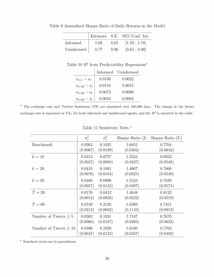
Table 9 Annualized Sharpe Ratio of Daily Returns in the Model

Estimate S.E. 95% Conf. Int.

Informed 1.68 0.05 [1.59 , 1.78]

Uninformed 0.77 0.06 [0.64 , 0.90]

Table 10 R2 from Predictability Regressions∗

Informed Uninformed

st+1 − st 0.0130 0.0022

st+20 − st 0.0144 0.0015

st+40 − st 0.0073 0.0006

st+60 − st 0.0042 0.0003

∗ The exchange rate and Twitter Sentiment (TS) are simulated over 100,000 days. The change in the future

exchange rate is regressed on TSt, for both informed and uninformed agents, and the R2 is reported in the table.

Table 11 Sensitivity Tests ∗

σIv σU

v Sharpe Ratio (I) Sharpe Ratio (U)

Benchmark 0.0362 0.1031 1.6852 0.7704

(0.0067) (0.0189) (0.0502) (0.0642)

k = 10 0.0313 0.0757 1.3524 0.6952

(0.0037) (0.0088) (0.0437) (0.0548)

k = 20 0.0410 0.1001 1.4867 0.7666

(0.0076) (0.0184) (0.0525) (0.0549)

k = 30 0.0400 0.0996 1.5543 0.7839

(0.0057) (0.0142) (0.0497) (0.0574)

T = 20 0.0176 0.0412 1.4648 0.8122

(0.0012) (0.0028) (0.0522) (0.0519)

T = 60 0.0740 0.2120 1.6269 0.7451

(0.0212) (0.0602) (0.1116) (0.0913)

Number of Tweets ≥ 5 0.0362 0.1031 1.7187 0.7670

(0.0066) (0.0187) (0.0493) (0.0632)

Number of Tweets ≥ 10 0.0396 0.1029 1.6180 0.7702

(0.0047) (0.0123) (0.0427) (0.0482)

∗ Standard errors are in parentheses.

50

Appendix A

Tables A1 and A2 show all word combinations used to categorize tweets as positive,

negative and neutral. Table A1 lists the word combinations in each category that require

the explicit absence of some other words. Table A2 shows the list of word combinations

whose existence in a tweet is enough to place the tweet in one of the categories.

“*” and “?” are wildcard characters. “*” represents one or more characters and “?” rep-

resents one character. For instance, “*buy??eur*” is a match with any tweet that contains

the words “buy” and “eur” in this order and with exactly two characters between them.

“*” before “buy” and after “eur” means that there could be any number of characters in a

tweet before “buy” or after “eur”. This word combination is intended to identify positive

tweets that contain expressions such as “buy $eurusd” or “buy #euro”. In both cases, all

the criteria of a match with “*buy??eur*” are satisfied. There are exactly two characters

between “buy” and “eur”. In the case of “buy $eurusd”, there are three characters after

“eur” and in “buy #euro” there is only one character after “eur”. Both are acceptable re-

placements for the wildcard character “*”. In both examples, there is no character before

“buy”. Since “*” could be replaced with zero or any number of characters, no character

before “buy” is considered a match with “*buy??eur*”.

51

Table A1: Word combinations used to identify opinionated tweets.

Positive

Include ... and not include ...

”*buy??eur*” or ”*close*buy*eur*” , ”*exit*buy*eur*”,

”*buy?eur*” ”*close*buy?eurusd*”, ”*close*buy?eurusd*”,

”*close*buy??eur\usd*”, ”*buy*,*eur*”, ”*buy*:*eur*”,

”*buy*fade*”, ”*close*buy??eur\usd*”

”*never*buy*eur*”

”*buy*lot*eur*” ”*close*buy*lot*eur*”

”*long??eur*” ”*long?term*”, ”*was?long*”, ”*close*long??eur*”,

”*close*long?eur*”, ”*exit*long??eur*”, ”*exit*long?eur*”

”*bullish*” ”*absent*”, ”*absence*”, ”*void*”, ”*lack*”,

”*bullish*fail*”, ”*fail*bullish*”, ”*bullish*invalid*”,

”*bullish*break*”, ”*nothing*bullish*”, ”*missing*”,

”*were?bullish*”, ”*was?bullish*”, ”*no?bullish*”,

”*not?bullish*”, ”*market is bullish*”

”*covered*short*” ”*short?term*”

”*buy?the?eur*” ”*never?buy?the?eur*”, ”*not?buy?the?eur*”

”*eur?usd*look?good*” ”*eur?usd*not*look?good*”

”*eur?usd*looks?good*” ”*eur?usd*not*looks?good*”

”*double*long*” ”*long?term*”

”*took*long*position*” ”*long?term*”

”*out*of*eur*short*” ”*short?term*” , ”*stop*out*of*eur*short*”

”*add*eur*long*” ”*long?term*” , ”*addict*” , ”*dadd*”

52

Table A1 (Continued): Word combinations used to identify opinionated tweets.

Positive

Include ... and not include ...

”*increase*eur*long*” ”*long?term*” , ”*long?off*”

”*up*accelerate*trend*” ”*update*”

”*signals?buy*eur*” ”*forexsignals*”

”*long?signal*” ”*long?term*” , ”*wait*for*long?signal*”

”*higher?high*” ”*if*higher?high*”

”*take*eur?usd*long*” ”*took*profit*”

”*took*eur?usd*long*” ”*took*profit*” , ”*took*opportunity*”

”*further*buying*” ”*buying*usd*”

”*further*eur*gain*” ”*against*”

”*dip*buy*” or ”*dip*;*eurusd*”, ”*dip*;*eur?usd*”,

”*buy*dip*” ”*buy*dips?in?cable*”, ”*buy*dip?in?cable*”

”*sell*rall*”

”*look*to*buy*” ”*looks?like*” , ”*look*to*buy*put*”

”*buying?the?eur*” ”*buying?the?eur*was*”,

”*about*buying?the?eur*”,

”*buying?the?eur*tomorrow*”

”*trigger*further*eurusd*gain*” or ”*against*”

”*trigger*further*eur?usd*gain*”

”*offer*long*entr*” ”*long?term*”

”*look*to*long*” ”*long?term*” , ”*looks*”

”*eur?usd*may*extend*gain*” or ”*against*”

”*eurusd*may*extend*gain*” or

”*eur?usd*will*extend*gain*” or

”*eurusd*will*extend*gain*” or

”*eur?usd*set*extend*gain*” or

”*eurusd*set*extend*gain*”

”eurusd*targets?higher*” or ”*higher?low*”

”*eur?usd*target?higher*”

53

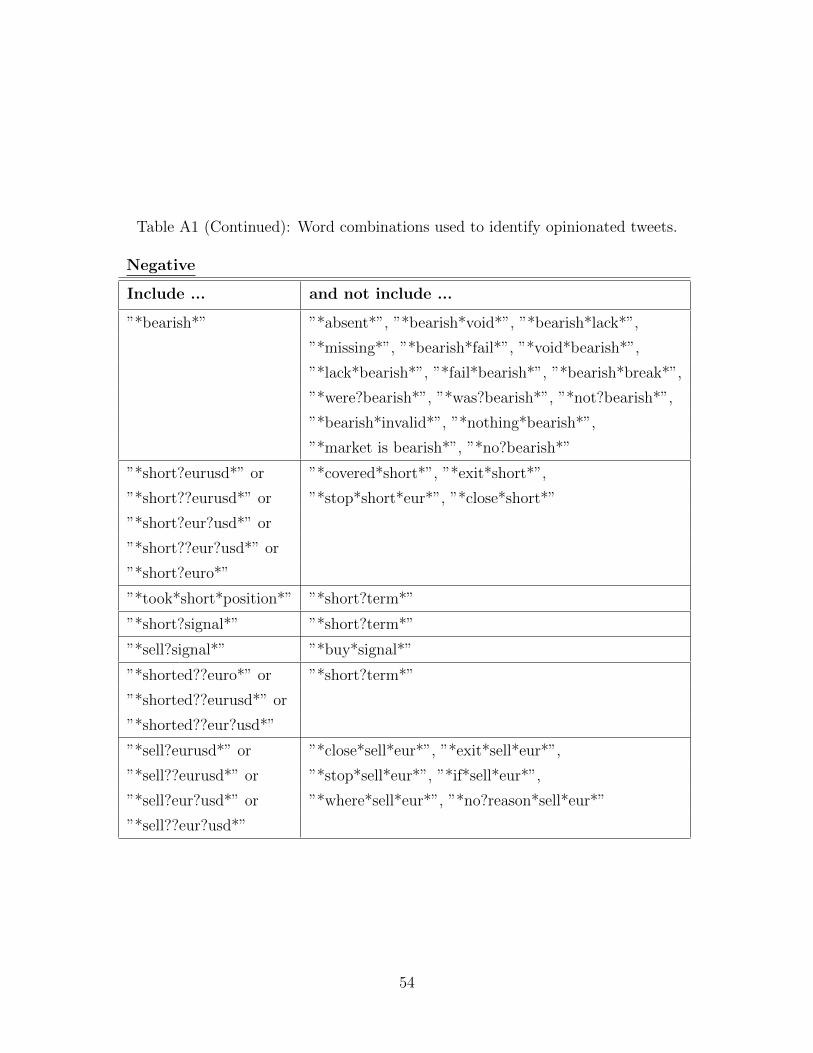
Table A1 (Continued): Word combinations used to identify opinionated tweets.

Negative

Include ... and not include ...

”*bearish*” ”*absent*”, ”*bearish*void*”, ”*bearish*lack*”,

”*missing*”, ”*bearish*fail*”, ”*void*bearish*”,

”*lack*bearish*”, ”*fail*bearish*”, ”*bearish*break*”,

”*were?bearish*”, ”*was?bearish*”, ”*not?bearish*”,

”*bearish*invalid*”, ”*nothing*bearish*”,

”*market is bearish*”, ”*no?bearish*”

”*short?eurusd*” or ”*covered*short*”, ”*exit*short*”,

”*short??eurusd*” or ”*stop*short*eur*”, ”*close*short*”

”*short?eur?usd*” or

”*short??eur?usd*” or

”*short?euro*”

”*took*short*position*” ”*short?term*”

”*short?signal*” ”*short?term*”

”*sell?signal*” ”*buy*signal*”

”*shorted??euro*” or ”*short?term*”

”*shorted??eurusd*” or

”*shorted??eur?usd*”

”*sell?eurusd*” or ”*close*sell*eur*”, ”*exit*sell*eur*”,

”*sell??eurusd*” or ”*stop*sell*eur*”, ”*if*sell*eur*”,

”*sell?eur?usd*” or ”*where*sell*eur*”, ”*no?reason*sell*eur*”

”*sell??eur?usd*”

54

Table A1 (Continued): Word combinations used to identify opinionated tweets.

Negative

Include ... and not include ...

”*sell the eur*” ”*where*sell the eur*”

”*short the eur*” ”*was*short the eur*”

”*add*eur*short*” ”*short?term*” , ”*addict*”

, ”*dadd*”

”*sold*rally*” ”*oversold*”

”*sold*bounce*” ”*oversold*bounce*”

”*eurusd*toppy*” or ”*stopp*” , ”*dollar?topp*”

”*eurusd*topping*” or , ”*audusd??topp*”

”*eur?usd*toppy*” or

”*eur?usd*topping*”

”*bounce*sold*” ”*oversold*”

”*good?short*” ”*short?term*”

”*take*eur*short*” ”*take*profit*eur*short*”, ”*take*out*eur*short*”,

”*take*rest*eur*short*”

”*took*eur*short*” ”*took*profit*eur*short*”, ”*took*out*eur*short*”,

”*took*rest*eur*short*”

”*further*loss*” ”*dollar*further*loss*”

”*further?fall*” ”*dollar*further?fall*”

”*next*leg*lower*” ”*long?term*”

Neutral

”*watch*” ”*video*”, ”*marketwatch*”,

”*watchlist*”, ”*iwatch*”

”*out*eur*long*” ”*break*out*”

55

Table A2: Word combinations used to identify opinionated tweets.

Positive

”*buy??fxe*” ”*long??fxe*” ”*buy?signal*”

”*upside*breakout*” ”*eur?usd*bull*intact*” ”*expect*move*higher*”

”*oversold*eur*” ”*eur?usd*oversold*” ”*ascending*triangle*”

”*increase*bullish*bet*” ”*bought*rebound*” ”*will*move*higher*today*”

”*bought*dip*” ”*bought*bounce*” ”*will*higher*today*”

”*should?buy*dip*” ”*rally*has*leg*” ”*buy*above*moving*average*”

”*tradable*bottom*” ”*eur?usd*good?buy*” ”*raise*eur*exposure*”

”*will*see*higher*” or ”*eur?usd*bias*upside*” or ”*eur?usd?will?rise*” or

”*going?to*see*higher*” ”*eur?usd*bias*positive*” ”*eur?usd?will?continue?to?rise*”

”*euro?bottoming*” or ”*staying?long?eur?usd*” or ”*eur?usd*heads*higher*” or

”*eur?usd?bottoming*” ”*staying?long??eur?usd*” ”*eur?usd*heading*higher*”

”*bottom?is?in*” ”*oversold*bounce*” ”*sticking*with*long*”

”*potential?buy*” ”*resume*bull*trend*” ”*dollar*further*loss*”

”*long?favor*” ”*suggest*bull*control*” ”*suggest*advance*continue*”

”*spark*eur*buy*” or ”*eurusd?could?bottom*” or ”*further*rise*ahead*” or

”*initiat*eur*buy*” ”*euro?could?bottom*” ”*further*advance*ahead*”

”*stay??eurusd?long*” or ”*currently?long??eurusd*” or ”*increase*eurusd?long*”

”*stay?eurusd?long*” or ”*currently?long?eurusd*” or ”*increase*long?eurusd*”

”*stay??eur?usd?long*” or ”*currently?long??eur?usd*” or ”*increase*eur\usd?long*”

”*stay?eur?usd?long*” ”*currently?long?eur?usd*” ”*increase*long?eur\usd*”

”*increase*eurusd?long*” ,

”*decrease*eurusd?long*” ,

”*hold*eurusd?long*” ,

”*keep*eurusd?long*” ,

”*increase*eur?usd?long*” ,

”*decrease*eur?usd?long*” ,

”*hold*eur?usd?long*” ,

”*keep*eur?usd?long*”

56

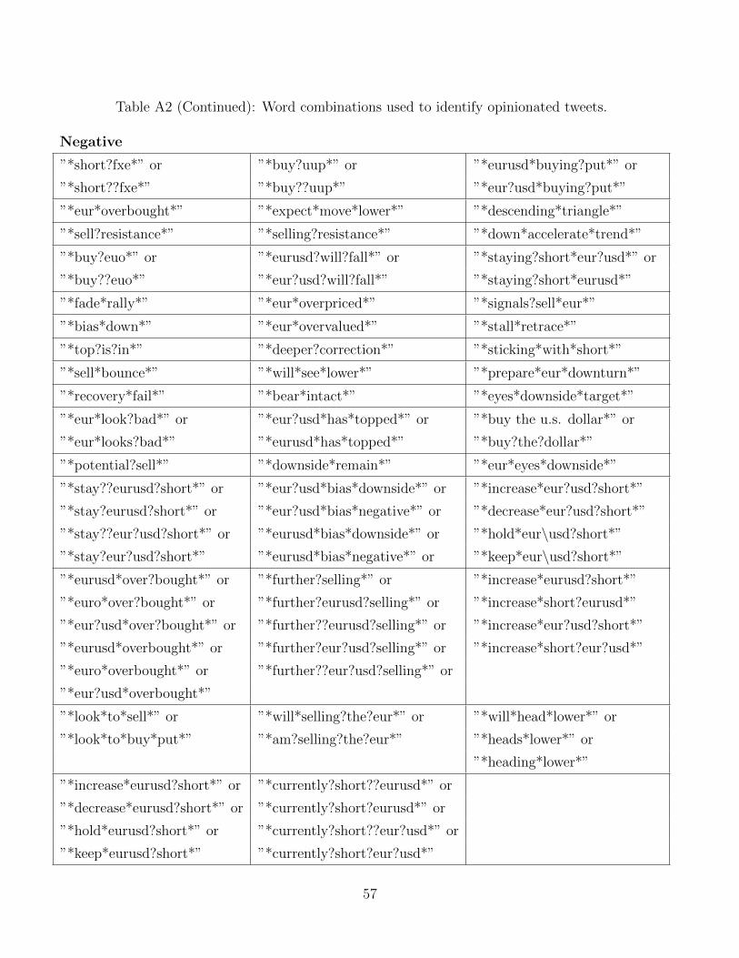
Table A2 (Continued): Word combinations used to identify opinionated tweets.

Negative

”*short?fxe*” or ”*buy?uup*” or ”*eurusd*buying?put*” or

”*short??fxe*” ”*buy??uup*” ”*eur?usd*buying?put*”

”*eur*overbought*” ”*expect*move*lower*” ”*descending*triangle*”

”*sell?resistance*” ”*selling?resistance*” ”*down*accelerate*trend*”

”*buy?euo*” or ”*eurusd?will?fall*” or ”*staying?short*eur?usd*” or

”*buy??euo*” ”*eur?usd?will?fall*” ”*staying?short*eurusd*”

”*fade*rally*” ”*eur*overpriced*” ”*signals?sell*eur*”

”*bias*down*” ”*eur*overvalued*” ”*stall*retrace*”

”*top?is?in*” ”*deeper?correction*” ”*sticking*with*short*”

”*sell*bounce*” ”*will*see*lower*” ”*prepare*eur*downturn*”

”*recovery*fail*” ”*bear*intact*” ”*eyes*downside*target*”

”*eur*look?bad*” or ”*eur?usd*has*topped*” or ”*buy the u.s. dollar*” or

”*eur*looks?bad*” ”*eurusd*has*topped*” ”*buy?the?dollar*”

”*potential?sell*” ”*downside*remain*” ”*eur*eyes*downside*”

”*stay??eurusd?short*” or ”*eur?usd*bias*downside*” or ”*increase*eur?usd?short*”

”*stay?eurusd?short*” or ”*eur?usd*bias*negative*” or ”*decrease*eur?usd?short*”

”*stay??eur?usd?short*” or ”*eurusd*bias*downside*” or ”*hold*eur\usd?short*”

”*stay?eur?usd?short*” ”*eurusd*bias*negative*” or ”*keep*eur\usd?short*”

”*eurusd*over?bought*” or ”*further?selling*” or ”*increase*eurusd?short*”

”*euro*over?bought*” or ”*further?eurusd?selling*” or ”*increase*short?eurusd*”

”*eur?usd*over?bought*” or ”*further??eurusd?selling*” or ”*increase*eur?usd?short*”

”*eurusd*overbought*” or ”*further?eur?usd?selling*” or ”*increase*short?eur?usd*”

”*euro*overbought*” or ”*further??eur?usd?selling*” or

”*eur?usd*overbought*”

”*look*to*sell*” or ”*will*selling?the?eur*” or ”*will*head*lower*” or

”*look*to*buy*put*” ”*am?selling?the?eur*” ”*heads*lower*” or

”*heading*lower*”

”*increase*eurusd?short*” or ”*currently?short??eurusd*” or

”*decrease*eurusd?short*” or ”*currently?short?eurusd*” or

”*hold*eurusd?short*” or ”*currently?short??eur?usd*” or

”*keep*eurusd?short*” ”*currently?short?eur?usd*”

57

Table A2 (Continued): Word combinations used to identify opinionated tweets.

Neutral

”*were?bearish*” or ”*no?bearish*” or ”*not*expect*move*higher*” or

”*were?bullish*” or ”*no?bullish*” or ”*not*expect*move*lower*”

”*was?bearish*” or ”*not?bearish*” or

”*was?bullish*” ”*not?bullish*”

”*bullish*absent*” or ”*bullish*lack*” or ”*bullish*missing*” or

”*bearish*absent*” or ”*lack*bullish*” or ”*missing*bullish*” or

”*bullish*void*” or ”*bearish*lack*” or ”*bearish*missing*” or

”*bearish*void*” ”*lack*bearish*” ”*missing*bearish*”

”*bought*sold*” or ”*will*buy*if*” or ”*might*buy*eur*”

”*sold*bought*” ”*will*sell*if*” ”*might*sell*eur*”

”*could?go?higher*” or ”*needs?confirm*” or ”*bullish*fail*” or

”*could?go?lower*” or ”*need?to?see*” or ”*fail*bullish*” or

”*could?move?higher*” or ”*needs?to?hold*” or ”*bearish*fail*” or

”*could?move?lower*” ”*need?to?hold*” ”*fail*bearish*”

”*must?close*” or ”*buy*signal*watch*” or ”*bullish*decline*” or

”*should?close*” ”*sell*signal*watch*” ”*bullishness*decrease*”

”*bull*lose*steam*” or ”*neutral?on??eur*” or ”*eur*need*go*lower*” or

”*bear*lose*steam*” ”*neutral?on?eur*” ”*eur*need*go*higher*”

”*wait*” ”*not*trading*” ”*staying?in?cash*”

”*rally*weak*” ”*patience*” ”*no?need*do?anything*”

”*not?yet*” ”*looking?for*” ”*not?doing?much*”

”*staying?flat*” ”*bounce?possible*” ”*will?be?telling*”

”*all?eyes*on*” ”*steady*ahead*” ”*could*accelerate*”

”*bull*doubt*” or ”*no*new*trade*” ”*out*eur*short*” or

”*bear*doubt*” ”*out*eur*long*”

”*no?trend*” ”*range?in?focus*” ”*may*hold*range*”

”*indecision*” ”*look?to?see*” ”*bias*remain*neutral*”

”*hesitation*”

58