What can we do with a mesoscale meteorological model ? Focus on forecasting of heavy precipitation events by Franck Lascaux Keywords: Meso-NH, high resolution,

What can we do with a What can we do with a mesoscale meteorological mesoscale meteorological

model ? model ? Focus on forecasting of heavy Focus on forecasting of heavy

precipitation eventsprecipitation events

by

Franck Lascaux

Keywords: Meso-NH, high resolution, heavy precipitation

Picture of a developing storm

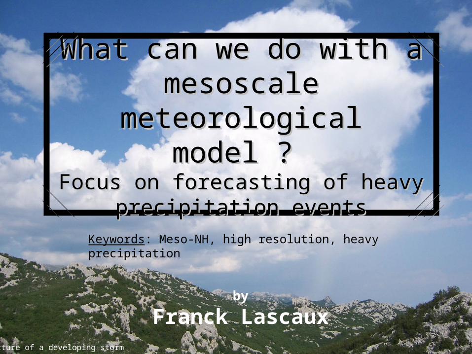
My previous work during my PhD

Use of the Meso-NH meteorological model (developed jointly by CNRM at Météo-France and Laboratoire d’Aérologie, Toulouse).

1 – A detailed numerical study of a highly convective event.

2 – Mesoscale data assimilation at fine scale.

3 – Compared microphysical study of three different heavy precipitation events.

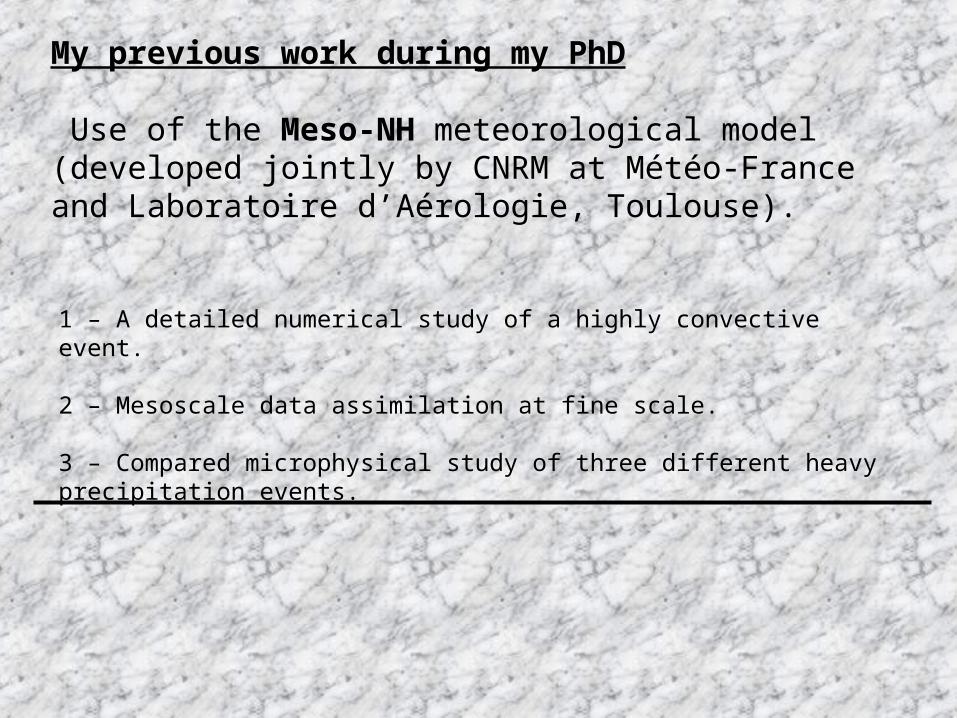
Adapted from Anthes et al., 1975 – Time and space scales of atmospheric motions

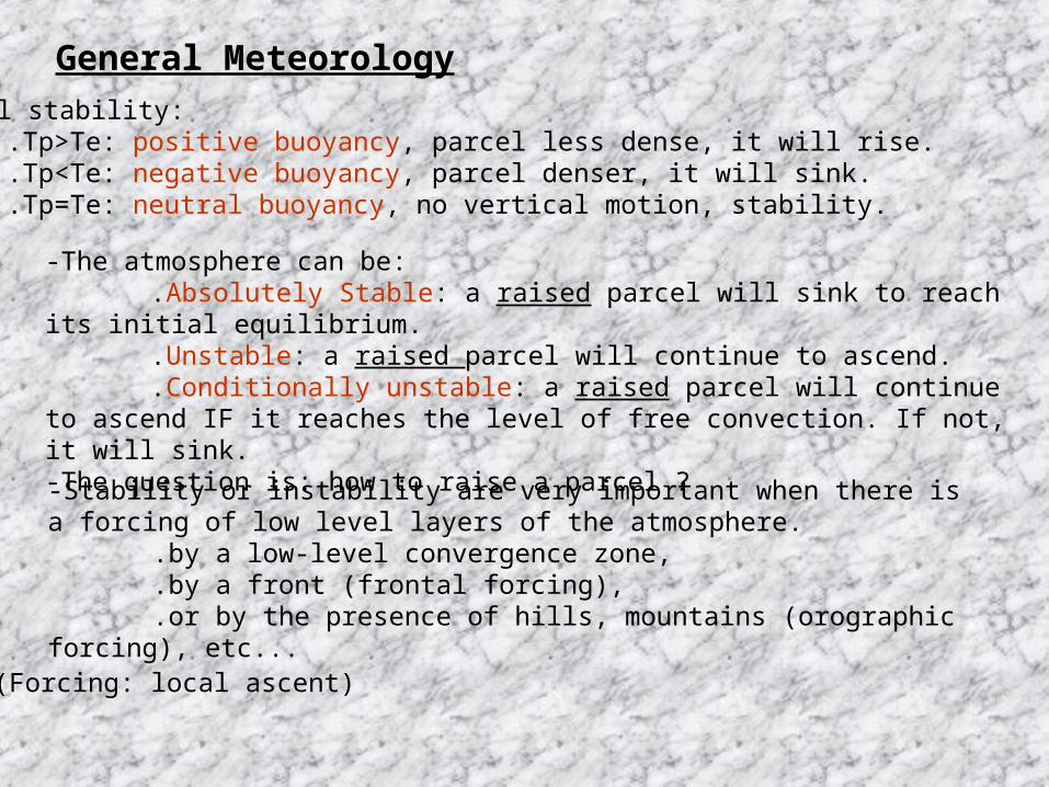
General Meteorology-Parcel stability:

.Tp>Te: positive buoyancy, parcel less dense, it will rise.

.Tp<Te: negative buoyancy, parcel denser, it will sink.

.Tp=Te: neutral buoyancy, no vertical motion, stability.

-The atmosphere can be:.Absolutely Stable: a raised parcel will sink to reach its initial equilibrium..Unstable: a raised parcel will continue to ascend..Conditionally unstable: a raised parcel will continue to ascend IF it

reaches the level of free convection. If not, it will sink.-The question is: how to raise a parcel ?

-Stability or instability are very important when there is a forcing of low level layers of the atmosphere.

.by a low-level convergence zone,

.by a front (frontal forcing),

.or by the presence of hills, mountains (orographic forcing), etc...

(Forcing: local ascent)

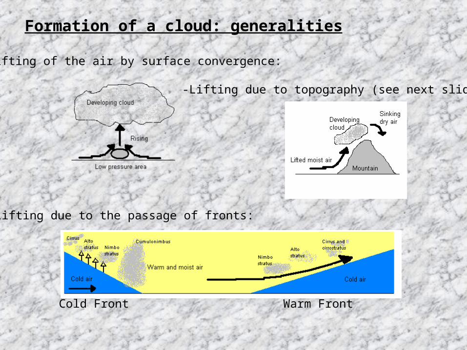
Formation of a cloud: generalities

-Lifting of the air by surface convergence:

-Lifting due to topography (see next slide):

-Lifting due to the passage of fronts:

Cold Front Warm Front

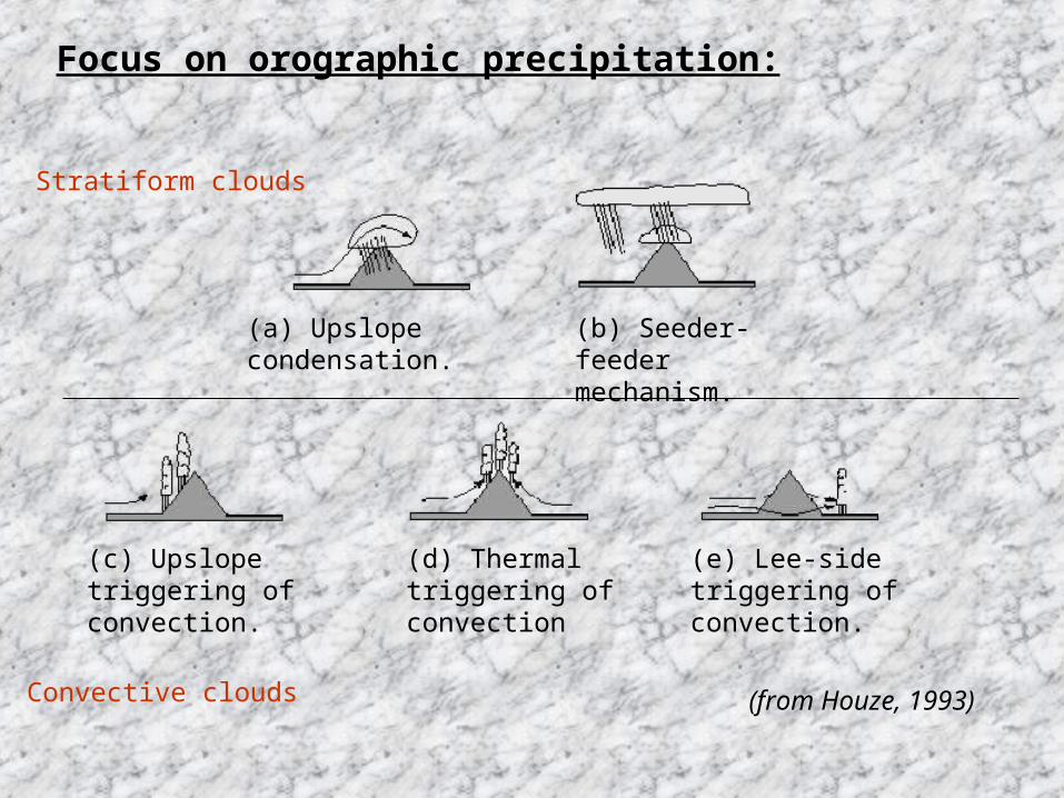
Focus on orographic precipitation:

(b) Seeder-feeder mechanism.

(a) Upslope condensation.

(c) Upslope triggering of convection.

(d) Thermal triggering of convection

(e) Lee-side triggering of convection.

(from Houze, 1993)

Stratiform clouds

Convective clouds

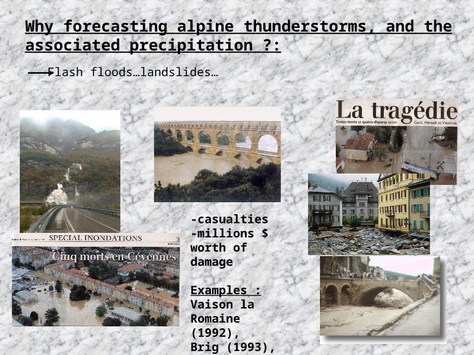
Why forecasting alpine thunderstorms, and the associated precipitation ?:

-casualties-millions $ worth of damage

Examples : Vaison la Romaine (1992),Brig (1993), Cévennes Mountains (2002).

Flash floods…landslides…

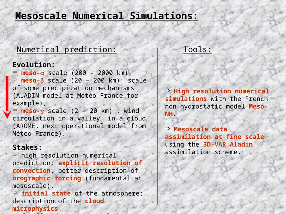
Numerical prediction:

Evolution: mesoscale (200 – 2000 km), mesoscale (20 – 200 km): scale of some precipitation mechanisms (ALADIN model at Météo-France for example), mesoscale (2 – 20 km) : wind circulation in a valley, in a cloud (AROME, next operational model from Météo-France).

Stakes: high resolution numerical prediction: explicit resolution of convection, better description of orographic forcing (fundamental at mesoscale). initial state of the atmosphere; description of the cloud microphysics. finally, improvement of the prediction of mesocale phenomena (squall lines, storms…) and the associated precipitation.

Tools:

High resolution numerical simulations with the French non hydrostatic model Meso-NH.

Mesoscale data assimilation at fine scale using the 3D-VAR Aladin assimilation scheme.

Mesoscale Numerical Simulations:

Hail

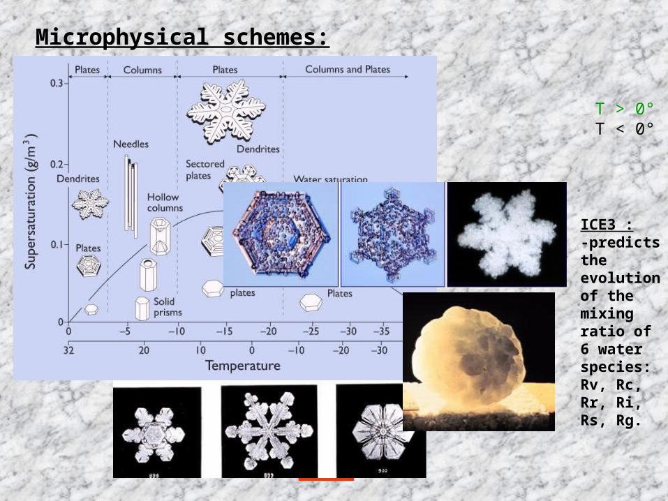
T > 0°T < 0°

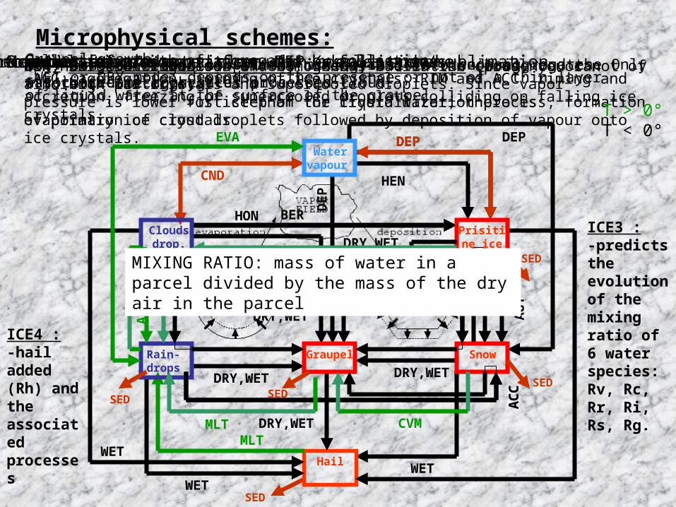
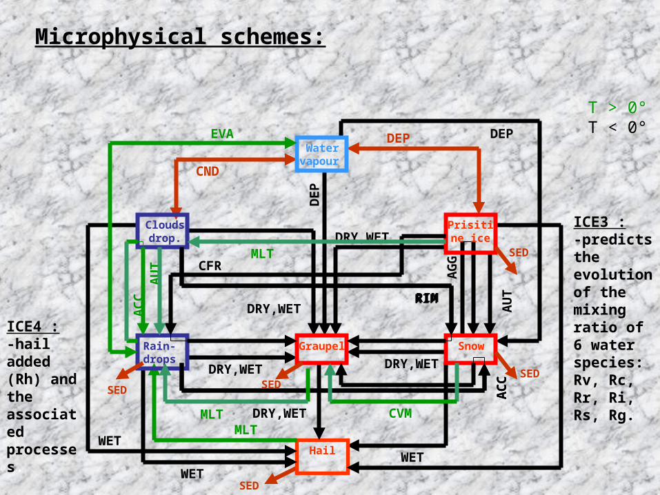
ICE3 :-predicts the evolution of the mixing ratio of 6 water species: Rv, Rc, Rr, Ri, Rs, Rg.

Water vapou

r

Clouds drop.

Prisitine ice

Rain- drops

SnowGraupel

Microphysical schemes:

BER

DEP

BER: Bergeron-Findeisen effect. When T<0°C in the cloud, you can find both ice crystals and supercooled droplets. Since vapor pressure is lower for ice than for liquid water, there is evaporation of cloud droplets followed by deposition of vapour onto ice crystals.

AU

T

AUT: autoconversion of primary ice crystal into snow aggregates. Only way to create aggregates in a cold cloud.

DRY,WET DRY,WET

DRY,WET

DRY,WETD

EP

Graupel growth:-WET or DRY mode: depends on the presence or not of a thin layer of liquid water at the surface of the graupel.

SED

Hail WET

MLTWET

WET

ICE4 :-hail added (Rh) and the associated processes.

DRY,WET

ICE4 scheme: Prediction of the mixing ratio of the hail, and the associated microphysical processes.

DEP

AG

G

RIM

AC

C

Collection growth of aggregates by collection:-AGG: aggregation, joining of ice crystals; RIM and ACC: riming and accretion, freezing of supercooled droplets colliding on falling ice crystals.

HON

HEN

HEN,HON: -heterogeneous and homogenous nucleation (presence or not of a foreign particle). -1st step of the crystallization process, formation of primary ice crystals.

CND

DEP

CND: condensation/evaporation; DEP: deposition/sublimation

T > 0°T < 0°


Water vapou

r

Clouds drop.

Prisitine ice

Rain- drops

SnowGraupel


CFR

AC

C

RIM

Graupel formation

MLT

CVMMLT

Melting process

AU

TA

CC

EVA

Warm processes, adapted from the Kessler scheme.

SED SEDSED

SED

Sedimentation of the particles with a fall speed.

MIXING RATIO: mass of water in a parcel divided by the mass of the dry air in the parcel

AU

T

DRY,WET DRY,WET

DRY,WET

DRY,WETD

EP

SED

Hail WET

MLTWET

WET

ICE4 :-hail added (Rh) and the associated processes.

DRY,WET

DEP

AG

G

RIM

AC

C

CND

DEP

T > 0°T < 0°


Water vapou

r

Clouds drop.

Prisitine ice

Rain- drops

SnowGraupel


CFR

AC

C

RIM

MLT

CVMMLT

AU

TA

CC

EVA

SED SEDSED

SED

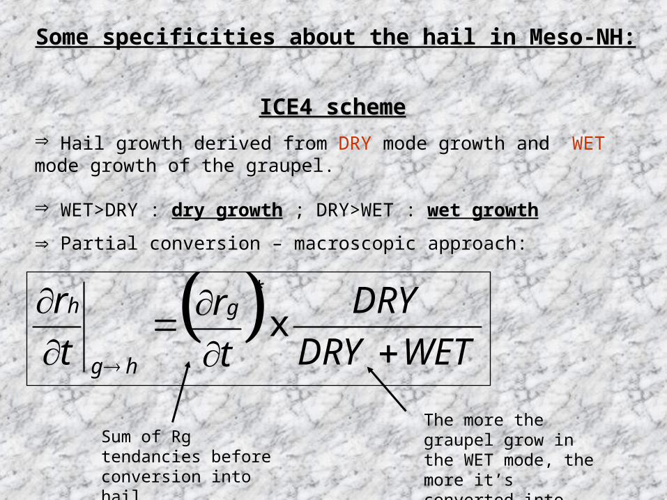
Hail growth derived from DRY mode growth and WET mode growth of the graupel.

WET>DRY : dry growth ; DRY>WET : wet growth

Partial conversion – macroscopic approach:

WETDRY

DRY

t

rt

r g

hg

h

x*

Sum of Rg tendancies before conversion into hail.

The more the graupel grow in the WET mode, the more it’s converted into hail.

ICE4 schemeICE4 scheme

Some specificities about the hail in Meso-NH:

Numerical simulations of different precipitation events:

.In Autumn 1999 a campaign took place over the Alps to collect large amount of data : it’s the MAP (Mesoscale Alpine Programme) campaign.

.Different heavy precipitation events were observed above the Lago Maggiore Area.

.The data collected were used to validate simulations ran with Meso-NH, with a focus on sensitivity to the microphysical scheme used, sensitivity to the initial conditions, and the possibility of discriminate between events with different incoming flow characteristics.

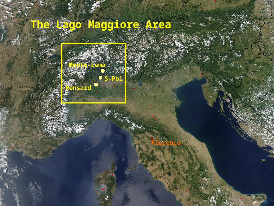
The Lago Maggiore Area

S-Pol

Ronsard

Monte-Lema

Florence

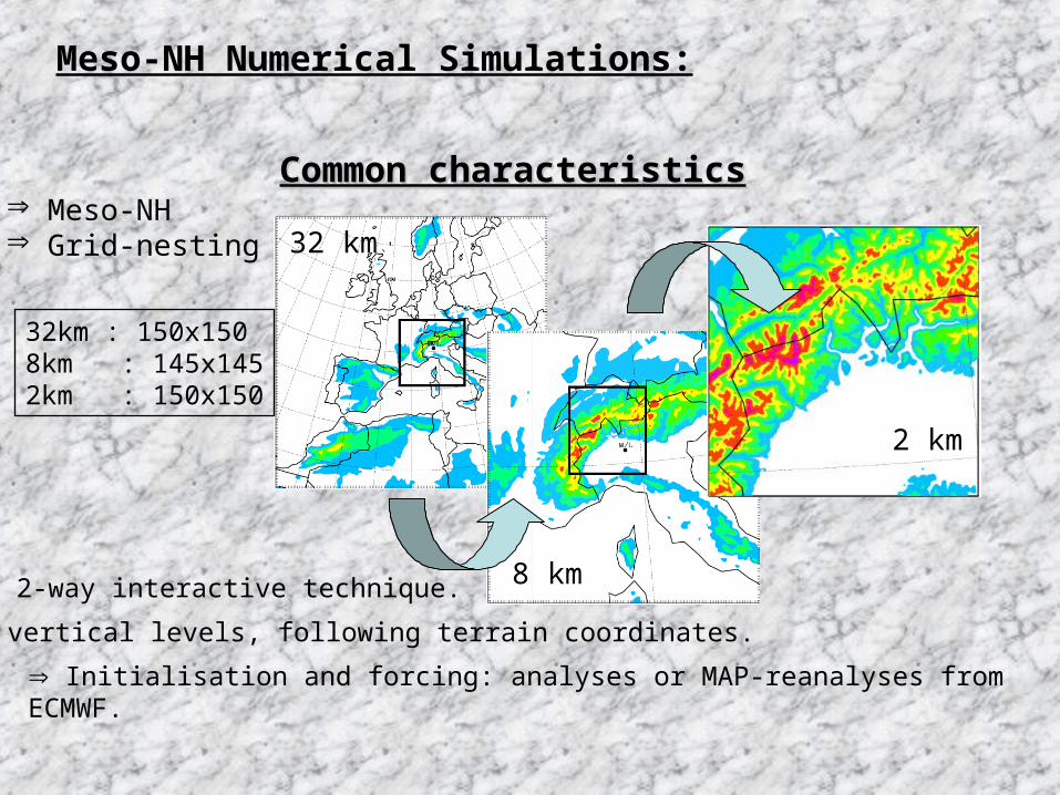
Common characteristicsCommon characteristics

32 km

8 km

2 km

2-way interactive technique.

51 vertical levels, following terrain coordinates.

Initialisation and forcing: analyses or MAP-reanalyses from ECMWF.

Meso-NH Grid-nesting

32km : 150x1508km : 145x1452km : 150x150

Meso-NH Numerical Simulations:

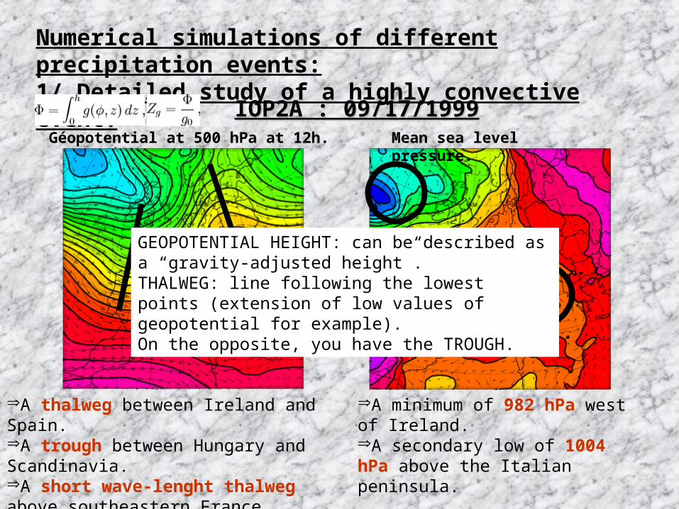
IOP2A : 09/17/1999IOP2A : 09/17/1999Géopotential at 500 hPa at 12h. Mean sea level

pressure.

A minimum of 982 hPa west of Ireland.A secondary low of 1004 hPa above the Italian peninsula.

A thalweg between Ireland and Spain.A trough between Hungary and Scandinavia.A short wave-lenght thalweg above southeastern France.

Numerical simulations of different precipitation events:1/ Detailed study of a highly convective event.

GEOPOTENTIAL HEIGHT: can be described as a “gravity-adjusted height”. THALWEG: line following the lowest points (extension of low values of geopotential for example).On the opposite, you have the TROUGH.

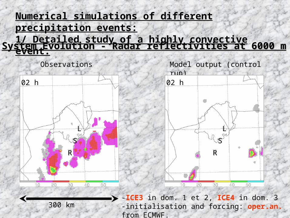
System Evolution - Radar reflectivities at 6000 mSystem Evolution - Radar reflectivities at 6000 m

Observations Model output (control run)

300 km

18h 18h19 h19 h20 h 20 h21 h 21 h22 h 22 h23 h23 h00 h 00 h01 h01 h02 h 02 h

R

S

L

R

S

L

-ICE3 in dom. 1 et 2, ICE4 in dom. 3-initialisation and forcing: oper.an. from ECMWF.


Good temporal phasing between observed and modelled systems. Good spatial localisation of the reflectivity maxima in the higher levels (where only hailstones can produce such maxima).

However, under-estimation of the horizontal extent of lower reflectivities.

Conclusions on the development of the system :


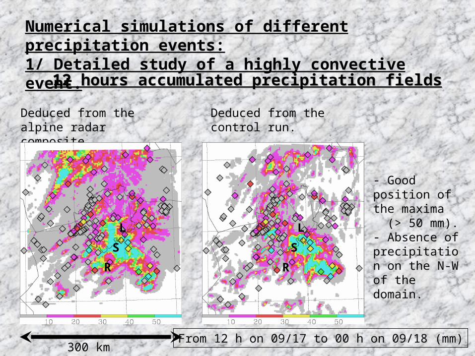
Deduced from the alpine radar composite.

Deduced from the control run.

12 hours accumulated precipitation fields12 hours accumulated precipitation fields

From 12 h on 09/17 to 00 h on 09/18 (mm)

R

S

L

R

S

L

- Good position of the maxima (> 50 mm).- Absence of precipitation on the N-W of the domain.

300 km


Meso-NH model succeeds well in reproducing the convective system of the MAP-IOP2A, and the associated precipitation fields.

Good job !

However, can we improve the results ? idea: using the MAP-reanalyses dataset from the ECMWF. A new set of reanalysis with additional data included.


FIRST CONCLUSIONS

You know what ?I’m happy.

R

S

L

300 km

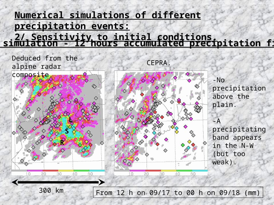
Deduced from the alpine radar composite. CEPRA.

New simulation - 12 hours accumulated precipitation fieldsNew simulation - 12 hours accumulated precipitation fields

From 12 h on 09/17 to 00 h on 09/18 (mm)

-No precipitation above the plain.

-A precipitating band appears in the N-W (but too weak).

Numerical simulations of different precipitation events:2/ Sensitivity to initial conditions.

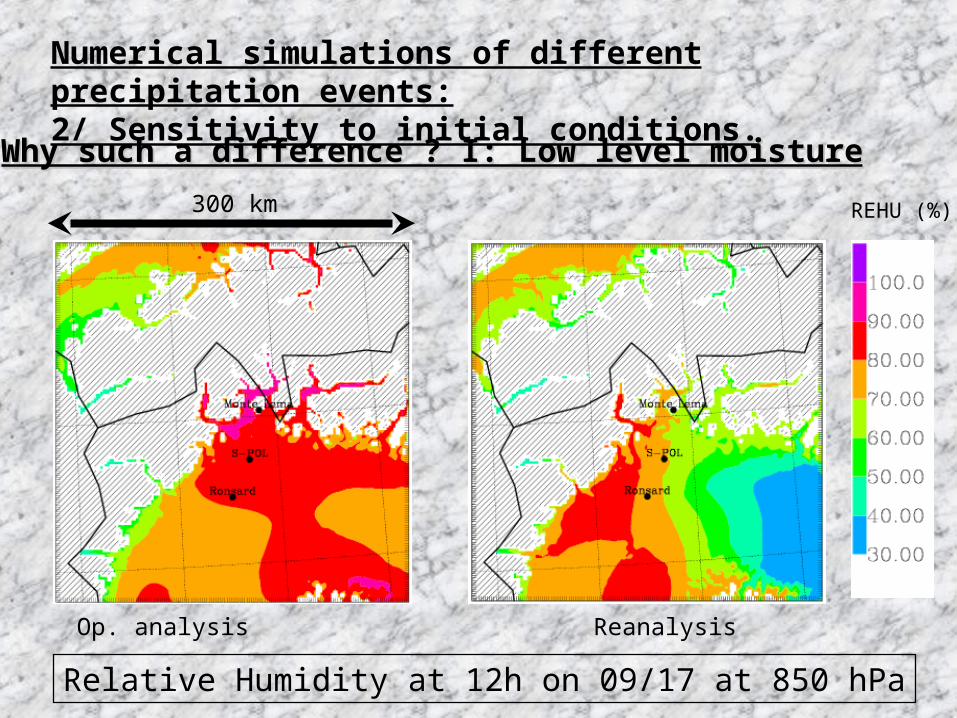
REHU (%)

Relative Humidity at 12h on 09/17 at 850 hPa

Why such a difference ? I: Low level moistureWhy such a difference ? I: Low level moisture

300 km

Op. analysis Reanalysis


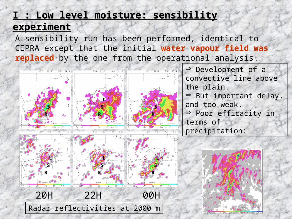
I : Low level moisture: sensibility experimentI : Low level moisture: sensibility experiment

20H 22H 00H

A sensibility run has been performed, identical to CEPRA except that the initial water vapour field was replaced by the one from the operational analysis.

Radar reflectivities at 2000 m

Development of a convective line above the plain. But important delay, and too weak. Poor efficacity in terms of precipitation:

R

S

L

R

S

L

R

S

L

R

S

L

R

S

L

R

S

L

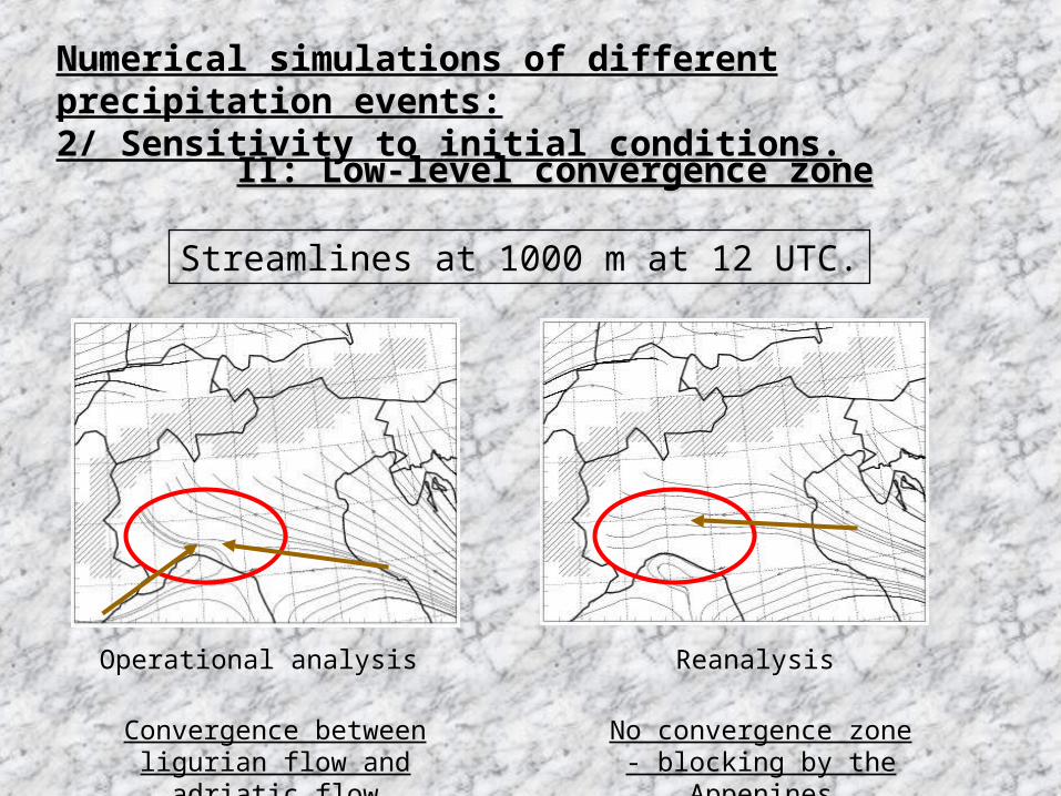
Streamlines at 1000 m at 12 UTC.

II: Low-level convergence zoneII: Low-level convergence zone

Operational analysis Reanalysis

Convergence between ligurian flow and adriatic

flow

No convergence zone - blocking by the

Appenines


The MAP-IOP2a exhibits a stong sensibility to the initial conditions.

Some differences between op. an. and rean. may explain these discrepancies between the simulations:- a atmosphere drier in the lower levels.- a blocking of the ligurian flow by the Appenines more important leading to a less pronounced convergence zone.

Low predictability of this event.

Numerical simulations of different precipitation events:2/ Sensitivity to initial conditions. CONCLUSIONS.

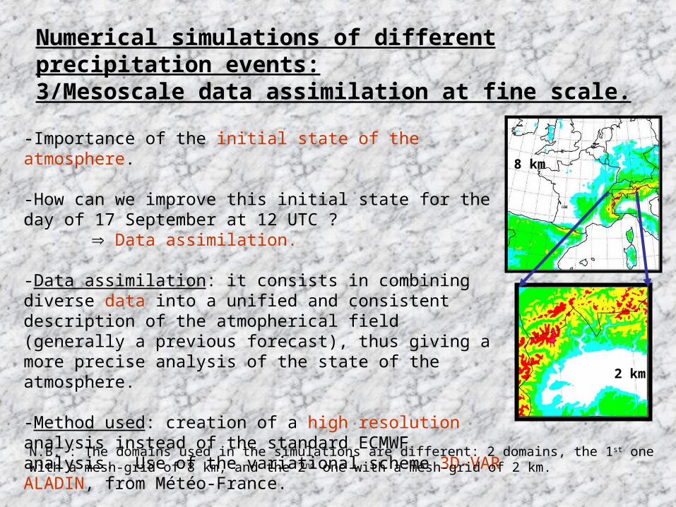
-Importance of the initial state of the atmosphere.

-How can we improve this initial state for the day of 17 September at 12 UTC ?

Data assimilation.

-Data assimilation: it consists in combining diverse data into a unified and consistent description of the atmopherical field (generally a previous forecast), thus giving a more precise analysis of the state of the atmosphere.

-Method used: creation of a high resolution analysis instead of the standard ECMWF analysis. Use of the variational scheme 3D-VAR ALADIN, from Météo-France. N.B. : The domains used in the simulations are different: 2 domains, the 1st one with a mesh-grid of 8 km, and the 2nd one with a mesh-grid of 2 km.

8 km

2 km

Numerical simulations of different precipitation events:3/Mesoscale data assimilation at fine scale.

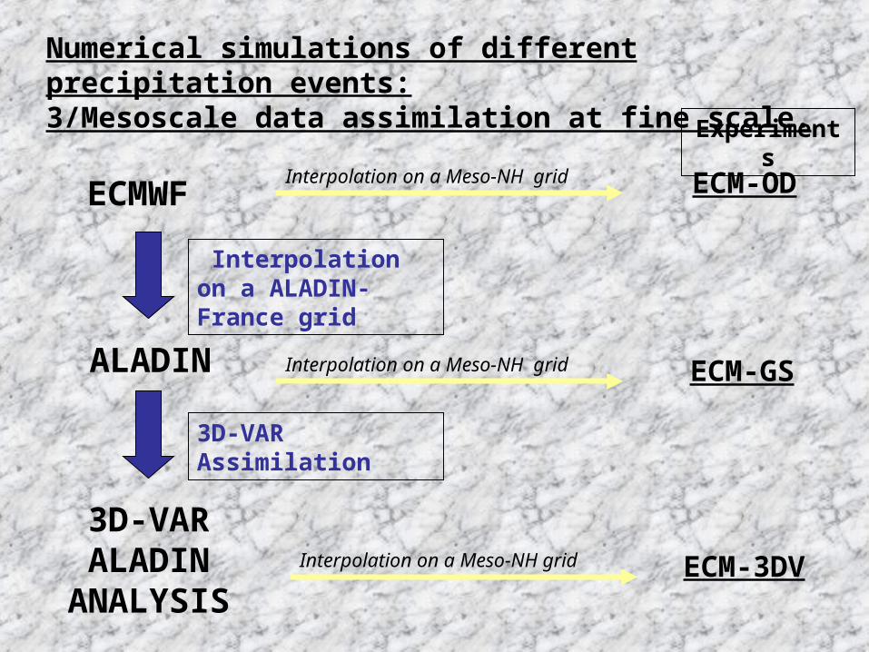
ECMWF

ALADIN

3D-VARALADIN

ANALYSIS

Interpolation on a ALADIN-France grid

3D-VAR Assimilation

Interpolation on a Meso-NH grid

Experiments

ECM-OD

ECM-GS

ECM-3DVInterpolation on a Meso-NH grid

Interpolation on a Meso-NH grid


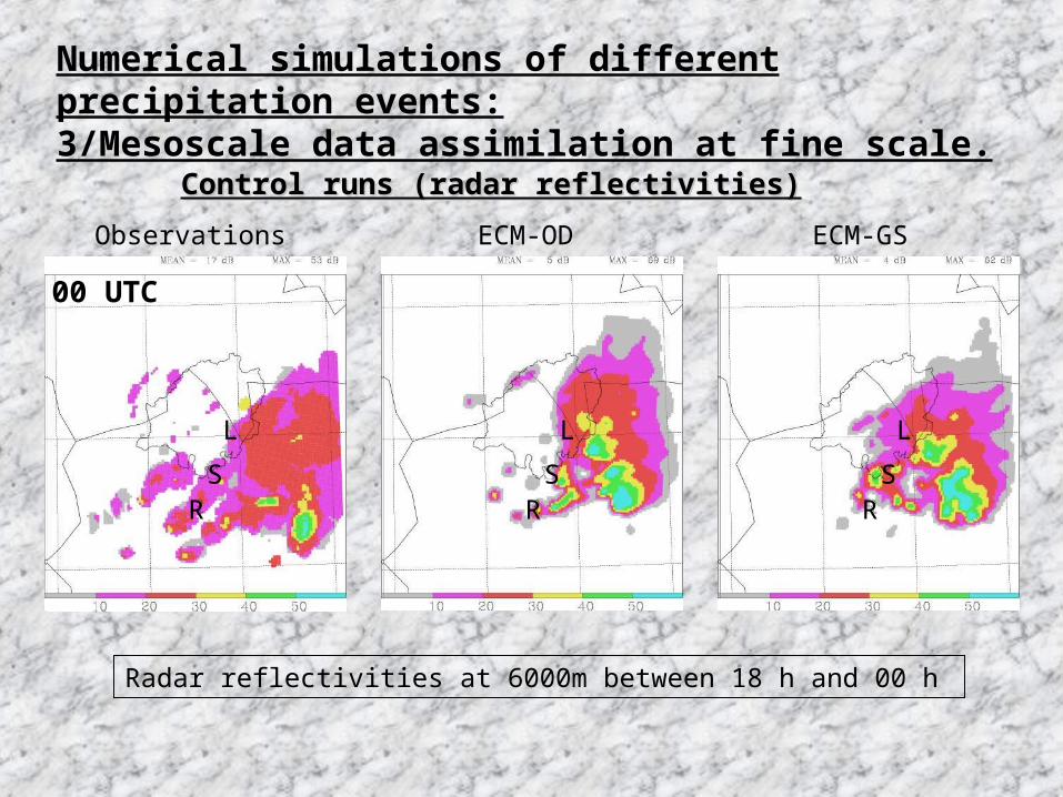
18 UTC19 UTC20 UTC21 UTC22 UTC23 UTC00 UTC

ECM-OD ECM-GSObservations

Radar reflectivities at 6000m between 18 h and 00 h

Control runs (radar reflectivities)Control runs (radar reflectivities)

RS

L

RS

L

RS

L


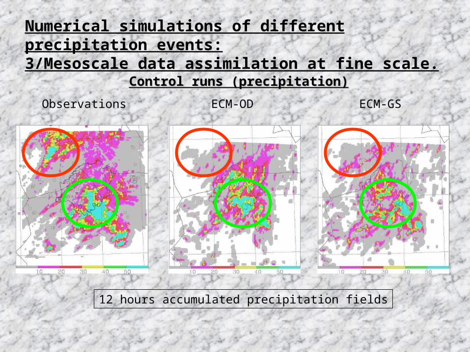
ECM-OD ECM-GSObservations

12 hours accumulated precipitation fields

Control runs (precipitation)Control runs (precipitation)


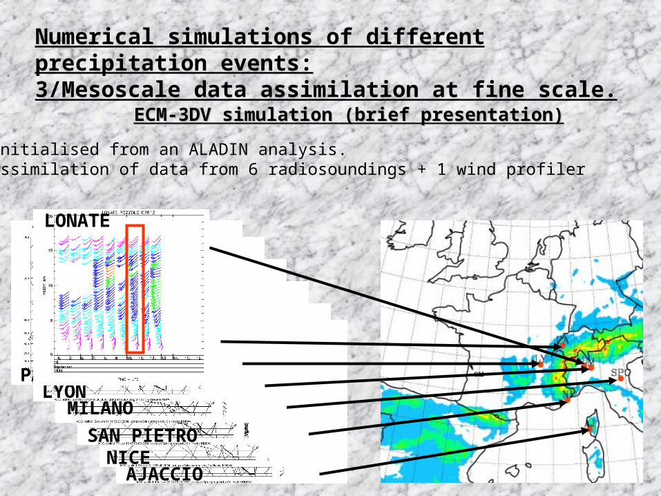
ECM-3DV simulation (brief presentation)ECM-3DV simulation (brief presentation)

AJACCIONICE

SAN PIETRO

MILANOLYON

PAYERNE

LONATE

-Initialised from an ALADIN analysis.-Assimilation of data from 6 radiosoundings + 1 wind profiler


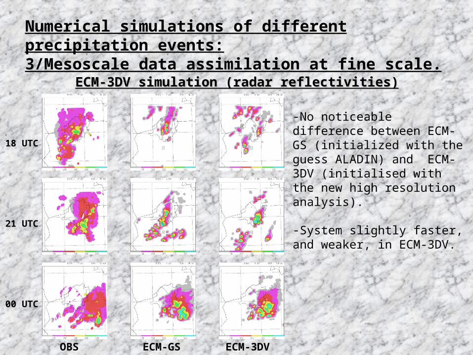
ECM-3DV simulation (radar reflectivities)ECM-3DV simulation (radar reflectivities)

18 UTC

00 UTC

21 UTC

OBS ECM-GS ECM-3DV

-No noticeable difference between ECM-GS (initialized with the guess ALADIN) and ECM-3DV (initialised with the new high resolution analysis).

-System slightly faster, and weaker, in ECM-3DV.


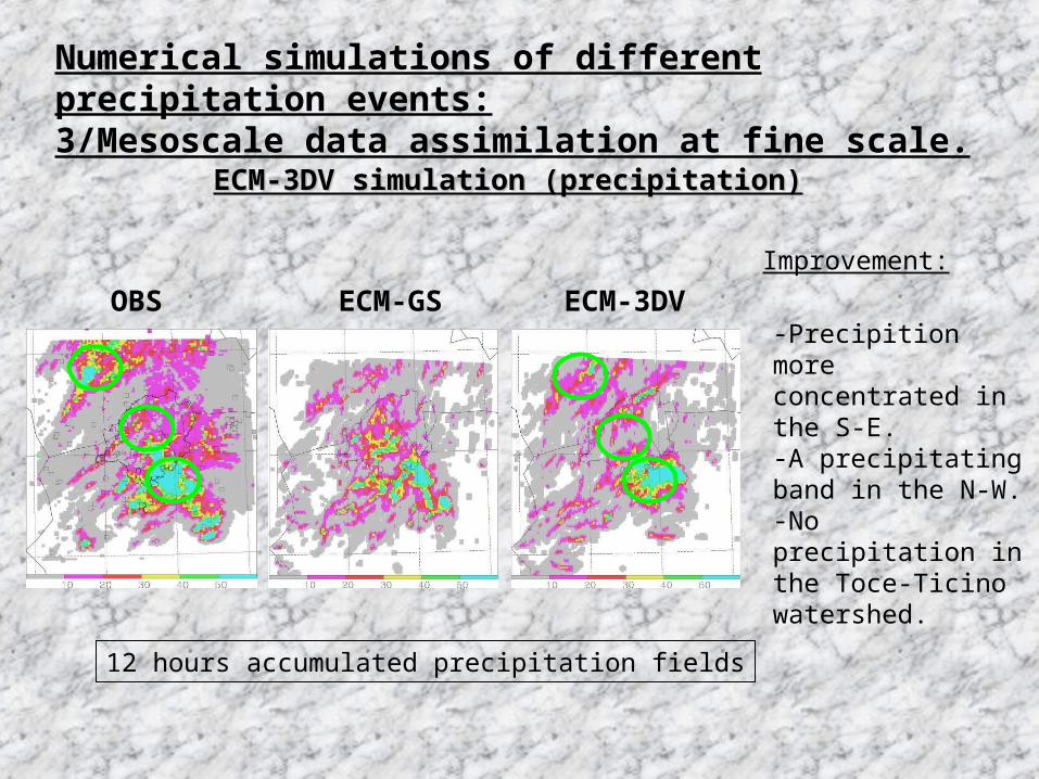
ECM-3DV simulation (precipitation)ECM-3DV simulation (precipitation)

OBS ECM-GS ECM-3DV-Precipition more concentrated in the S-E.-A precipitating band in the N-W.-No precipitation in the Toce-Ticino watershed.

Improvement:

12 hours accumulated precipitation fields


ConclusionsConclusions

-Different numerical simulations of the MAP-IOP2a have been conducted with Meso-NH, with different ALADIN analyses as initial conditions.

-Best results obtained with ECM-3DV, initialized with the new high resolution 3D-VAR ALADIN analysis: ECMWF op. an. as a guess + data assimilation of 6 radiosondes and 1 wind-profiler.

-So far, using the ECMWF reanalysis as a guess did not give any satisfactory results:

observations too far from the forecast fields -> rejected during the assimilation scheme -> insufficient correction.


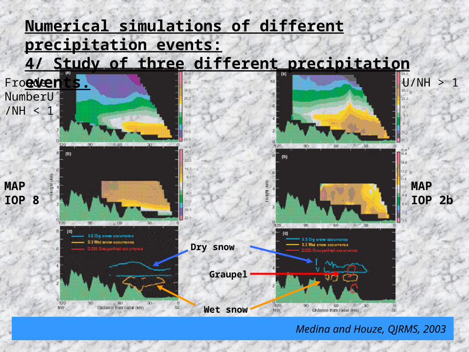
Medina and Houze, QJRMS, 2003

MAPIOP 8

MAPIOP 2b

Froude NumberU/NH < 1

U/NH > 1

Wet snow

Dry snow

Graupel

Numerical simulations of different precipitation events:4/ Study of three different precipitation events.

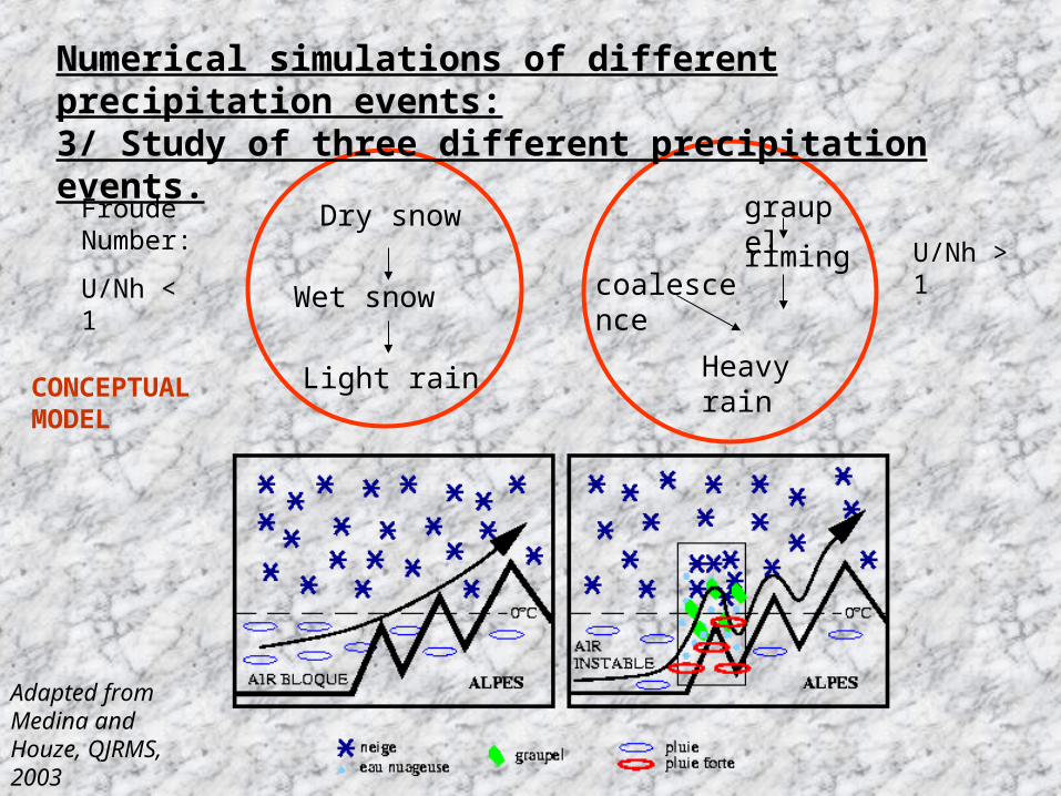
Froude Number:

U/Nh < 1

U/Nh > 1

Dry snow

Wet snow

Light rain

graupel

riming

Heavy rain

coalescence

Adapted from Medina and Houze, QJRMS, 2003


CONCEPTUAL MODEL

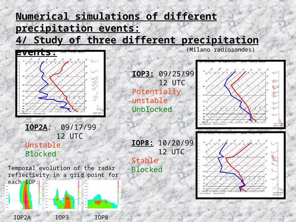
IOP3: 09/25/99 12 UTCPotentially unstableUnblocked

IOP8: 10/20/99 12 UTCStableBlocked

IOP2A: 09/17/99 12 UTC Unstable Blocked

(Milano radiosondes)

IOP2A IOP3 IOP8

Temporal evolution of the radar reflectivity in a grid point for each IOP:


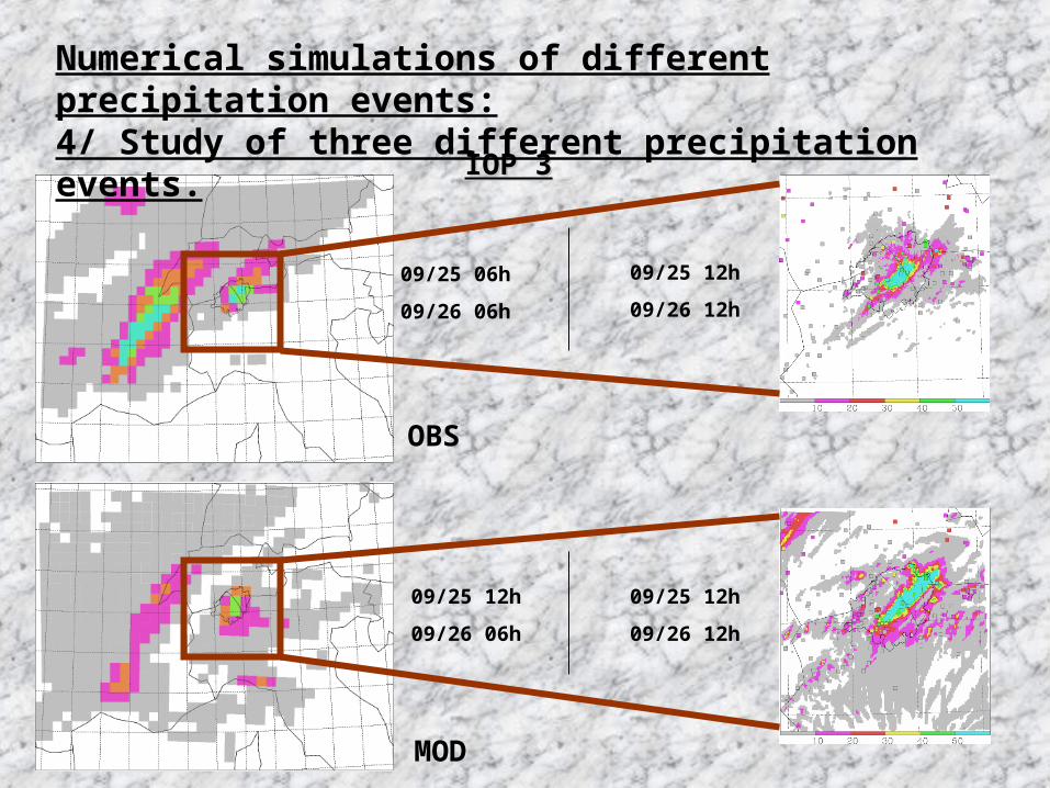
IOP 3IOP 3

OBS

MOD

09/25 06h

09/26 06h

09/25 12h

09/26 06h

09/25 12h

09/26 12h

09/25 12h

09/26 12h


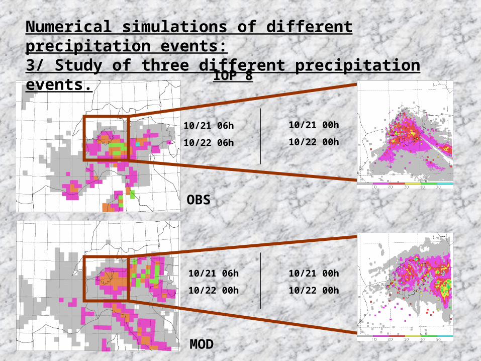
IOP 8IOP 8

OBS

MOD

10/21 06h

10/22 06h

10/21 06h

10/22 00h

10/21 00h

10/22 00h

10/21 00h

10/22 00h


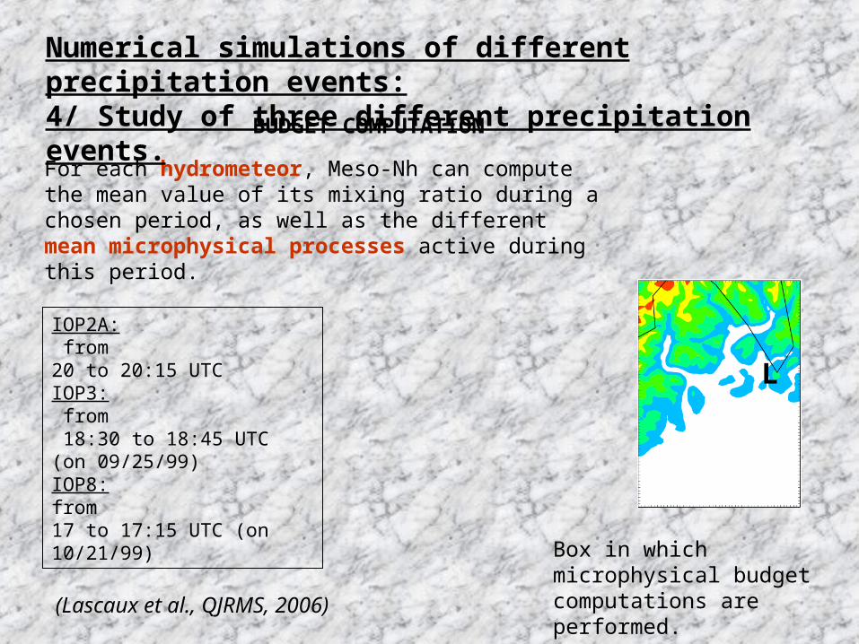
L

IOP2A: from20 to 20:15 UTCIOP3: from 18:30 to 18:45 UTC (on 09/25/99)IOP8:from 17 to 17:15 UTC (on 10/21/99) Box in which

microphysical budget computations are performed.

For each hydrometeor, Meso-Nh can compute the mean value of its mixing ratio during a chosen period, as well as the different mean microphysical processes active during this period.

(Lascaux et al., QJRMS, 2006)


BUDGET COMPUTATION

IOP8

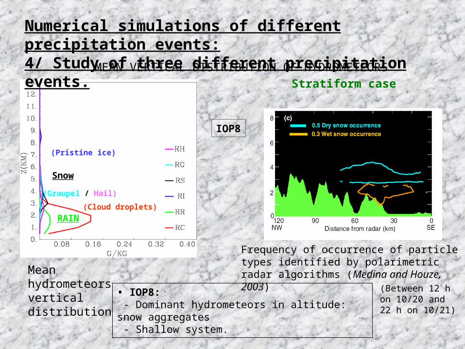
• IOP8: - Dominant hydrometeors in altitude: snow aggregates - Shallow system.

Stratiform case

Mean hydrometeors vertical distribution

Snow

Pristine ice

Rain

(Pristine ice)

Snow

(Graupel / Hail)

RAIN(Cloud droplets)

Frequency of occurrence of particle types identified by polarimetric radar algorithms (Medina and Houze, 2003)

(Between 12 h on 10/20 and 22 h on 10/21)


MEAN VERTICAL DISTRIBUTION OF HYDROMETEORS

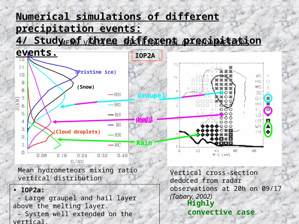
IOP2A

• IOP2a: - Large graupel and hail layer above the melting layer. - System well extended on the vertical.

Highly convective case

Vertical cross-section deduced from radar observations at 20h on 09/17 (Tabary, 2002)

Mean hydrometeors mixing ratiovertical distribution

Glace primaire

Neige

Hail

Graupel Hail

RainRain

Hail

Graupel Hail

(Cloud droplets)

(Pristine ice)

(Snow)



IceSnow

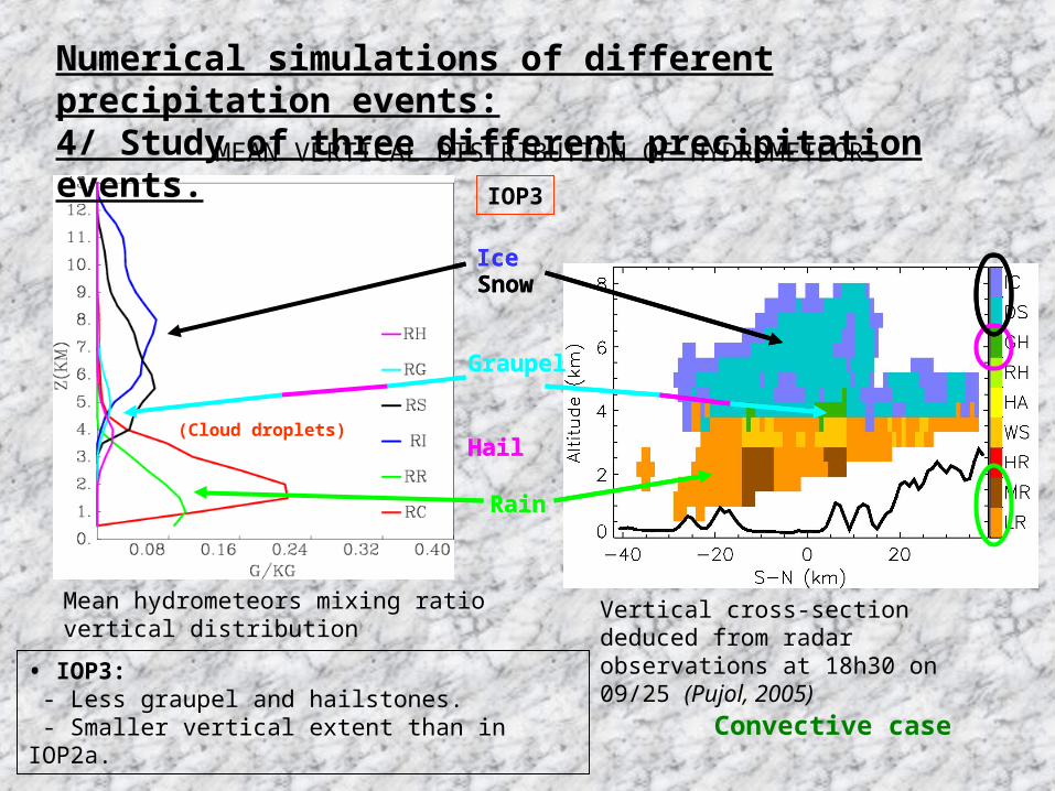
IOP3

• IOP3: - Less graupel and hailstones. - Smaller vertical extent than in IOP2a. Convective case

Vertical cross-section deduced from radar observations at 18h30 on 09/25 (Pujol, 2005)

Mean hydrometeors mixing ratiovertical distribution

Graupel Hail

Rain

Graupel Hail

Rain

(Cloud droplets)

IceSnow



Cloud droplets autoconversion.

Accretion of cloud droplets by raindrops.

s16

10.20

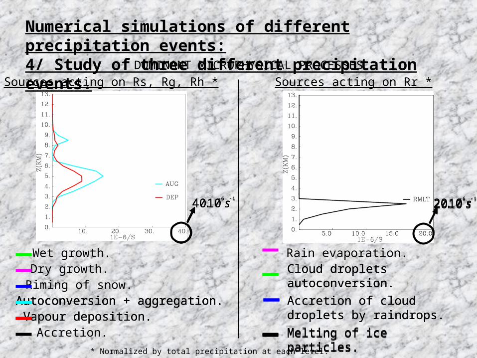
Sources acting on Rs, Rg, Rh * Sources acting on Rr *

* Normalized by total precipitation at each level.

Rain evaporation.Cloud droplets autoconversion.

Accretion of cloud droplets by raindrops.

Melting of ice particles.

s16

10.20

Wet growth.

Riming of snow.Dry growth.

Vapour deposition.Accretion.

s16

10.40

Autoconversion + aggregation.Autoconversion + aggregation.

s16

10.40

Vapour deposition.

s16

10.40

Autoconversion + aggregation.

Melting of ice particles.

s16

10.20


DOMINANT MICROPHYSICAL PROCESSES

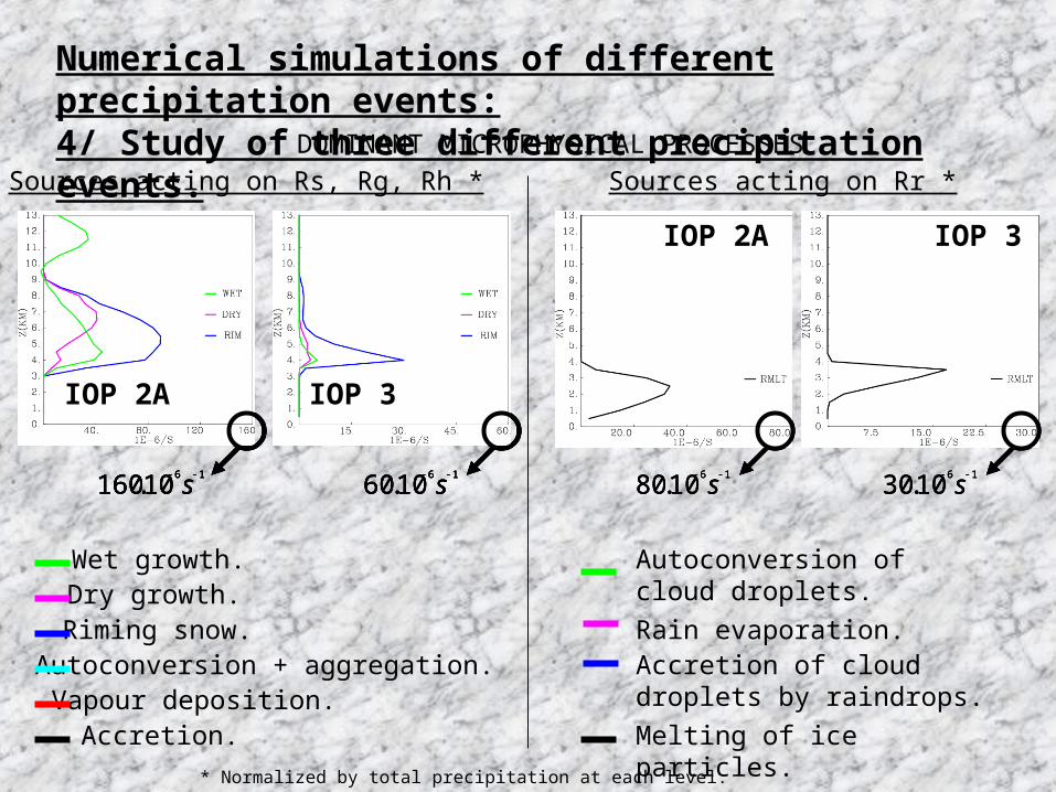
Wet growth. Autoconversion of cloud droplets.Dry growth.Rain evaporation.Riming snow.Accretion of cloud droplets by raindrops.

Autoconversion + aggregation.Vapour deposition.Accretion. Melting of ice particles.

Sources acting on Rs, Rg, Rh * Sources acting on Rr *

* Normalized by total precipitation at each level.

s16

10.160

s16

10.60

s16

10.80

s16

10.30

POI 2A POI 3

IOP 2A IOP 3

s16

10.160

s16

10.60

IOP 2A IOP 3

s16

10.160

s16

10.60

IOP 2A IOP 3

s16

10.160

s16

10.60

IOP 2A IOP 3

s16

10.80

s16

10.30

IOP 2A IOP 3

s16

10.80

s16

10.30

IOP 2A IOP 3


DOMINANT MICROPHYSICAL PROCESSES

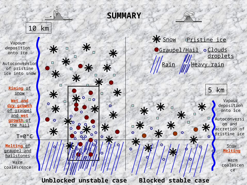
T=0°C

Snow

10 km

5 km

Rain

Graupel/Hail

Pristine ice

Clouds droplets

Riming of snow

Wet and dry growth of graupel and wet

growth of the hail

Melting of graupel and hailstones

Snow Melting

Vapour deposition onto ice

Vapour deposition onto ice

Autoconversion of pristine ice

into snow

Autoconversion and

accretion of pristine ice

Warm coalescence

Warm coalescenc

e

Unblocked unstable case Blocked stable case

Heavy rain

SUMMARY

Documents

What can we do with a mesoscale meteorological model ? Focus on forecasting of heavy precipitation events by Franck Lascaux Keywords: Meso-NH, high resolution,