Embed Size (px)
Citation preview
Finance and Economics Discussion SeriesDivisions of Research & Statistics and Monetary Affairs
Federal Reserve Board, Washington, D.C.
What Can the Data Tell Us About the Equilibrium Real InterestRate?
Michael T. Kiley
2015-077
Please cite this paper as:Kiley, Michael T. (2015). “What Can the Data Tell Us About the Equilibrium Real In-terest Rate?,” Finance and Economics Discussion Series 2015-077. Washington: Board ofGovernors of the Federal Reserve System, http://dx.doi.org/10.17016/FEDS.2015.077.
NOTE: Staff working papers in the Finance and Economics Discussion Series (FEDS) are preliminarymaterials circulated to stimulate discussion and critical comment. The analysis and conclusions set forthare those of the authors and do not indicate concurrence by other members of the research staff or theBoard of Governors. References in publications to the Finance and Economics Discussion Series (other thanacknowledgement) should be cleared with the author(s) to protect the tentative character of these papers.
What Can the Data Tell Us About the EquilibriumReal Interest Rate?
Michael T. Kiley∗
August 26, 2015
Abstract
The equilibrium real interest rate (r∗) is the short-term real interest rate that, inthe long run, is consistent with aggregate production at potential and stable inflation.Estimation of r∗ faces considerable econometric and empirical challenges. On theeconometric front, classical inference confronts the “pile-up” problem. Empirically,the co-movement of output, inflation, unemployment, and real interest rates is tooweak to yield precise estimates of r∗. These challenges are addressed by applyingBayesian methods and examining the role of several “demand shifters”, including assetprices, fiscal policy, and credit conditions. We find that the data provide relativelylittle information on the r∗ data-generating process, as the posterior distribution ofthis process lies very close to its prior. This result contrasts sharply with those for thetrend growth or natural rate of unemployment processes. Second, credit spreads arevery important for the estimated links between output and interest rates and hence forestimates of r∗. Estimates of r∗ that account for this range of considerations are morestable than other estimates, with r∗ at the end of 2014 equal to approximately 1-1/4percent.JEL Classification Code: E5, E3, E4 Keywords: Equilibrium real interest rate, PotentialOutput, Bayesian Methods
∗Office of Financial Stability and Division of Research and Statistics, Federal Reserve Board, Washington,DC 20551. Tel.: (202) 452 2448; E-mail: [email protected]. I would like to thank colleagues and workshopparticipants at the Federal Reserve Board, especially Ed Herbst, Ben Johanssen, and Elmar Mertens, forhelpful comments on earlier drafts. Any views expressed herein are those of the author, and do not reflectthose of the Federal Reserve Board or its staff.

1 Introduction
The equilibrium real interest rate (r∗) is the short-term real interest rate that, in the long
run, is consistent with aggregate production at potential and stable inflation. This concept
enters a range of policy discussions.1 For example, monetary policy discussions focus on r∗
because it provides a gauge of a “neutral” stance of monetary policy.2 However, estimation
of r∗ faces considerable econometric and empirical challenges.
On the econometric front, classical inference confronts the “pile-up” problem. As em-
phasized in Stock and Watson [1996], maximum-likelihood estimation of models in which
a time series contains a small permanent component and a sizable transitory component
tends to drive the estimated role of the permanent component toward zero – that is, the
estimated variance of this component “piles-up” near zero. Because real interest rates
contain (at most) only a small permanent component, the “pile-up” problem is severe in
analyses of the equilibrium real interest rate (Laubach and Williams [2003]). Kim and Kim
[2013] suggest that the “pile-up” problem is much less severe for the Bayesian approach.
This result is closely related to the well-known result that Bayesian inference regarding
unit roots requires no special assumptions, in contrast to the classical approach (e.g., Sims
and Uhlig [1991]). However, the Bayesian approach faces challenges of its own: In partic-
ular, inference depends upon the prior, and researchers may differ in their priors or eschew
the Bayesian perspective altogether (e.g., Stock [1991]). We confront this challenge by
considering sensitivity of the key conclusions to changes in priors regarding the r∗ process.
In the application herein, Bayesian methods aid inference in two ways. First, the fo-
cus on the posterior distribution of the variance of the permanent component provides a
more comprehensive lens with which to examine the range of reasonable settings for this
1For a policy-focused discussion, see the summary of work at the Council of Economic Advisers in Obstfeldand Tesar [2015].
2For example, see Yellen [2015]. While some notion of “equilibrium” real interest rates has a longtradition – dating to at least Knut Wicksell – there are also a number of alternative notions of “equilibrium”,some of which are more short-term and some of which are more long-term. Ferguson [2004] presentsa policymaker’s assessment of how these various definitions contribute to (or confuse) policy discussions.Section 2 below references related research.
1

parameter than the focus on point estimates associated with classical inference. In addi-
tion, the Bayesian approach allows the researcher to impose a prior that the variance of
the permanent component is likely to be non-zero, but not large, and then to assess the
information in the data relative to this prior through examination of the entire posterior
distribution. The comparison of the prior and posterior distributions is a central part of
our examination of the information in the data regarding the r∗ process.
Turning to empirical challenges, the co-movement of output, inflation, unemployment,
and real interest rates is too weak to yield precise estimates of r∗. This is intuitive – if
the relationship were tight, so that most “shocks” to this relationship were shocks to r∗
rather than random noise, then it would be relatively straightforward to “observe” shocks
to r∗ by looking at “errors” in the IS curve. The weak empirical links between output and
interest rates implies an imprecise estimate of the interest-elasticity of demand and large
“errors” in estimated IS curves. Because the models of the equilibrium real interest rate
we consider involve filtering the surprise in the output (and other) equations to estimate
r∗, mis-specification in this equation–such as the omission of important drivers of output–
may substantially affect inference. To address this concern, we examine the role of several
“demand shifters” (including asset prices, fiscal policy, and credit conditions) as influences
on output fluctuations in addition to interest rates.
We reach two primary conclusions. First, the data provide relatively little information
on the r∗ data-generating process; indeed, the posterior distribution of this process lies
very close to the prior distribution. This results contrasts sharply with those for the trend
growth or natural rate of unemployment processes, for which the data are very informa-
tive. Second, additional demand shifters–in particular, a credit spread–are very important
for the estimated links between output and interest rates and hence for estimates of r∗–
implying that previous research that ignores such factors provide poor inference. Estimates
of r∗ that account for this range of considerations are more stable than other estimates,
with r∗ at the end of 2014 equal to approximately 1-1/4 percent.
2

Finally, we also compare auxiliary implications of the models herein to those from the
frequently-cited study of Laubach and Williams [2003]. The models herein yield estimates
of the output gap very similar to those from the Congressional Budget Office, in contrast
to that of Laubach and Williams [2003].
2 Previous Literature on the Equilibrium Real Interest Rate
We have defined the equilibrium real interest rate (r∗) as the level of the real (short-term)
interest rate that is consistent, in the long-run, with output at potential, unemployment at
its natural rate, and inflation at the monetary policymaker’s long-run objective (Laubach
and Williams [2003]). This concept is a long-run notion, and may vary over time because
of changes in the rate of economic growth, the degree of international capital mobility,
or other factors that affect the interest rate that balances savings and investment. In the
approach herein, r∗ is estimated using a “trend/cycle” model.
A variety of approaches have been used to gauge the equilibrium interest rate. One
approach is to examine factors that have contributed to the average level of interest rates
across decades and countries, with guidance from economic theory. For example, Pescatori
and Furceri [2014] and Hamilton, Harris, Hatzius, and West [2015] consider the links
between average real interest rates and factors such as the rate of potential growth in
output (globally or within individual countries) or the global saving rate. Summers [2014]
perceives an imbalance between global saving and investment, stemming in part from
reduced growth prospects in advanced economies, as a motivation for a persistently low
equilibrium real interest rate (and the risk of prolonged “secular stagnation”–that is, a
state in which aggregate demand falls persistently short of aggregate supply).
Laubach and Williams [2003] introduce a relatively simple, trend/cycle approach to
estimate the equilibrium real interest rate. In their model, fluctuations in output and infla-
tion move along an “IS-curve” linking the output gap to the real interest rate and a Phillips
3

curve linking inflation and the output gap. This system treats the level of potential output,
the output gap, and the equilibrium real-interest rate as unobservable state variables, and
derives estimates of these concepts using output, inflation, and the real interest rate as
observable variables via the Kalman filter. Estimates from their model for the U.S. equilib-
rium real interest rate are updated frequently on the website of the Federal Reserve Bank
of San Francisco, and their measure was about -0.4 percent in the fourth quarter of 2014
(as of June 2015).
Clark and Kozicki [2005] highlight a number of challenges associated with the esti-
mation of the equilibrium real interest rate using the trend/cycle approach. First, as em-
phasized in Laubach and Williams [2003], classical inference regarding the equilibrium
interest rate is plagued by the “pile-up” problem associated with estimation of a small per-
manent component of a time series with substantial short-run variation (as discussed in
Stock and Watson [1996]). Second, the filtered estimates of r∗ usually differ substantially
between the “one-sided” and “two-sided” estimates – a result that holds even if the true
population parameters of the model are known because estimation of long-run trends is
more precise after substantial data has been accumulated when time series have impor-
tant short-run components. Finally, “real-time” challenges associated with measurement
and data revisions are substantial. The analysis herein will touch upon the first two issues
(but not “real-time” considerations), and our results regarding the uncertainty regarding
one- and two-sided filtering will largely confirm those of Clark and Kozicki [2005]. For
each of these reasons, Clark and Kozicki [2005] suggest that r∗ estimates may have limited
use in policy discussions.3
The model developed herein draws on the approach of Laubach and Williams [2003].
In particular, the model consists of an IS-curve and Phillips curve. As in Kuttner [1994],
these equations are augmented with an equation linking cyclical fluctuations in unem-
3Orphanides and Williams [2007] analyze this idea in detail, and argue that imprecision in estimatesof r∗ point to a limited role for such estimates in policy discussions. This finding is closely related to thechallenges related to using output gap estimates in policy discussions (e.g., Orphanides and van Norden[2002]).
4

ployment to those in output (i.e., an “Okun’s law” equation).4. This addition nods in the
direction of the literature that emphasizes the role of labor-market indicators in assess-
ments of resource-utilization gaps (e.g., Basistha and Startz [2008] and Fleischman and
Roberts [2011]).
Research has also highlighted the importance of a broad array of financial conditions
in the business cycle: Gilchrist and Zakrajsek [2012] and Kiley [2014a] document impor-
tant contributions of credit spreads to output movements (using, respectively, forecasting
techniques and simple “IS-curve” analysis). Borio, Disyatat, and Juselius [2013] and Ar-
seneau and Kiley [2014] have found that credit measures may improve estimates of the
output gap and natural rate of unemployment. Moreover, the fiscal stance can vary sub-
stantially, with effects on aggregate production and income (Follette and Lutz [2010]).
Simple model-based approaches to estimating r∗ (e.g., Laubach and Williams [2003],
Clark and Kozicki [2005], and Johanssen and Mertens [2015]) have not included such
factors, which may distort their conclusions.5
The equilibrium rate of interest is distinct from the short-run Wicksellian natural rate
of interest, which is the level of the real (short-term) interest rate that is consistent with
price stability in the short-to-medium run (e.g., Woodford [2003] and Edge, Kiley, and
Laforte [2008]). In particular, the natural rate of interest should be expected to fluctuate
considerably over the business cycle, whereas the equilibrium real interest rate is likely
to fluctuate less, if at all, over the business cycle and instead should evolve slowly over
time. (In the literature, the distinction between the equilibrium real interest rate and the
natural rate is not always drawn as finely as herein; as a result, these definitions provide
guidance that should help the reader understand the analysis, but care must be taken when
comparing the discussion herein to that in the broader literature.6)
4A large literature has focused on fluctuations in the unemployment gap and natural rate of unemploy-ment, rather than the output gap; perhaps the most well-known reference is Staiger, Stock, and Watson[1997]
5An alternative approach looks at long-term interest rates to examine movements in r∗, e.g., Bomfim[2001].
6Kiley [2013] notes the long record, emphasized by Paul Samuelson many decades ago, of economists
5
3 Implementation and Results
3.1 The Model
The model includes equations for the dynamics of output y, inflation, ∆p, and the unem-
ployment rate u. Output and the unemployment have permanent, or trend, and cyclical
components. A set of equations governs the cyclical dynamics of inflation π (a Phillips
curve), unemployment u (Okun’s Law), and the output gap y (the IS curve).The cyclical
component of a variable is denoted by a superscript “c” and the trend component by a
superscript “T” (e.g., X = Xc +XT ).
3.1.1 Cyclical Dynamics
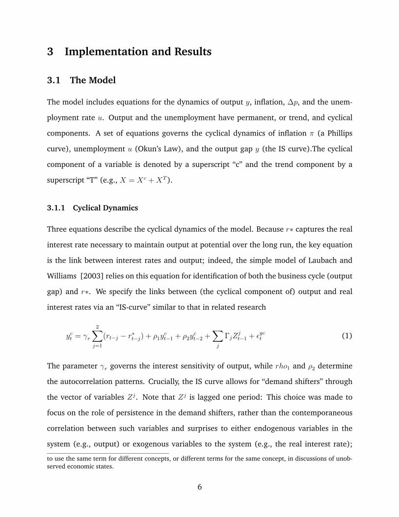
Three equations describe the cyclical dynamics of the model. Because r∗ captures the real
interest rate necessary to maintain output at potential over the long run, the key equation
is the link between interest rates and output; indeed, the simple model of Laubach and
Williams [2003] relies on this equation for identification of both the business cycle (output
gap) and r∗. We specify the links between (the cyclical component of) output and real
interest rates via an “IS-curve” similar to that in related research
yct = γr
2∑j=1
(rt−j − r∗t−j) + ρ1yct−1 + ρ2y
ct−2 +
∑j
ΓjZjt−1 + εyct (1)
The parameter γr governs the interest sensitivity of output, while rho1 and ρ2 determine
the autocorrelation patterns. Crucially, the IS curve allows for “demand shifters” through
the vector of variables Zj. Note that Zj is lagged one period: This choice was made to
focus on the role of persistence in the demand shifters, rather than the contemporaneous
correlation between such variables and surprises to either endogenous variables in the
system (e.g., output) or exogenous variables to the system (e.g., the real interest rate);
to use the same term for different concepts, or different terms for the same concept, in discussions of unob-served economic states.
6

for example, lagging credit spreads abstracts from any contemporaneous relationship be-
tween the output gap, real interest rates, and spreads. This reduced-form approach does
not take a stand on the underlying structural model, and the results below will highlight
the importance of understanding credit spreads. Nonetheless, the results were essentially
identical whether Zj entered with a lag or contemporaneously. Finally, our analysis will in-
clude a specification without demand shifters, and one in which a (lagged) corporate bond
spread, credit growth, and fiscal impetus enter. A more complete description of these vari-
ables and the motivation for their inclusion follows in the next subsection on data and
empirical analysis.
Unemployment is determined by Okun’s law
uct = −β(0.4yct + 0.3yct−1 + 0.2yct−2 + 0.1yct−3
)+ εut . (2)
Note that the equation assumes that unemployment gap fluctuations are a (fixed) dis-
tributed lag of output gap fluctuations, capturing the well-known tendency for unemploy-
ment to lag movements in output. This relationship is drawn from Braun [1990].
Inflation dynamics are governed by
πt = s1πt−1 + s2
∑4j=2 πt−j
3+ (1− s1 − s2)Et−1π
LR + αuuct +∑j
BjXjt + επt . (3)
In the Phillips curve, inflation is a influenced by the unemployment gap, its own lags, and
the level of long-run inflation expectations. The role for long-run inflation expectations
in the Phillips curve has considerable empirical support (e.g., Kiley [2014a] and Kiley
[2014b]), and survey measures of long-run inflation expectations will be used in the
empirical analysis. The model also allows for an influence on inflation from other factors
(Xj). Following Arseneau and Kiley [2014] and Gilchrist et al [2013], we will include
credit conditions in Xj, potentially capturing the notion that such conditions act as a “cost-
push” factor on price inflation. Results are not sensitive to inclusion of this factor.
7
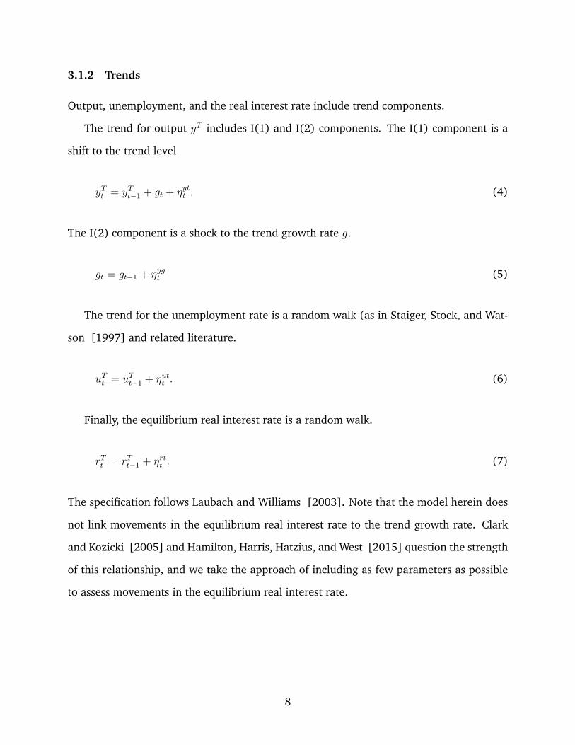
3.1.2 Trends
Output, unemployment, and the real interest rate include trend components.
The trend for output yT includes I(1) and I(2) components. The I(1) component is a
shift to the trend level
yTt = yTt−1 + gt + ηytt . (4)
The I(2) component is a shock to the trend growth rate g.
gt = gt−1 + ηygt (5)
The trend for the unemployment rate is a random walk (as in Staiger, Stock, and Wat-
son [1997] and related literature.
uTt = uTt−1 + ηutt . (6)
Finally, the equilibrium real interest rate is a random walk.
rTt = rTt−1 + ηrtt . (7)
The specification follows Laubach and Williams [2003]. Note that the model herein does
not link movements in the equilibrium real interest rate to the trend growth rate. Clark
and Kozicki [2005] and Hamilton, Harris, Hatzius, and West [2015] question the strength
of this relationship, and we take the approach of including as few parameters as possible
to assess movements in the equilibrium real interest rate.
8
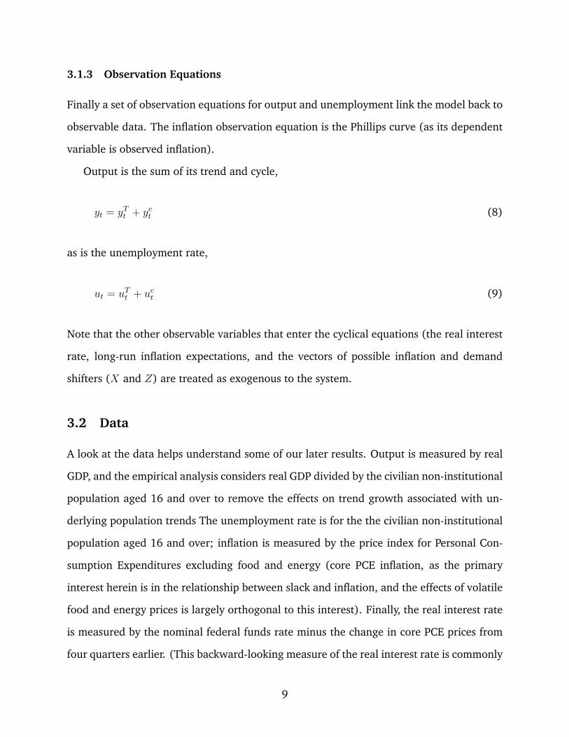
3.1.3 Observation Equations
Finally a set of observation equations for output and unemployment link the model back to
observable data. The inflation observation equation is the Phillips curve (as its dependent
variable is observed inflation).
Output is the sum of its trend and cycle,
yt = yTt + yct (8)
as is the unemployment rate,
ut = uTt + uct (9)
Note that the other observable variables that enter the cyclical equations (the real interest
rate, long-run inflation expectations, and the vectors of possible inflation and demand
shifters (X and Z) are treated as exogenous to the system.
3.2 Data
A look at the data helps understand some of our later results. Output is measured by real
GDP, and the empirical analysis considers real GDP divided by the civilian non-institutional
population aged 16 and over to remove the effects on trend growth associated with un-
derlying population trends The unemployment rate is for the the civilian non-institutional
population aged 16 and over; inflation is measured by the price index for Personal Con-
sumption Expenditures excluding food and energy (core PCE inflation, as the primary
interest herein is in the relationship between slack and inflation, and the effects of volatile
food and energy prices is largely orthogonal to this interest). Finally, the real interest rate
is measured by the nominal federal funds rate minus the change in core PCE prices from
four quarters earlier. (This backward-looking measure of the real interest rate is commonly
9

Figure 1: Key Data Series: Output, Unemployment, Inflation, and the Real Interest Rate
Source: Real GDP and PCE prices, Bureau of Economic Analysis; Unemployment Rate, Bu-reau of Labor Statistics; Federal Funds Rate, Federal Reserve Board. Inflation and real inter-est rate computed by author. Data accessed from Federal Reserve FRB/US database availableat http://www.federalreserve.gov/econresdata/frbus/us-models-package.htm. Data accessed July2, 2015. Shaded regions indicate recessions as identiied by the National Bureau of EconomicResearch.
used in related studies.)7
Focusing first on variables common to trend/cycle models and as reported in figure
1, the unemployment rate shows a clear cycle around recessions (as identified by the
National Bureau of Economic Research); this cycle, in conjunction with Okun’s Law, is
highly informative about the overall business cycle. Indeed, a casual look at the change
in real GDP illustrates how difficult it would be to gauge the state of overall resource
7Real GDP and the core PCE price index are from the Bureau of Economic Analysis; Population and theunemployment rate are from the Bureau of Labor Statistics; and the nominal federal funds rate is from theFederal Reserve Board. All data are taken from the Federal Reserve’s FRB/US model database, including anyadjustments made by Federal Reserve staff. Brayton, Laubach, and Reifschneider [2014] describes the mostrecent FRB/US model and an easily-accessible version of the data.
10

utilization without labor market data. Inflation has a highly persistent component over
the period since 1960, but has been fairly stable around 2 percent for the two decades
leading up to 2014. Finally, the real interest rate appears to have both a clear cyclical
component and a lower frequency component–consistent with the general idea that there
may be some trend component to the real interest rate.
As additional control variables, we consider three time series that capture factors pre-
vious research or commentary has suggested are important for fluctuations in output and
which may be particularly important in assessments or r∗: A corporate bond spread, ag-
gregate credit growth, and the impetus to demand from fiscal policy. A large literature
documents that corporate bond spreads have important information for forecasting output
or as a shifter in an IS curve (e.g., Gilchrist and Zakrajsek [2012] and Kiley [2014a]). As
shown in figure 2, this spread tends to rise during recessions. Moreover. it was notably
below average in the late 1990s and mid-2000s: This observation call to mind the notion
from Summers [2014] that the full-employment periods experienced in the late 1990s
and mid-2000s were supported by easy financial conditions (“bubbles”), which Summers
[2014] suggests may have masked a trend decline in the equilibrium real interest rate.
Finally, this spread has bee unusually high from the financial crisis of 2008 through 2014
and only returned to near its average level in 2014.
The middle panel presents aggregate credit growth (relative to GDP): Borio, Disyatat,
and Juselius [2013] and Arseneau and Kiley [2014] suggest rapid credit growth was an
impetus to the business cycle. Lo and Rogoff [2015] and Rogoff [2015] cast doubt on
views of “secular stagnation” and instead view the slow recovery and low level of interest
rates in recent years to the deleveraging process. According to this view, demand will
recover more notably when credit growth returns to normal–and the middle panel suggests
that credit growth had approached a more typical level, relative to GDP, by late 2014.
Finally, the lower panel reports the fiscal impetus measure of Follette and Lutz [2010]:
This measure captures the “exogenous” impetus to GDP from fiscal policy. Such a construc-
11

Figure 2: Key Data Series: A Corporate Bond Spread, Credit Volumes, and Fiscal Impetus
Source: Private Nonfinancial Credit Relative to Nominal GDP, Federal Reserve Board (FinancialAccounts of the United States, http://www.federalreserve.gov/releases/z1/Current/) and Bureauof Economic Analysis; Corporate bond spread, Author’s computation based on 10-year Treasuryyield and Corporate bond yield from Federal Reserve’s FRB/US model database (available athttp://www.federalreserve.gov/econresdata/frbus/us-models-package.htm. Data accessed July 2,2015); Fiscal impetus from Follette and Lutz [2010]. Shaded regions indicate recessions as iden-tified by the National Bureau of Economic Research.
tion is fraught with controversy, as it includes both direct, discretionary spending measures
and assumptions on how tax changes flow though to spending. Because this measure is
controversial, we will explore results with and without this measure. Setting these contro-
versies aside, the fiscal impetus measure has been a notable drag on spending since 2011
and remained far below its typical level in 2014, consistent with the common view that the
shift toward a contractionary fiscal stance at that time has been a factor in the relatively
tepid pace of economic growth (e.g., Bernstein [2014]).
12
3.3 Estimation
3.3.1 Estimation Strategy
Output, inflation, unemployment, the real interest rate, and any additional controls are ob-
served variables. Output, inflation, and the unemployment are endogenous in the model,
and other controls are treated as exogenous. This follows Laubach and Williams [2003]
and Clark and Kozicki [2005]. (An obvious extension is to treat other observables as
“endogenous” within the model. Johanssen and Mertens [2015] pursue this idea by in-
cluding a specification for the endogenous evolution of the short-term interest rate. We do
not adopt this approach, and discuss problems that arise by treating control variables as
exogenous in subsequent sections.)
The errors in all equations are assumed to follow a Normal distribution, implying that
the Kalman filter is the optimal method for parsing the data into trend and cycle. We
construct the likelihood of the data via the Kalman filter.
A long literature has emphasized that estimation of “trend/cycle” decompositions via
maximum likelihood is problematic because the variance of the trend processes for eco-
nomic growth “pile-up” near zero (Stock and Watson [1996]). Bayesian methods do not
face the same problems (Kim and Kim [2013]). As earlier work on r∗ has noted the em-
pirical challenges associated with the pile-up problem, a Bayesian approach is attractive.
In addition, a Bayesian approach allows imposition of prior views that capture common
discussions in the literature, and a clear discussion of the information in the data through
comparison of the prior and posterior distributions.
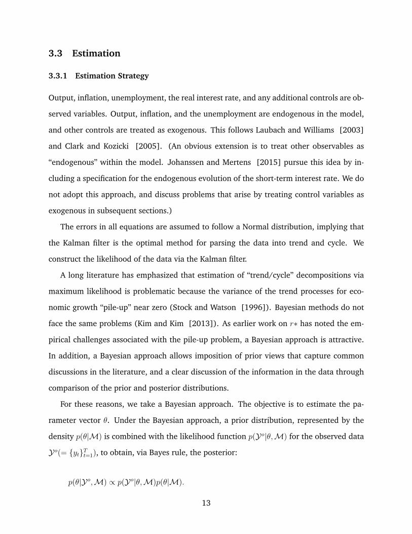
For these reasons, we take a Bayesian approach. The objective is to estimate the pa-
rameter vector θ. Under the Bayesian approach, a prior distribution, represented by the
density p(θ|M) is combined with the likelihood function p(Yo|θ,M) for the observed data
Yo(= {yt}Tt=1), to obtain, via Bayes rule, the posterior:
p(θ|Yo,M) ∝ p(Yo|θ,M)p(θ|M).
13
To facilitate estimation, we must access the posterior p(θ|Yo,M). Unfortunately, the pos-
teriors are analytically intractable, owing to the complex ways θ enters the likelihood
function. To produce draws from the posteriors, we resort to Markov-Chain Monte Carlo.8
We employ a Normal(0,2) prior for all “cyclical” parameters in the equations. Given
the scaling of variables in the model, this prior is fairly uninformative.
The priors for the standard errors of the cyclical and trend equations assume an In-
verted Gamma distribution. For the errors in the cyclical equations, we assume means and
standard errors of 2; the exception is the error in Okun’s aw, which is assumed to have a
mean and standard deviation of 0.25. For the trend errors, we assume means and standard
errors of 0.25. These assumptions imply the prior view that fluctuations in trend growth,
r∗, UT are modest relative to cyclical variation. Our subsequent analysis will compare
these prior distributions with the posterior distributions to highlight the information in the
data for r∗.
3.3.2 Results
Our estimation sample spans from 1960Q1 to 2014Q4. We present results for three speci-
fications:
• Case 1 – No controls (as in Laubach and Williams [2003] and Clark and Kozicki
[2005]): In this case, both X and Z are empty.
• Case 2 – Only credit spread control: In this case, corporate bond spreads are the only
element of Z and X is empty.
• Case 3 – All controls: In this case, Z includes the corporate bond spread, credit
growth (with household and business credit separated), and fiscal impetus.9
8All our estimation procedures use Dynare (Adjemian et al [2011]).9The credit variable is credit growth, measured as the quarterly percent change. It is assumed that it is
this growth rate relative to trend growth g that influences the output gap.
14

The parameters governing dynamics are reported in table 1 and the standard errors of
the shocks to each equation are reported in table 2.
Case 1 - No controls Case 2-Bond Spread Case 3- All controlsMean s.d. Mean s.d. Mean s.d.
IS curveρ1 1.330 0.1008 0.920 0.1071 0.838 0.0961ρ2 -0.376 0.0998 0.037 0.0977 -0.016 0.0859γr 0.076 0.0340 0.111 0.0357 0.126 0.0297ΓSpread - - -0.549 0.0991 -0.494 0.0929ΓFiscal - - - - -0.047 0.1850ΓCredit,Bus - - - - 0.043 0.0161ΓCredit,HH - - - - 0.022 0.0134Okun’s Lawβ -0.578 0.0455 -0.581 0.0457 -0.566 0.0440Phillips Curves1 0.632 0.0706 0.637 0.0705 0.644 0.0780s2 0.151 0.0825 0.179 0.0821 0.182 0.0818αu -0.073 0.0528 -0.089 0.0417 -0.087 0.0564BCredit,Bus - - - - 0.004 0.0202
Table 1: Moments of Posterior Distributions of Parameters for Dynamic Equations
Several results are apparent. As shown in the first two columns, the system without any
controls has relatively typical properties: The AR(2) process for output shows a coefficient
on the first lag (ρ1) greater than one and a negative coefficient on the second lag (ρ2)
; the coefficient on the output gap in the Okun’s law equation (β) is near (but slightly
greater than) 1/2 (similar to Fleischman and Roberts [2011], and the estimated mean
and standards error of the posterior distribution for the Phillips curve relationship between
inflation and unemployment suggests that unemployment is not strongly associated with
downward pressure on inflation (αu > 0, but small and estimated somewhat imprecisely).
The importance of the control variables can be seen in columns 3-6, which report cases
2 and 3. Note that the lagged credit spread is strongly associated with cyclical move-
ments in output. In addition, the interest sensitivity of the output gap is larger and more
precisely estimated in the presence of the controls. Finally, fiscal impetus is not signifi-
15
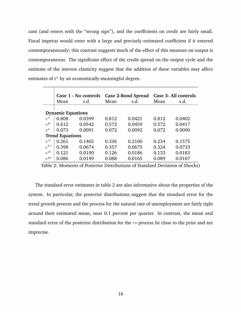
cant (and enters with the “wrong sign”), and the coefficients on credit are fairly small.
Fiscal impetus would enter with a large and precisely estimated coefficient if it entered
contemporaneously; this contrast suggests much of the effect of this measure on output is
contemporaneous. The significant effect of the credit spread on the output cycle and the
estimate of the interest elasticity suggest that the addition of these variables may affect
estimates of r* by an economically-meaningful degree.
Case 1 - No controls Case 2-Bond Spread Case 3- All controlsMean s.d. Mean s.d. Mean s.d.
Dynamic Equationseπ 0.808 0.0399 0.812 0.0421 0.812 0.0402eyc 0.612 0.0542 0.572 0.0459 0.572 0.0417eu 0.073 0.0091 0.072 0.0092 0.072 0.0090Trend Equationsert 0.261 0.1465 0.336 0.2160 0.234 0.1575eY t 0.398 0.0674 0.357 0.0675 0.324 0.0733eut 0.121 0.0190 0.126 0.0186 0.133 0.0183eyg 0.086 0.0149 0.088 0.0165 0.089 0.0167
Table 2: Moments of Posterior Distributions of Standard Deviation of Shocks)
The standard error estimates in table 2 are also informative about the properties of the
system. In particular, the posterior distributions suggest that the standard error for the
trend growth process and the process for the natural rate of unemployment are fairly tight
around their estimated mean, near 0.1 percent per quarter. In contrast, the mean and
standard error of the posterior distribution for the r∗ process lie close to the prior and are
imprecise.
16

4 Implications of the Estimation Results
4.1 The Information in the Data
To illustrate the degree of precision, relative to the prior, in the posterior distribution of
the r∗ process. figures 3 and 4 plot the prior and posterior distributions for the standard
error of the low-frequency components of r∗, g, and UT for case 1 and case 3.
Figure 3: Prior and Posterior Distributions of Standard Errors of Trends: Case 1
Source: Author’s computations from model estimates.
The results are similar across cases. The posterior distribution for r∗ is about as diffuse
and centered on similar values as the prior distribution, indicating that the data contain
relatively little information about the r∗ process. This result contrasts sharply with those
for the g∗ and UT processes, where the posterior distribution is much tighter than the prior
distribution.
17

Figure 4: Prior and Posterior Distributions for Standard Errors of Trends: Case 3
Source: Author’s computations from model estimates.
These results suggest that researchers with alternative prior views about the degree
to which r∗ has shifted over time are unlikely to be swayed by the information in the
relationship between output and short-term interest rates–there is simply too little infor-
mation in such co-movement over the past 50 years to provide much guidance. This result
is very loosely related to the challenges associated with classical inference and r∗ estima-
tion, where researchers have noted sharp distinctions between maximum likelihood and
median-unbiased estimates of the r∗ process (e.g., Laubach and Williams [2003] and
Clark and Kozicki [2005]).
To illustrate the role of the prior in shaping parameter estimates, three robustness
checks were considered. First, following the suggestion in Mueller [2012], we shifted
the prior mean of each of the standard deviations for the trends by one (prior) standard
18
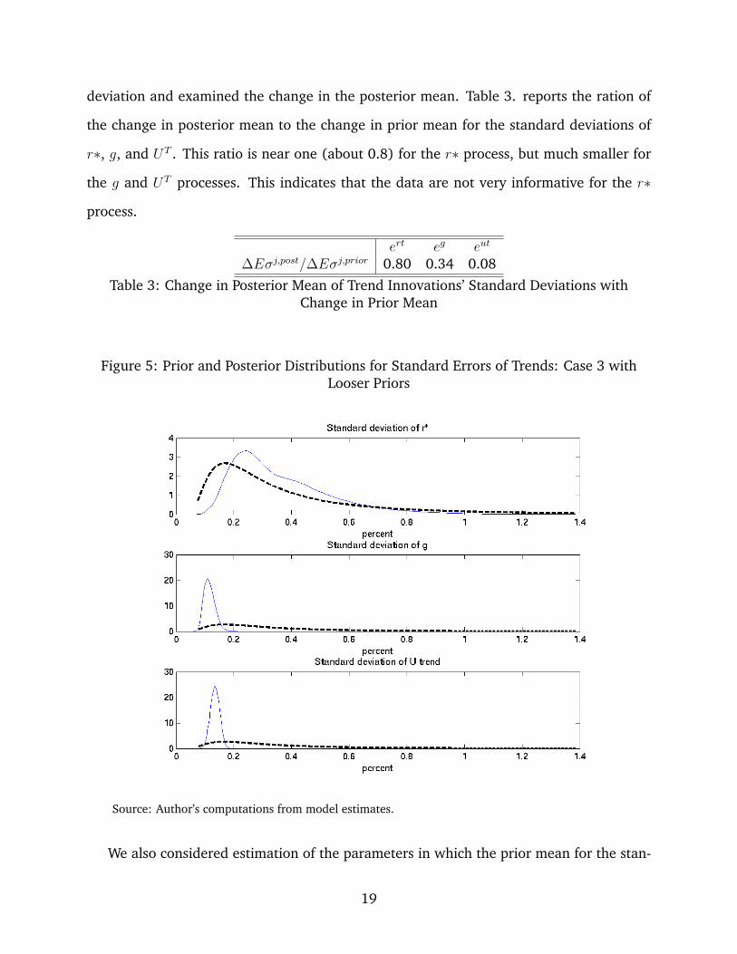
deviation and examined the change in the posterior mean. Table 3. reports the ration of
the change in posterior mean to the change in prior mean for the standard deviations of
r∗, g, and UT . This ratio is near one (about 0.8) for the r∗ process, but much smaller for
the g and UT processes. This indicates that the data are not very informative for the r∗
process.
ert eg eut
∆Eσj,post/∆Eσj,prior 0.80 0.34 0.08Table 3: Change in Posterior Mean of Trend Innovations’ Standard Deviations with
Change in Prior Mean
Figure 5: Prior and Posterior Distributions for Standard Errors of Trends: Case 3 withLooser Priors
Source: Author’s computations from model estimates.
We also considered estimation of the parameters in which the prior mean for the stan-
19

dard deviations of the trends were held at 0.25, but the standard deviation of the prior was
increased to 5 (from 0.25). Figure 5 compares the estimated of the priors and posteriors
for the standard deviations of r∗, g, and UT . As before, the posterior for r∗ resembles the
prior, while those for the other trend processes are informed by the data.
Figure 6: Prior and Posterior Distributions for Standard Errors of Trends: Case 3 withAlternative Prior Shape
Source: Author’s computations from model estimates.
Finally, we examined priors with a different shape. As should be apparent in the figures
shown so far, the (inverted Gamma) priors for the standard deviations of the trends have
peaks away from zero and place low probability on the possibility that the innovations for
the trend have a very low variance. To explore the sensitive of the results for the trend
processes to this prior, we considered priors for the standard deviations of r∗, g, and UT
that peak near zero (and have the same prior mean). In particular, we assumed a Beta
20
distribution for these parameters. Plots of the priors and posteriors under this assumption
are shown in figure -6. As before, the posterior for the standard deviation of r∗ lies very
close to the prior, whereas the data appear quite informative about the g and UT processes.
4.2 Estimates of r*
While the process for r∗ is closely related to the assumed prior distribution, this prior cap-
tures the common view (as captured in the literature developing and using r∗) that there
may be some low frequency component to the equilibrium short-term real interest rate. As
a result, examination of the model’s estimate of r∗ and the range of estimates consistent
with the posterior distribution of the model’s parameters carries information about both
where the equilibrium rate may currently stand and the degree to which alternative views
are “reasonable” in light of the model. Figure -7 presents the smoothed (or two-sided)
estimate of r* from case 3 (all controls) along with the 68-percent confidence set based on
the posterior distribution of model parameters.10
As illustrated by the comparison of the black and blue-dashed line (as well as the
associated confidence set), the overwhelming share of movements in the real interest rate
are viewed by the model as movements around r∗, with only modest movements in r∗.
From the early 1960s through the 1980s, r∗ is estimated to lie near 2 percent, close to the
equilibrium rate assumed in the now-classic analysis of monetary policy rules in Taylor
[1993]. At the end of 2014, the point estimate of r∗ equaled 1-1/4 percent
The green-starred line in figure -7 represents the estimate of r∗ from case 1, without
controls in the IS curve. Two results are apparent. First, the estimate from the model
without controls usually falls outside the confidence set from case 3– which is another ex-
10This confidence set describes the range of point estimates for r∗ implied by the distribution of coeffi-cients. It is not a complete description of uncertainty. In particular, this assessment abstracts from filteringuncertainty – that is, the inherent uncertainty associated with extracting an unobserved variable via theKalman filter for known parameters. However, this notion of confidence is what is relevant for comparingresults across models, as it indicates whether the coefficients from a model are “close” to those implied bythe posterior distribution.
21

Figure 7: Estimate of r∗
Source: Author’s computations from model estimates.
pression of the finding that the controls are important for describing output gap dynamics
and the model without controls lies a far distance from the posterior distribution of the
model with controls. (In principle, this need not have been the case, as case 1 is a special
case of the general model, and the prior distribution for all of the parameters is centered,
loosely, on case 1.)
In addition, it is evident that the estimate of r∗ absent controls is somewhat more vari-
able than that with controls – that is, the controls appear to pick up some of the business-
cycle frequency movements affecting the IS curve that models absent controls may tend
to attribute to movements in r∗. In addition, the model without controls estimates that r∗
has fallen to a very low level since 2008, whereas the model with controls put r∗ at 1-1/4
percent – a level modestly below that estimated for earlier decades.
22

This difference in results between models with and without controls raises a central
question – to what extent is the model estimating a notion of the “equilibrium rate” that
is relevant. The answer to this question depends upon the circumstances. In particular,
the control variables are treated as exogenous in the model herein, and any comparison
of estimates of the equilibrium real interest rate from the model must consider the cur-
rent values of the control variables in light of historical norms for such variables. When
evaluating this situation, the state of the credit spread is the key factor, as it plays the dom-
inant role among the control factors. In this regard, it is notable from figure -2 that the
corporate bond spread essentially equaled its average over the estimation period, in sharp
contrast to readings for this variable in the six years prior to 2014. Because this variable
is the main control variable influencing r∗. it may be reasonable to expect the estimated
value of r∗ at end-2014 of 1-1/4 percent to be a plausible candidate for the equilibrium
short-term interest rate over the long run. That said, the value of short-term interest rates
compatible with output at potential in the short run will be influenced by many factors.
This assessment is made very clear by the explicit consideration of control variables in our
model, but is equally true of models that omit relevant factors in their empirical analysis.
4.3 Comparison to Laubach and Williams Results
Indeed, the simpler models analyzed in Laubach and Williams [2003] and Clark and
Kozicki [2005] omit any controls. While this approach avoids the challenge of interpreting
the state of controls relative to historical values or likely values in the future, it potentially
omits important information. As a result, it is useful to examine the estimates from the
model herein to that produced by the Laubach and Williams [2003] model (figure 8). As
in figure 7, the black and blue-dashed lines present the data and r∗ estimate from case 3,
respectively, while the shaded region is the 68-percent confidence set. The green-starred
23

Figure 8: Estimate of r∗ from Laubach and Williams [2003]
Source: Author’s computations from model estimates and Federal Reserve Bank of San Francisco(http://www.frbsf.org/economic-research/economists/john-williams/).
line is the estimate from Laubach and Williams [2003].11
The comparison illustrates clearly that the models herein behave quite differently from
Laubach and Williams [2003]–both over history, and in the recent sample (where the
Laubach and Williams [2003] estimate of r∗ falls to nearly −1/2 percent by end-2014, as
compared to 1-1/4 percent for the case-3 model. Indeed, the confidence set suggests that
there are not likely coefficient combinations for the specification herein that would lead to
estimates similar to those in Laubach and Williams [2003].
The dis-similarity of results partially reflects the role of control variables, and the chal-
lenges of interpreting r∗ in the presence of control variables that were discussed in the
11This is the two-sided estimate as reported on the website of the Federal Reserve Bank of San Franciscoas of June, 2015.
24

previous subsection. Nonetheless, the models are give quite different results over most of
the sample period even abstracting from control variables, as is evident from a comparison
of the green-starred lines in figures 7 and 8. This is not especially surprising – the model
herein uses more data (output, inflation, unemployment, and real interest rates vs. output,
inflation, and real interest rates), a different Phillips curve (with a role for long-term in-
flation expectations), a different estimation sample (including the Great Recession in this
analysis, vs. a sample period ending in 2000) , and a Bayesian approach. Each of these
factors plays some role in accounting for differences.
4.4 Auxiliary Implications of Models
A more direct assessment of the economic implications of these differences can be seen
by comparing auxiliary implications of the models. An especially interesting comparison
of differences across frameworks can be seen in alternative assessments of the output gap
from different frameworks.
Figure -9 presents the estimate of the output gap from the Congressional Budget Office,
the case-3 model (which is very similar to that from all specifications analyzed herein), and
the Laubach and Williams [2003] model. (The shaded region is the 68-percent confidence
set associated with coefficient uncertainty; as above, filter uncertainty is not the focus
herein, but is important for all methods). The figure illustrates the similarity in assessments
of resource utilization from the early 1960s through about the year 2000 (the end of the
estimation sample in Laubach and Williams [2003]). After that period, the CBO and
model yield similar assessments of the output gap, but the Laubach and Williams [2003]
model is quite different. For example, output is only slightly below potential in 2009
according to the Laubach and Williams [2003] model, but is very far below potential in the
alternative assessments. One factor contributing to these different assessments is the role
of the unemployment rate, which is central in research on the trend/cycle decomposition
of output (e.g., Basistha and Startz [2008] and Fleischman and Roberts [2011]).
25

Figure 9: Estimate of Output Gap from CBO, Case 3, and Laubach and Williams [2003]
Source: Author’s computations from model estimates and Congressional BudgetOffice (https://www.cbo.gov/sites/default/files/cbofiles/attachments/45066-2015-07-EconomicDataProjections.xlsx).
5 Conclusion
Our analysis points to two central conclusions.
First, the data provide relatively little information on the r∗ data-generating process, as
indicated by a posterior distribution for the r∗ process that looks like the prior distribution
we have assumed. This suggests some caution to researchers adopting either a Bayesian
or classical approach to inference regarding r∗: The data may not be informative, and
hence specification choices, including priors (either explicit, as in a Bayesian approach,
or implicit, as determined by a prior zero restrictions), may dominate results for r∗. This
results contrasts sharply with those for the trend growth or natural rate of unemployment
processes, for which the data are very informative.
26
Second, inclusion of plausible cyclical determinants of output, such as corporate bond
spreads, credit growth, or fiscal policy may have important effects on estimates of r∗.
Models that abstract from such considerations may be mis-specified, as they assume that
the dynamic influence of such variables is the same across all such “shocks” to the IS curve.
(This equivalence is implicit in subsuming such shocks into a single “error-term” in the IS
curve.) Models with additional controls, most importantly a corporate bond spread, imply
an equilibrium real interest rate of about 1-1/4 percent at the end of 2014. The corporate
bond spread had returned to an average value by end-2014, which may imply a neutral
contribution from this factor in 2014.
A third implication of our analysis is the potential importance of examining the impli-
cations of models used to assess r∗ for other estimates of the state of the economy. The
models herein provide estimates of the output gap that are very similar to those from the
Congressional Budget Office, in contrast to the output gap from the model of Laubach and
Williams [2003], which provides some indirect support for the approach taken herein.
27

References
Adjemian, S., H. Bastani, M. Juillard, F. Mihoubi, G. Perendia, M. Ratto, and S. Villemot(2011): Dynare: Reference Manual, Version 4,” Dynare Working Papers 1, CEPREMAP.
Arseneau, David M., and Michael T. Kiley (2014). ”The Role of Financial Imbalances inAssessing the State of the Economy,” FEDS Notes 2014-04-18. Board of Governors of theFederal Reserve System (U.S.).
Arabinda Basistha and Richard Startz Measuring the Nairu with Reduced Uncertainty: AMultiple-Indicator Common-cycle Approach. Review of Economics and Statistics Vol. 90,No. 4 (Nov., 2008) pp. 805-811,Stable URL: http://www.jstor.org/stable/40043116
Jared Bernstein (2014) Testimony of Jared Bernstein, Senior Fellow, Center on Budget andPolicy Priorities, Before the Joint Economic Committee. July 15, 2014
Antulio N. Bomfim (2001) Measuring equilibrium real interest rates: what can we learnfrom yields on indexed bonds? Finance and Economics Discussion Series, Board ofGovernors of the Federal Reserve System (U.S.), 2001.
Claudio Borio, Piti Disyatat, and Mikael Juselius. Rethinking Potential Output: EmbeddingInformation about the Financial Cycle. BIS Working Paper No. 404. (2013).
Steven N Braun (1990) Estimation of Current-Quarter Gross National Product by PoolingPreliminary Labor-Market Data. Journal of Business and Economic Statistics, pp. 293-304
Flint Brayton, Thomas Laubach, and David Reifschneider (2014) FRB/US Model: A Toolfor Macroeconomic Policy Analysis. FEDS Notes, April.
Clark, Todd E. and Sharon Kozicki (2005) ”Estimating equilibrium real interest rates inreal time,” The North American Journal of Economics and Finance, Elsevier, vol. 16(3),pages 395-413, December.
Fleischman, Charles A., and John M. Roberts (2011). ”From Many Series, One Cycle: Im-proved Estimates of the Business Cycle from a Multivariate Unobserved ComponentsModel,” Finance and Economics Discussion Series 2011-46. Board of Governors of theFederal Reserve System (U.S.).
Follette, Glenn, and Byron F. Lutz (2010). ”Fiscal Policy in the United States: AutomaticStabilizers, Discretionary Fiscal Policy Actions, and the Economy,” Finance and Eco-nomics Discussion Series 2010-43. Board of Governors of the Federal Reserve System(U.S.).
Simon Gilchrist, Raphael Schoenle, Jae W. Sim and Egon Zakrajsek, 2013. ”Inflation Dy-namics During the Financial Crisis,” Working Papers 78, Brandeis University, Departmentof Economics and International Businesss School.
28

Simon Gilchrist and Egon Zakrajsek, 2012. ”Credit Spreads and Business Cycle Fluctua-tions,” American Economic Review, American Economic Association, vol. 102(4), pages1692-1720, June.
Hamilton, James D., Ethan S. Harris, Jan Hatzius, and Kenneth D. West (2015), ”TheEquilibrium Real Funds Rate: Past, Present, and Future (PDF),” working paper (SanDiego: University of California at San Diego, March).
Edge, Rochelle M., Michael T. Kiley, and Jean-Philippe Laforte. ”Natural rate measuresin an estimated DSGE model of the US economy.” Journal of Economic Dynamics andControl 32, no. 8 (2008): 2512-2535.
Roger W. Ferguson, Jr. (2004) Equilibrium Real Interest Rate: Theory and Application Tothe University of Connecticut School of Business Graduate Learning Center and the SSCTechnologies Financial Accelerator, Hartford, Connecticut October 29, 2004.
Johanssen, Ben and Elmar Mertens (2015) The Shadow Rate of Interest, MacroeconomicTrends, and Time-Varying Uncertainty. Mimeo.
Kiley, Michael T. (2013). ”Output Gaps,” Journal of Macroeconomics, vol. 37, pp. 1-18.
Kiley, Michael T. (2014) The Aggregate Demand Effects of Short- and Long-Term InterestRates, International Journal of Central Banking, December.
Kiley, Michael T. (2014). ”An Evaluation of the Inflationary Pressure Associated with Short-and Long-Term Unemployment,” Finance and Economics Discussion Series 2014-28.Board of Governors of the Federal Reserve System (U.S.).
Kim, Chang-Jin and Kim, Jaeho (2013) The ‘Pile-up Problem’ in Trend-Cycle Decomposi-tion of Real GDP: Classical and Bayesian Perspectives. MPRA Discussion Paper 51118.
Kenneth N. Kuttner. Estimating Potential Output as a LatentVariable. Journal of Businessand Economic Statistics . Vol. 12, No. 3 (Jul., 1994), pp. 361-368 . Published by: Ameri-can Statistical Association. Stable URL: http://www.jstor.org/stable/1392092
Lo, S and K Rogoff (2015), Secular stagnation, debt overhang and other rationales forsluggish growth, six years on, BIS Working Paper No. 482.
Laubach, Thomas and John C. Williams (2003), ”Measuring the Natural Rate of Interest,”Leaving the Board Review of Economics and Statistics, vol. 85 (November), pp.1063-70;
Mueller, Ulrich (2012) Measuring Prior Sensitivity and Prior Informativeness in LargeBayesian Models. Journal of Monetary Economics, 59:581-597.
Maurice Obstfeld and Linda Tesar (2015) The Decline in Long-TermInterest Rates. Council of Economic Advisers. Posted on July 14,https://www.whitehouse.gov/blog/2015/07/14/decline-long-term-interest-rates.
29

Orphanides, Athanasios and Simon van Norden. The Unreliability of Output-Gap Estimatesin Real Time. Review of Economics and Statistics. Vol. 84, No. 4 (Nov., 2002) pp. 569-583. Stable URL: http://www.jstor.org/stable/3211719
Orphanides, Athanasios and John Williams, Robust Monetary Policy with Imperfect Knowl-edge. Journal of Monetary Economics, Vol 52, (2007), pp. 1406-1435.
Pescatori, Andrea and D. Furceri (2014) “Perspectives on global real interest rates,”WorldEconomic Outlook, April, Chapter 3, International Monetary Fund.
Reinhart, Carmen M., Kenneth S. Rogoff 2009. “This Time is Different: Eight Centuries ofFinancial Folly”, Princeton University Press, Princeton, New Jersey.
Rogoff, Kenneth S. (2015) Debt Supercycle, Not Secualr Stagnation. Vox (CEPR’s policyportal), http://www.voxeu.org/article/debt-supercycle-not-secular-stagnation
Schularick, Moritz and Alan M. Taylor. Credit Booms Gone Bust: Monetary Policy, LeverageCycles, and Financial Crises, 1870-2008. American Economic Review, Vol. 102, No, 2,(2012), pp. 1029 – 1061.
Sims, Christopher A and Uhlig, Harald, 1991. ”Understanding Unit Rooters: A HelicopterTour,” Econometrica, Econometric Society, vol. 59(6), pages 1591-99, November.
Staiger, Douglas, James H. Stock and Mark W. Watson. The NAIRU, Unemployment andMonetary Policy. Journal of Economic Perspectives. Vol. 11, No. 1 (Winter, 1997) pp. 33-49. Stable URL: http://www.jstor.org/stable/2138250
Stock, James H, 1991. ”Bayesian Approaches to the ’Unit Root’ Problem: A Comment,”Journal of Applied Econometrics, John Wiley and Sons, Ltd., vol. 6(4), pages 403-11,Oct.-Dec..
James H. Stock and Mark W. Watson, 1996. ”Asymptotically Median Unbiased Estimationof Coefficient Variance in a Time Varying Parameter Model,” NBER Technical WorkingPapers 0201, National Bureau of Economic Research, Inc.
Summers, Lawrence H. (2014), U.S. Economic Prospects: Secular Stagnation, Hysteresis,and the Zero Lower Bound. Business Economics, vol. 49 (April), pp. 6573.
Taylor, John 1993. Discretion versus Policy Rules in Practice. Carnegie-Rochester ConferenceSeries on Public Policy 39, 195-214.
Woodford, Michael, 2003, Interest and Prices, Princeton University Press, Princeton, NJ.
Yellen, Janet L. (2015) Normalizing Monetary Policy: Prospects and Perspectives. Speechdelivered at the ”The New Normal Monetary Policy,” a research conference sponsored bythe Federal Reserve Bank of San Francisco, San Francisco, California March 27.
30