Embed Size (px)
Citation preview
Annali di MatematicaDOI 10.1007/s10231-014-0400-z
Weyl asymptotics for tensor products of operatorsand Dirichlet divisors
Todor Gramchev · Stevan Pilipovic · Luigi Rodino ·Jasson Vindas
Received: 16 August 2013 / Accepted: 18 January 2014© Fondazione Annali di Matematica Pura ed Applicata and Springer-Verlag Berlin Heidelberg 2014
Abstract We study the counting function of the eigenvalues for tensor products of operators,and their perturbations, in the context of Shubin classes and closed manifolds. We emphasizeconnections with problems of analytic number theory, concerning in particular generalizedDirichlet divisor functions.
Keywords Weyl asymptotics · Tensor products of operators · Polysingular operators ·Spectral theory · Dirichlet divisors
Mathematics Subject Classification (2000) Primary 35P20; Secondary 35P15
1 Introduction
As well known, there are deep connections between spectral theory and analytic numbertheory. One main topic is given by Weyl formula for self-adjoint partial differential operators
T. GramchevDipartimento di Matematica e Informatica, Università di Cagliari,Via Ospedale 72, 09124 Cagliari, Italye-mail: [email protected]
S. PilipovicDepartment of Mathematics and Informatics, University of Novi Sad,Trg. D. Obradovica 4, 21000 Novi Sad, Serbiae-mail: [email protected]
L. RodinoDipartimento di Matematica, Università di Torino, Via Carlo Alberto 10,10123 Torino, Italye-mail: [email protected]
J. Vindas (B)Department of Mathematics, Ghent University, Krijgslaan 281 Gebouw S22,9000 Gent, Belgiume-mail: [email protected]
123
T. Gramchev et al.
or pseudo-differential operators. Namely, the leading term in the expansion of the countingfunction N (λ) of the eigenvalues ≤λ is recognized to be proportional to the volume of theregion defined by the λ-level surfaces of the symbol, and in turn to the number of the latticepoints belonging to the region. Even, for relevant classes of operators, each point of thelattice corresponds exactly to one of eigenvalues, counted according to the multiplicity, andthe computation of N (λ) leads in a natural way to problems of number theory. Let us referfor example to [8,9,12–23,27–31]. In this order of ideas, the attention will be fixed here onoperators of the form of tensor products
P = P1 ⊗ · · · ⊗ Pp (1.1)
where the operators Pj , j = 1, . . . , p, are self-adjoint, say strictly positive (pseudo-
differential) operators on corresponding Hilbert spaces with eigenvalues {λ( j)k }∞k=1,
j = 1, . . . , p. Then, the eigenvalues of P are products of the form λ(1)k1
. . . λ(p)kp
and theeigenfunctions are tensor products of the corresponding eigenfunctions, cf. [8,28] for thegeneral functional analytic setting. Hence,
NP (λ) = #{(k1, . . . , kp) ∈ N
p : λ(1)k1
λ(2)k2
. . . λ(p)kp
≤ λ}
. (1.2)
The computation of Np(λ) meets then some classical divisor counting problems. To give asimple example, consider the Hermite operators
Hj = 1
2
(−∂2
x j+ x2
j
)+ 1
2, j = 1, 2. (1.3)
Writing for short H1 and H2 for H1 ⊗ I2 and I1 ⊗ H2, we define the tensorized Hermiteoperator H = H1 ⊗ H2. In applications, H is sometimes used as a substitute for the standardtwo-dimensional Hermite operator H1 + H2, producing the same eigenfunctions, i.e., two-dimensional Hermite functions. The distribution of eigenvalues, counted with multiplicity,is, however, quite different, being related to the distribution of the prime numbers. In fact, theeigenvalues of the one-dimensional Hermite operator, normalized as above, are the positiveintegers; therefore, (1.2) reads in this case as
NH (λ) = D(λ) =[λ]∑
n=1
d(n), λ ≥ 1, (1.4)
where d(n) denotes the number of divisors of n, and [λ] stands for the integral part of λ.Dirichlet proved in 1849 that
D(λ) = λ log λ + (2γ − 1)λ + E(λ), (1.5)
where γ is the Euler–Mascheroni constant and E(λ) = O(λ1/2). The first term on the right-hand side of (1.5) can be easily recognized as the volume of the hyperbolic region definedby the symbol of H , whereas the optimal growth order of the rest E(λ) is a long-standingopen problem in the analytic theory of numbers, see for example [1,16,20,21,32].
Natural generalizations of the Hermite operators Hj in (1.3) are the global pseudo-differen-tial operators of Shubin [7,17,25,31]. If Pj is globally elliptic self-adjoint in these classes,then the Weyl formula yields
NPj (λ) ∼ A jλα j , (1.6)
where α j = 2n j/m j , with m j the order of Pj and n j the space dimension. The constantA j depends on the symbol of Pj , according to the Weyl formula. Note that the tensorizedproduct in (1.1) is no longer globally elliptic on R
n, n = n1 + · · · + n p .
123
Weyl asymptotics for tensor products of operators
The first aim of the present paper will be to deduce from (1.6) an asymptotic expansionfor the spectral counting function NP (λ) in (1.2).
Particular attention will be devoted to lower-order terms of the asymptotic expansion forsome particular cases. As an example, define Hj as in (1.3) and consider now
H�β = Hβ1
1 Hβ22 , (1.7)
where �β = (β1, β2) is a couple of positive integers with β2 = β1. Then, we shall prove that
NH �β (λ) = ζ(β2/β1)λ1/β1 + ζ(β1/β2)λ
1/β2 + O(λ1/(β1+β2)), (1.8)
where ζ(z) is the Riemann zeta function, analytically continued in the complex plane forz = 1.
As we shall also detail in the paper, parallel results can be obtained when Pj in (1.1) areelliptic self-adjoint pseudo-differential operators on a closed manifold. In this case, (1.6) isvalid with α j = n j/m j , see [19].
Let us finally describe what, to the best of our knowledge, was already known about ten-sor products of pseudo-differential operators and their spectrum, as well as what is new inour paper. An algebra of “bisingular” pseudo-differential operators on the product of twomanifolds M1 × M2, containing P1 ⊗ P2 with P1 and P2 being classical pseudo-differentialoperators on M1, M2, respectively, was studied by Rodino [27] in connection with the mul-tiplicative property of the Atiyah-Singer index [4]. The spectral properties of this class wererecently studied by Battisti [5]. The variant for the Shubin-type operators has been consideredin [6]. These results give a general framework for the study of the example (1.4) with theexpansion (1.5) and provide as well the leading term in the expansion (1.8) for the example(1.7). Let us also mention the articles [14,15], where starting from the twisted Laplacianof M. W. Wong [33], similar problems of Dirichlet divisor-type were met. The operators in[14,15,33] are not tensor products, but they can be reduced to the form (1.1) by conjugatingwith a Fourier integral operator, cf. [13].
From the point of view of Mathematical Physics, Kaplitskiı [22] has independently studiedthe spectral properties of operators on the torus T
2 with principal part
P = Px ⊗ Py = ∂2x,y,
obtaining for the counting function estimates of type (1.5). Reference therein is made toArnold [3], suggesting to transfer the Weyl formula to hyperbolic equations. The results in[22] can be essentially regarded as a particular case of those from [5]. Expansions of the type(1.5) appear also in the recent paper of Coriasco and Maniccia [10], concerning the spectrumof the so-called SG-operators.
Summing up, the results mentioned above cover the case of products of two operators,P = P1 ⊗ P2, except for the computation of lower-order terms in the expansions, cf. (1.8).Thus, our attention will be mainly focused on the case p ≥ 3 of (1.1) and lower-order terms.
In the present paper, the attention will be rather addressed to results of (elementary) analyticnumber theory, which we shall present in Section 2 in detail; they are new by themselves,we believe. The applications to spectral theory will be given in the conclusive Section 3. Weshall not construct here an algebra of (polysingular) pseudo-differential operators containingP1 ⊗ · · · ⊗ Pp for p ≥ 3. Computations are cumbersome, involving a stratified calculusof the type of that from [24,26,29,30], occurring in other contexts. We shall instead limitourselves instead to consider perturbations of the type P + Q, where Q is a lower-orderpseudo-differential operator.
123
T. Gramchev et al.
We would like to say some words about the motivation of this article. Our primary moti-vation is to exhibit the spectral asymptotic behavior of lower-order perturbations of tensorproducts of partial differential equations (cf. Section 3.3). These operators appear in a naturalway in several problems of mathematical analysis, but, in turn, their spectral asymptotics can-not be treated by the classical methods of Shubin [31] and Hörmander [19]. As shown here,their asymptotics can be obtained by combining techniques from elementary number theoryfor the analysis of the principal terms with functional analytic methods (pseudo-differentialtechniques) for their perturbations. As a matter of fact, the estimate (3.24) is very rough, sinceonly the asymptotic order of the leading term has been identified; nevertheless, we highlightthat it is out of reach of the results from [17,19,31]. Although it is not the scope of this article,the opposite path of investigation, i.e., to deduce improvements in the remainder estimatefor the Dirichlet divisor problem from subtle spectral theory methods involving FIOs, lookseven more exciting. However, one quickly encounters highly nontrivial challenges, like whatkind of non-classical phase function would be needed, the appearance of Hamilton-Jacobiequations with possible singularities, and so on.
2 Asymptotics of some counting functions
We study in this preparatory section the asymptotic behavior of some counting functionsof “multi-divisor” type. They will be very helpful when applied to spectral asymptotics ofvarious examples of “polysingular” operators.
2.1 Counting functions of products of sequences.
We start by considering the following general question. Let {λ( j)k }∞k=1, j = 1, . . . , p, be
non-decreasing sequences of positive real numbers. The sequences are rather arbitrary, andthey are not necessarily linked to any operator.
Assuming that we have some knowledge about each of the counting functions
N j (λ) :=∑
λ( j)k ≤λ
1 = #{
k ∈ N : λ( j)k ≤ λ
}, j = 1, . . . , p, (2.1)
we would like to obtain asymptotic information about the counting function of the p productsof the elements of the sequences, namely,
N (λ) :=∑
λ(1)k1
λ(2)k2
...λ(p)k p
≤λ
1 = #{(k1, . . . , kp) ∈ N
p : λ(1)k1
λ(2)k2
. . . λ(p)kp
≤ λ}
. (2.2)
The next simple proposition tells us that it is always possible to find the asymptoticbehavior of (2.2) whenever there is a block of counting functions (2.1) with dominatingasymptotic behavior.
Proposition 2.1 Suppose that there are nonnegative numbers τ < α and indices j1, . . . , jν ,where 1 ≤ ν ≤ p, such that
N jq (λ) ∼ A jq λα, λ → ∞, q = 1, . . . , ν, (2.3)
with A jq = 0, and
N j (λ) = O(λτ ), λ → ∞, j /∈ { j1, . . . , jν} . (2.4)
123
Weyl asymptotics for tensor products of operators
Then, the counting function (2.2) has asymptotic behavior
N (λ) ∼ Aλα (α log λ)ν−1
(ν − 1)! , λ → ∞, (2.5)
where
A =⎛⎝
ν∏q=1
A jq
⎞⎠ ·
⎛⎜⎝
∏j /∈{ j1,..., jν }
⎛⎜⎝
∞∑k=1
1(λ
( j)k
)α
⎞⎟⎠
⎞⎟⎠ . (2.6)
We will divide the proof of Proposition 2.1 into two lemmas. The first lemma deals withthe case in which all counting functions have asymptotic behavior of the same order.
Lemma 2.2 If N j (λ) ∼ A jλα, with α > 0 and A j = 0, for j = 1, 2, . . . , p, then (2.2) has
asymptotics
N (λ) ∼ Aλα (α log λ)p−1
(p − 1)! , λ → ∞,
where A = ∏pj=1 A j .
Proof We proceed by induction. Assume that
N (λ) =∑
λ(1)k1
λ(2)k2
...λ(p−1)k p−1
≤λ
1 ∼ Aλα (α log λ)p−2
(p − 2)! ,
with A = ∏p−1j=1 A j . We then have,
N (λ) =∑
λ(p)k ≤λ
N (λ/λ(p)k )
= Aα p−2
(p − 2)!∑
λ(p)k ≤λ
(λ/λ(p)k )α(log(λ/λ
(p)k ))p−2 +
∑
λ(p)k ≤√
λ
o((λ/λ(p)k )α logp−2 λ)
+ O(λα logp−2 λ) ·∑
√λ<λ
(p)k ≤λ
1
(λ(p)k )α
= Aα p−2
(p − 2)!∑
λ(p)k ≤λ
(λ/λ(p)k )α(log(λ/λ
(p)k ))p−2 + o(λα logp−1 λ) + O(λα logp−2 λ)
= Aα p−2
(p − 2)!λ∫
0
(λ/t)α(log(λ/t))p−2d Np(t) + o(λα logp−1 λ)
= Aα p−1
(p − 2)!λα
λ∫
0
(log(λ/t))p−2 Np(t)
tα+1 dt + o(λα logp−1 λ)
= Ap Aα p−1
(p − 2)! λα
p−2∑j=0
(p − 2
j
)(−1)ν(log λ)p−2−ν
λ∫
1
(log t)ν
tdt + o(λα logp−1 λ)
123
T. Gramchev et al.
∼ Aλα (α log λ)p−1
(p − 2)!p−2∑j=0
(p − 2
j
)(−1)ν
ν + 1
= Aλα (α log λ)p−1
(p − 2)!1∫
0
(1 − t)p−2dt = Aλα (α log λ)p−1
(p − 1)! .
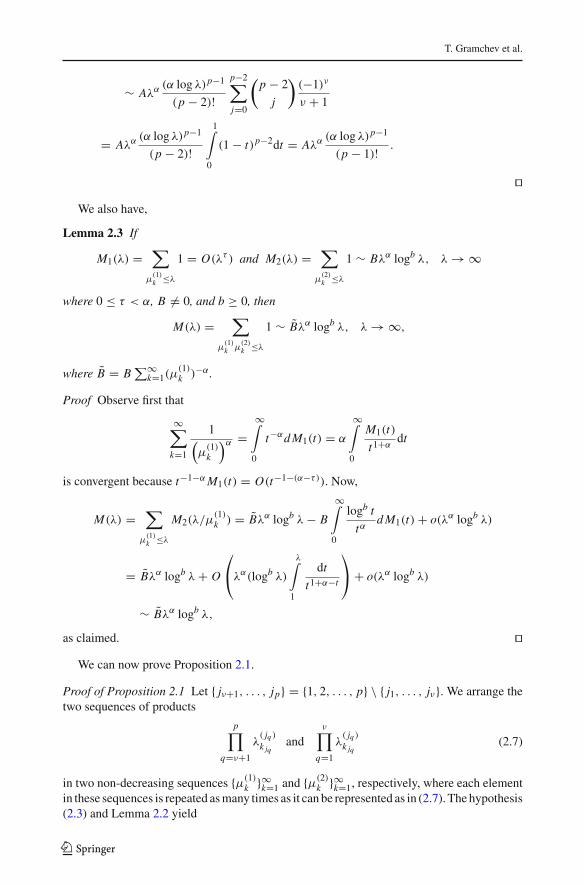
� We also have,
Lemma 2.3 If
M1(λ) =∑
μ(1)k ≤λ
1 = O(λτ ) and M2(λ) =∑
μ(2)k ≤λ
1 ∼ Bλα logb λ, λ → ∞
where 0 ≤ τ < α, B = 0, and b ≥ 0, then
M(λ) =∑
μ(1)k μ
(2)k ≤λ
1 ∼ Bλα logb λ, λ → ∞,
where B = B∑∞
k=1(μ(1)k )−α .
Proof Observe first that
∞∑k=1
1(μ
(1)k
)α =∞∫
0
t−αd M1(t) = α
∞∫
0
M1(t)
t1+αdt
is convergent because t−1−α M1(t) = O(t−1−(α−τ)). Now,
M(λ) =∑
μ(1)k ≤λ
M2(λ/μ(1)k ) = Bλα logb λ − B
∞∫
0
logb t
tαd M1(t) + o(λα logb λ)
= Bλα logb λ + O
⎛⎝λα(logb λ)
λ∫
1
dt
t1+α−t
⎞⎠ + o(λα logb λ)
∼ Bλα logb λ,
as claimed. � We can now prove Proposition 2.1.
Proof of Proposition 2.1 Let { jν+1, . . . , jp} = {1, 2, . . . , p} \ { j1, . . . , jν}. We arrange thetwo sequences of products
p∏q=ν+1
λ( jq )
k jqand
ν∏q=1
λ( jq )
k jq(2.7)
in two non-decreasing sequences {μ(1)k }∞k=1 and {μ(2)
k }∞k=1, respectively, where each elementin these sequences is repeated as many times as it can be represented as in (2.7). The hypothesis(2.3) and Lemma 2.2 yield
123
Weyl asymptotics for tensor products of operators
M2(λ) =∑
μ(2)k ≤λ
1 ∼ Bλα logν−1 λ, λ → ∞,
where B = (αν−1/(ν − 1)!)∏νq=1 A jq . On the other hand, using (2.4), one easily verifies
that
M1(λ) =∑
μ(1)k ≤λ
1 = O(λτ logp−ν λ), λ → ∞.
Applying Lemma 2.3 and noticing that
∞∑k=1
1(μ
(1)k
)α =⎛⎜⎝
∏j /∈{ j1,..., jν }
⎛⎜⎝
∞∑k=1
1(λ
( j)k
)α
⎞⎟⎠
⎞⎟⎠ ,
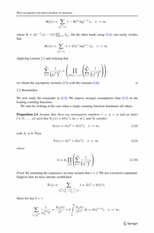
we obtain the asymptotic formula (2.5) with the constant (2.6). � 2.2 Remainders
We now study the remainder in (2.5). We impose stronger assumptions than (2.3) on theleading counting functions.
We start by looking at the case when a single counting function dominates all others.
Proposition 2.4 Assume that there are nonnegative numbers τ < η < α and an indexl ∈ {1, . . . , p} such that N j (λ) = O(λτ ), for j = l, and Nl satisfies
Nl(λ) = Alλα + O(λη), λ → ∞, (2.8)
with Al = 0. Then,
N (λ) = Aλα + O(λη), λ → ∞, (2.9)
where
A = Al
∏j =l
⎛⎜⎝
∞∑k=1
1(λ
( j)k
)α
⎞⎟⎠ . (2.10)
Proof By renaming the sequences, we may assume that l = 1. We use a recursive argument.Suppose that we have already established
N (λ) =∑
λ(1)k1
λ(2)k2
...λ(p−1)k p−1
≤λ
1 = Aλα + O(λη).
Since for any b > τ
∑
λ≤λ(p)k
1
(λ(p)k )b
= Np(λ)
λb+ b
∞∫
λ
Np(t)
tb+1 dt = O(λτ−b), λ → ∞,
123
T. Gramchev et al.
we have
N (λ) =∑
λ(p)k ≤λ
N (λ/λ(p)k )
= Aλα1
( ∞∑k=1
1
(λ(p)k )α
)+ O(λτ ) +
∑
λ(p)k ≤λ
O((λ/λ(p)k )η)
= Aλα1 + O(λτ ) + O(λη),
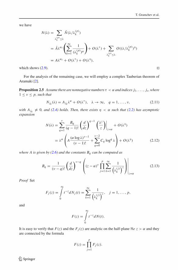
which shows (2.9). � For the analysis of the remaining case, we will employ a complex Tauberian theorem of
Aramaki [2].
Proposition 2.5 Assume there are nonnegative numbers τ < α and indices j1, . . . , jν , where1 ≤ ν ≤ p, such that
N jq (λ) = A jq λα + O(λτ ), λ → ∞, q = 1, . . . , ν, (2.11)
with A jq = 0, and (2.4) holds. Then, there exists η < α such that (2.2) has asymptoticexpansion
N (λ) =ν∑
q=1
Bq
(q − 1)!(
d
dz
)q−1 (λz
z
)∣∣∣∣z=α
+ O(λη)
= λα
⎛⎝A
(α log λ)ν−1
(ν − 1)! +ν−2∑q=0
Cq logq λ
⎞⎠ + O(λη) (2.12)
where A is given by (2.6) and the constants Bq can be computed as
Bq = 1
(ν − q)!(
d
dz
)ν−q
⎛⎜⎝(z − α)ν
p∏j=1
∞∑k=1
1(λ
( j)k
)z
⎞⎟⎠
∣∣∣∣∣∣∣z=α
(2.13)
Proof Set
Fj (z) =∞∫
0
t−zd N j (t) =∞∑
k=1
1(λ
( j)k
)z , j = 1, . . . , p,
and
F(z) =∞∫
0
t−zd N (t).
It is easy to verify that F(z) and the Fj (z) are analytic on the half-plane �e z > α and theyare connected by the formula
F(z) =p∏
j=1
Fj (z).
123
Weyl asymptotics for tensor products of operators
Moreover, Fj (z) is analytic on �e z > τ if j ∈ { j1, . . . , jq}, whereas
Fjq (z) − A jq α
z − α, q = 1, . . . , ν,
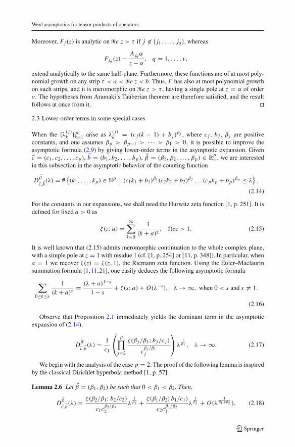
extend analytically to the same half-plane. Furthermore, these functions are of at most poly-nomial growth on any strip τ < a < �e z < b. Thus, F has also at most polynomial growthon such strips, and it is meromorphic on �e z > τ , having a single pole at z = α of orderν. The hypotheses from Aramaki’s Tauberian theorem are therefore satisfied, and the resultfollows at once from it. � 2.3 Lower-order terms in some special cases
When the {λ( j)k }∞k=1 arise as λ
( j)k = (c j (k − 1) + b j )
β j , where c j , b j , β j are positiveconstants, and one assumes βp > βp−1 > · · · > β1 > 0, it is possible to improve theasymptotic formula (2.9) by giving lower-order terms in the asymptotic expansion. Given�c = (c1, c2, . . . , cp), �b = (b1, b2, . . . , bp), �β = (β1, β2, . . . , βp) ∈ R
p+, we are interested
in this subsection in the asymptotic behavior of the counting function
D�β�c,�b(λ) = #
{(k1, . . . , kp) ∈ N
p : (c1k1 + b1)β1(c2k2 + b2)
β2 . . . (cpkp + bp)βp ≤ λ
}.
(2.14)
For the constants in our expansions, we shall need the Hurwitz zeta function [1, p. 251]. It isdefined for fixed a > 0 as
ζ(z; a) =∞∑
k=0
1
(k + a)z, �ez > 1. (2.15)
It is well known that (2.15) admits meromorphic continuation to the whole complex plane,with a simple pole at z = 1 with residue 1 (cf. [1, p. 254] or [11, p. 348]). In particular, whena = 1 we recover ζ(z) = ζ(z, 1), the Riemann zeta function. Using the Euler–Maclaurinsummation formula [1,11,21], one easily deduces the following asymptotic formula
∑0≤k≤λ
1
(k + a)s= (λ + a)1−s
1 − s+ ζ(s; a) + O(λ−s), λ → ∞, when 0 < s and s = 1.
(2.16)
Observe that Proposition 2.1 immediately yields the dominant term in the asymptoticexpansion of (2.14),
D�β�c,�b(λ) ∼ 1
c1
⎛⎝
p∏j=2
ζ(β j/β1; b j/c j )
cβ j /β1j
⎞⎠ λ
1β1 , λ → ∞. (2.17)
We begin with the analysis of the case p = 2. The proof of the following lemma is inspiredby the classical Dirichlet hyperbola method [1, p. 57].
Lemma 2.6 Let �β = (β1, β2) be such that 0 < β1 < β2. Then,
D�β�c,�b(λ) = ζ(β2/β1; b2/c2)
c1cβ2/β12
λ1β1 + ζ(β1/β2; b1/c1)
c2cβ1/β21
λ1β2 + O(λ
1β1+β2 ). (2.18)
123
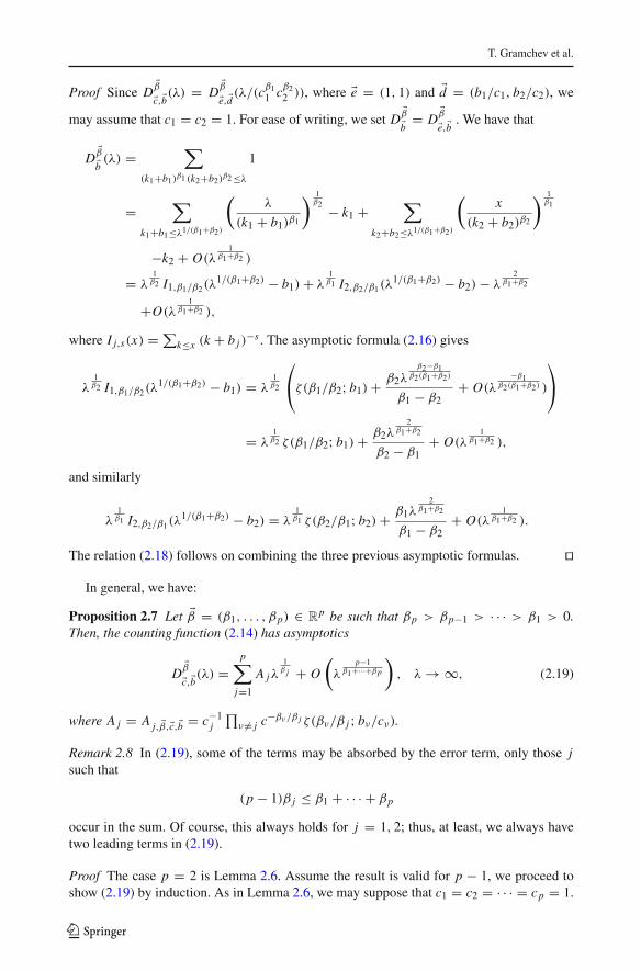
T. Gramchev et al.
Proof Since D�β�c,�b(λ) = D
�β�e, �d(λ/(cβ1
1 cβ22 )), where �e = (1, 1) and �d = (b1/c1, b2/c2), we
may assume that c1 = c2 = 1. For ease of writing, we set D�β�b = D
�β�e,�b . We have that
D�β�b (λ) =
∑
(k1+b1)β1 (k2+b2)β2 ≤λ
1
=∑
k1+b1≤λ1/(β1+β2)
(λ
(k1 + b1)β1
) 1β2 − k1 +
∑
k2+b2≤λ1/(β1+β2)
(x
(k2 + b2)β2
) 1β1
−k2 + O(λ1
β1+β2 )
= λ1β2 I1,β1/β2(λ
1/(β1+β2) − b1) + λ1β1 I2,β2/β1(λ
1/(β1+β2) − b2) − λ2
β1+β2
+O(λ1
β1+β2 ),
where I j,s(x) = ∑k≤x (k + b j )
−s . The asymptotic formula (2.16) gives
λ1β2 I1,β1/β2(λ
1/(β1+β2) − b1) = λ1β2
⎛⎝ζ(β1/β2; b1) + β2λ
β2−β1β2(β1+β2)
β1 − β2+ O(λ
−β1β2(β1+β2) )
⎞⎠
= λ1β2 ζ(β1/β2; b1) + β2λ
2β1+β2
β2 − β1+ O(λ
1β1+β2 ),
and similarly
λ1β1 I2,β2/β1(λ
1/(β1+β2) − b2) = λ1β1 ζ(β2/β1; b2) + β1λ
2β1+β2
β1 − β2+ O(λ
1β1+β2 ).
The relation (2.18) follows on combining the three previous asymptotic formulas. �
In general, we have:
Proposition 2.7 Let �β = (β1, . . . , βp) ∈ Rp be such that βp > βp−1 > · · · > β1 > 0.
Then, the counting function (2.14) has asymptotics
D�β�c,�b(λ) =
p∑j=1
A jλ1
β j + O
(λ
p−1β1+···+βp
), λ → ∞, (2.19)
where A j = A j, �β,�c,�b = c−1j
∏ν = j c−βν/β j ζ(βν/β j ; bν/cν).
Remark 2.8 In (2.19), some of the terms may be absorbed by the error term, only those jsuch that
(p − 1)β j ≤ β1 + · · · + βp
occur in the sum. Of course, this always holds for j = 1, 2; thus, at least, we always havetwo leading terms in (2.19).
Proof The case p = 2 is Lemma 2.6. Assume the result is valid for p − 1, we proceed toshow (2.19) by induction. As in Lemma 2.6, we may suppose that c1 = c2 = · · · = cp = 1.
123
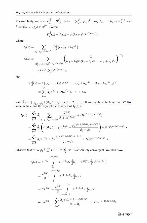
Weyl asymptotics for tensor products of operators
For simplicity, we write D�β�b = D
�β�c,�b . Set α = ∑p
j=2 β j , �d = (b2, b3, . . . , bp) ∈ Rp−1+ , and
�η = (β2, . . . , βp) ∈ Rp−1+ . Write
D�β�b (λ) = I1(λ) + I2(λ) + O(λ1/(α+β1)),
where
I1(λ) =∑
k1+b1≤λ1/(α+β1)
D �η�d(λ/(k1 + b1)
β1),
I2(λ) =∑
∏pj=2(k j +b j )
β j ≤λα/(α+β1)
(λ
(k2 + b2)β2(k3 + b3)β3 . . . (kp + bp)βp
)1/β1
−λ1
α+β1 D �η�d (λα/(α+β1)),
and
D �η�d (λ) = #
{(k2, . . . , kp) ∈ N
p−1 : (k2 + b2)β2 . . . (kp + bp)
βp ≤ λ}
=p∑
j=2
A jλ1
β j + O(λp−2α ), λ → ∞,
with A j = ∏2≤ν,ν = j ζ(βν/β j ; bν) for j = 2, . . . , p. If we combine the latter with (2.16),
we conclude that the asymptotic behavior of I1(λ) is
I1(λ) =p∑
j=2
A j
∑
k+b1≤λ1/(α+β1)
λ1/β j
(k + b1)β1/β j
+ O(λ(p−1)/(α+β1))
=p∑
j=2
A j
(ζ
(β1/β j ; b1
)λ1/β j + β jλ
(α+β j )/(β j (α+β1))
β j − β1
)+ O(λ(p−1)/(α+β1))
=p∑
j=2
A jλ1/β j + A j
β jλ(α+β j )/(β j (α+β1))
β j − β1+ O(λ(p−1)/(α+β1)).
Observe that C := β−11
∫ ∞0 t−1−1/β1 D �η
�d (t)dt is absolutely convergent. We then have
I2(λ) = λ1/β1
λα/(α+β1)∫
0
t−1/β1 d D �η�d (t) − λ
1α+β1 D �η
�d (λα/(α+β1))
= λ1/β1
β1
λα/(α+β1)∫
0
t−1−1/β1 D �η�d (t)dt
= Cλ1/β1 − λ1/β1
β1
∞∫
λα/(α+β1)
t−1−1/β1 D �η�d (t)dt
= Cλ1/β1 −p∑
j=2
A jβ jλ(α+β j )/(β j (α+β1))
β j − β1+ O(λ(p−1)/(α+β1)).
123
T. Gramchev et al.
Thus, we have shown (2.19) except for C = ∏pν=2 ζ(βν/β1; bν). But this fact follows by
comparison with (2.17). The proof is complete. � Remark 2.9 In connection with Proposition 2.7, Estrada and Kanwal have given an interestingdistributional treatment of the asymptotic expansions of type (2.19), which often leads toimprovements in the error term when interpreted in the distributional sense (cf. [11, Sec.5.3]).
3 Counting functions for tensor products of pseudo-differential operators
We now apply results from Sect. 2 to the spectral asymptotics of the tensor products ofpseudo-differential operators and their perturbations. We shall mainly refer to operators inthe Euclidean setting. Parallel results for operators on compact manifold will be outlined atthe end. For the sake of completeness, we begin with a short survey of the classes of Shubin,cf. [7,17,25,31].
3.1 Globally elliptic pseudo-differential operators
Write z = (x, ξ) ∈ R2n and < z >= (1 + |z|2)1/2 = (1 + |x |2 + |ξ |2)1/2. One defines
the class of symbols �mρ (Rn), m ∈ R, 0 < ρ ≤ 1, as the set of all functions a ∈ C∞(R2n)
satisfying, for all γ,
|∂γz a(z)| ≤ Cγ < z >m−ρ|γ |, z ∈ R
2n, (3.1)
with constants independent of z. The corresponding pseudo-differential operator is definedby Weyl quantization as
Pu(x) = awu(x) = 1
(2π)n
∫ei(x−y)ξ a
(x + y
2, ξ
)u(y)dydξ. (3.2)
Note that if the symbol a is a polynomial in the ξ variables, i.e., P in (3.2) is a partialdifferential operator, then the estimates (3.1) force a(z) to be a polynomial in the x−variablesas well, i.e., P is a partial differential operator with polynomial coefficients.
Let us introduce the global Sobolev spaces Hs(Rn), s ∈ N, Hilbert spaces with the norm
||u||s =∑
|α|+|β|≤s
||xα Dβu|| < ∞. (3.3)
By interpolation and duality the definition extends to s ∈ R, and we have⋂
s Hs(Rn) =S(Rn),
⋃s Hs(Rn) = S ′(Rn). The immersion ι :s Hs → Ht is compact for s > t . If
a ∈ �mρ (Rn), then aw : Hs(Rn) → Hs−m(Rn) continuously for every s ∈ R, hence
aw : S(Rn) → S(Rn), S ′(Rn) → S ′(Rn). In the following we shall assume that for large|z|,
a(z) = am(z) + am−ρ(z), (3.4)
where am(t z) = tmam(z), t > 0. We then say that a is globally elliptic if
am(z) = 0 for z = 0. (3.5)
Operators with globally elliptic symbol possess parametrix. Namely, there exists b ∈�−m
ρ (Rn) such that awbw = I + R1 and bwaw = I + R2, where R1, R2 : S ′(Rn) → S(Rn).It follows that aw : Hs(Rn) → Hs−m(Rn) is a Fredholm operator and then eigenfunctions,
123
Weyl asymptotics for tensor products of operators
i.e., solutions of awu = 0, do not depend on s ∈ R and belong to S(Rn). Passing now tospectral theory, we assume that a ∈ �m
ρ (Rn), m > 0, is real-valued and globally elliptic witham(z) > 0, for z = 0. Then P = awu : Hm(Rn) �→ L2(Rn) is self-adjoint. The resolventis compact and the spectrum is given by a sequence of real eigenvalues λk → ∞ with finitemultiplicity; the eigenfunctions belong to S(R) and form an orthonormal basis. The spectralcounting function NP (λ) = #{k : λk ≤ λ} behaves as
NP (λ) = Aλ2n/m + O(λσ ), λ → ∞, (3.6)
for some σ < 2n/m, with
A = 1
(2π)n
∫
am (z)≤1
dz. (3.7)
A sharp form of the remainder in (3.6) can be obtained when a ∈ �m(Rn) = �m1 (Rn) admits
an asymptotic expansion in homogeneous terms a ∼ ∑k∈N
am−2k . Then, with A as before,
NP (λ) = Aλ2n/m + O(λ2(n−1)/m), (3.8)
see, for example, Helffer [17, p. 175]. In the sequel, we shall assume that P is strictly positive,so that 0 < λ1 ≤ λ2 ≤ . . .. For P as before, we may define the complex powers Pz, z ∈ C.They are trace class operators if �ez < −2n/m, and, by analytic continuation, we definethe zeta function associated with P as
ζP (z) = Tr(P−z) =∞∑
k=1
λ−zk . (3.9)
3.2 Spectral asymptotics for tensor products
To give a precise functional frame to the results in the sequel, we shall introduce firstthe tensorized global Sobolev spaces. Write now x j , y j ∈ R
n j , z j = (x j , y j ) ∈ R2n j ,
j = 1, . . . , p, n = n1 + · · · + n p , x = (x1, . . . , x p), y = (y1, . . . , yp) ∈ Rp ,
z = (z1, . . . , z p) = (x1, y1, . . . , x p, yp). For �s = (s1, . . . , sp) ∈ Rp , we define the ten-
sor product of Hilbert spaces
H �s(Rn) =p⊗
j=1
Hs j (Rn j ). (3.10)
When the components of �s are nonnegative integers, from (3.3) we recapture as norm
||u||�s =∑
|α j |+|β j |≤s j
j=1,...,p
||xα1 . . . xα2 Dβ1x1
. . . Dβpx p u||. (3.11)
We have⋂
�s H �s(Rn) = S(Rn) and⋃
�s H �s(Rn) = S ′(Rn). The immersion ι : H �s(Rn) →H �t (Rn) is compact if �s > �t, i.e., s j > t j for j = 1, . . . , p.
As announced at the Introduction, we consider now Pj = awj in R
n j , j = 1, . . . , p, withreal-valued symbol a j ∈ �m j (Rn j ), m j > 0,, and am j (z) > 0 for z = 0 in (3.5); we furtherdefine
P = P1 ⊗ · · · ⊗ Pp, (3.12)
123
T. Gramchev et al.
as operator P : H �s(Rn) → H �s− �m(Rn), �m = (m1, . . . , m p), for every �s ∈ Rp . In particular,
we have P : H �m(Rn) → L2(Rn) and P : S(Rn) → S(Rn), S ′(Rn) → S ′(Rn). Moreover,P is self-adjoint and strictly positive, if the factors Pj are assumed to be strictly positive.
If we denote by {λ( j)k }∞k=1 the eigenvalues of Pj , according to the Introduction, the eigen-
values of P are of the form λ(1)k1
. . . λ(p)kp
, and the eigenfunctions are tensor products of therespective eigenfunctions; hence, they belong to S(Rn).
It is worth observing that P can be written in the pseudo-differential form (3.2) with symbola(z) = a1(z1) . . . ap(z p). However, the estimate (3.1) fails in general, and the considerationsof Sect. 3.1 do not apply in this context. For the case p = 2, we address to [5], cf. [6,26],where a calculus was achieved in terms of vector-valued symbols. Here, to find an asymptoticexpansion for NP (λ), we shall use (1.2) in combination with the analysis of Sect. 2. In fact,from (3.6) and (3.7), we have
NPj ∼ A jλ2n j /m j with A j = 1
(2π)n j
∫
am j (z j )≤1
dz j . (3.13)
Writing ζPj for the zeta function of Pj , we immediately obtain from Proposition 2.1:
Theorem 3.1 Let P = P1 ⊗ · · · ⊗ Pp be as above and let α = max j {2n j/m j }. Let furtherj1, . . . , jν be the indices such that α = 2n jq /m jq , q = 1, . . . , ν. Then, P has spectralasymptotics
NP (λ) =∑
λ(1)k1
λ(2)k2
...λ(p)k p
≤λ
1 ∼⎛⎝
ν∏q=1
A jq ·∏
j /∈{ j1,..., jq}ζPj (α)
⎞⎠ λα (α log λ)ν−1
(ν − 1)! , λ → ∞,
(3.14)
where A j is given by (3.13).
We remark that the case p = 2, ν = 1 or ν = 2, of Theorem 3.1 also follows from theresults of [6], see also [5]).
As far as the reminder in (3.14) concerns, from (3.6) and Proposition 2.5, we obtain
NP (λ) = λαν−1∑q=0
Cq logq λ + O(λη), (3.15)
for some η < α. The coefficient Cν−1 is given by (3.14) and the other constants Cq , q =0, . . . , ν − 2, are determined by (2.12), (2.13), and the values of the derivatives or poles ofthe zeta functions ζPj (z) at z = α, j = 1, . . . , p.
Willing sharp values of η in the remainder, we further assume that a j ∈ �m j (Rn j ) witha j ∼ ∑
k∈Nam j −2k and we use (3.8). Proposition 2.4 yields,
Theorem 3.2 Let P = P1⊗· · ·⊗Pp be as above. Assume that there is an index l ∈ {1, . . . , p}such that 2nl/ml > β = max j =l{2n j/m j }. Then
NP (λ) =⎛⎝Al
∏j =l
ζPj (α)
⎞⎠ λ
2nlml + O(λη), (3.16)
for any η with η > max{β, 2(nl − 1)/ml}.
123
Weyl asymptotics for tensor products of operators
The following example shows that the exponent η = β is sharp in (3.16).
Example 3.3 (Tensorized Hermite operators). For tensor products of Hermite operators it ispossible to detect lower-order terms in the asymptotic expansion (3.16). Namely, let us fix�β = (β1, . . . , βp) with β1 < · · · < βp, �c = (c1, . . . , cp), �b = (b1, . . . , bp), p-tuples ofpositive real numbers, cf. Sect. 2.3, and consider
Hj,c j ,b j = c j
2(−∂2
x j+ x2
j ) − c j
2+ b j , j = 1, . . . , p, (3.17)
so that for c j = 1, b j = 1, we recapture Hj in (1.3) of the Introduction. The eigenvalues of
Hj,c j ,b j , as one- dimensional operator, are λ( j)k = c j (k − 1) + b j , k = 1, 2, . . .. We then
define the tensorized Hermite operator
H�β�c,�b =
p⊗j=1
Hβ jj,c j ,b j
. (3.18)
By Proposition 2.7, we have for the corresponding counting function
N (λ) = D�β�c,�b(λ) =
p∑j=1
A jλ1/β j + O
(λ
p−1β1+···+βp
)(3.19)
with A j as in Proposition 2.7. In particular, for p = 2, c j = 1, b j = 1, j = 1, 2, we obtain(1.8) of the Introduction.
3.3 Asymptotics for lower-order perturbations
For simplicity, we shall assume that the factors Pj in P = P1⊗· · ·⊗Pp are partial differentialoperators with polynomial coefficients:
Pj =∑
|α j |+|β j |≤m j
c( j)α j ,β j
xα j Dβ jx j , x j ∈ R
n j . (3.20)
As before, we assume that Pj is elliptic, with principal symbol
p( j)m j (x, ξ) =
∑|α j |+|β j |=m j
c( j)α j ,β j
xα jj ξ
β jj > 0 for (x j , ξ j ) = (0, 0), (3.21)
self-adjoint and strictly positive, j = 1, . . . , p. We shall study
A = P + R, (3.22)
where R is a partial differential operator with polynomial coefficients having lower orderwith respect to P , in the sense that, writing �α = (α1, . . . , αp), �β = (β1, . . . , βp) ∈ N
n, n =n1 + · · · + n p ,
R =∑
|α j |+|β j |<m j
j=1,...,p
cαβ x �α D�β . (3.23)
Note that each term of the sum in (3.23) can be regarded as a tensor product:
x �α D�β = xα1
1 Dβ1x1
⊗ · · · ⊗ xαpp D
βpx p ,
123
T. Gramchev et al.
hence, for every �s ∈ Rp ,
A = P + R : H �s(Rn) → H �s− �m(Rn).
We shall first construct a parametrix for A. In absence of symbolic calculus, we shall use inthe proof a direct argument.
Proposition 3.4 For every fixed integer M > 0, we can find B : H �s(Rn) → H �s+ �m(Rn)
for every �s = (s1, . . . , sp) ∈ Rp, such that B A = I + S′, AB = I + S′′, where S′, S′′ :
H �s(Rn) → H �s+ �M (Rn), with �M = (M, . . . , M).
Proof Consider
P−1 = P−11 ⊗ · · · ⊗ P−1
p : H �s(Rn) → H �s+ �m(Rn).
We have P−1 A = P−1(P + R) = I − S with
S = −P−1 R : H �s(Rn) → H �s+�1(Rn).
Define then
B =M−1∑j=0
S j P−1 : H �s(Rn) → H �s+ �M (Rn).
We have
B A =M−1∑j=0
S j (I − S) = I − SM ,
where S′ = −SM : H �s(Rn) → H �s+ �M (Rn). It is easy to check that B is also a rightparametrix. �
Corollary 3.5 The solution u ∈ S ′(Rn) of Au = f ∈ S(Rn) belongs to S(Rn).
Proof If u ∈ S ′(Rn), then u ∈ H �s(Rn) for some �s. Taking B as in Proposition 3.4, we obtain
B Au = (I + S′)u = B f,
hence, u = B f − S′u. We have B f ∈ S(Rn) and S′u ∈ H �s+ �M (Rn). Since M in Proposition3.4 can be fixed as large as we want, we conclude u ∈ S(Rn). �
Corollary 3.6 The operator A : H �s(Rn) → H �s− �m(Rn) is Fredholm, for every fixed �s ∈ Rn.
Proof Let us apply Proposition 3.4 with M = 1. Since the inclusion H �s+�1(Rn) → H �s(Rn)
is compact, the Fredholm property is proved. �
Let us assume now that the operator A in (3.22) is self-adjoint. It follows from the precedingarguments that the resolvent is compact and the eigenfunctions belong to S(Rn). Assumefurther that A is strictly positive; we write 0 < λ1 ≤ λ2 ≤ ... for its eigenvalues and NA forits spectral counting function. We give below an asymptotic formula for λk . In the sequel wewrite f � g to mean that f = O(g) and g = O( f ) are both valid.
123
Weyl asymptotics for tensor products of operators
Theorem 3.7 Let A = P + R in (3.22) be as above. We use for P the notation of Theorem3.1, namely we write α = max j {2n j/m j } and we assume that α = 2n j/m j for ν indices.We then have
λk � k1/α(log k)−(ν−1)/α, k → ∞ (3.24)
and
NA(λ) � λα logν−1 λ, λ → ∞. (3.25)
Proof We have
||Au||2 = ||AP−1 Pu||2 ≤ C1||Pu||2 with C1 = ||AP−1||2L(L2).
On the other hand, using Proposition 3.4, we may write I = B A − S′ and thus,
||Pu||2 = ||P(B A − S′)u||2 ≤ 2||P B Au||2 + 2||P S′u||2| ≤ C2(||Au||2 + ||u||2)with
C2 = 2 max{||P B||2L(L2), ||P S′||2L(L2)
},where ||P S′||L(L2) < ∞ if M in Proposition 3.4 is chosen sufficiently large. We now rewritethe preceding estimates as
(A2u, u) ≤ (C1 P2u, u) and (P2u, u) ≤ (C2(A2 + I )u, u).
Using the classical max-min formula for the eigenvalues of A2, P2 and denoting here μk theeigenvalues of P , we deduce
λ2k ≤ C1μ
2k and μ2
k ≤ C2(λ2k + 1).
Hence, λk � μk . As a final step in the proof, we apply the following lemma.
Lemma 3.8 If the sequence 0 < μ1 ≤ μ2 ≤ . . ., μk → ∞, admits counting function
N (μ) ∼ rμα logs μ, μ → ∞,
with r, α > 0 and s ≥ 0, then
μk ∼(α
r
)1/α
k1/α(log k)−s/α, k → ∞. (3.26)
The proof of this lemma is a simple combination of Proposition 4.6.4, page 198, andLemma 5.2.9, page 219, from [25], and it is therefore omitted. Since for the counting functionNP (μ), we have from Theorem 3.1
NP (μ) ∼ rμα(log μ)ν−1
for a constant r , we deduce from Lemma 3.8 for the eigenvalues μk of P the asymptotics(3.26) with s = ν − 1. Hence, (3.24) follows. The asymptotic formula (3.25) can be easilydeduced from (3.24), we leave details to the reader. �
The rough asymptotics (3.25) can hopefully be improved, as suggested by the result from[6], which gives NA(λ) ∼ NP (λ) in the case p = 2. Furthermore, we expect formula (3.15)is invariant under lower-order perturbations. On the contrary, the precise asymptotics (3.19)for tensorized Hermite operators should be lost, after addition of lower-order terms.
123
T. Gramchev et al.
3.4 Pseudo-differential operators on closed manifolds
We now look at pseudo-differential operators on closed manifolds. Let M1, M2, . . . , Mp beclosed manifolds with dim M j = n j . We consider elliptic self-adjoint pseudo-differentialoperators Pj on M j of order m j and principal symbol am j (x j , ξ j ) > 0 for (x j , ξ j ) ∈T ∗M j \ (M j × {0}), j = 1, . . . , p. We denote by dx j dξ j the natural volume form onthe cotangent bundle T ∗M j . Under these circumstances, Hörmander’s theorem [31, Chap.III] gives us the asymptotic behavior of each counting function NPj (λ) of the eigenvalues
{λ( j)k }∞k=1 of Pj . In fact,
NPj (λ) =∑
λ( j)k ≤λ
1 = A jλn j /m j + O(λ(n j −1)/m j ), λ → ∞,
where
A j = 1
(2π)n j
∫
am j (x j ,ξ j )<1
dx j dξ j , j = 1, . . . , p. (3.27)
As usual, ζPj denotes the zeta function of the operator Pj .Proposition 2.4 directly gives the spectral asymptotics of the operator P = P1 ⊗ P2 ⊗
· · · ⊗ Pp on the closed manifold M = M1 × M2 × · · · × Mp of dimension dim M = n =n1 + n2 + · · · + n p , whenever one of the counting functions NPl dominates all the others.
Theorem 3.9 Let Pj be elliptic self-adjoint strictly positive pseudo-differential operator asabove, j = 1, . . . , p,. Suppose that there is l ∈ {1, 2, . . . , p} such that nl/ml > n j/m j forall j = l. Then, the spectral counting function NP of the operator P = P1 ⊗ P2 ⊗ · · · ⊗ Pp
has asymptotics
NP (λ)=∑
λ(1)k1
λ(2)k2
...λ(p)k p
≤λ
1=⎛⎝Al
∏j =l
ζPj (nl/ml)
⎞⎠ λnl/ml +O(λτ ), λ → ∞, (3.28)
where Al is given by (3.27) and τ satisfies max{(nl − 1)/ml , max j =l n j/m j } < τ < nl/ml.
For the special case of the tensor product of two elliptic operators with one countingfunction dominating the other one, the error term in (3.2) improves that from [5, Thrm. 3.2 ]for bisingular operators.
We leave to the reader statements and proofs for the counterparts of Theorem 3.1, (3.15)and Theorem 3.7 in the setting of closed manifolds.
References
1. Apostol, T.M.: Introduction to Analytic Number Theory. Springer, NY (1976)2. Aramaki, J.: On an extension of the Ikehara Tauberian theorem. Pac. J. Math. 133, 13–30 (1988)3. Arnold, V.I.: Lectures on partial differential equations. Springer, Publishing House PHASIS, Berlin,
Moscow (2004)4. Atiyah, M.F., Singer, I.M.: The index of elliptic operators: I. Ann. Math. 87(3), 484–530 (1968)5. Battisti, U.: Weyl asymptotics of bisingular operators and Dirichlet divisor problem. Math. Z. 272, 1365–
1381 (2012)6. Battisti, U., Gramchev, T., Pilipovic, S., Rodino, L.: Globally bisingular elliptic operators. In: Opera-
tor Theory, Pseudo-Differential Equations and Mathematical Physics, Operator Theory: Advances andApplications. Birkhäuser, Basel (2012)
123
Weyl asymptotics for tensor products of operators
7. Boggiatto, P., Buzano, E., Rodino, L.: Global Hypoellipticity and Spectral Theory. Math. Res. 92.Akademie, Berlin (1996)
8. Brown, A., Pearcy, C.: Spectra of tensor products of operators. Proc. Amer. Math. Soc. 17, 162–166(1966)
9. Brüning, J., Guillemin, V. (eds.): Fourier Integral Operators. Springer, Berlin (1994)10. Coriasco, S., Manicia, L.: On the spectral asymptotics of operators on manifolds with ends. Abstr. Appl.
Anal. 2013, Article ID 909782, 21 pp11. Estrada, R., Kanwal, R.P.: A Distributional Approach to Asymptotics. Theory and Applications, 2nd edn.
Birkhäuser, Boston, MA (2002)12. Götze, F.: Lattice point problems and values of quadratic forms. Invent. Math. 157, 195–226 (2004)13. Gramchev, T., Pilipovic, S., Rodino, L.: Classes of degenerate elliptic operators in Gelfand-Shilov spaces.
In: New Developments in Pseudo-Differential Operators Operator Theory: Advances and Applications,vol. 189, pp. 15–31 (2009)
14. Gramchev, T., Pilipovic, S., Rodino, L., Wong, M.W.: Spectral properties of the twisted bi-Laplacian.Arch. Math. (Basel) 93, 565–575 (2009)
15. Gramchev, T., Pilipovic, S., Rodino, L., Wong, M.W.: Spectral of polynomials of the twisted Laplacian.Atti Acc. Scienze, Torino, Cl. Sc. FMN 144, 145–154 (2010)
16. Hardy, G.H.: On Dirichlet’s divisor problem. Proc. Lond. Math. Soc. (2) 15, 1–25 (1916)17. Helffer, B.: Théorie spectrale pour des opérateurs globalement elliptiques, Astérisque 112. Société Math-
ématique de France, Paris (1984)18. Hill, R., Parnovski, L.: The variance of the hyperbolic lattice point counting function. Russ. J. Math. Phys.
12, 472–482 (2005)19. Hörmander, L.: The spectral function of an elliptic operator. Acta Math. 121, 173–218 (1968)20. Huxley, M.N.: Exponential sums and lattice points. III. Proc. Lond. Math. Soc. (3) 87, 591–609 (2003)21. Ivic, A.: The Riemann Zeta-Function. Theory and Applications. Dover Publications, New York (2003)22. Kaplitskiı, V.M.: On the asymptotic distribution of the eigenvalues of a second-order self-adjoint hyper-
bolic differential operator on a two-dimensional torus. Sib. Math. J. 51, 830–846 (2010)23. Kamotski, I., Ruzhansky, M.: Regularity properties, representation of solutions, and spectral asymptotics
of systems with multiplicities. Commun. Partial Differ. Equ. 32, 1–35 (2007)24. Melrose, R., Rochou, F.: Index in K-theory for families of fibred cusp operators. K-theory 37, 25–104
(2006)25. Nicola, F., Rodino, L.: Global Pseudo-Differential Calculus on Euclidean Spaces. Birkhäuser, Basel
(2010)26. Nicola, F., Rodino, L.: Residues and index for bisingular operators. In: C+−algebras and elliptic theory,
pp. 187–202. Trends in Mathematics, Birkhäuser, Basel (2006)27. Rodino, L.: Polysingular integral operators. Ann. Math. Pura Appl. 124, 59–106 (1980)28. Schecter, M.: On the spectra of operators on tensor products. J. Funct. Anal. 4, 95–99 (1969)29. Schulze, B.-W.: Pseudo-differential calculus on manifolds with geometric singularities, pp. 37–83. Fields
Inst. Commun., 52, Amer. Math. Soc., Providence, RI (2007)30. Shulze, B.-W.: The iterative structure of the corner calculus. In: Pseudo-Differential Operators: Analysis,
Applications and Computations, Operator Theory: Advances and Applications, 213. Birkhäuser, Basel(2011)
31. Shubin, M.: Pseudodifferential Operators and Spectral Theory. Springer, Berlin (1987)32. Stein, E., Shakarchi, R.: Functional Analysis. Introduction to Further Topics in Analysis. Princeton Uni-
versity Press, Princeton, NJ (2011)33. Wong, M.W.: Weyl transforms and a degenerate elliptic partial differential equation. Proc. R. Soc. Lond.
Ser. A Math. Phys. Eng. Sci. 461, 3863–3870 (2005)
123
![ELEMENTARY DIVISORS AND MODULES · 1949] ELEMENTARY DIVISORS AND MODULES 467 Theorem 3.1. Let R be a ring satisfying the following conditions: (1) all divisors of 0 are in the radical,](https://img.pdfslide.us/doc/110x75/5f6102e3756044250833a043/elementary-divisors-and-1949-elementary-divisors-and-modules-467-theorem-31-let.jpg)
![· 2013-10-08 · arXiv:0710.0126v1 [math.AP] 1 Oct 2007 REDUCED WEYL ASYMPTOTICS FOR PSEUDODIFFERENTIAL OPERATORS ON BOUNDED DOMAINS II THE COMPACT GROUP CASE ROCH CASSANAS AND](https://img.pdfslide.us/doc/110x75/5f0b560e7e708231d4300318/ramacherpreprint-2013-10-08-arxiv07100126v1-mathap-1-oct-2007-reduced.jpg)


![Weyl points in photonic-crystal superlatticessoljacic/Weyl-points_2DMat.pdf · of Weyl points have been reported in a three-dimensional double-gyroid photonic crystal [45] and in](https://img.pdfslide.us/doc/110x75/5ec846dbd0cd7c3a730fb4cc/weyl-points-in-photonic-crystal-soljacicweyl-points2dmatpdf-of-weyl-points.jpg)