DISCUSSION PAPER SERIES NO. 2019-16

DECEMBER 2019

Welfare Impacts of Rice Tariffication

Roehlano M. Briones

The PIDS Discussion Paper Series constitutes studies that are preliminary and subject to further revisions. They are being circulated in a limited number of copies only for purposes of soliciting comments and suggestions for further refinements. The studies under the Series are unedited and unreviewed. The views and opinions expressed are those of the author(s) and do not necessarily reflect those of the Institute. Not for quotation without permission from the author(s) and the Institute.

CONTACT US:RESEARCH INFORMATION DEPARTMENTPhilippine Institute for Development Studies

18th Floor, Three Cyberpod Centris - North Tower EDSA corner Quezon Avenue, Quezon City, Philippines

publications@mail.pids.gov.ph(+632) 8877-4000 https://www.pids.gov.ph

Welfare Impacts of Rice Tariffication

Roehlano M. Briones

PHILIPPINE INSITITUTE FOR DEVELOPMENT STUDIES

December 2019

2

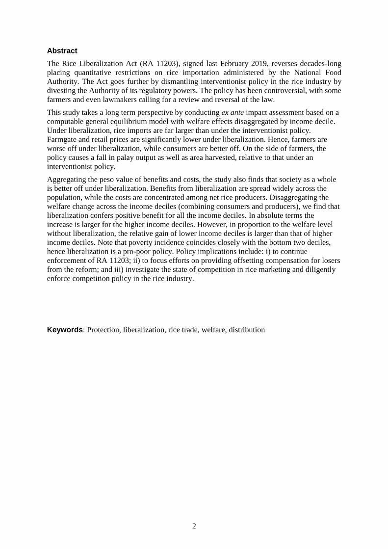
Abstract

The Rice Liberalization Act (RA 11203), signed last February 2019, reverses decades-long

placing quantitative restrictions on rice importation administered by the National Food

Authority. The Act goes further by dismantling interventionist policy in the rice industry by

divesting the Authority of its regulatory powers. The policy has been controversial, with some

farmers and even lawmakers calling for a review and reversal of the law.

This study takes a long term perspective by conducting ex ante impact assessment based on a

computable general equilibrium model with welfare effects disaggregated by income decile.

Under liberalization, rice imports are far larger than under the interventionist policy.

Farmgate and retail prices are significantly lower under liberalization. Hence, farmers are

worse off under liberalization, while consumers are better off. On the side of farmers, the

policy causes a fall in palay output as well as area harvested, relative to that under an

interventionist policy.

Aggregating the peso value of benefits and costs, the study also finds that society as a whole

is better off under liberalization. Benefits from liberalization are spread widely across the

population, while the costs are concentrated among net rice producers. Disaggregating the

welfare change across the income deciles (combining consumers and producers), we find that

liberalization confers positive benefit for all the income deciles. In absolute terms the

increase is larger for the higher income deciles. However, in proportion to the welfare level

without liberalization, the relative gain of lower income deciles is larger than that of higher

income deciles. Note that poverty incidence coincides closely with the bottom two deciles,

hence liberalization is a pro-poor policy. Policy implications include: i) to continue

enforcement of RA 11203; ii) to focus efforts on providing offsetting compensation for losers

from the reform; and iii) investigate the state of competition in rice marketing and diligently

enforce competition policy in the rice industry.

Keywords: Protection, liberalization, rice trade, welfare, distribution

3

Table of Contents

1. Introduction .......................................................................................................... 5

2. Implementation of RA 11203 and its immediate aftermath .................................. 6

Context ................................................................................................................................... 6

The reform ............................................................................................................................. 7

Immediate aftermath of rice tariffication ............................................................................... 8

3. Related Studies on Tariffication ......................................................................... 13

4. Methodology ...................................................................................................... 14

AMPLE-CGE Base model ................................................................................................... 14

Extensions to the AMPLE-CGE .......................................................................................... 15

Welfare estimation ............................................................................................................... 17

Set-up of scenarios ............................................................................................................... 18

5. Results ............................................................................................................... 19

Imports ................................................................................................................................. 19

Palay production and area harvested.................................................................................... 19

Farmgate and retail price ..................................................................................................... 20

Welfare ................................................................................................................................. 21

6. Conclusion ......................................................................................................... 24

Summary of results .............................................................................................................. 24

Limitations of the analysis ................................................................................................... 25

Implications.......................................................................................................................... 25

Bibliography ............................................................................................................. 26

4

List of Figures

Figure 1: Nominal Protection Rate for rice (%) ......................................................................... 7

Figure 2: Annual and monthly price of Vietnam White Rice, in USD per ton, 2017 - 2019 .. 10

Figure 3: Two-year, same-month average of monthly prices, Philippines, 2016-2017, Php per

kg.............................................................................................................................................. 11

Figure 4: Monthly rice prices, 2018, in Php per kg ................................................................. 11

Figure 5: Indicators for monthly farmgate price, June 2014 – June 2015 ............................... 12

Figure 6: Monthly retail price, level and coefficient of variation (three-month average), June

2014 – June 2015 ..................................................................................................................... 12

Figure 7: Rice import growth projections by scenario, 2019 – 2030 (%) ................................ 19

Figure 8: Rice production growth projections, by scenario, 2019 – 2030 (%) ........................ 20

Figure 9: Rice area harvested growth projections, by scenario, 2019 – 2030 (%) .................. 20

Figure 10: Growth projections for rice farmgate price, by scenario, 2019 – 2030 (%) ........... 21

Figure 11: Growth projections for rice retail price, by scenario, 2019 – 2030 (%) ................. 21

Figure 12: Growth projections for rice farmers’ income, by scenario, 2019 – 2030 (%) ........ 21

Figure 13: Decline in farmers’ income due to liberalization as a percentage of reference

income, 2019-2030 .................................................................................................................. 23

Figure 14: Present value of social welfare increase from liberalization, by decile, 2019 – 2030

(Php millions in 2016 prices) ................................................................................................... 24

List of Tables

Table 1: Weekly prices of rice in Php per kg, September 2019 ................................................ 8

Table 2: Prices (Php per unit) and expenditure shares by decile, Philippines, 2015 ............... 16

Table 3: Prices (Php per unit) and expenditure elasticities by decile, Philippines, 2015 ........ 17

Table 4: Prices (Php per unit) and own-price elasticities by per capita income decile,

Philippines, 2015...................................................................................................................... 17

Table 5: Impact on rice farmers’ income by decile, 2019 – 2030 (Php millions, fixed 2016

prices) ....................................................................................................................................... 22

Table 6: Equivalent variation by decile, 2019 – 2030 (Php millions, fixed 2016 prices) ....... 23

5

Welfare impacts of tariffication

Roehlano M. Briones*

1. Introduction

The Rice Liberalization Act (RA 11203), signed only last February 2019, reverses decades-

long placing quantitative restrictions (QRs) on rice importation administered by the National

Food Authority (NFA), which had aimed to shield the local rice industry from foreign

competition. The Act goes further by dismantling the interventionist policy in the domestic rice

industry by divesting NFA of its regulatory powers.

The sole non-tariff barrier permitted in rice importation is the application of sanitary and

phytosanitary standards (SPS), which is the same import regime applied to all other agricultural

among all World Trade Organisation (WTO) member states. There remains however a tariff

barrier in the form of a customs duty of 35 percent or higher. The Act also provides a safety

net for rice farmers using a Rice Competitiveness Enhancement Fund or Rice Fund, to be

funded by in part by tariff escalation.

RA 11203 has already been blamed for adverse impacts on palay farmers owing to a decline in

palay prices. Policymakers are keen to find out whether the policy has had unacceptably high

cost, compared with offsetting benefits to consumers. Findings of the study will inform

legislators in considering the merits of the law, as well as provide inputs for implementing

safety net programs for affected farmers.

In evaluating the policy, a key consideration is the time horizon. The adverse impacts that

have been observed are certainly of short-run character as the implementation of the law is

very recent. Policy evaluation should also pay careful attention to the long run. This will

require ex ante assessment of future impacts of rice industry liberalization.

The general aim of this paper is to provide these ex ante estimates of welfare impact and

examine how this impact is distributed across household groups. Specifically, the study aims

to:

1. Describe the implementation of RA 11203 thus far and its immediate aftermath;

2. Generate long term projections of the impact of rice industry liberalization on market

outcomes, namely output, area harvested, and prices, especially at the farmgate and

retail levels;

3. Provide ex ante estimates of the welfare and distributional impact of market

outcomes, up to the level of the household per capita income decile.

Ex ante impact estimates will be generated from an extended version of the Agricultural

Market Model for Policy Evaluation Computable General Equilibrium (AMPLE-CGE)

Model, a public domain CGE model previously described by Briones (2018). The extension

takes the form of disaggregation of the households in the model into income deciles,

calibrated from the Family Income and Expenditures Survey (FIES) data.

* Research Fellow, Philippine Institute for Development Studies

6

2. Implementation of RA 11203 and its immediate aftermath

Context

Prior to RA 11203, government had been intervening actively in the rice industry through the

actions and restrictions imposed by the NFA. Founded in 1972 (then as the National Grains

Authority), the agency had the following functions, among others:

• Controlling imports by a system of import licensing and QRs;

• Regulating and monitoring players in rice marketing and postharvest operations;

• Purchasing palay (and corn) grains and maintaining a buffer stock;

• Distributing milled rice to support government’s calamity response as well as its

poverty alleviation program.

On the other hand, government acceded to the WTO in 1995 and committed to opening up its

agricultural trade. In particular, it enacted RA 8178, the Agricultural Tariffication Act, by

which it officially abandoned quantitative restrictions, converting these into equivalent tariff

protection – a process known as tariffication. The government agreed to place ceilings on

tariffs; allow a minimum amount of imports per year at a lower tariff rate (the so-called “in-

tariff quota”), known domestically as Minimum Access Volume (MAV);

However, RA 8178 expressly provided an exception in the case of rice, which retained its

status quo policy regime under NFA. The exception was provided a legal cover with respect

to WTO by obtaining a “special treatment” for rice in relation to the WTO Agreement on

Agriculture (AoA). Nonetheless a tariff rate quota was accepted for rice through a 50 percent

binding (which was the actual rate applied both in-quota and out-quota), and a MAV of up to

238,940 tons by 2005. However the special treatment was approved by WTO for only ten

years (up to 2005).

The government applied for an extension of the special treatment, citing lack of readiness of

rice producers to face foreign competition, which was approved to 2012. Government needed

to concede an increase in MAV to 350,000 tons at a tariff rate of 40 percent (without change

in the original ceiling). In a separate negotiation, the government also conceded a special

tariff treatment for ASEAN exporters of only 35 percent under the ASEAN Trade in Goods

Agreement (ATIGA) of 2009 as part of its participation in the ASEAN Free Trade Area

(subsequently subsumed into the ASEAN Economic Community).

Another extension was sought after 2012, which was approved as a waiver running through

to 2017. The government needed to make further concessions, which for rice took the form

an increase in another increase in the MAV to 805,200 tons, at the ATIGA rate of 35 percent.

This access was to be allocated by agreement to various WTO members (the “country-

specific quotas”).

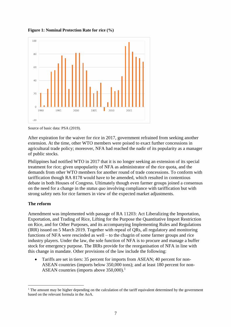
The protection rate conferred by a QR can be measured by the nominal protection rate (NPR).

The NPR or “implicit tariff” can well exceed the protection given by the explicit tariff,

depending on trends in domestic and world prices, and the tightness of import restrictions.

Figure 1 shows the annual NPRs (the percentage excess of wholesale to border price). There

were local peaks in mid-1990s, early 2000s, and 2013-15; the low point was in 2008 when

NPR even turned negative owing to world rice price crisis. Since the mid-1990s, world prices

have trended downward, but domestic prices were insulated from this reduction. After 2000,

the NPR averaged around 90 percent level.

7

Figure 1: Nominal Protection Rate for rice (%)

Source of basic data: PSA (2019).

After expiration for the waiver for rice in 2017, government refrained from seeking another

extension. At the time, other WTO members were poised to exact further concessions in

agricultural trade policy; moreover, NFA had reached the nadir of its popularity as a manager

of public stocks.

Philippines had notified WTO in 2017 that it is no longer seeking an extension of its special

treatment for rice; given unpopularity of NFA as administrator of the rice quota, and the

demands from other WTO members for another round of trade concessions. To conform with

tariffication though RA 8178 would have to be amended, which resulted in contentious

debate in both Houses of Congress. Ultimately though even farmer groups joined a consensus

on the need for a change in the status quo involving compliance with tariffication but with

strong safety nets for rice farmers in view of the expected market adjustments.

The reform

Amendment was implemented with passage of RA 11203: Act Liberalizing the Importation,

Exportation, and Trading of Rice, Lifting for the Purpose the Quantitative Import Restriction

on Rice, and for Other Purposes, and its accompanying Implementing Rules and Regulations

(IRR) issued on 5 March 2019. Together with repeal of QRs, all regulatory and monitoring

functions of NFA were rescinded as well – to the chagrin of some farmer groups and rice

industry players. Under the law, the sole function of NFA is to procure and manage a buffer

stock for emergency purpose. The IRRs provide for the reorganisation of NFA in line with

this change in mandate. Other provisions of the law include the following:

• Tariffs are set in tiers: 35 percent for imports from ASEAN; 40 percent for non-

ASEAN countries (imports below 350,000 tons); and at least 180 percent for non-

ASEAN countries (imports above 350,000).1

1 The amount may be higher depending on the calculation of the tariff equivalent determined by the government

based on the relevant formula in the AoA.

8

• The remaining legal non-tariff barrier for rice importation are sanitary and

phytosanitary standards (SPS). SPS clearances are to be issued by Department of

Agriculture’s Bureau of Plant Industry of (DA-BPI). The law forbids assigning

quantity restrictions on the amount of rice to be covered by SPS clearance.

• The special safeguards provision of earlier law (namely RA 8800, the Special

Safeguards Act) remains intact, and may be invoked by DA as additional but

temporary tariff protection for rice.

• At least Php 10 billion annually is allocated for a Rice Fund (Box 1).

• The DA is to lead an inter-agency initiative to prepare a Rice Industry Roadmap,

which is the plan for restructuring delivery of support services for the agriculture rice

sector.

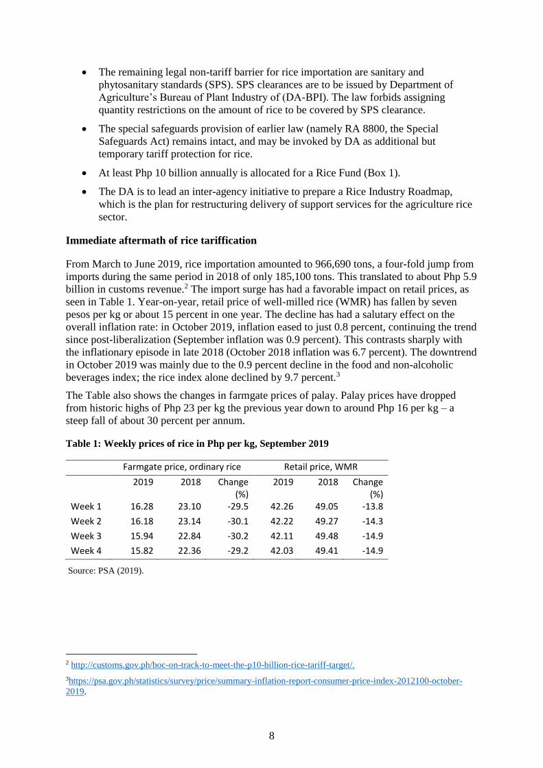
Immediate aftermath of rice tariffication

From March to June 2019, rice importation amounted to 966,690 tons, a four-fold jump from

imports during the same period in 2018 of only 185,100 tons. This translated to about Php 5.9

billion in customs revenue.2 The import surge has had a favorable impact on retail prices, as

seen in Table 1. Year-on-year, retail price of well-milled rice (WMR) has fallen by seven

pesos per kg or about 15 percent in one year. The decline has had a salutary effect on the

overall inflation rate: in October 2019, inflation eased to just 0.8 percent, continuing the trend

since post-liberalization (September inflation was 0.9 percent). This contrasts sharply with

the inflationary episode in late 2018 (October 2018 inflation was 6.7 percent). The downtrend

in October 2019 was mainly due to the 0.9 percent decline in the food and non-alcoholic

beverages index; the rice index alone declined by 9.7 percent.3

The Table also shows the changes in farmgate prices of palay. Palay prices have dropped

from historic highs of Php 23 per kg the previous year down to around Php 16 per kg – a

steep fall of about 30 percent per annum.

Table 1: Weekly prices of rice in Php per kg, September 2019

Farmgate price, ordinary rice Retail price, WMR

2019 2018 Change (%)

2019 2018 Change (%)

Week 1 16.28 23.10 -29.5 42.26 49.05 -13.8

Week 2 16.18 23.14 -30.1 42.22 49.27 -14.3

Week 3 15.94 22.84 -30.2 42.11 49.48 -14.9

Week 4 15.82 22.36 -29.2 42.03 49.41 -14.9

Source: PSA (2019).

2 http://customs.gov.ph/boc-on-track-to-meet-the-p10-billion-rice-tariff-target/.

3https://psa.gov.ph/statistics/survey/price/summary-inflation-report-consumer-price-index-2012100-october-

2019.

9

The impact of the law therefore differs sharply between rice consumers and rice producers

along the value chain. Availability of cheap imports will tend to pull down the retail price;

this redounds to the benefit of net rice consumers, i.e. those whose consumption of rice

exceeds their production (which for the vast majority of households is zero). 4 Beneficiaries

includes most of the urban consumers (about half the population), as well as rural consumers

not primarily producing rice, including producers of corn, coconut, sugarcane, and fisherfolk.

4 The League of Cities of the Philippines, has acknowledged the huge benefit of the law to their respective

constituencies, who now enjoy more affordable prices of rice. See:

https://businessmirror.com.ph/2019/09/03/for-supporting-liberalization-of-rice-imports-dof-applauded-by-

mayors/.

Box 1: The Rice Competitiveness Enhancement fund

The Rice Competitiveness Enhancement Fund or Rice Fund is equivalent to Php 10 billion per year, plus any “excess revenues”, i.e. rice tariff collections in excess of Php 10 billion. Beneficiaries of the Fund are farmers, farmworkers, and their dependents listed in the Registry System for Basic Sectors in Agriculture (RSBSA) and DA-accredited rice cooperatives and associations. Preferential attention will be accorded to rice farmers, cooperatives, and associations adversely affected by tariffication.

The Php 10 billion component of the Fund will be allocated for the next six years as follows:

1) Php 5 billion for rice farm mechanization: The Philippine Center for Postharvest Development and Mechanization (PhilMech) will provide in-kind grants of rice farm machineries and equipment to eligible farmer associations, registered rice cooperatives, and local government units (LGUs). These machineries and equipment include tilers, tractors, seeders, threshers, planters, harvesters, irrigation pumps, small solar irrigation, reapers, driers, millers, and the like.

2) Php 3 billion for rice seed development, propagation, and promotion: the Philippine Rice Research Institute (PhilRice) will develop, propagate, and promote inbred rice seeds to rice farmers; as well as organize rice farmers into seed growers associations and/or cooperatives.

3) Php 1 billion for rice credit assistance: Land Bank of the Philippines (LBP) and Development Bank of the Philippines (DBP) shall each administer a Php 0.5 billion a credit facility for rice farmers and cooperatives, imposing minimal interest charges and collateral requirements.

4) Php 1 billion for rice extension, of which Php 700 million are allocated to the Technical Education and Skills Development Authority (TESDA), and Php 100 million each to Agricultural Training Institute (ATI) of DA, Philmech, and PhilRice, for teaching skills on rice crop production, modern rice farming techniques, etc. through farm schools.

Excess revenues may be allocated to the following uses:

• Rice farmer financial assistance – for rice farmers faring two hectares and below, regardless of whether they continue rice farming;

• Individual titling of agricultural rice lands distributed under the Comprehensive Agrarian Reform Program (CARP) and similar government programs;

• Expanded crop insurance program on rice

• Crop diversification program for erstwhile rice farmers.

10

Poorer individuals who devote more of their household budget on rice will presumably

receive a greater proportional benefit.

However, the same cheap imports allow traders to quote lower palay prices, likewise pulling

down the farmgate price. Hence the reform has dealt a blow to net rice producers who

produce more rice than they consume, e.g. rice farmers, who are located nationwide, but are

concentrated most heavily in Regions II, III, VI, and XII.

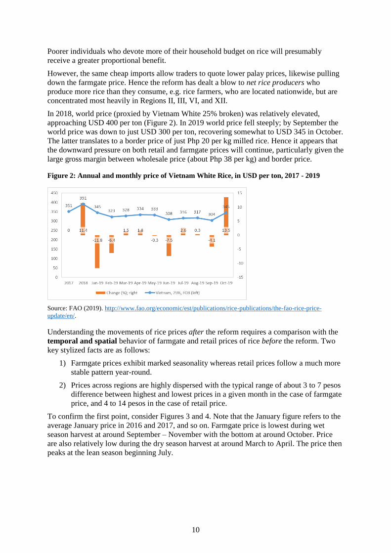
In 2018, world price (proxied by Vietnam White 25% broken) was relatively elevated,

approaching USD 400 per ton (Figure 2). In 2019 world price fell steeply; by September the

world price was down to just USD 300 per ton, recovering somewhat to USD 345 in October.

The latter translates to a border price of just Php 20 per kg milled rice. Hence it appears that

the downward pressure on both retail and farmgate prices will continue, particularly given the

large gross margin between wholesale price (about Php 38 per kg) and border price.

Figure 2: Annual and monthly price of Vietnam White Rice, in USD per ton, 2017 - 2019

Source: FAO (2019). http://www.fao.org/economic/est/publications/rice-publications/the-fao-rice-price-

update/en/.

Understanding the movements of rice prices after the reform requires a comparison with the

temporal and spatial behavior of farmgate and retail prices of rice before the reform. Two

key stylized facts are as follows:

1) Farmgate prices exhibit marked seasonality whereas retail prices follow a much more

stable pattern year-round.

2) Prices across regions are highly dispersed with the typical range of about 3 to 7 pesos

difference between highest and lowest prices in a given month in the case of farmgate

price, and 4 to 14 pesos in the case of retail price.

To confirm the first point, consider Figures 3 and 4. Note that the January figure refers to the

average January price in 2016 and 2017, and so on. Farmgate price is lowest during wet

season harvest at around September – November with the bottom at around October. Price

are also relatively low during the dry season harvest at around March to April. The price then

peaks at the lean season beginning July.

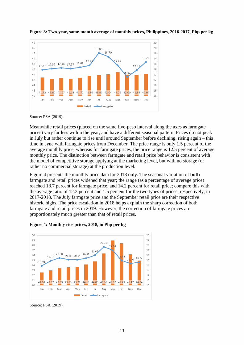
11

Figure 3: Two-year, same-month average of monthly prices, Philippines, 2016-2017, Php per kg

Source: PSA (2019).

Meanwhile retail prices (placed on the same five-peso interval along the axes as farmgate

prices) vary far less within the year, and have a different seasonal pattern. Prices do not peak

in July but rather continue to rise until around September before declining, rising again – this

time in sync with farmgate prices from December. The price range is only 1.5 percent of the

average monthly price, whereas for farmgate prices, the price range is 12.5 percent of average

monthly price. The distinction between farmgate and retail price behavior is consistent with

the model of competitive storage applying at the marketing level, but with no storage (or

rather no commercial storage) at the production level.

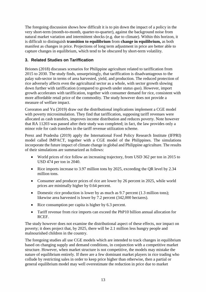
Figure 4 presents the monthly price data for 2018 only. The seasonal variation of both

farmgate and retail prices widened that year; the range (as a percentage of average price)

reached 18.7 percent for farmgate price, and 14.2 percent for retail price; compare this with

the average ratio of 12.3 percent and 1.5 percent for the two types of prices, respectively, in

2017-2018. The July farmgate price and the September retail price are their respective

historic highs. The price escalation in 2018 helps explain the sharp correction of both

farmgate and retail prices in 2019. However, the correction of farmgate prices are

proportionately much greater than that of retail prices.

Figure 4: Monthly rice prices, 2018, in Php per kg

Source: PSA (2019).

12

Regarding the second point, consider a longer time series of farmgate and retail prices

together with measures of dispersion across regions (Figures 5 and 6). The upper figure

corresponds to farmgate price. The highest levels of farmgate price prior to 2018 were in

mid-2014. In 2014-15 the coefficient of variation (quarterly average) was in the range of 8-10

percent of the mean.

Figure 5: Indicators for monthly farmgate price, June 2014 – June 2015

Source: PSA (2019).

The coefficient increased in 2015 before dropping off again in 2017; throughout 2018, when

farmgate prices soared, regional dispersion of monthly price varied by only 6-8 percent.

Starting 2019 however the variation across space started to increase breaching 11 percent by

June 2019.

The lower figure corresponds to retail price. Coefficient of variation for retail price across

regions is much smaller than that of farmgate price. The movement over time of the

coefficient tracks that of farmgate price, but not as erratically. Most important, the dispersion

of regional prices declines from final quarter of 2018 onward, the exact opposite of the

direction of change for farmgate price.

Figure 6: Monthly retail price, level and coefficient of variation (three-month average), June

2014 – June 2015

Source: PSA (2019).

13

The foregoing discussion shows how difficult it is to pin down the impact of a policy in the

very short-term (month-to-month, quarter-to-quarter), against the background noise from

natural market variation and intermittent shocks (e.g. due to climate). Within this horizon, it

is difficult to distinguish transition to equilibrium from change in equilibrium, as both

manifest as changes in price. Projections of long term adjustment in price are better able to

capture changes in equilibrium, which tend to be obscured by short-term volatility.

3. Related Studies on Tariffication

Briones (2018) discusses scenarios for Philippine agriculture related to tariffication from

2015 to 2030. The study finds, unsurprisingly, that tariffication is disadvantageous to the

palay sub-sector in terms of area harvested, yield, and production. The reduced protection of

rice adversely affects even the agricultural sector as a whole, with sector growth slowing

down further with tariffication (compared to growth under status quo). However, import

growth accelerates with tariffication, together with consumer demand for rice, consistent with

more affordable retail price of the commodity. The study however does not provide a

measure of welfare impact.

Cororaton and Yu (2019) draw out the distributional implications implement a CGE model

with poverty microsimulation. They find that tariffication, supposing tariff revenues were

allocated as cash transfers, improves income distribution and reduces poverty. Note however

that RA 11203 was passed after their study was completed; in fact, the law provides only a

minor role for cash transfers in the tariff revenue utilization scheme.

Perez and Pradesha (2019) apply the International Food Policy Research Institute (IFPRI)

model called IMPACT, together with a CGE model of the Philippines. The simulations

incorporate the future impact of climate change in global and Philippine agriculture. The results

of their simulations are summarized as follows:

• World prices of rice follow an increasing trajectory, from USD 362 per ton in 2015 to

USD 474 per ton in 2040.

• Rice imports increase to 3.97 million tons by 2025, exceeding the QR level by 2.34

million tons.

• Consumer and producer prices of rice are lower by 26 percent in 2025, while world

prices are minimally higher by 0.64 percent.

• Domestic rice production is lower by as much as 9.7 percent (1.3 million tons);

likewise area harvested is lower by 7.2 percent (342,000 hectares).

• Rice consumption per capita is higher by 6.3 percent.

• Tariff revenue from rice imports can exceed the PhP10 billion annual allocation for

RCEF.

The study however does not examine the distributional aspect of these effects, nor impact on

poverty; it does project that, by 2025, there will be 2.1 million less hungry people and

malnourished children in the country.

The foregoing studies all use CGE models which are intended to track changes in equilibrium

based on changing supply and demand conditions, in conjunction with a competitive market

structure. However, when market structure is not competitive, the models may mistake the

nature of equilibrium entirely. If there are a few dominant market players in rice trading who

collude by restricting sales in order to keep price higher than otherwise, then a partial or

general equilibrium model may well overestimate the reduction in price due to market

14

reform. The disproportionate decline in farmgate price compared to retail price has been

regarded as symptomatic of a collusion among rice importers in controlling the release of rice

stocks. In popular parlance a “rice cartel” is said to be at work.5 Furthermore, the retail price

of Php 40 per kg, corresponding to a Php 38 per kg wholesale price, is nearly double the

border price – an enormous rent that has yet to be arbitraged away.

Briones (2019) examines the rice market in detail to ascertain the degree of competition

among its players. Within the domestic market, retail rice prices are found to be integrated in

the long run at the regional level. However, adjustment to long run equililibrium is a

protracted and unpredictable process. There is no dominant player or set of players at the

extreme ends of the value chain, i.e. farmers and retailers; however, at the wholesale/miller

level, the presence of dominant players cannot be ruled out. Vertical price transmission along

the marketi ng chain of rice is found to be asymmetric, suggesting short-term deviation from

competitive behavior when palay supplies run low. There are clearly troubling signs of

departure from competitive markets, warranting further investigation.

4. Methodology

AMPLE-CGE Base model

Ex ante impact assessment of rice liberalization is limited to long term adjustment of the rice

market. The base model for the assessment is AMPLE-CGE, a standard Walrasian CGE

model. The main model equations are identical to those stated in Briones (2018). Key

features of the model are as follows:

• Consumers maximize Stone-Geary utility subject to given income and prices, this

results in consumer demand functions in the form of the linear expenditure system

(LES).

• Income is obtained from sales of labor (divided into agricultural and non-agricultural

employment); earnings from capital and land; and transfers from government and

from abroad.

• Other components of final demand are: investment, determined by available savings;

government consumption, determined exogenously; and imports, based on the

Armington approach. Intermediate demand is determined by fixed coefficients

Leontief technology.

• Household savings is a fixed ratio of household income. Tax revenue is obtained from

income taxes (fixed share of household income), the value added tax, and customs

duties (ad valorem tax on import price). Government savings is the net of tax revenue,

expenditures, and household transfers.

• Domestic supply (in terms of value added) is derived from profit maximization using

constant elasticity production functions, for labor and capital input. Supply for abroad

is based on an Armington analogue on the export side.

• In the case of crop production, area harvested derived from land allocation model

based on nested constant elasticity functions for the various crops. The model

calculates a shadow value of for land which is benefit to crop farmers from an

increase in agricultural area at the margin.

5 https://www.philstar.com/business/2019/11/06/1966263/rice-cartel.

15

• A flexible exchange rate clears the current account at exogenous level of capital

inflow. Equilibrium holds at simultaneous market clearing.

Extensions to the AMPLE-CGE

The base data of the model is organized as a social accounting matrix (SAM) compiled for

2016. To extend the AMPLE-CGE set of households H is modified from elements

corresponding to rural and urban households, to elements corresponding to the ten household

per capita income deciles. Hence, the household accounts will be disaggregated into the per

capita income deciles, using shares from the 2015 FIES.

FIES data is also used to compute food demand system elasticities for calibration into the

parameters of the LES. To review, LES is expressed in AMPLE-CGE with the following

equation

,

, , ,

G H

G H G H H G G H

GG

QC qcmn XPD PD qcmnPD

= + −

(1)

The variables and parameters of (1) are defined as follows:

H Household

G Food types

,G HQC Per capita consumption

GPD Retail price

HXPD Per capita expenditure

,G Hqcmn Minimum household consumption per capita of G (subsistence)

,G H Coefficient term in LES

Let ,G Hsh denote expenditure shares. Note that (1) collapses to the Cobb-Douglas fixed

expenditure shares system in the special case that , 0G Hqcmn = with ,G H as the fixed shares.

This reflects a homothetic demand structure which is a special case of LES. When

, 0G Hqcmn then we have (1) as a general case. The more general formulation is desirable

when preference is known to be nonhomothetic, i.e. in the case of food, Engel’s Law has

been found as an empirical regularity (food staples that loom large in the food basket of the

lower income group must decline as expenditure level increases.) Equation (1), which can be

rearranged as follows:

, , , , , ,G H G H G H G H G H H G G H

G

PD QC PD qcmn XPD PD qcmn

= + −

(1’)

Refer to the bracketed term in (1’) as supernumerary expenditure, i.e. the expenditure level in

excess of the value of minimum purchases of the household. Then expenditure is a linear

function of supernumerary expenditure rather than actual expenditure, as in the case of

homothetic preference. However, as expenditures keep rising then supernumerary and total

expenditure converge, and demand behavior converges to the case of homothetic preference.

Expenditure and own-price elasticities, respectively denoted ,G H and ,G H are computed

based on the following formulas (Annabi et al, 2006):

16

,

,

,

G H

G H

G Hsh

= ; (2)

( ), ,

,

,

11

G H G H

G H

G H

qcmn

QD

− = − . (3)

Parameter to be estimated are ,G H and ,G Hqcmn . To estimate these, we first organize FIES

as follows:

• Identify the FIES food types that approximately match the AMPLE-CGE food types.

Expenditure items are then aggregated for the purpose of estimation. The food types

for estimation are: Corn, Coconut, Banana, Mango, Other fruit, Rootcrop, Vegetables,

Poultry, Capture Fisheries, Aquaculture, Rice, Processed Fish, Sugar, Meat products.

• Retail prices of the matching FIES food types are then assembled by region; each

household is assumed to face the same set of retail prices.

• Total and item-specific expenditure of the foregoing food types is assembled from the

FIES to estimate Equation (1). Estimation adopts the nonlinear seemingly unrelated

regression method; in Stata this is implemented by the command nlsur.

• Using the parameter estimates, elasticities given in (2) and (3) are then evaluated at

the sample means disaggregated by per capita income decile. (Parameters that result

in counter-intuitive elasticities are replaced by imputed value). The elasticities based

on estimation are then used to inform the LES elasticities used in the AMPLE-CGE.

Prices and expenditure shares are shown in Table 2. Note that the shares are computed in

terms of the limited food types on the first column. Hence, rice expenditure share starts out at

41 percent for the lowest decile; the share declines as the income decile rises, as expected

from Engel’s law. However, the decline is gradual; at the top income decile the rice

expenditure share is still 38 percent. For the other food types, the shares remain similar across

deciles, or decline gradually as income group increases, with the exception of meat products

where the expenditure shares clearly rise with income.

Table 2: Prices (Php per unit) and expenditure shares by decile, Philippines, 2015

Prices Expenditure shares (%)

1 2 3 4 5 6 7 8 9 10

Corn 25.04 3.9 2.6 3.6 3.5 3.4 3.3 3.1 3.0 2.9 2.7

Coconut 20.87 0.6 0.5 0.6 0.6 0.6 0.6 0.6 0.6 0.6 0.6

Banana 49.79 1.9 2.1 2.0 2.0 2.0 2.0 2.0 2.0 2.0 2.0

Mango 80.94 0.9 0.9 0.9 0.9 0.9 0.9 0.9 0.9 0.9 0.9

Other fruit 36.68 0.3 0.3 0.3 0.3 0.3 0.3 0.3 0.3 0.3 0.3

Rootcrop 32.26 0.7 0.5 0.7 0.7 0.6 0.6 0.6 0.6 0.6 0.5

Vegetables 59.58 10.5 9.9 10.4 10.3 10.3 10.2 10.1 10.0 10.0 9.9

Poultry 137.50 6.3 7.5 6.6 6.6 6.8 6.9 7.0 7.1 7.2 7.3

Capture Fisheries 178.04 5.6 6.0 5.7 5.7 5.8 5.8 5.9 5.9 6.0 6.0

Aquaculture 117.58 5.5 6.4 5.7 5.8 5.9 6.0 6.1 6.1 6.2 6.3

Rice 42.04 40.5 37.9 39.9 39.8 39.5 39.2 38.9 38.7 38.5 38.2

Processed Fish 86.96 4.2 3.6 4.1 4.1 4.0 3.9 3.8 3.8 3.7 3.7

Sugar 45.96 2.3 1.8 2.2 2.1 2.1 2.0 2.0 2.0 1.9 1.9

Meat products 235.78 16.6 20.0 17.4 17.5 17.9 18.3 18.8 19.0 19.3 19.6

Source: PSA (2018).

17

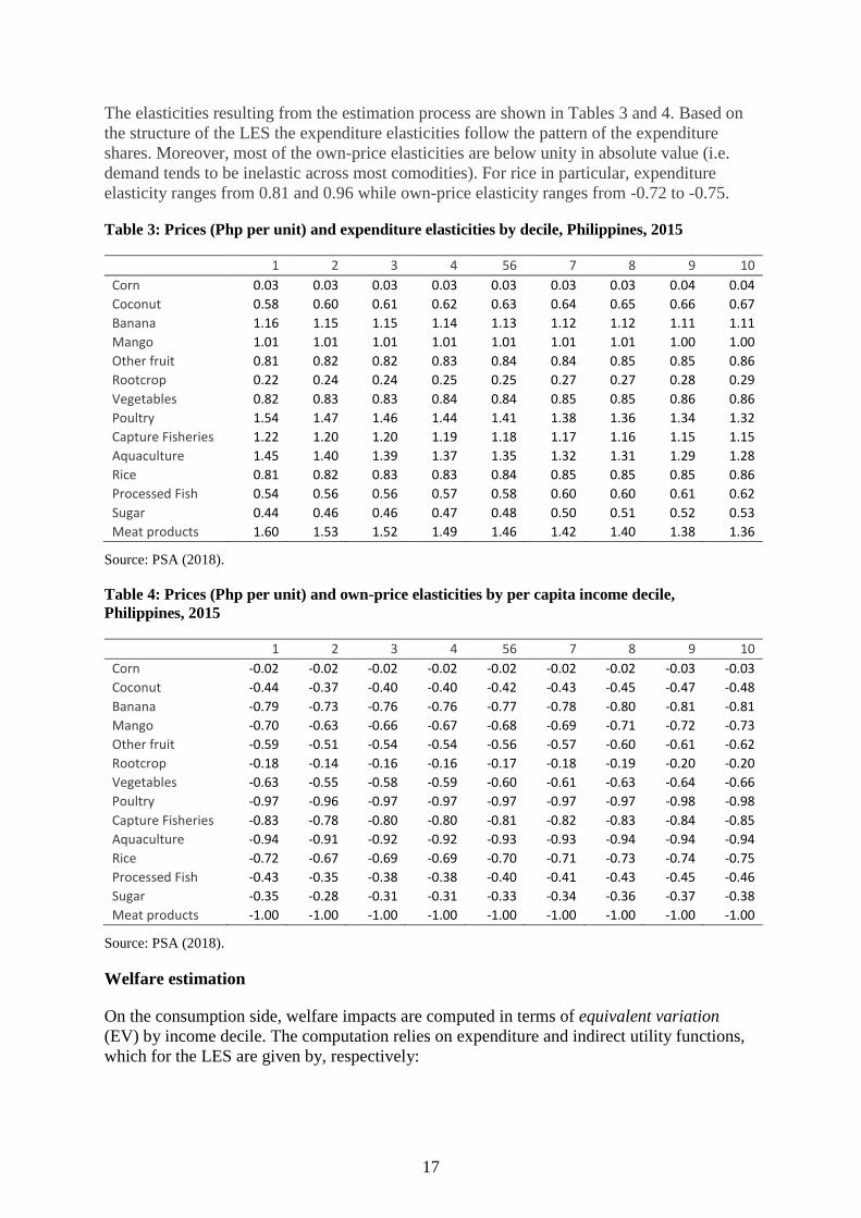
The elasticities resulting from the estimation process are shown in Tables 3 and 4. Based on

the structure of the LES the expenditure elasticities follow the pattern of the expenditure

shares. Moreover, most of the own-price elasticities are below unity in absolute value (i.e.

demand tends to be inelastic across most comodities). For rice in particular, expenditure

elasticity ranges from 0.81 and 0.96 while own-price elasticity ranges from -0.72 to -0.75.

Table 3: Prices (Php per unit) and expenditure elasticities by decile, Philippines, 2015

1 2 3 4 56 7 8 9 10

Corn 0.03 0.03 0.03 0.03 0.03 0.03 0.03 0.04 0.04

Coconut 0.58 0.60 0.61 0.62 0.63 0.64 0.65 0.66 0.67

Banana 1.16 1.15 1.15 1.14 1.13 1.12 1.12 1.11 1.11

Mango 1.01 1.01 1.01 1.01 1.01 1.01 1.01 1.00 1.00

Other fruit 0.81 0.82 0.82 0.83 0.84 0.84 0.85 0.85 0.86

Rootcrop 0.22 0.24 0.24 0.25 0.25 0.27 0.27 0.28 0.29

Vegetables 0.82 0.83 0.83 0.84 0.84 0.85 0.85 0.86 0.86

Poultry 1.54 1.47 1.46 1.44 1.41 1.38 1.36 1.34 1.32

Capture Fisheries 1.22 1.20 1.20 1.19 1.18 1.17 1.16 1.15 1.15

Aquaculture 1.45 1.40 1.39 1.37 1.35 1.32 1.31 1.29 1.28

Rice 0.81 0.82 0.83 0.83 0.84 0.85 0.85 0.85 0.86

Processed Fish 0.54 0.56 0.56 0.57 0.58 0.60 0.60 0.61 0.62

Sugar 0.44 0.46 0.46 0.47 0.48 0.50 0.51 0.52 0.53

Meat products 1.60 1.53 1.52 1.49 1.46 1.42 1.40 1.38 1.36

Source: PSA (2018).

Table 4: Prices (Php per unit) and own-price elasticities by per capita income decile,

Philippines, 2015

1 2 3 4 56 7 8 9 10

Corn -0.02 -0.02 -0.02 -0.02 -0.02 -0.02 -0.02 -0.03 -0.03

Coconut -0.44 -0.37 -0.40 -0.40 -0.42 -0.43 -0.45 -0.47 -0.48

Banana -0.79 -0.73 -0.76 -0.76 -0.77 -0.78 -0.80 -0.81 -0.81

Mango -0.70 -0.63 -0.66 -0.67 -0.68 -0.69 -0.71 -0.72 -0.73

Other fruit -0.59 -0.51 -0.54 -0.54 -0.56 -0.57 -0.60 -0.61 -0.62

Rootcrop -0.18 -0.14 -0.16 -0.16 -0.17 -0.18 -0.19 -0.20 -0.20

Vegetables -0.63 -0.55 -0.58 -0.59 -0.60 -0.61 -0.63 -0.64 -0.66

Poultry -0.97 -0.96 -0.97 -0.97 -0.97 -0.97 -0.97 -0.98 -0.98

Capture Fisheries -0.83 -0.78 -0.80 -0.80 -0.81 -0.82 -0.83 -0.84 -0.85

Aquaculture -0.94 -0.91 -0.92 -0.92 -0.93 -0.93 -0.94 -0.94 -0.94

Rice -0.72 -0.67 -0.69 -0.69 -0.70 -0.71 -0.73 -0.74 -0.75

Processed Fish -0.43 -0.35 -0.38 -0.38 -0.40 -0.41 -0.43 -0.45 -0.46

Sugar -0.35 -0.28 -0.31 -0.31 -0.33 -0.34 -0.36 -0.37 -0.38

Meat products -1.00 -1.00 -1.00 -1.00 -1.00 -1.00 -1.00 -1.00 -1.00

Source: PSA (2018).

Welfare estimation

On the consumption side, welfare impacts are computed in terms of equivalent variation

(EV) by income decile. The computation relies on expenditure and indirect utility functions,

which for the LES are given by, respectively:

18

( ),

,

, , ,

,

,

G H

G H

G H G H G H

G G G H

PDE PD u PD qcmn u

= +

; (4)

,

,

,

,

( , )

G H

G H

G H H

G G H

V PD XPDPD

=

. (5)

Here u denotes a given utility level. Given two sets of prices, 0

,G HPD , 1

,G HPD , with

corresponding (maximum) utility levels 0u , and 1u , the general formula for EV is:

( )0 1 0 0

, ,, ( , )G H G HEV E PD u E PD u= − . (6)

Utility is evaluated using (5), while E is evaluated using (4). Of course, total welfare of the

households is obtained by multiplying EV with the respective population.

In addition to consumer welfare through changes in price, welfare also adjusts on the

producer side through changes in income. Strictly speaking the AMPLE-CGE adopts constant

returns technology hence equilibrium implies zero profits. In the model, value added is paid

out as rental income to capital, wage income to labor, and the residual as returns to deploying

land. The last therefore is our measure of palay farmers’ welfare PW.

Note that the residual character of returns to land is still valid even if a component of it were

allocated as fixed rental for landowners. The sole exception would be share tenancy, which is

illegal under Philippine law; in 2002, only 7.2. percent of palay farm area was sharecropped

(Ballesteros, 2006). Since then, government land reform has progressed to break up large

estates and suppress share tenancy.

Let NREV denote net income per ha and HC the total area harvested for palay; subscripts 1

and 0 denote alternative and reference scenarios, respectively. A simple calculation of change

in palay farmers’ income as a group is therefore the following:

1 0 1 1 0 0.PW PW PW NREV HC NREV HC = − = − (7)

However, the aforementioned formula does not fix the cropped area of palay farmers at the

baseline, though presumably the same farmers are able to realize some returns from

deploying their land to another crop. To account for this the income of palay farmers under

the alternative scenario is computed as follows:

( )1 1 1 0 1PW NREV HC HC HC= + − . (8)

Here denotes the shadow price of land. The first term denotes the return from the current

cropped area for palay; the second term is the shift out of palay into other crops, whose return

is valued at the shadow price. We therefore calculate 1PW using (8). Both producer income

change and consumer welfare change over time expressed in net present value using a social

discount rate (assumed equal to 5 percent).

Set-up of scenarios

The reference scenario (without) corresponds to the status quo without tariffication. The

AMPLE-CGE contains an expression for non-tariff barrier ntb, expressed as an ad valorem

implicit tariff which for rice is calibrated at the base data set at ntb = 0.74. Scenarios are

solved from 2016 (the base year of the SAM) every year to 2030.

19

The reference scenario adopts exogenous variable projections for population growth,

technological change, and world price, as reported by Briones (2018) but with ntb held at the

base value. The alternative scenario (with) meanwhile has identical exogenous variables but

with ntb shrunk to 99 percent of its base value in one year (representing residual non-tariff

barriers in the rice sub-sector).

5. Results

The following shows simulation results for the rice sub-sector divided into five-year intervals

(2019-2024 and 2025-2030); simulations for 2016-2018 are omitted as these are identical

between reference and alternative scenarios.

Imports

Growth of rice imports with and without liberalization is shown in Figure 7. In the reference

case, imports are projected to grow initially by only 7 percent per year, accelerating mildly to

7.23 percent by 2025-30. In contrast, average annual growth of imports in 2019-24 is 53

percent per year, decelerating to 5 percent in 2025-30, for an average growth of 29.1 percent

over the period. The net change is 22 percentage points for import growth owing to

liberalization.

Figure 7: Rice import growth projections by scenario, 2019 – 2030 (%)

Source: Author’s calculation.

Palay production and area harvested

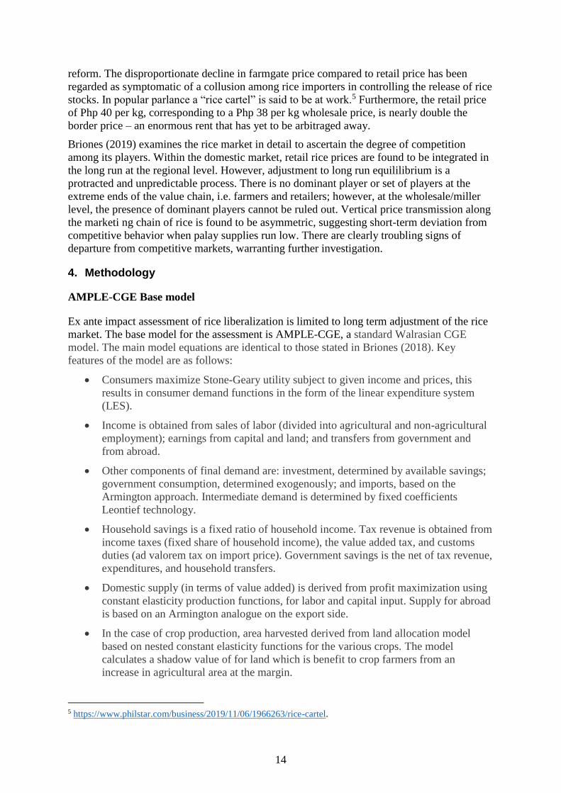
Production of palay is projected to grow initially at 2.8 percent per year in the absence of

tariffication, decelerating gently to 2.3 percent. With tariffication, palay production contracts

initially averaging -5.7 percent decline up to 2024, but posting positive growth on average

from 2025 onward. The net difference is an 8.5 percentage point reduction up to 2024 and a

0.2 percentage point reduction up to 2030.

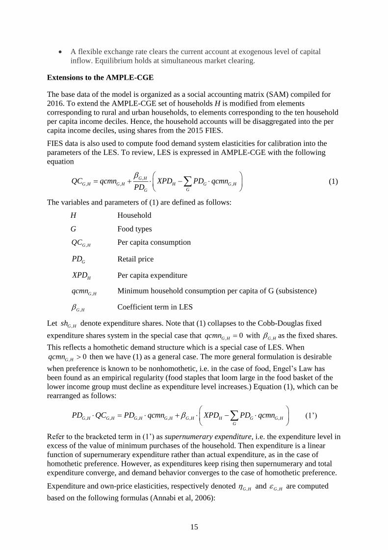
Without liberalization, area harvested for palay is projected to grow, by 1 percent per year to

2024, then 0.7 percent p.a. to 2030 (Figure 9). With liberalization, area harvested will

contract by 3.3 percent p.a., reversing to an expansion by 0.4 percent per year to 2030. The

difference is a total of -4.4 percent point change to 2024, or -2.0 percentage points for the

whole projection period.

20

Figure 8: Rice production growth projections, by scenario, 2019 – 2030 (%)

Source: Author’s calculation.

Figure 9: Rice area harvested growth projections, by scenario, 2019 – 2030 (%)

Source: Author’s calculation.

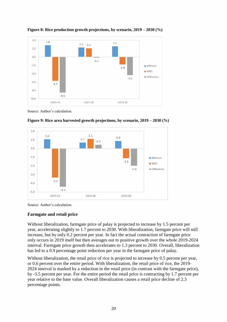
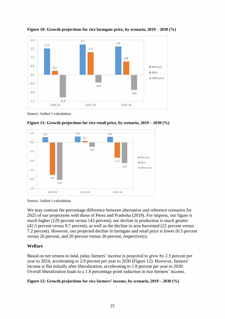
Farmgate and retail price

Without liberalization, farmgate price of palay is projected to increase by 1.5 percent per

year, accelerating slightly to 1.7 percent to 2030. With liberalization, farmgate price will still

increase, but by only 0.2 percent per year. In fact the actual contraction of farmgate price

only occurs in 2019 itself but then averages out to positive growth over the whole 2019-2024

interval. Farmgate price growth then accelerates to 1.3 percent to 2030. Overall, liberalization

has led to a 0.9 percentage point reduction per year in the farmgate price of palay.

Without liberalization, the retail price of rice is projected to increase by 0.5 percent per year,

or 0.6 percent over the entire period. With liberalization, the retail price of rice, the 2019-

2024 interval is marked by a reduction in the retail price (in contrast with the farmgate price),

by -3.5 percent per year. For the entire period the retail price is contracting by 1.7 percent per

year relative to the base value. Overall liberalization causes a retail price decline of 2.3

percentage points.

21

Figure 10: Growth projections for rice farmgate price, by scenario, 2019 – 2030 (%)

Source: Author’s calculation.

Figure 11: Growth projections for rice retail price, by scenario, 2019 – 2030 (%)

Source: Author’s calculation.

We may contrast the percentage difference between alternative and reference scenarios for

2025 of our projections with those of Perez and Pradesha (2019). For imports, our figure is

much higher (229 percent versus 143 percent); our decline in production is much greater

(42.5 percent versus 9.7 percent), as well as the decline in area harvested (22 percent versus

7.2 percent). However, our projected decline in farmgate and retail price is lower (6.5 percent

versus 26 percent, and 20 percent versus 26 percent, respectively).

Welfare

Based on net returns to land, palay farmers’ income is projected to grow by 2.5 percent per

year to 2024, accelerating to 2.9 percent per year to 2030 (Figure 12). However, farmers’

income is flat initially after liberalization, accelerating to 1.8 percent per year to 2030.

Overall liberalization leads to a 1.8 percentage point reduction in rice farmers’ income.

Figure 12: Growth projections for rice farmers’ income, by scenario, 2019 – 2030 (%)

22

Source: Author’s calculation.

The first column of Table 5 shows the allocation of the net income from land across the

deciles using income shares, assumed to be fixed throughout the projection period. The

shares were calculated as follows:

• The 2015 FIES were merged with the 2015 Labor Force Survey (October round).

Palay farming households are distinguished in the sample by i) identifying households

whose heads have palay farming as their primary occupation; and ii) among these

households, identifying those whose net crop income exceeds their expenditure on

rice (i.e. the net rice producers).

• For palay farming households, the entire net crop income from farming are used to

compute shares by decile (using per capita income decile indicator in the merged data

set); this assumes that palay farming income is distributed the same way net crop

income, at least for palay farming households.

Table 5: Impact on rice farmers’ income by decile, 2019 – 2030 (Php millions, fixed 2016 prices)

Shares in palay farmers household income (%)

2019-24 2025-30 2019-30

H1 13.5 -905 -1,507 -1,206

H2 14.2 -1,038 -1,728 -1,383

H3 12.3 -945 -1,573 -1,259

H4 13.1 -985 -1,639 -1,312

H5 10.0 -751 -1,251 -1,001

H6 8.7 -688 -1,146 -917

H7 9.2 -694 -1,156 -925

H8 7.3 -583 -971 -777

H9 6.8 -568 -946 -757

H10 5.0 -403 -672 -537

Total 100.0 -7,560 -12,589 -10,075

Source: Author’s calculation.

Note that the largest shares in palay farmers’ income are clearly in the lowest deciles.

However, the share remains significant even as the income deciles go up; the top decile

accounts for 5.3 percent of palay farmers’ income. Note that poverty incidence in 2015 was

23

21.6 percent, hence poverty mostly overlaps with the first two deciles; these two deciles

account for just 25.7 percent of palay farmers’ income.

Based on these shares, the change in palay farmers’ income is allocated to the deciles as

shown in the next three columns of Table 5. The largest impact of course is on the second

decile (given it has the largest share), followed by the first fourth, third, and first (poorest)

deciles. The negative impact in producers’ welfare worsens over time. Loss in rice farmers’

income is up to Php 7.6 billion per year in 2016 prices to 2024, rising to Php 12.6 billion per

year to 2030, for an average reduction of about Php 10 billion per year. The amount is

auspiciously close to the minimum allocation for the Rice Fund.

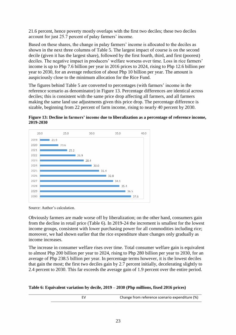
The figures behind Table 5 are converted to percentages (with farmers’ income in the

reference scenario as denominator) in Figure 13. Percentage differences are identical across

deciles; this is consistent with the same price drop affecting all farmers, and all farmers

making the same land use adjustments given this price drop. The percentage difference is

sizable, beginning from 22 percent of farm income, rising to nearly 40 percent by 2030.

Figure 13: Decline in farmers’ income due to liberalization as a percentage of reference income,

2019-2030

Source: Author’s calculation.

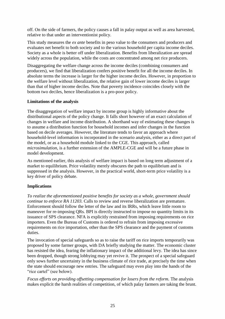
Obviously farmers are made worse off by liberalization; on the other hand, consumers gain

from the decline in retail price (Table 6). In 2019-24 the increment is smallest for the lowest

income groups, consistent with lower purchasing power for all commodities including rice;

moreover, we had shown earlier that the rice expenditure share changes only gradually as

income increases.

The increase in consumer welfare rises over time. Total consumer welfare gain is equivalent

to almost Php 200 billion per year to 2024, rising to Php 280 billion per year to 2030, for an

average of Php 238.5 billion per year. In percentage terms however, it is the lowest deciles

that gain the most; the first two deciles gain by 2.7 percent initially, decelerating slightly to

2.4 percent to 2030. This far exceeds the average gain of 1.9 percent over the entire period.

Table 6: Equivalent variation by decile, 2019 – 2030 (Php millions, fixed 2016 prices)

EV Change from reference scenario expenditure (%)

24

2019-24 2025-30 2019-30 2019-24 2025-30 2019-30

H1 9,403 10,361 9,882 2.7 2.3 2.5

H2 12,604 15,292 13,948 2.7 2.5 2.6

H3 14,462 18,850 16,656 2.7 2.6 2.7

H4 16,605 22,557 19,581 2.6 2.6 2.6

H5 18,927 26,604 22,765 2.5 2.6 2.5

H6 20,615 29,531 25,073 2.2 2.4 2.3

H7 22,599 33,051 27,825 2.1 2.3 2.2

H8 24,390 36,120 30,255 1.9 2.0 1.9

H9 26,204 39,148 32,676 1.5 1.7 1.6

H10 31,657 48,037 39,847 1.1 1.2 1.1

Total 197,467 279,550 238,509 1.8 1.9 1.9

Source: Author’s calculation.

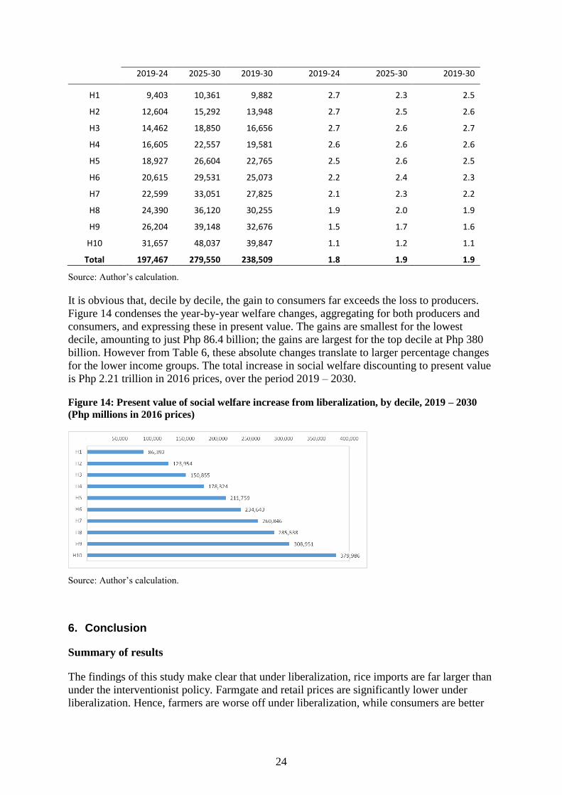
It is obvious that, decile by decile, the gain to consumers far exceeds the loss to producers.

Figure 14 condenses the year-by-year welfare changes, aggregating for both producers and

consumers, and expressing these in present value. The gains are smallest for the lowest

decile, amounting to just Php 86.4 billion; the gains are largest for the top decile at Php 380

billion. However from Table 6, these absolute changes translate to larger percentage changes

for the lower income groups. The total increase in social welfare discounting to present value

is Php 2.21 trillion in 2016 prices, over the period 2019 – 2030.

Figure 14: Present value of social welfare increase from liberalization, by decile, 2019 – 2030

(Php millions in 2016 prices)

Source: Author’s calculation.

6. Conclusion

Summary of results

The findings of this study make clear that under liberalization, rice imports are far larger than

under the interventionist policy. Farmgate and retail prices are significantly lower under

liberalization. Hence, farmers are worse off under liberalization, while consumers are better

25

off. On the side of farmers, the policy causes a fall in palay output as well as area harvested,

relative to that under an interventionist policy.

This study measures the ex ante benefits in peso value to the consumers and producers and

evaluates net benefit to both society and to the various household per capita income deciles.

Society as a whole is better off under liberalization. Benefits from liberalization are spread

widely across the population, while the costs are concentrated among net rice producers.

Disaggregating the welfare change across the income deciles (combining consumers and

producers), we find that liberalization confers positive benefit for all the income deciles. In

absolute terms the increase is larger for the higher income deciles. However, in proportion to

the welfare level without liberalization, the relative gain of lower income deciles is larger

than that of higher income deciles. Note that poverty incidence coincides closely with the

bottom two deciles, hence liberalization is a pro-poor policy.

Limitations of the analysis

The disaggregation of welfare impact by income group is highly informative about the

distributional aspects of the policy change. It falls short however of an exact calculation of

changes in welfare and income distribution. A shorthand way of estimating these changes is

to assume a distribution function for household incomes and infer changes in the function

based on decile averages. However, the literature tends to favor an approach where

household-level information is incorporated in the scenario analysis, either as a direct part of

the model, or as a household module linked to the CGE. This approach, called

microsimulation, is a further extension of the AMPLE-CGE and will be a future phase in

model development.

As mentioned earlier, this analysis of welfare impact is based on long term adjustment of a

market to equilibrium. Price volatility merely obscures the path to equilibrium and is

suppressed in the analysis. However, in the practical world, short-term price volatility is a

key driver of policy debate.

Implications

To realize the aforementioned positive benefits for society as a whole, government should

continue to enforce RA 11203. Calls to review and reverse liberalization are premature.

Enforcement should follow the letter of the law and its IRRs, which leave little room to

maneuver for re-imposing QRs. BPI is directly instructed to impose no quantity limits in its

issuance of SPS clearance. NFA is explicitly restrained from imposing requirements on rice

importers. Even the Bureau of Customs is ordered to refrain from imposing excessive

requirements on rice importation, other than the SPS clearance and the payment of customs

duties.

The invocation of special safeguards so as to raise the tariff on rice imports temporarily was

proposed by some farmer groups, with DA briefly studying the matter. The economic cluster

has resisted the idea, fearing the inflationary impact of the additional levy. The idea has since

been dropped, though strong lobbying may yet revive it. The prospect of a special safeguard

only sows further uncertainty in the business climate of rice trade, at precisely the time when

the state should encourage new entries. The safeguard may even play into the hands of the

“rice cartel” (see below).

Focus efforts on providing offsetting compensation for losers from the reform. The analysis

makes explicit the harsh realities of competition, of which palay farmers are taking the brunt.

26

The safety net provision of RA 11203 precisely anticipated this prospect and provides for

assistance to rice farmers. However, utilization of RCEF has lagged in comparison with

market movements. Agencies with hitherto no implementation function (PhilMech, PhilRice,

etc.) were suddenly mandated to administer large-scale production support programs. The

provisions of the law explicitly require procurement of various goods and services

(machineries, seeds, etc.), a process that is perennially prone to delay within the bureaucracy

(Navarro and Tanghal, 2017).

To forestall further adverse impacts on rice farmers, it seems fitting to accelerate safety net

programs for this sub-sector, such provision of targeted cash transfers (conditional only on

being a small rice farmer in areas suffering from the biggest drops in palay price). Moreover,

beyond production support, DA and related agencies should innovate by investing heavily in

participatory value chain programs to encourage rice farmer cooperatives and associations to

engage in wholesale or retail trade of rice, to be milled through facilitated toll processing.

Investigate the state of competition in rice marketing and diligently enforce competition

policy in the rice industry. Consumers have thus far reaped early gains from liberalization;

indeed, inflation has fallen to near zero in recent months, in part owing to continued decline

in the consumer price of rice.

Moreover, the drop in farmgate prices have appeared to be all out of proportion to the decline

in retail prices. This is cited by critics of liberalization as a symptom of “failure” of the law.

Note however that the liberalization came as a massive, one-time shock to the rice market

which had already experienced considerable volatility going in to the reform. In the aftermath

of the shock, we observed a sharp correction to the past escalation of farmgate prices; an

increase in dispersion of farmgate prices across regions as markets adjust differentially to the

shock. These considerations suggest that price will eventually normalize after the initial

shock plays out.

On the other hand, a large margin persists between border price and wholesale price, which in

turn props up the retail price. Moreover, there was a decrease in the regional dispersion of

retail prices. It is not a farfetched notion to see possible coordination among early adopters of

open access to foreign rice. Competition from later entrants should in principle neutralize this

coordination, but it seems to be long in coming. Uncertainty in the business climate owing to

potential policy reversal (such as special safeguards) does nothing to help encourage new

entrants and thereby healthier competition in rice trading.

To maximize benefits to rice consumers, competition policy should be invoked to investigate

thoroughly the nature of pricing in the rice market. If pricing at the wholesale and retail level

are subject to significant adjustment delays and persistently high rents, then government

intervention may be warranted in terms of enforcing competitive outcomes. This may include

penalties on hoarding and massive releases from the buffer stock. The aforementioned

program on participatory value chains will also support widening competition in rice

marketing.

Bibliography

Annabi, N., J. Cockburn, B. Decaluwe. 2006. Functional forms and parametrization of CGE

models. MPIA Working Paper 2006-04. Poverty and Economic Policy Network.

Ballesteros, M. 2008. Land Rental Market Activity in Agrarian Reform Areas: Evidence from

the Philippines. Discussion Paper Series No. 2008-26. Quezon City: PIDS.

27

Briones, R. 2018. Scenarios for the Philippine Agri-Food System with and without

Tariffication: Application of a CGE model with Endogenous Area Allocation. Discussion

Paper Series No. 2018-51. Quezon City: PIDS.

Briones, R. 2019. Competition in the rice industry: an issues paper. PCC Issues Paper No. 1,

Series of 2019. Quezon City: Philippine Competition Commission.

Cororaton, C., and K. Yu. 2019. Assessing the Poverty and Distributional Impact of

Alternative Rice Policies in the Philippines. DLSU Business & Economics Review 28(2):

169–182.

Navarro, A., and J. Tanghal. 2017. The promises and pains in procurement reforms in the

Philippines. Discussion Paper Series No. 2017-16. Quezon City: PIDS.

Perez, N., and A. Pradesha. 2019. Philippine Rice Trade Liberalization: Impacts on Agriculture

and the Economy, and Alternative Policy Actions. NEDA-IFPRI Policy Studies. 1 June 2019.