Embed Size (px)
Citation preview

Welcome to the PresentationWelcome to the Presentation
Statistical Linkage Analysis and QTL mapping
By
Dr. Md Nurul Haque MollahProfessor, Department of Statistics,University of Rajshahi, Bangladesh
1
Outline
(1) Basic Genetics
(2) Linkage Analysis and Map Construction
(3) A General Model for Linkage Analysis in Controlled
crosses
(4) QTL Analysis 1
(5) QTL Analysis 2
2Dr. M. N. H. Mollah24/03/12
Gene and Chromosome Genes are discrete units in which biological characteristics
are inherited from parents to offspring.
Genes are normally transmitted unchanged from generation to generation, and they usually occur in pairs.
If a given pair consists of similar genes, the individual is said to be homozygous for the gene in question, while if the genes are dissimilar, the individual is said to be heterozygous.
For example, if we have two alternative genes, say A and a, there are two kinds of homozygotes, namely AA and aa, and one kind of heterozygote, namely Aa.
1. Basic Genetics1. Basic Genetics
3Dr. M. N. H. Mollah24/03/12
Alternative genes are called alleles.
With a single pair of alleles, there are three different kinds of possible organisms represented by the three genotypes AA, Aa, and aa.
Genes are generally very numerous, and situated within the cell nucleus, where they lie in linear order along microscopic bodies called chromosomes.
The chromosomes occur in similar, or homologous, pairs, where the number of pairs is constant for each species.
For example, Drosophila has 4 pairs of chromosomes, pine has 12, the house mouse has 20, humans have 23, etc.
4Dr. M. N. H. Mollah24/03/12
The totality of these pairs constitutes the genome of a particular organism.
Genes are present in pairs in all cells of an adult organism, except for gametes. That is the gametes have only one gene from any given pair.
Thus if an adult has genotype AA, all the gametes produced are of type A. But if the genotype is Aa, two types of gametes are possible, A and a, and these are normally produced in equal numbers.
One of the chromosome pairs in the genome are the sex chromosomes (typically denoted by X and Y) that determine genetic sex.
5Dr. M. N. H. Mollah24/03/12
The other pairs are autosomes which guide the expression of most other traits.Each gene pair has a certain place or locus on a particular chromosome. Since the chromosomes occur in pairs, the loci and the genes occupying them also occur in pairs.
The most important purpose of a genome mapping project is to locate the genes affecting trait expressions on chromosomes.
Chromosomes are long pieces of DNA found in the center (nucleus) of cells.
6Dr. M. N. H. Mollah24/03/12
DNA is the material that holds genes It is considered the building block of the human body.
In the nucleus of each cell, the DNA molecule is packaged into thread-like structures called chromosomes. Each chromosome is made up of DNA tightly coiled many times around proteins called histones that support its structure.
Genes are the individual instructions that tell our bodies how to develop and function; they govern our physical and medical characteristics, such as hair color, blood type and susceptibility to disease.
7Dr. M. N. H. Mollah24/03/12
Loci In the fields of genetics and genetic computation,
a locus (plural loci) is the specific location of a gene or DNA sequence on a chromosome.
A variant of the DNA sequence at a given locus is called an allele.
The ordered list of loci known for a particular genome is called a genetic map.
Gene mapping is the procession of determining the locus for a particular biological trait.
Diploid and polyploid cells whose chromosomes have the same allele of a given gene at some locus are called homozygous with respect to that gene, while those that have different alleles of a given gene at a locus, are called heterozygous with respect to that gene.
8Dr. M. N. H. Mollah24/03/12
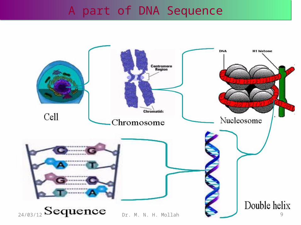
A part of DNA SequenceA part of DNA Sequence
9Dr. M. N. H. Mollah24/03/12
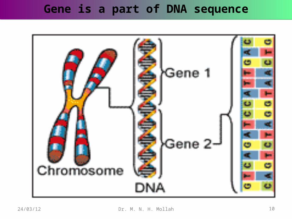
Gene is a part of DNA sequenceGene is a part of DNA sequence
10Dr. M. N. H. Mollah24/03/12
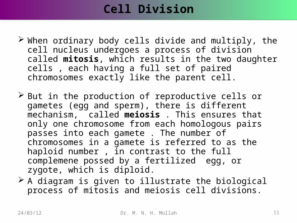
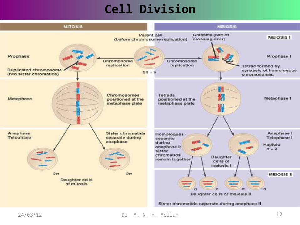
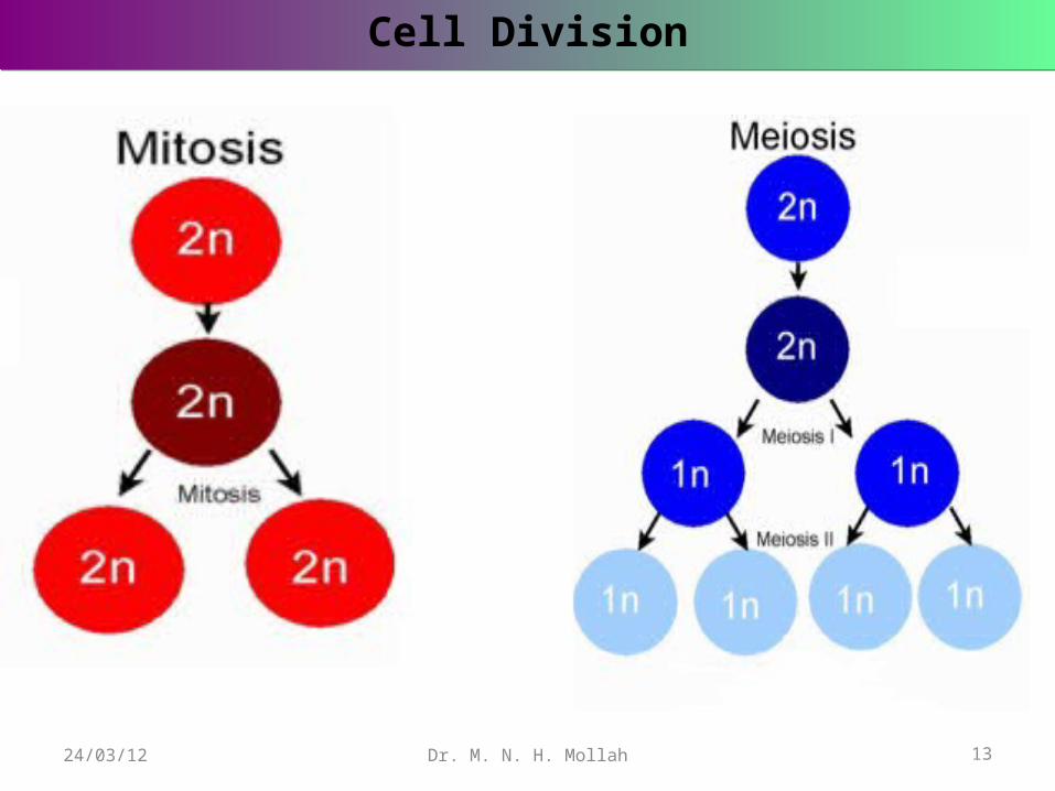
When ordinary body cells divide and multiply, the cell nucleus undergoes a process of division called mitosis, which results in the two daughter cells , each having a full set of paired chromosomes exactly like the parent cell.
But in the production of reproductive cells or gametes (egg and sperm), there is different mechanism, called meiosis . This ensures that only one chromosome from each homologous pairs passes into each gamete . The number of chromosomes in a gamete is referred to as the haploid number , in contrast to the full complemene possed by a fertilized egg, or zygote, which is diploid.
A diagram is given to illustrate the biological process of mitosis and meiosis cell divisions.
Dr. M. N. H. Mollah 11
Cell DivisionCell Division
24/03/12
Dr. M. N. H. Mollah 12
Cell DivisionCell Division
24/03/12
Dr. M. N. H. Mollah 13
Cell DivisionCell Division
24/03/12
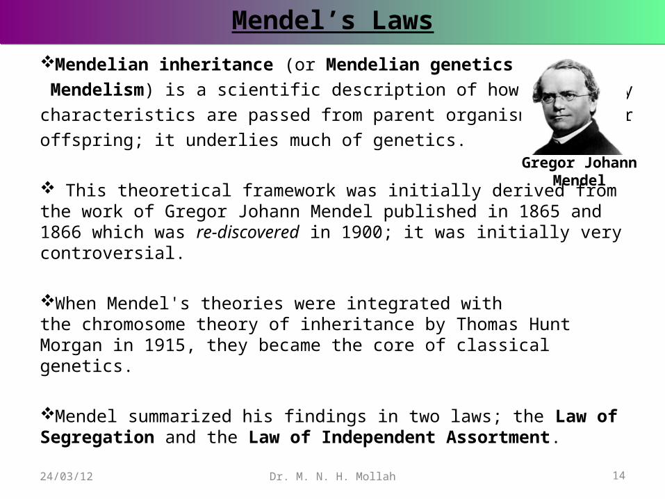
Mendelian inheritance (or Mendelian genetics or
Mendelism) is a scientific description of how hereditary
characteristics are passed from parent organisms to their
offspring; it underlies much of genetics.
This theoretical framework was initially derived from the work of Gregor Johann Mendel published in 1865 and 1866 which was re-discovered in 1900; it was initially very controversial.
When Mendel's theories were integrated with the chromosome theory of inheritance by Thomas Hunt Morgan in 1915, they became the core of classical genetics.
Mendel summarized his findings in two laws; the Law of Segregation and the Law of Independent Assortment.
Gregor Johann Mendel
Mendel’s LawsMendel’s Laws
14Dr. M. N. H. Mollah24/03/12
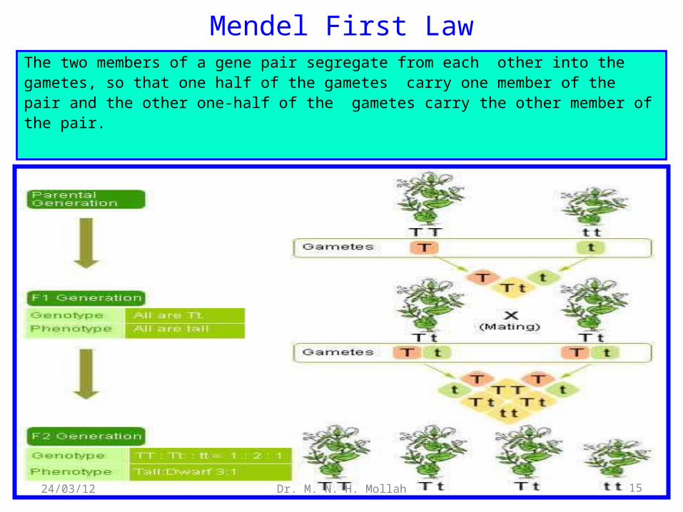
Mendel First LawThe two members of a gene pair segregate from each other into thegametes, so that one half of the gametes carry one member of the pair and the other one-half of the gametes carry the other member ofthe pair.
15Dr. M. N. H. Mollah24/03/12
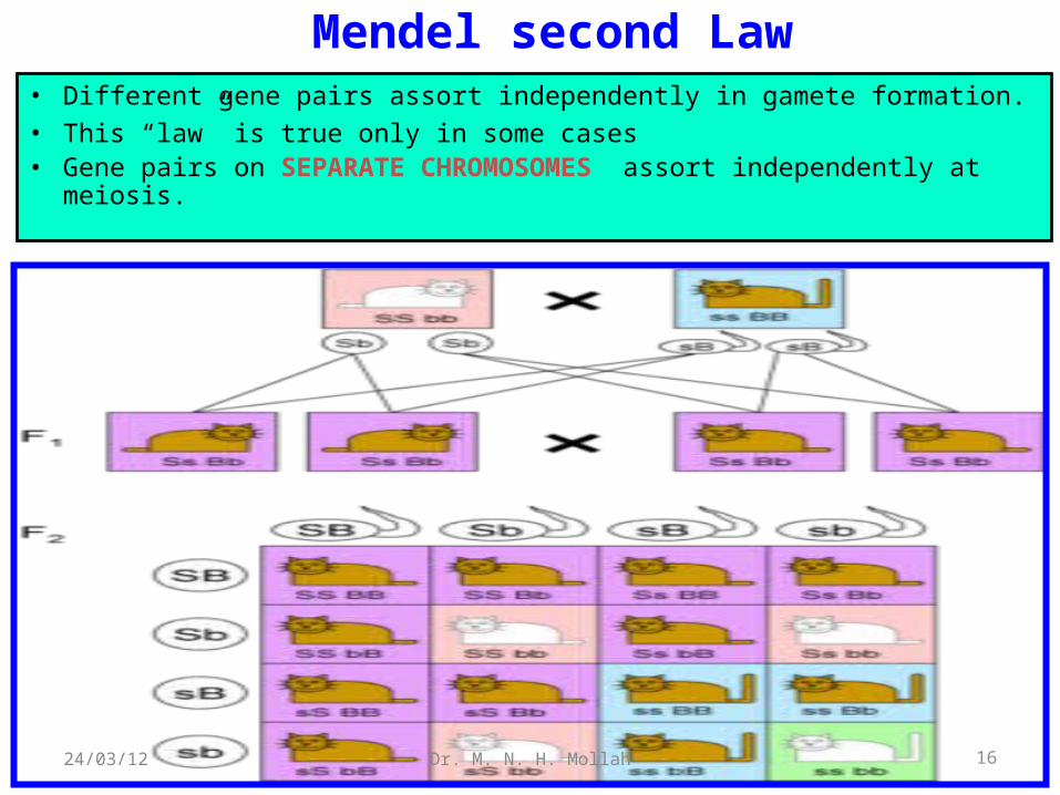
Mendel second Law• Different gene pairs assort independently in gamete formation.• This “law” is true only in some cases• Gene pairs on SEPARATE CHROMOSOMES assort
independently at meiosis.
16Dr. M. N. H. Mollah24/03/12
Linkage and MappingSyntenic & Nonsyntecnic: Loci on the same chromosome are
said to be syntenic, and those on different chromosomes are said to be nonsyntenic.
Linkage: The extent to which syntenic loci remain together depends on their closeness. We are thus led to consider the phenomenon of linkage.
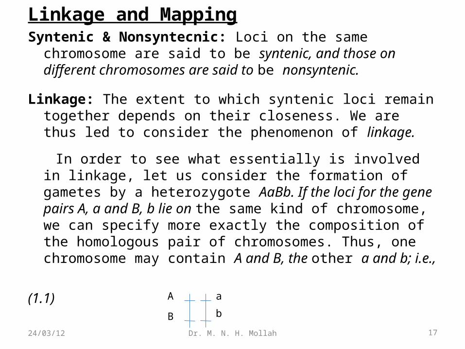
In order to see what essentially is involved in linkage, let us consider the formation of gametes by a heterozygote AaBb. If the loci for the gene pairs A, a and B, b lie on the same kind of chromosome, we can specify more exactly the composition of the homologous pair of chromosomes. Thus, one chromosome may contain A and B, the other a and b; i.e.,
(1.1)
aA
B b
17Dr. M. N. H. Mollah24/03/12
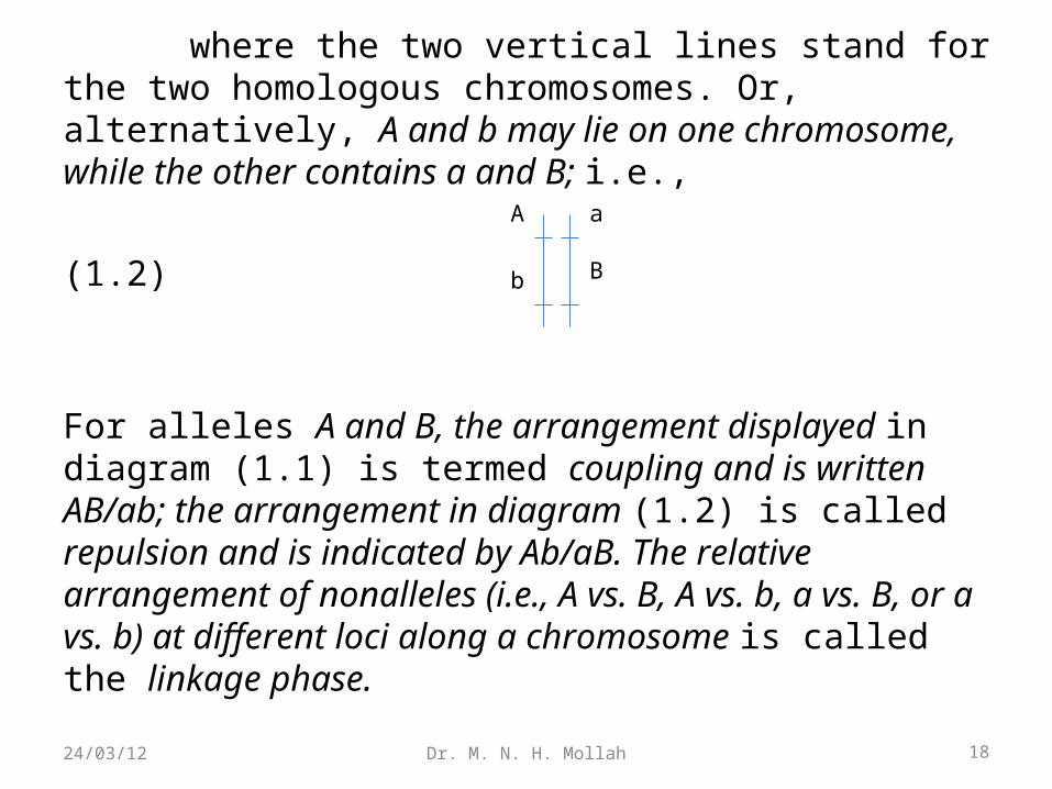
where the two vertical lines stand for the two homologous chromosomes. Or, alternatively, A and b may lie on one chromosome, while the other contains a and B; i.e.,
(1.2)
For alleles A and B, the arrangement displayed in diagram (1.1) is termed coupling and is written AB/ab; the arrangement in diagram (1.2) is called repulsion and is indicated by Ab/aB. The relative arrangement of nonalleles (i.e., A vs. B, A vs. b, a vs. B, or a vs. b) at different loci along a chromosome is called the linkage phase.
aA
b B
18Dr. M. N. H. Mollah24/03/12
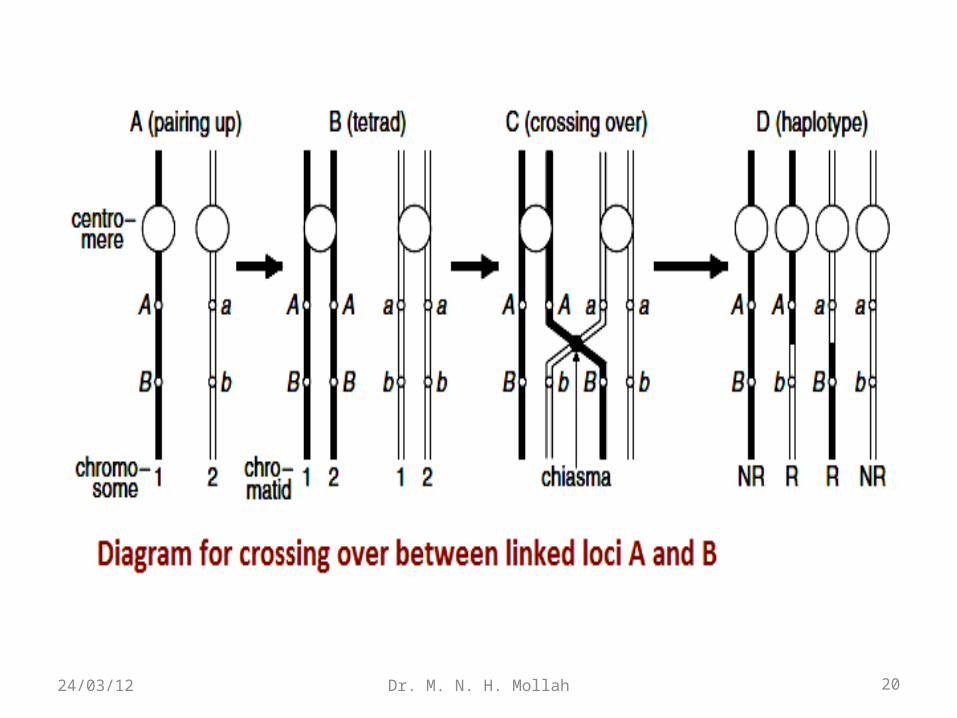
Crossing−over between linked loci A and BAt an early stage of meiosis, the two chromosomes 1 and 2 lie
side by side with corresponding loci aligned. If the parental genotype is AB/ab, we can represent the alignment as in Fig. 1.3A. Each of the paired chromosomes is then duplicated to form two sister strands (chromatids) connected to each other at a region called the centromere.
The homologous chromosomes form pairs, so that each resulting complex consists of four chromatids known as a tetrad (Fig. 1.3B). At this stage, the nonsister chromatids adhere to each other in a semi-random fashion at regions called chiasmata.
Each chiasma represents a point where crossing over between two nonsister chromatids can occur (Fig. 1.3C). Chiasmata do not occur entirely at random, as they are more likely farther away from the centromere, and it is unusual to find two chiasmata in very close proximity to each other.
19Dr. M. N. H. Mollah24/03/12
20Dr. M. N. H. Mollah24/03/12
Map Distance• The map distance between any two loci is the average number of
points of exchange occurring in the segment.
• For Example, One linkage map unit (LMU) is 1% recombination. Thus, the linkage map distance between two genes is the percentage recombination between those genes.
• In this case, we have a total of 300 recombinant offspring, out of 2000 total offspring. Map distance is calculated as (# Recombinants)/(Total offspring) X 100. So our map distance is (300/2000)x100, or 15 LMU.
21Dr. M. N. H. Mollah24/03/12
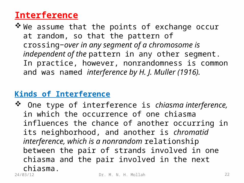
Interference We assume that the points of exchange occur at random, so
that the pattern of crossing−over in any segment of a chromosome is independent of the pattern in any other segment. In practice, however, nonrandomness is common and was named interference by H. J. Muller (1916).
Kinds of Interference One type of interference is chiasma interference, in which the
occurrence of one chiasma influences the chance of another occurring in its neighborhood, and another is chromatid interference, which is a nonrandom relationship between the pair of strands involved in one chiasma and the pair involved in the next chiasma.
22Dr. M. N. H. Mollah24/03/12
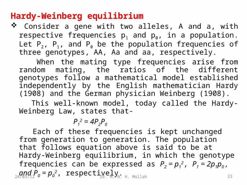
Hardy-Weinberg equilibrium Consider a gene with two alleles, A and a, with respective
frequencies p1 and p0, in a population. Let P2, P1, and P0 be the population frequencies of three genotypes, AA, Aa and aa, respectively.
When the mating type frequencies arise from random mating, the ratios of the different genotypes follow a mathematical model established independently by the English mathematician Hardy (1908) and the German physician Weinberg (1908).
This well-known model, today called the Hardy-Weinberg Law, states that-
P12 = 4P2P0
Each of these frequencies is kept unchanged from generation to generation. The population that follows equation above is said to be at Hardy-Weinberg equilibrium, in which the genotype frequencies can be expressed as P2 = p1
2, P1 = 2p1p0 , and P0 = p0
2, respectively. 23Dr. M. N. H. Mollah24/03/12
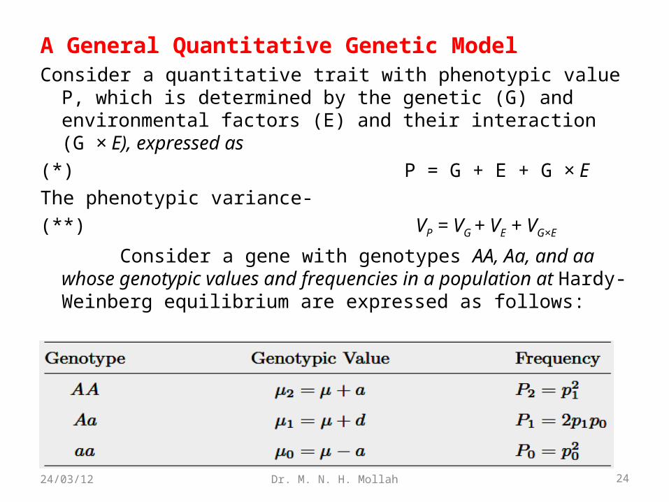
A General Quantitative Genetic ModelConsider a quantitative trait with phenotypic value P, which is
determined by the genetic (G) and environmental factors (E) and their interaction (G × E), expressed as
(*) P = G + E + G × E
The phenotypic variance-
(**) VP = VG + VE + VG×E
Consider a gene with genotypes AA, Aa, and aa whose genotypic values and frequencies in a population at Hardy-Weinberg equilibrium are expressed as follows:
24Dr. M. N. H. Mollah24/03/12
Where, μ= the overall mean of the trait;
a=the additive effect;
d=the dominance effect;
• If there is no dominance, d = 0;
• If allele A is dominant over a, d is positive;
• And if allele a is dominant over A, d is negative.
• Dominance is complete if d is equal to +a or −a,
• And there is over dominance if d is greater than +a or less than −a.
• The degree of dominance is described by the ratio d/a.
25Dr. M. N. H. Mollah24/03/12
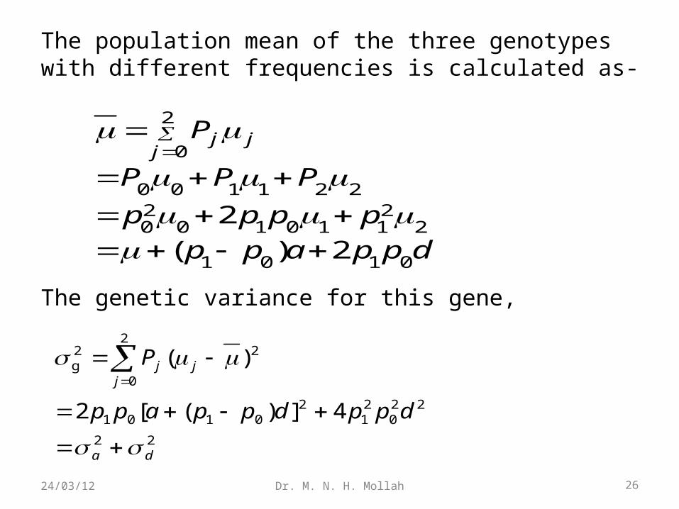
The population mean of the three genotypes with different frequencies is calculated as-
The genetic variance for this gene,
dppapp
pppp
PPP
Pj
jj
0101
2211010
20
221100
2
0
2)(
2
22
220
21
20101
2
0
22g
4])([2
)(
da
jjj
dppdppapp
P
26Dr. M. N. H. Mollah24/03/12
Where, α = a(p1 – p2)d is the average effect due to the substitution of alleles from A to a (Falconer and Mackay 1996).
Genetic Models for the Backcross and F2 Design Consider two parental populations, P1 and P2, fixed with favorable alleles A1, ...,Am and unfavorable alleles a1, ..., am, respectively, for all m loci.
The two parents are crossed to generate an F1. The F1 is backcrossed to one of the parents to form a backcross or self-crossed to form an F2.
Let ak and dk be the additive and dominance effects of gene k, respectively, and rkl be the recombination fraction between any two genes k and l.
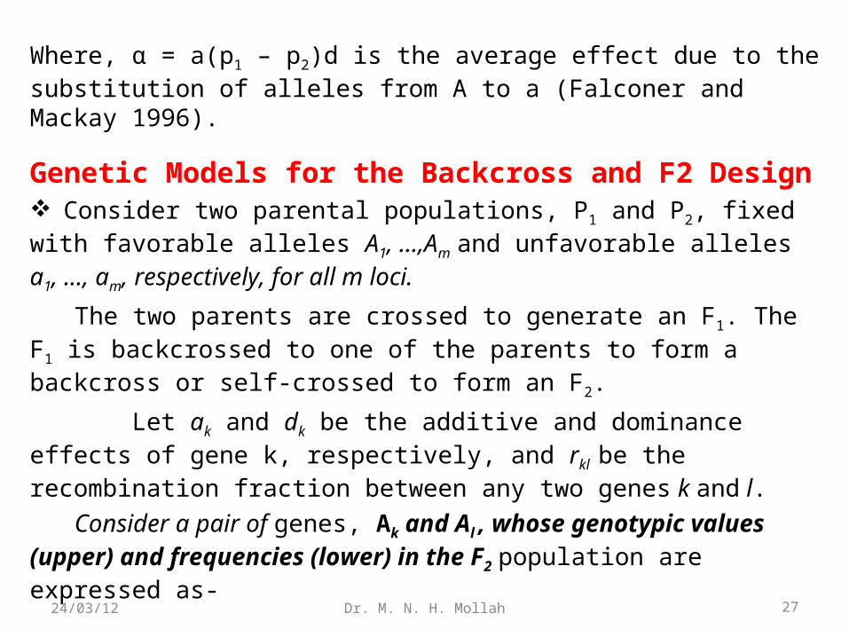
Consider a pair of genes, Ak and Al , whose genotypic values (upper) and frequencies (lower) in the F2 population are expressed as-
27Dr. M. N. H. Mollah24/03/12
where, the genotypic values are composed of the additive and dominance effects at the two genes.
28Dr. M. N. H. Mollah24/03/12
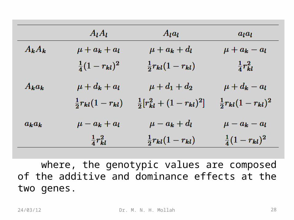
The genetic variance of the trait as-
• The first term on the right side of equation for the F2 is the additive variance within loci.
• The second is the dominance variance within loci. • The third is the additive covariance between different loci. • And the fourth is the dominance covariance between different
loci.
29Dr. M. N. H. Mollah24/03/12
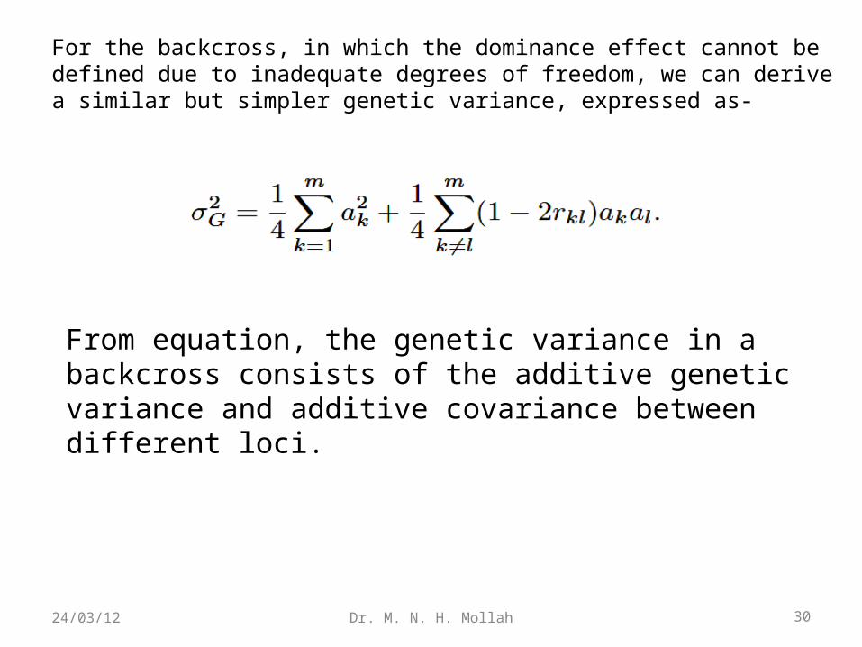
For the backcross, in which the dominance effect cannot be defined due to inadequate degrees of freedom, we can derive a similar but simpler genetic variance, expressed as-
From equation, the genetic variance in a backcross consists of the additive genetic variance and additive covariance between different loci.
30Dr. M. N. H. Mollah24/03/12
Epistatic Model The effect due to gene interaction was coined as epistasis by W.
Bateson (1902).
From a physiological perspective, epistasis describes the dependence of gene effects at one locus upon those at the other locus.
• Fisher (1918) first partitioned the genetic variance into additive, dominance, and epistatic components using the least squares principle.
• Cockerham (1954) further partitioned the two-gene epistatic variance into the additive × additive, additive × dominance, dominance × additive, and dominance × dominance interaction components.
31Dr. M. N. H. Mollah24/03/12
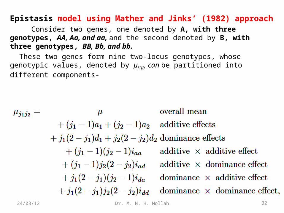
Epistasis model using Mather and Jinks’ (1982) approach Consider two genes, one denoted by A, with three genotypes, AA, Aa, and aa, and the second denoted by B, with three genotypes, BB, Bb, and bb.
These two genes form nine two-locus genotypes, whose genotypic values, denoted by μj1j2, can be partitioned into different components-
32Dr. M. N. H. Mollah24/03/12
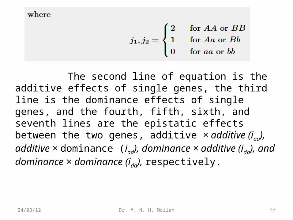
The second line of equation is the additive effects of single genes, the third line is the dominance effects of single genes, and the fourth, fifth, sixth, and seventh lines are the epistatic effects between the two genes, additive × additive (iaa), additive × dominance (iad), dominance × additive (ida), and dominance × dominance (idd), respectively.
33Dr. M. N. H. Mollah24/03/12
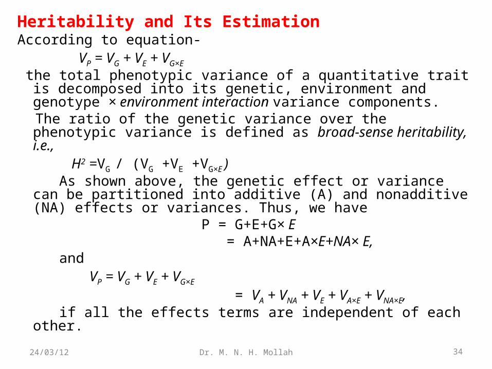
Heritability and Its EstimationAccording to equation- VP = VG + VE + VG×E
the total phenotypic variance of a quantitative trait is decomposed into its genetic, environment and genotype × environment interaction variance components.
The ratio of the genetic variance over the phenotypic variance is defined as broad-sense heritability, i.e.,
H2 =VG / (VG +VE +VG×E ) As shown above, the genetic effect or variance can be partitioned
into additive (A) and nonadditive (NA) effects or variances. Thus, we have
P = G+E+G× E = A+NA+E+A×E+NA× E, and VP = VG + VE + VG×E
= VA + VNA + VE + VA×E + VNA×E, if all the effects terms are independent of each other. 34Dr. M. N. H. Mollah24/03/12
(2) Linkage Analysis and Map Construction2.1 Introduction2.2 Experimental Design2.3 Mendelian Segregation 2.3.1 Testing Marker Segregation Patterns
2.4 Two-Point Analysis 2.4.1 Double Backcross 2.4.2 Double Intercross–F2
2.5 Three-Point Analysis2.6 Multilocus Likelihood and Locus Ordering2.7 Estimation with Many Loci2.8 Mixture Likelihoods and Order Probabilities
2.9 Map Functions 2.9.1 Mather’s Formula 2.9.2 The Morgan Map Function 2.9.3 The Haldane Map Function 2.9.4 The Kosambi Map Function
35Dr. M. N. H. Mollah24/03/12
2.1 IntroductionLinkage is the tendency for genes to be inherited together because they are located near
one another on the same chromosome. Linkage analysis of markers lays a foundation
for the construction of a genetic linkage map and the subsequent molecular dissection
of quantitative traits using the map. Linkage analysis is based on the cosegregation of
adjacent markers and their cotransmission to the next progeny generation.
The linkage of markers can be measured in terms of their recombination fraction or
genetic distance. The function of linkage analysis is to detect the relative locations of
two or more markers on the same chromosome. Linkage analysis can be performed for
a pair of markers (two-point analysis) or three markers simultaneously (three point
analysis). Two- or three-point analyses provide fundamental information for he
construction of a genetic linkage map that cover partly or entirely the genome.
The map function that converts the recombination fraction to genetic distance can be
derived from three-point analysis. Different forms of the map function are available that
depend on the assumption about the presence or absence of the interference of
crossovers between adjacent marker intervals. 36Dr. M. N. H. Mollah24/03/12
2.2 Experimental Design
Consider two inbred lines that are homologous for two alternative alleles
of each gene are crossed as parents P1 and P2 to generate an F1 progeny.
Thus, all F1 individuals are heterozygous at all genes.
These heterozygous F1’s can either be backcrossed to each of their
parents to generate two backcrosses (B1 and B2) or the F1 individuals can
be crossed with each other to produce the F2 generation.
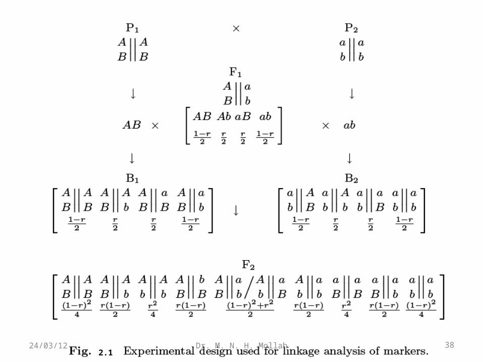
A diagram illustrating this crossing procedure is illustrated in Fig. 2.1.
Consider two markers, A, with alleles A and a, and B, with two alleles B
and b.
Two inbred line parents, P1 and P2, are homozygous for the large and
small alleles of these two genes, respectively. 37Dr. M. N. H. Mollah24/03/12
2.138Dr. M. N. H. Mollah24/03/12
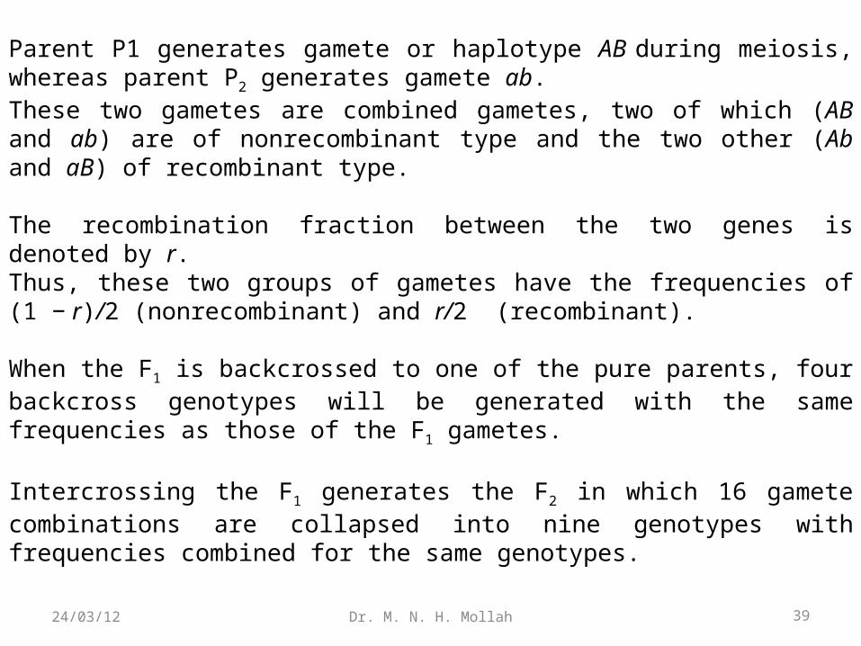
Parent P1 generates gamete or haplotype AB during meiosis, whereas parent P2 generates gamete ab. These two gametes are combined gametes, two of which (AB and ab) are of nonrecombinant type and the two other (Ab and aB) of recombinant type.
The recombination fraction between the two genes is denoted by r. Thus, these two groups of gametes have the frequencies of (1 − r)/2 (nonrecombinant) and r/2 (recombinant).
When the F1 is backcrossed to one of the pure parents, four backcross genotypes will be generated with the same frequencies as those of the F1 gametes.
Intercrossing the F1 generates the F2 in which 16 gamete combinations are collapsed into nine genotypes with frequencies combined for the same genotypes.
39Dr. M. N. H. Mollah24/03/12
2.3 Mendelian Segregation
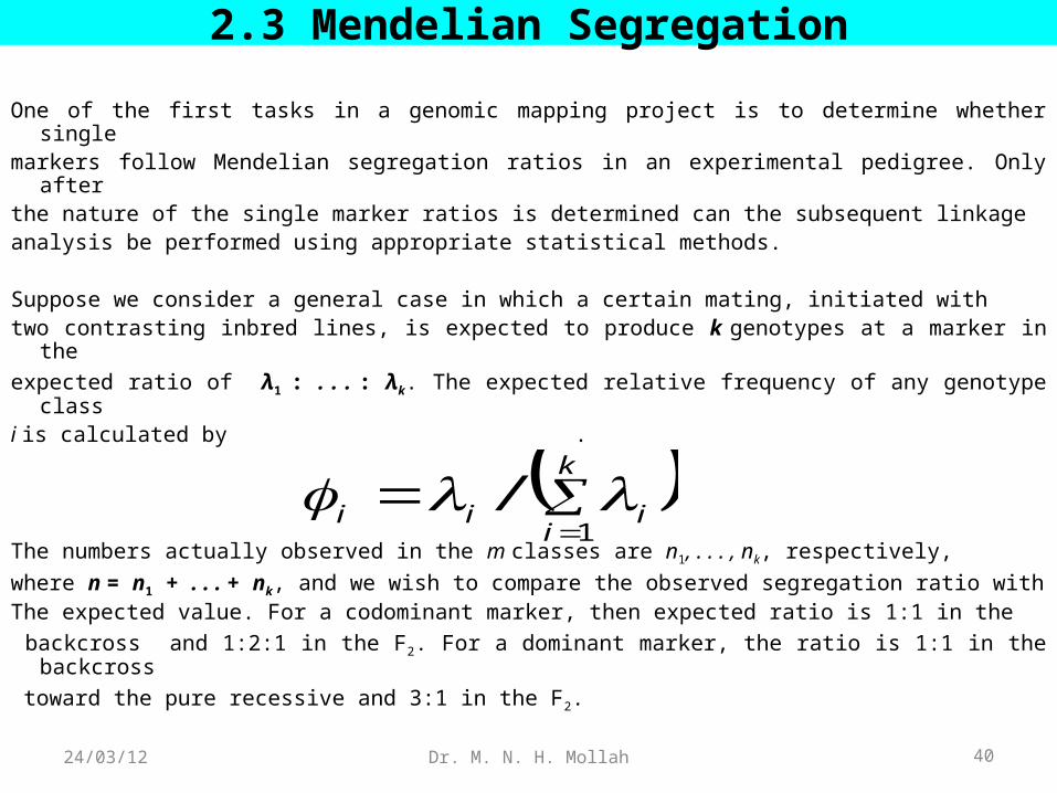
One of the first tasks in a genomic mapping project is to determine whether singlemarkers follow Mendelian segregation ratios in an experimental pedigree. Only afterthe nature of the single marker ratios is determined can the subsequent linkageanalysis be performed using appropriate statistical methods.
Suppose we consider a general case in which a certain mating, initiated withtwo contrasting inbred lines, is expected to produce k genotypes at a marker in the
expected ratio of λ1 : . . . : λk. The expected relative frequency of any genotype classi is calculated by .
The numbers actually observed in the m classes are n1, . . . , nk, respectively,
where n = n1 + . . . + nk, and we wish to compare the observed segregation ratio withThe expected value. For a codominant marker, then expected ratio is 1:1 in the
backcross and 1:2:1 in the F2. For a dominant marker, the ratio is 1:1 in the backcross
toward the pure recessive and 3:1 in the F2.
k
iiii /
1
40Dr. M. N. H. Mollah24/03/12
2.3.1 Testing Marker Segregation Patterns
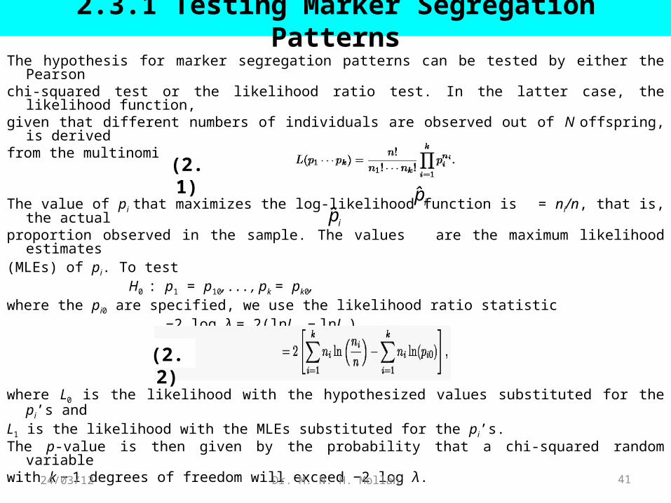
The hypothesis for marker segregation patterns can be tested by either the Pearsonchi-squared test or the likelihood ratio test. In the latter case, the likelihood function,given that different numbers of individuals are observed out of N offspring, is derivedfrom the multinomial distribution and given by
The value of pi that maximizes the log-likelihood function is = ni/n, that is, the actualproportion observed in the sample. The values are the maximum likelihood estimates(MLEs) of pi. To test H0 : p1 = p10, . . . , pk = pk0,where the pi0 are specified, we use the likelihood ratio statistic −2 log λ = 2(lnL1 − lnL0)
where L0 is the likelihood with the hypothesized values substituted for the pi’s andL1 is the likelihood with the MLEs substituted for the pi’s.The p-value is then given by the probability that a chi-squared random variablewith k − 1 degrees of freedom will exceed −2 log λ.
ip̂ip̂
(2.1)
(2.2)
41Dr. M. N. H. Mollah24/03/12
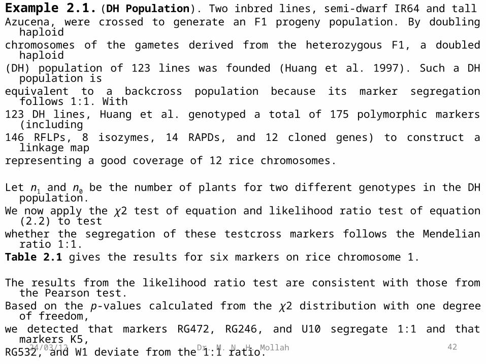
Example 2.1. (DH Population). Two inbred lines, semi-dwarf IR64 and tallAzucena, were crossed to generate an F1 progeny population. By doubling haploidchromosomes of the gametes derived from the heterozygous F1, a doubled haploid(DH) population of 123 lines was founded (Huang et al. 1997). Such a DH population
isequivalent to a backcross population because its marker segregation follows 1:1. With123 DH lines, Huang et al. genotyped a total of 175 polymorphic markers (including146 RFLPs, 8 isozymes, 14 RAPDs, and 12 cloned genes) to construct a linkage maprepresenting a good coverage of 12 rice chromosomes.
Let n1 and n0 be the number of plants for two different genotypes in the DH population.We now apply the χ2 test of equation and likelihood ratio test of equation (2.2) to testwhether the segregation of these testcross markers follows the Mendelian ratio 1:1.Table 2.1 gives the results for six markers on rice chromosome 1.
The results from the likelihood ratio test are consistent with those from the Pearson test.
Based on the p-values calculated from the χ2 distribution with one degree of freedom,we detected that markers RG472, RG246, and U10 segregate 1:1 and that markers K5,RG532, and W1 deviate from the 1:1 ratio.
42Dr. M. N. H. Mollah24/03/12
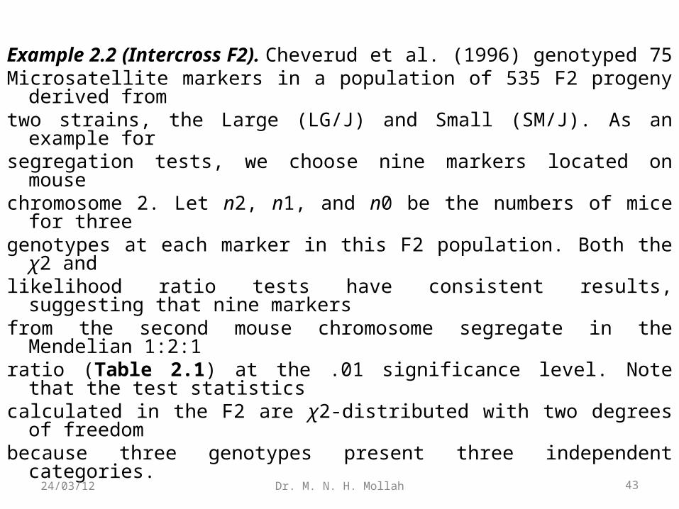
Example 2.2 (Intercross F2). Cheverud et al. (1996) genotyped 75 Microsatellite markers in a population of 535 F2 progeny derived from two strains, the Large (LG/J) and Small (SM/J). As an example for segregation tests, we choose nine markers located on mouse chromosome 2. Let n2, n1, and n0 be the numbers of mice for three genotypes at each marker in this F2 population. Both the χ2 andlikelihood ratio tests have consistent results, suggesting that nine
markers from the second mouse chromosome segregate in the Mendelian 1:2:1 ratio (Table 2.1) at the .01 significance level. Note that the test statistics calculated in the F2 are χ2-distributed with two degrees of freedom because three genotypes present three independent categories.
43Dr. M. N. H. Mollah24/03/12
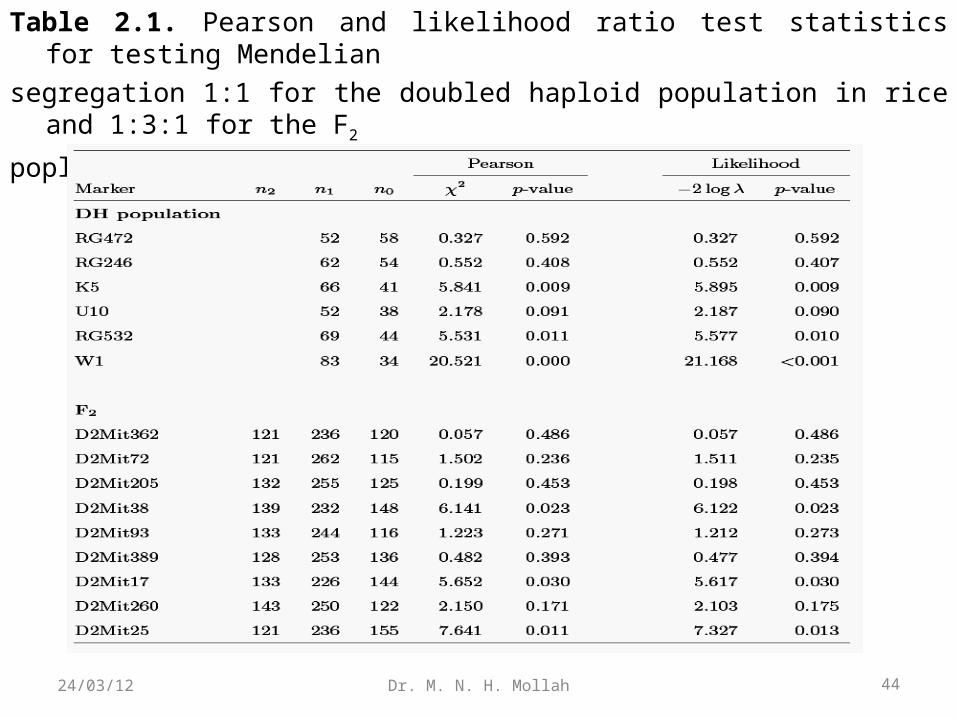
Table 2.1. Pearson and likelihood ratio test statistics for testing Mendelian
segregation 1:1 for the doubled haploid population in rice and 1:3:1 for the F2
poplation in mice.
44Dr. M. N. H. Mollah24/03/12
2.4 Two-Point Analysis
● Two-point analysis is a statistical approach for estimating
and testing the recombination fraction between two different
markers.
● Two-point analysis provides a basis for the derivation of the map function and the construction of genetic linkage maps.
Here, we will present statistical methods for linkage analysis
separately for the backcross and F2 populations, because these
types of populations need different analytical strategies.
45Dr. M. N. H. Mollah24/03/12
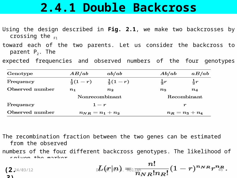
2.4.1 Double Backcross
Using the design described in Fig. 2.1, we make two backcrosses by crossing the F1
toward each of the two parents. Let us consider the backcross to parent P2. The
expected frequencies and observed numbers of the four genotypes generated in this
backcross can be tabulated as follows:
The recombination fraction between the two genes can be estimated from the observed
numbers of the four different backcross genotypes. The likelihood of r given the marker
data n = (nNR, nR) is
(2.3) 46Dr. M. N. H. Mollah24/03/12
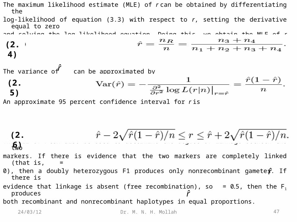
The maximum likelihood estimate (MLE) of r can be obtained by differentiating thelog-likelihood of equation (3.3) with respect to r, setting the derivative equal to zeroand solving the log-likelihood equation. Doing this, we obtain the MLE of r as
The variance of can be approximated by
An approximate 95 percent confidence interval for r is
The MLE of r can also be used to determine the degree of linkage between the twomarkers. If there is evidence that the two markers are completely linked (that is, =0), then a doubly heterozygous F1 produces only nonrecombinant gametes. If there is
evidence that linkage is absent (free recombination), so = 0.5, then the F1 producesboth recombinant and nonrecombinant haplotypes in equal proportions.
r̂
r̂
r̂
(2.4)
(2.5)
(2.6)
47Dr. M. N. H. Mollah24/03/12
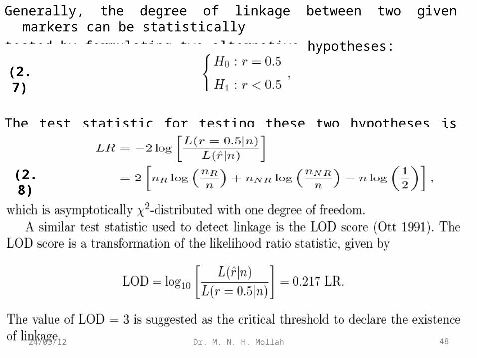
Generally, the degree of linkage between two given markers can be statistically
tested by formulating two alternative hypotheses:
The test statistic for testing these two hypotheses is the log-likelihood ratio (LR):
(2.7)
(2.8)
48Dr. M. N. H. Mollah24/03/12
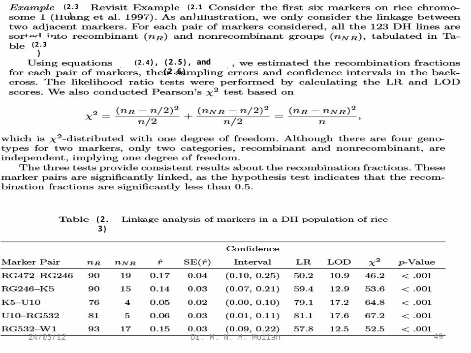
(2.3) (2.1)
(2.3)
(2.4), (2.5), and (2.6)
(2.3)
49Dr. M. N. H. Mollah24/03/12
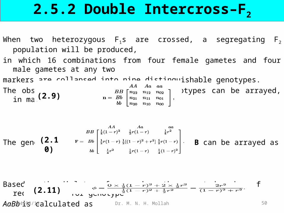
2.5.2 Double Intercross–F2
When two heterozygous F1s are crossed, a segregating F2 population will be produced,
in which 16 combinations from four female gametes and four male gametes at any two
markers are collapsed into nine distinguishable genotypes.
The observed numbers of these nine genotypes can be arrayed, in matrix notation, as
The genotype frequencies for markers A and B can be arrayed as
Based on the diplotype frequencies, the expected number of recombinants for genotype
AaBb is calculated as
(2.9)
(2.10)
(2.11)
50Dr. M. N. H. Mollah24/03/12
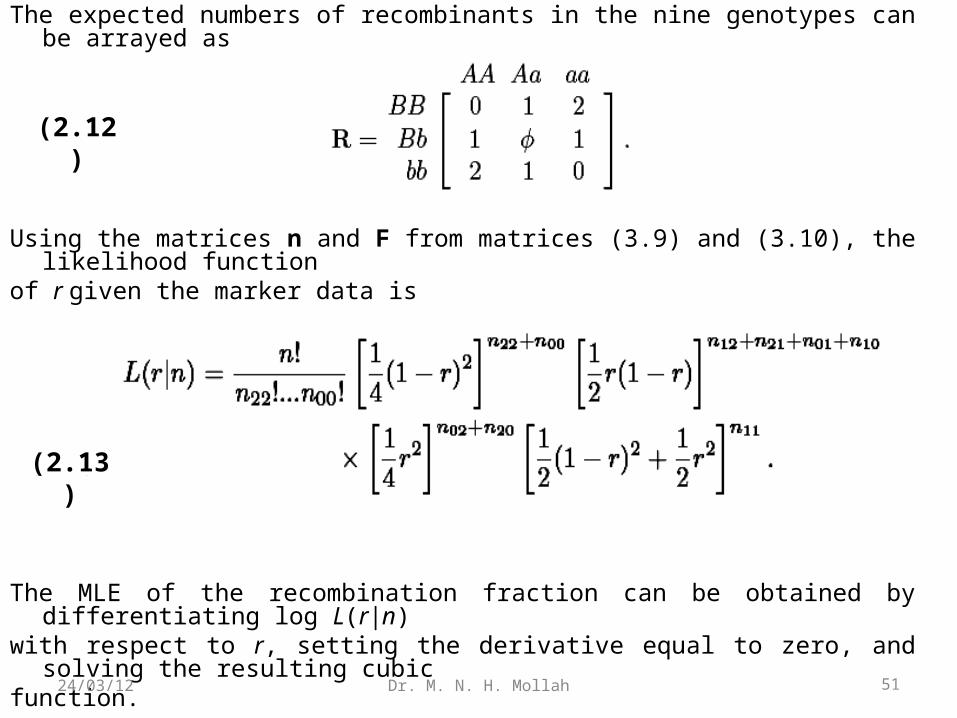
The expected numbers of recombinants in the nine genotypes can be arrayed as
Using the matrices n and F from matrices (3.9) and (3.10), the likelihood functionof r given the marker data is
The MLE of the recombination fraction can be obtained by differentiating log L(r|n)with respect to r, setting the derivative equal to zero, and solving the resulting cubicfunction.
(2.12)
(2.13)
51Dr. M. N. H. Mollah24/03/12
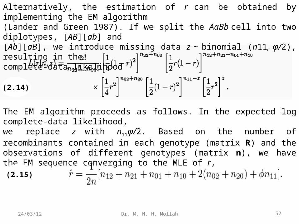
The EM algorithm proceeds as follows. In the expected log complete-data likelihood,we replace z with n11φ/2. Based on the number of recombinants contained in each genotype (matrix R) and the observations of different genotypes (matrix n), we have the EM sequence converging to the MLE of r,
Alternatively, the estimation of r can be obtained by implementing the EM algorithm(Lander and Green 1987). If we split the AaBb cell into two diplotypes, [AB][ab] and[Ab][aB], we introduce missing data z ∼ binomial (n11, φ/2), resulting in thecomplete-data likelihood
(2.14)
(2.15)
52Dr. M. N. H. Mollah24/03/12
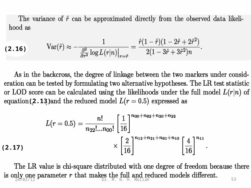
(2.16)
(2.17)
(2.13)
53Dr. M. N. H. Mollah24/03/12
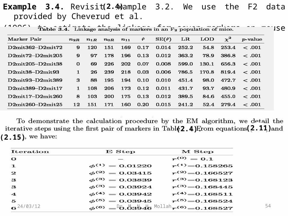
Example 3.4. Revisit Example 3.2. We use the F2 data provided by Cheverud et al.
(1996) to estimate the linkage for seven markers on mouse chromosome 2.
(2.4)
(2.4). (2.11)(2.15)
54Dr. M. N. H. Mollah24/03/12
2.5 Three-Point AnalysisCompared with a two-point analysis, a three-point analysis has two advantages: (1) It may increase the precision of the estimates of the recombination fractions when markers are not fully informative and (2) it provides a way of determining the optimalorder of different markers.
Consider three markers, A, B, and C, without a particular order for a triply heterozygous F1, from which a triple backcross or F2 is generated.
Let us first consider a backcross ABC/abc × abc/abc. A total of eight groups of markergenotypes in the backcross progeny can be classified into four groups based on thenumber of recombinants between marker pair A and B and between marker pair B andC.
These four groups are genotypes AbC/abc and aBc/abc (one recombinant from eachpair), Abc/abc and aBc/abc (one recombinant only from the first pair), ABc/abc andabC/abc (one recombinant only from the second pair), and ABC/abc and abc/abc (norecombinant for each pair).
55Dr. M. N. H. Mollah24/03/12
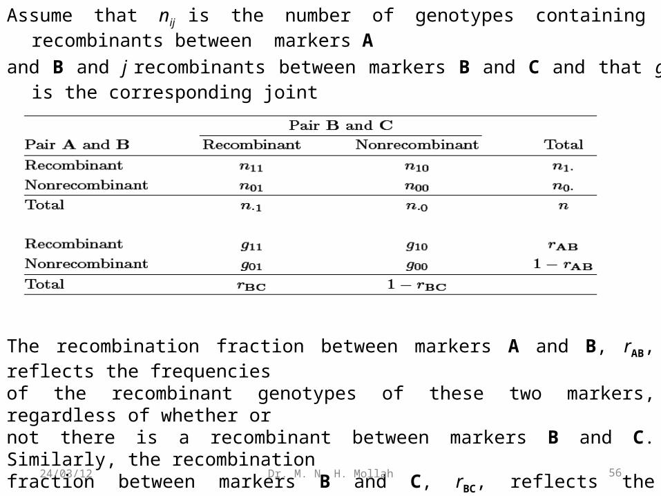
Assume that nij is the number of genotypes containing i recombinants between markers A
and B and j recombinants between markers B and C and that gij is the corresponding joint
recombination fraction. Both nij and gij can be expressed as
The recombination fraction between markers A and B, rAB, reflects the frequenciesof the recombinant genotypes of these two markers, regardless of whether ornot there is a recombinant between markers B and C. Similarly, the recombinationfraction between markers B and C, rBC, reflects the frequencies of the recombinantgenotypes of these two markers, regardless of the types of genotypes between markersA and B.
56Dr. M. N. H. Mollah24/03/12
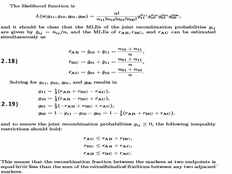
(2.19)
(2.18)
57Dr. M. N. H. Mollah24/03/12
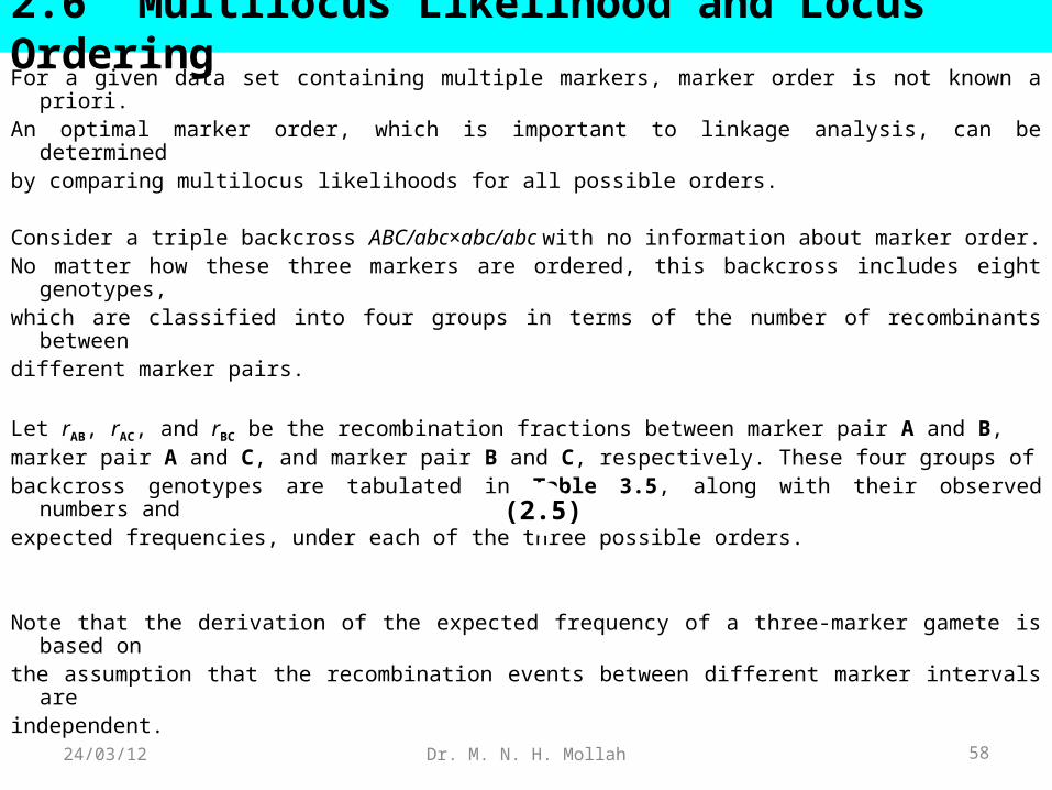
2.6 Multilocus Likelihood and Locus OrderingFor a given data set containing multiple markers, marker order is not known a priori.An optimal marker order, which is important to linkage analysis, can be determinedby comparing multilocus likelihoods for all possible orders.
Consider a triple backcross ABC/abc×abc/abc with no information about marker order.No matter how these three markers are ordered, this backcross includes eight
genotypes,which are classified into four groups in terms of the number of recombinants betweendifferent marker pairs.
Let rAB, rAC, and rBC be the recombination fractions between marker pair A and B,marker pair A and C, and marker pair B and C, respectively. These four groups ofbackcross genotypes are tabulated in Table 3.5, along with their observed numbers andexpected frequencies, under each of the three possible orders.
Note that the derivation of the expected frequency of a three-marker gamete is based onthe assumption that the recombination events between different marker intervals areindependent.
(2.5)
58Dr. M. N. H. Mollah24/03/12
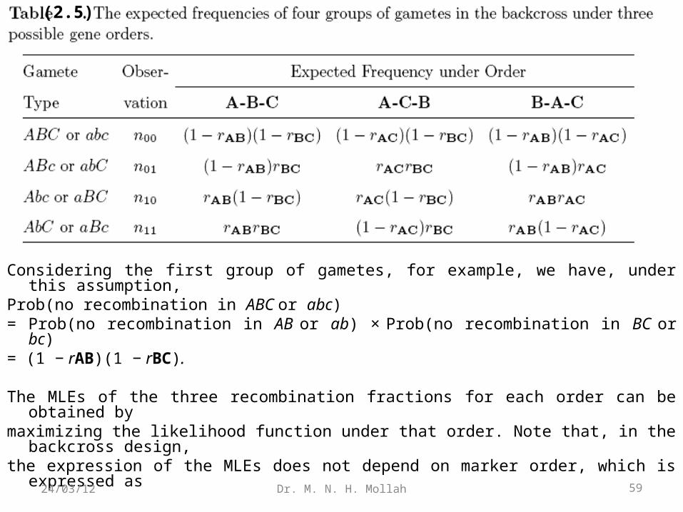
Considering the first group of gametes, for example, we have, under this assumption,Prob(no recombination in ABC or abc)= Prob(no recombination in AB or ab) × Prob(no recombination in BC or bc)= (1 − rAB)(1 − rBC).
The MLEs of the three recombination fractions for each order can be obtained bymaximizing the likelihood function under that order. Note that, in the backcross design,the expression of the MLEs does not depend on marker order, which is expressed as
(2.5)
59Dr. M. N. H. Mollah24/03/12
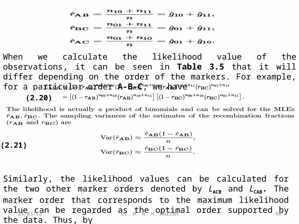
When we calculate the likelihood value of the observations, it can be seen in Table 3.5 that it will differ depending on the order of the markers. For example, for a particular order A-B-C, we have
Similarly, the likelihood values can be calculated for the two other marker orders denoted by LACB and LCAB. The marker order that corresponds to the maximum likelihood value can be regarded as the optimal order supported by the data. Thus, bycomparing the three likelihood values, LABC, LACB, and LCAB, we can determine the most likely marker order.
(2.20)
(2.21)
60Dr. M. N. H. Mollah24/03/12
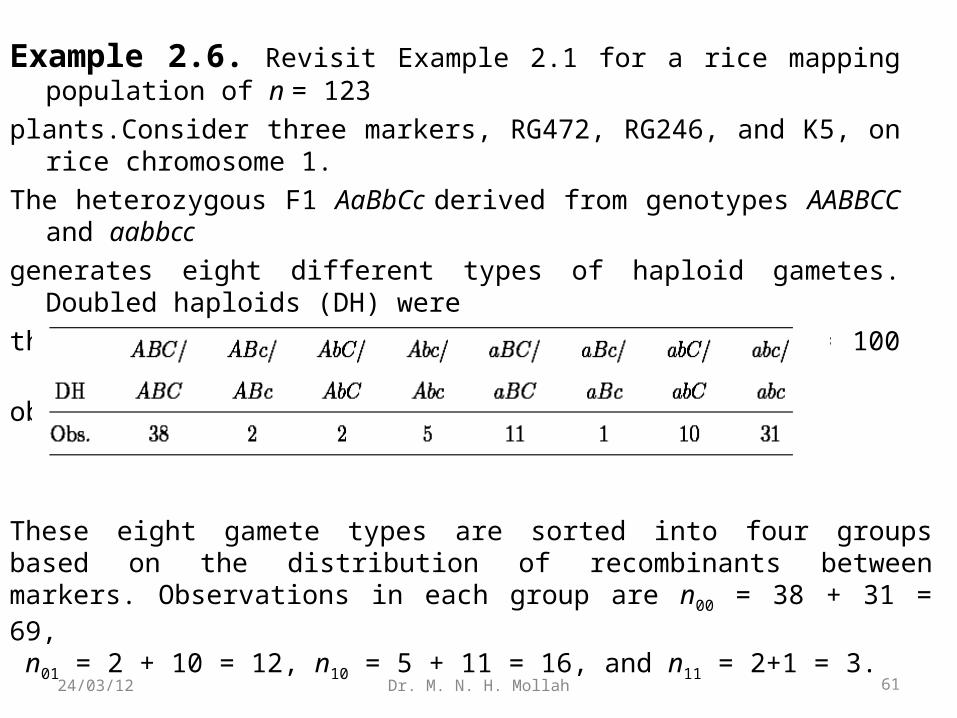
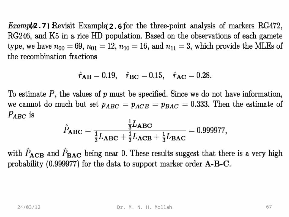
Example 2.6. Revisit Example 2.1 for a rice mapping population of n = 123
plants.Consider three markers, RG472, RG246, and K5, on rice chromosome 1.
The heterozygous F1 AaBbCc derived from genotypes AABBCC and aabbcc
generates eight different types of haploid gametes. Doubled haploids (DH) were
then observed for each gamete type as follows (n = 100 after deleting the
observations missing in the three markers):
These eight gamete types are sorted into four groups based on the distribution of recombinants between markers. Observations in each group are n00 = 38 + 31 = 69, n01 = 2 + 10 = 12, n10 = 5 + 11 = 16, and n11 = 2+1 = 3.
61Dr. M. N. H. Mollah24/03/12
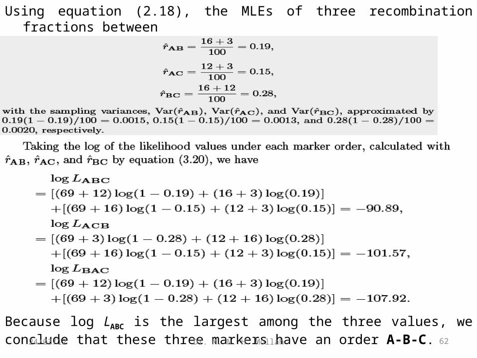
Using equation (2.18), the MLEs of three recombination fractions betweeneach pair of these three markers are estimated as
Because log LABC is the largest among the three values, we conclude that these three markers have an order A-B-C. 62Dr. M. N. H. Mollah24/03/12
In principle, the problems of locus ordering and interloci distance estimation can be
tackled simultaneously by comparing the likelihoods maximized over interloci distances
for all possible locus orders.
However, the number of possible orders, as well as the computer time and memory
required for each multilocus likelihood calculation, increases rapidly with the number
of loci.
There are two main approaches to the generation of approximate orders.
One approach is to start with a small number of markers whose order can be
established by a likelihood analysis and then proceed to place the remaining markers,
one at a time, into one of the intervals between the markers already in the map.
The second approach for generating approximate orders is to analyze all pairs of
loci using two-point linkage analysis and then subject the m(m−1)/2 recombination
fraction estimates (or maximum LOD scores) to some method of seriation.
2.7 Estimation with Many Loci
63Dr. M. N. H. Mollah24/03/12
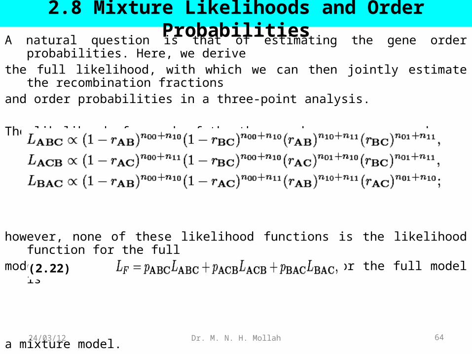
2.8 Mixture Likelihoods and Order ProbabilitiesA natural question is that of estimating the gene order probabilities. Here, we derivethe full likelihood, with which we can then jointly estimate the recombination fractionsand order probabilities in a three-point analysis.
The likelihoods for each of the three orders are expressed as
however, none of these likelihood functions is the likelihood function for the fullmodel for the data. The likelihood function for the full model is
a mixture model.
(2.22)
64Dr. M. N. H. Mollah24/03/12
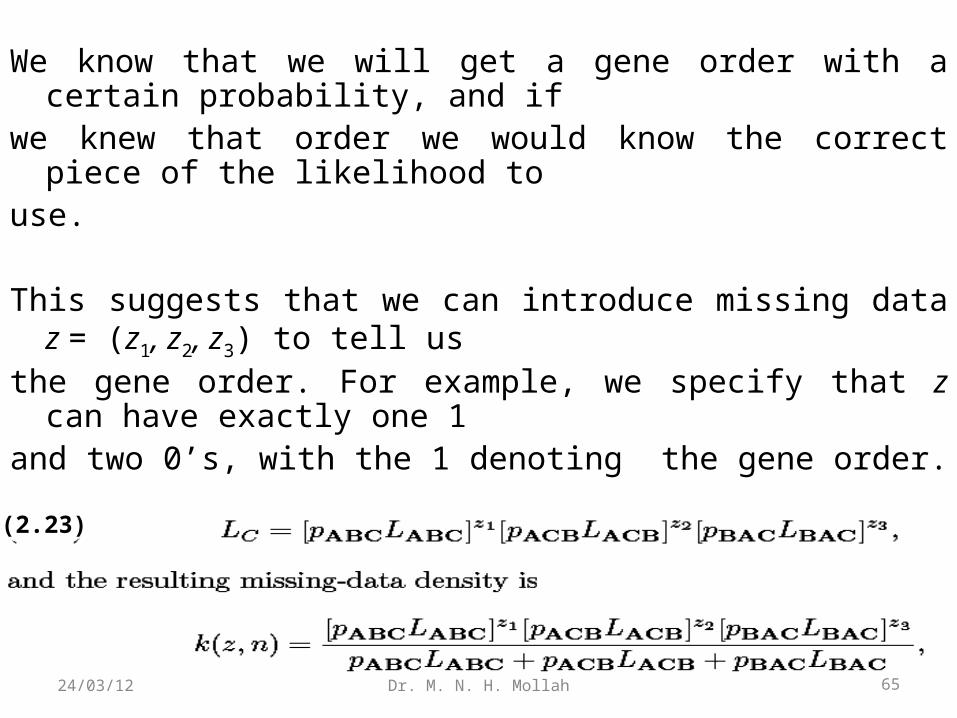
We know that we will get a gene order with a certain probability, and if we knew that order we would know the correct piece of the likelihood to use.
This suggests that we can introduce missing data z = (z1, z2, z3) to tell us the gene order. For example, we specify that z can have exactly one 1 and two 0’s, with the 1 denoting the gene order.
The joint complete-data likelihood of (n, z) is
(2.23)
65Dr. M. N. H. Mollah24/03/12
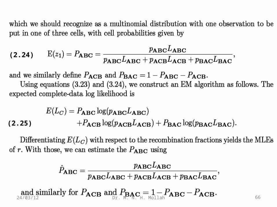
(2.24)
(2.25)
66Dr. M. N. H. Mollah24/03/12
(2.7): (2.6)
67Dr. M. N. H. Mollah24/03/12
Map Functions: The map function is a mathematical function that converts therecombination fraction (r) between two loci to the genetic distance separating them (d).The recombination fraction is not an additive distance measure.
Consider three markers A, B, and C. If the recombination fraction between markers Aand B and that between markers B and C are each assumed to be equal to r = 0.30, thenthe recombination fraction between markers A and C cannot be 2r since that valuewould exceed 50 percent. One therefore needs to transform the recombination fraction,r, into the additive map distance, d.
Map Distance: The map distance between the two loci is defined as the expectednumber of crossovers occurring between them on a single chromatid during meiosis.
The two nonalleles, each from a locus, will be derived from the same parentalchromosomes if no crossover or an even number of crossovers occurs between the twoloci, and from the different parental chromosomes if an odd number of crossoversoccurs between the two loci. Therefore, we can formulate a theoretical model toexpress the recombination fraction between two loci in terms of their map distanceor length by using the number of crossover events.
2.9 Map Functions & Distance
68Dr. M. N. H. Mollah24/03/12
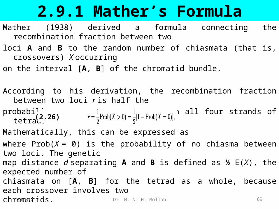
2.9.1 Mather’s FormulaMather (1938) derived a formula connecting the recombination fraction between two
loci A and B to the random number of chiasmata (that is, crossovers) X occurring
on the interval [A, B] of the chromatid bundle.
According to his derivation, the recombination fraction between two loci r is half the
probability of chiasmata occurring in all four strands of tetrads between the loci.
Mathematically, this can be expressed as
where Prob(X = 0) is the probability of no chiasma between two loci. The geneticmap distance d separating A and B is defined as ½ E(X), the expected number ofchiasmata on [A, B] for the tetrad as a whole, because each crossover involves twochromatids.
(2.26)
69Dr. M. N. H. Mollah24/03/12
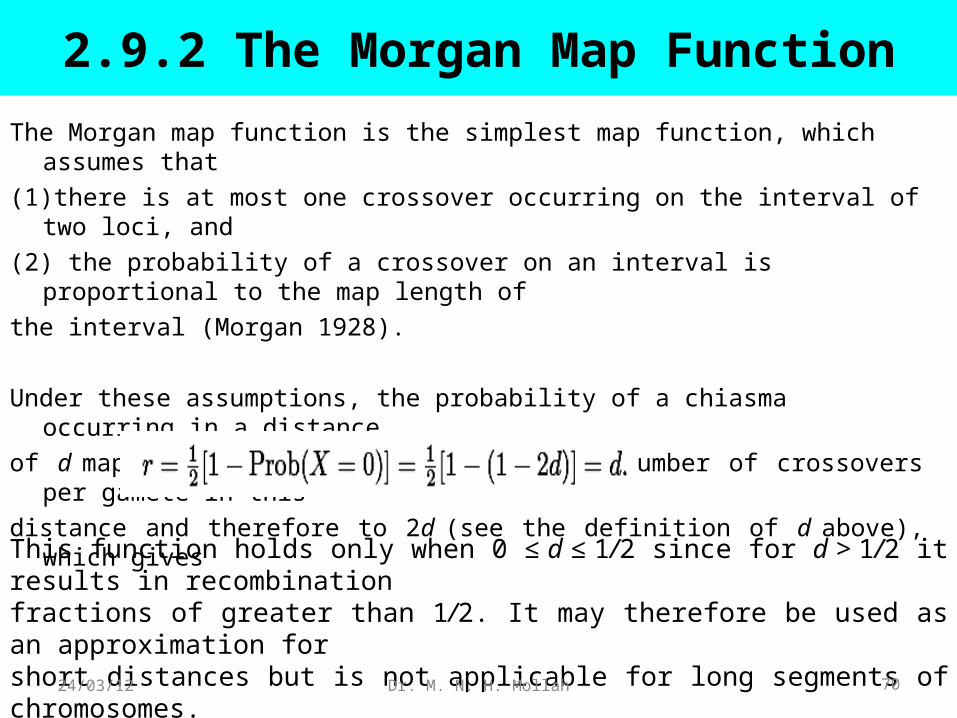
2.9.2 The Morgan Map Function
The Morgan map function is the simplest map function, which assumes that
(1)there is at most one crossover occurring on the interval of two loci, and
(2) the probability of a crossover on an interval is proportional to the map length of
the interval (Morgan 1928).
Under these assumptions, the probability of a chiasma occurring in a distance
of d map units is equal to the expected number of crossovers per gamete in this
distance and therefore to 2d (see the definition of d above), which gives
This function holds only when 0 ≤ d ≤ 1/2 since for d > 1/2 it results in recombinationfractions of greater than 1/2. It may therefore be used as an approximation forshort distances but is not applicable for long segments of chromosomes.
70Dr. M. N. H. Mollah24/03/12
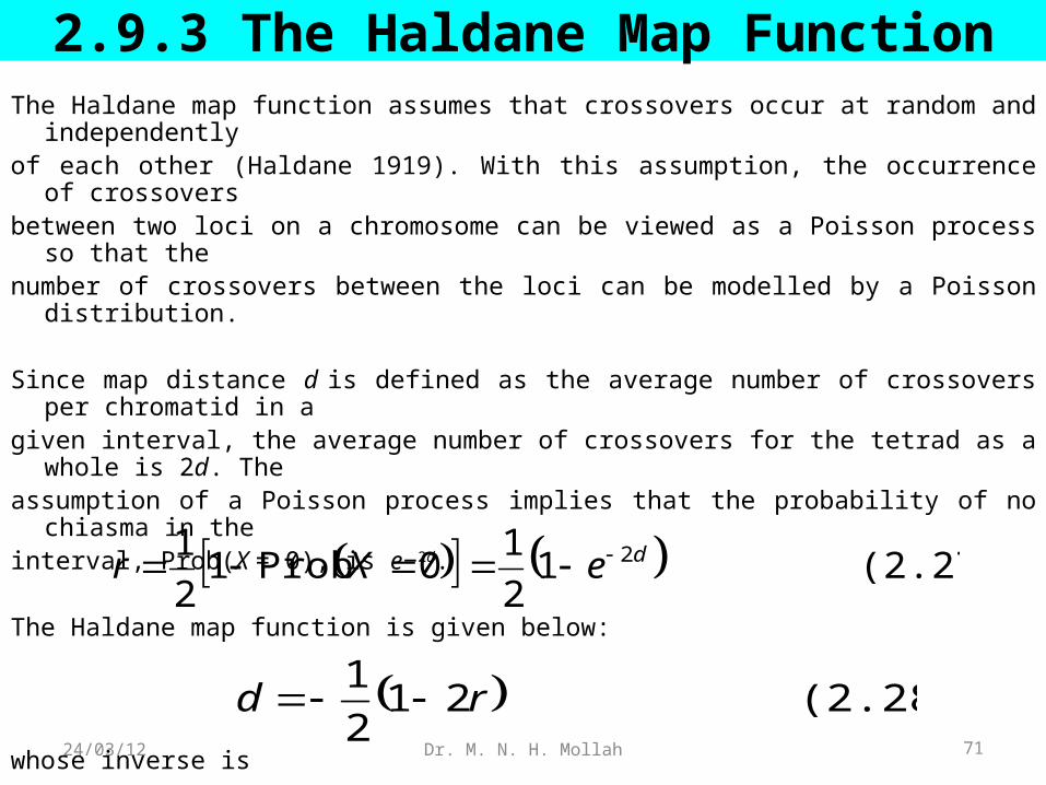
2.9.3 The Haldane Map FunctionThe Haldane map function assumes that crossovers occur at random and independentlyof each other (Haldane 1919). With this assumption, the occurrence of crossoversbetween two loci on a chromosome can be viewed as a Poisson process so that thenumber of crossovers between the loci can be modelled by a Poisson distribution.
Since map distance d is defined as the average number of crossovers per chromatid in agiven interval, the average number of crossovers for the tetrad as a whole is 2d. Theassumption of a Poisson process implies that the probability of no chiasma in theinterval, Prob(X = 0), is e−2d.
The Haldane map function is given below:
whose inverse is
(2.27)12
10Prob1
2
1 2deXr
(2.28)212
1rd
71Dr. M. N. H. Mollah24/03/12
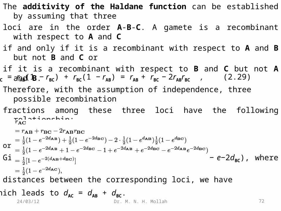
The additivity of the Haldane function can be established by assuming that three
loci are in the order A-B-C. A gamete is a recombinant with respect to A and C
if and only if it is a recombinant with respect to A and B but not B and C or
if it is a recombinant with respect to B and C but not A and B.
Therefore, with the assumption of independence, three possible recombination
fractions among these three loci have the following relationship:
or 1 − 2rAC = (1 − 2rAB)(1 − 2rBC).
Given rAB = 1/2 (1 − e−2dAB) and rBC = 1/2 (1 − e−2dBC), where the d’s are the map
distances between the corresponding loci, we have
rAC = rAB(1 − rBC) + rBC(1 − rAB) = rAB + rBC − 2rABrBC , (2.29)
which leads to dAC = dAB + dBC.72Dr. M. N. H. Mollah24/03/12
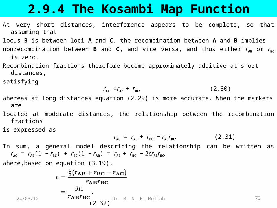
2.9.4 The Kosambi Map FunctionAt very short distances, interference appears to be complete, so that assuming that
locus B is between loci A and C, the recombination between A and B implies
nonrecombination between B and C, and vice versa, and thus either rAB or rBC is zero.
Recombination fractions therefore become approximately additive at short distances,
satisfying rAC =rAB + rBC, (2.30)
whereas at long distances equation (2.29) is more accurate. When the markers are
located at moderate distances, the relationship between the recombination fractions
is expressed as rAC = rAB + rBC − rABrBC. (2.31)
In sum, a general model describing the relationship can be written asrAC = rAB(1 − rBC) + rBC(1 − rAB) = rAB + rBC − 2crABrBC,
where,based on equation (3.19),
(2.32)73Dr. M. N. H. Mollah24/03/12
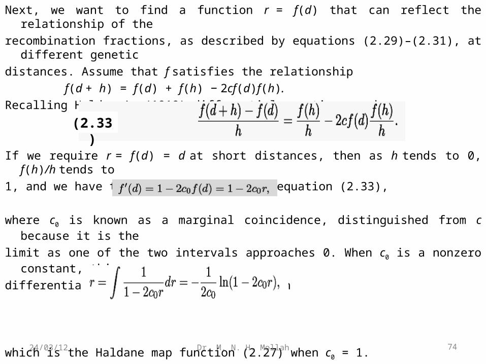
Next, we want to find a function r = f(d) that can reflect the relationship of the
recombination fractions, as described by equations (2.29)–(2.31), at different genetic
distances. Assume that f satisfies the relationship
f(d + h) = f(d) + f(h) − 2cf(d)f(h).
Recalling Haldane’s (1919) differential equation, we have
If we require r = f(d) = d at short distances, then as h tends to 0, f(h)/h tends to
1, and we have the derivative based on equation (2.33),
where c0 is known as a marginal coincidence, distinguished from c because it is the
limit as one of the two intervals approaches 0. When c0 is a nonzero constant, this
differential equation yields the solution
which is the Haldane map function (2.27) when c0 = 1.
(2.33)
74Dr. M. N. H. Mollah24/03/12
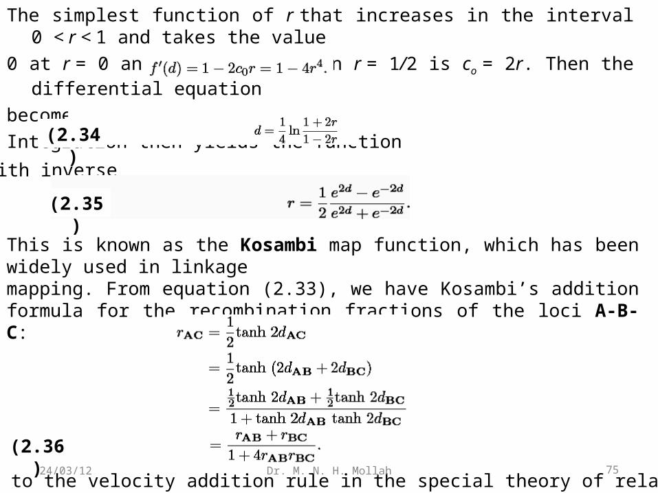
The simplest function of r that increases in the interval 0 < r < 1 and takes the value
0 at r = 0 and the value 1 when r = 1/2 is co = 2r. Then the differential equation
becomes
Integration then yields the function
with inverse
This is known as the Kosambi map function, which has been widely used in linkagemapping. From equation (2.33), we have Kosambi’s addition formula for the recombination fractions of the loci A-B-C:
This is similar to the velocity addition rule in the special theory of relativity.
(2.36)
(2.34)
(2.35)
75Dr. M. N. H. Mollah24/03/12
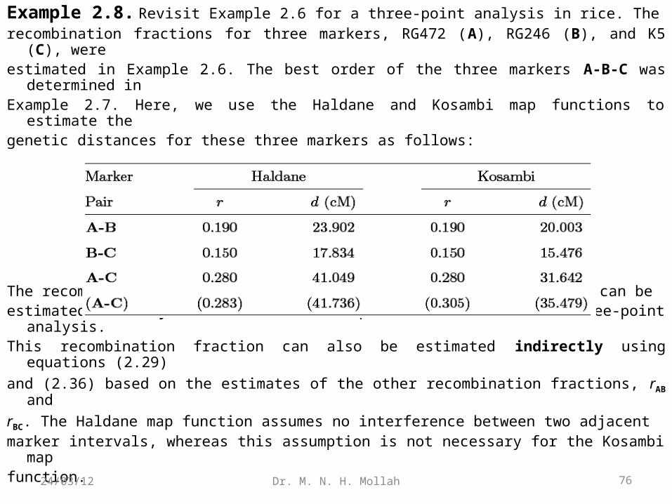
Example 2.8. Revisit Example 2.6 for a three-point analysis in rice. Therecombination fractions for three markers, RG472 (A), RG246 (B), and K5 (C), were estimated in Example 2.6. The best order of the three markers A-B-C was determined
in Example 2.7. Here, we use the Haldane and Kosambi map functions to estimate the genetic distances for these three markers as follows:
The recombination fraction between markers A and C at the two ends can beestimated directly on the basis of the procedure described in three-point analysis.This recombination fraction can also be estimated indirectly using equations (2.29)
and (2.36) based on the estimates of the other recombination fractions, rAB and
rBC. The Haldane map function assumes no interference between two adjacentmarker intervals, whereas this assumption is not necessary for the Kosambi map function. 76Dr. M. N. H. Mollah24/03/12
3.1 Introduction
3.2 Fully Informative Markers: A Diplotype Model 3.2.1 Two-Point Analysis 3.2.2 A More General Formulation 3.2.3 Three-Point Analysis 3.2.4 A More General Formulation
(3) A General Model for Linkage Analysis in Controlled Crosses
77Dr. M. N. H. Mollah24/03/12
3.1 IntroductionStatistical methods for linkage analysis in a backcross or F2 population derived fromtwo inbred lines were described in the previous slide. An advantage of linkageanalysis using these inbred line crosses is that the parental linkage phase betweendifferent genetic loci is known and therefore the patterns of marker segregation canbe determined and the linkage measured in terms of the recombination fraction tested.However, this inbred line-based analysis is not appropriate for outcrossing species inwhich it is not possible to generate homozygous lines through successive inbreeding.
A traditional strategy for estimating linkage phases is to account for all the possiblelinkage phases for given marker pairs and choose the most likely one based on theminimum recombination fraction and maximum likelihood value.
However, this strategy is not always statistically effective because the minimum estimate of the recombination fraction may be obtained from an incorrect linkage
phase.In this slide, a general framework for the simultaneous estimation of the linkage andlinkage phases is presented that can be viewed as a generalization of linkage analysis ininbred line crosses. 78Dr. M. N. H. Mollah24/03/12
3.2 Fully Informative Markers: A Diplotype Model
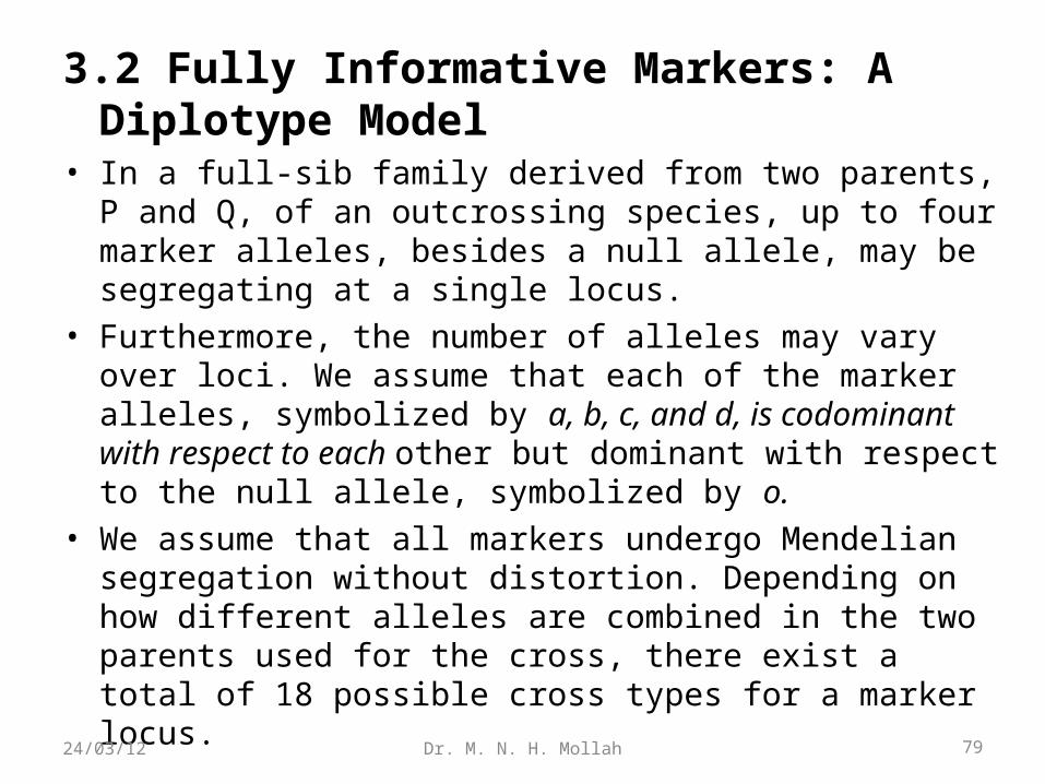
• In a full-sib family derived from two parents, P and Q, of an outcrossing species, up to four marker alleles, besides a null allele, may be segregating at a single locus.
• Furthermore, the number of alleles may vary over loci. We assume that each of the marker alleles, symbolized by a, b, c, and d, is codominant with respect to each other but dominant with respect to the null allele, symbolized by o.
• We assume that all markers undergo Mendelian segregation without distortion. Depending on how different alleles are combined in the two parents used for the cross, there exist a total of 18 possible cross types for a marker locus.
79Dr. M. N. H. Mollah24/03/12
3.2.1 Two-Point Analysis:
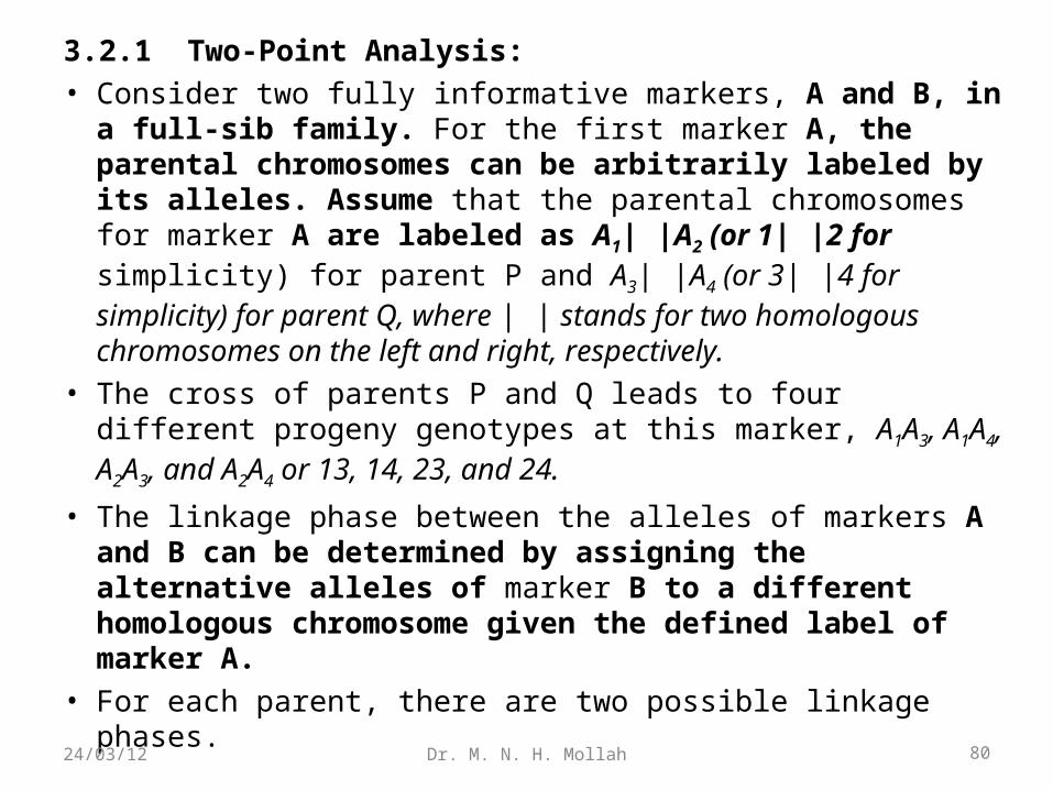
• Consider two fully informative markers, A and B, in a full-sib family. For the first marker A, the parental chromosomes can be arbitrarily labeled by its alleles. Assume that the parental chromosomes for marker A are labeled as A1| |A2 (or 1| |2 for simplicity) for parent P and A3| |A4 (or 3| |4 for simplicity) for parent Q, where | | stands for two homologous chromosomes on the left and right, respectively.
• The cross of parents P and Q leads to four different progeny genotypes at this marker, A1A3, A1A4, A2A3, and A2A4 or 13, 14, 23, and 24.
• The linkage phase between the alleles of markers A and B can be determined by assigning the alternative alleles of marker B to a different homologous chromosome given the defined label of marker A.
• For each parent, there are two possible linkage phases. 80Dr. M. N. H. Mollah24/03/12
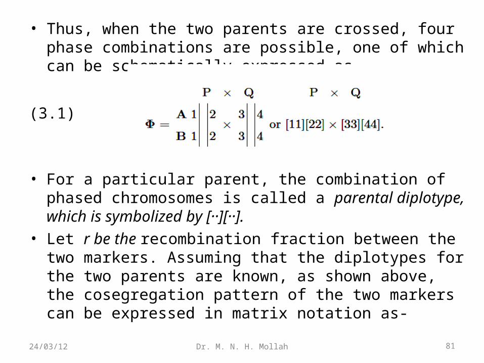
• Thus, when the two parents are crossed, four phase combinations are possible, one of which can be schematically expressed as
(3.1)
• For a particular parent, the combination of phased chromosomes is called a parental diplotype, which is symbolized by [··][··].
• Let r be the recombination fraction between the two markers. Assuming that the diplotypes for the two parents are known, as shown above, the cosegregation pattern of the two markers can be expressed in matrix notation as-
81Dr. M. N. H. Mollah24/03/12
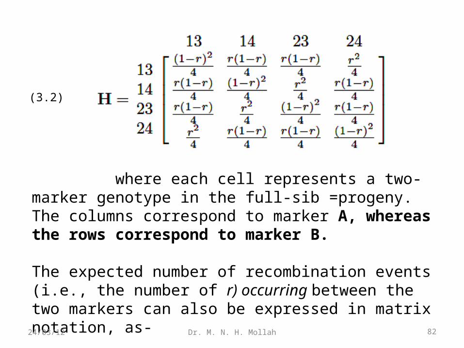
where each cell represents a two-marker genotype in the full-sib =progeny. The columns correspond to marker A, whereas the rows correspond to marker B.
The expected number of recombination events (i.e., the number of r) occurring between the two markers can also be expressed in matrix notation, as-
(3.2)
82Dr. M. N. H. Mollah24/03/12
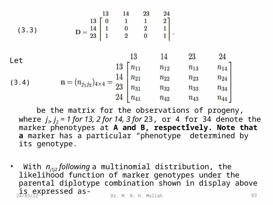
Let
be the matrix for the observations of progeny, where j1, j2 = 1 for 13, 2 for 14, 3 for 23, or 4 for 34 denote the marker phenotypes at A and B, respectively. Note that a marker has a particular “phenotype” determined by its genotype.
• With nj1j2 following a multinomial distribution, the likelihood function of marker genotypes under the parental diplotype combination shown in display above is expressed as-
(3.3)
(3.4)
83Dr. M. N. H. Mollah24/03/12
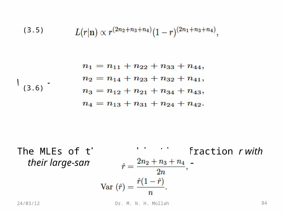
•
Where-
The MLEs of the recombination fraction r with their large-sample variances are thus-
(3.5)
(3.6)
84Dr. M. N. H. Mollah24/03/12
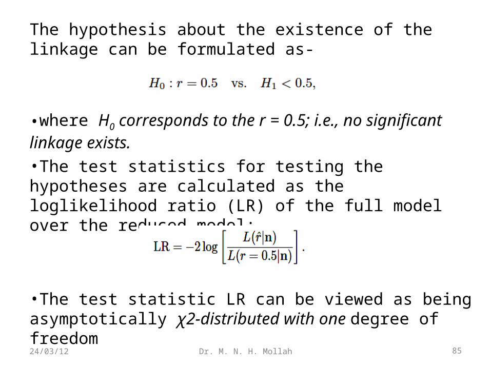
The hypothesis about the existence of the linkage can be formulated as-
•where H0 corresponds to the r = 0.5; i.e., no significant linkage exists.
•The test statistics for testing the hypotheses are calculated as the loglikelihood ratio (LR) of the full model over the reduced model:
•The test statistic LR can be viewed as being asymptotically χ2-distributed with one degree of freedom
85Dr. M. N. H. Mollah24/03/12
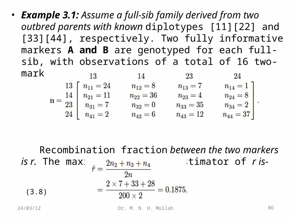
• Example 3.1: Assume a full-sib family derived from two outbred parents with known diplotypes [11][22] and [33][44], respectively. Two fully informative markers A and B are genotyped for each full-sib, with observations of a total of 16 two-marker genotypes as follows:
Recombination fraction between the two markers is r. The maximum likelihood estimator of r is-
(3.8)
86Dr. M. N. H. Mollah24/03/12
Where, n2 = 1+4+0+2 = 7, n3 = 8+11+2+12 = 33, and n4 = 7+7+8+6 = 28.
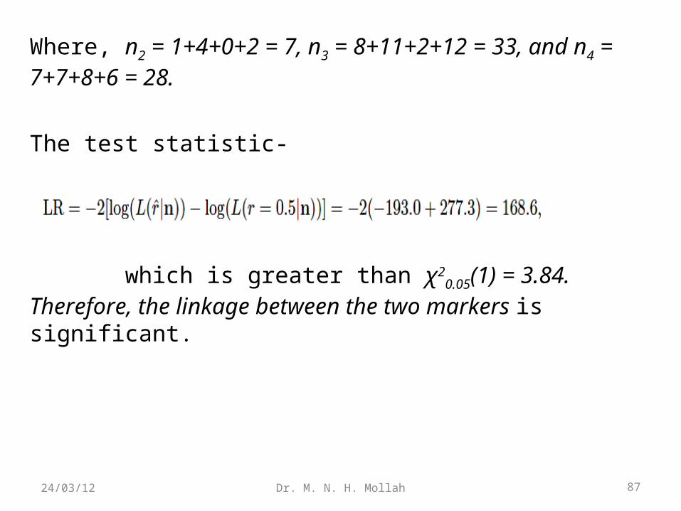
The test statistic-
which is greater than χ20.05(1) = 3.84. Therefore, the linkage
between the two markers is significant.
87Dr. M. N. H. Mollah24/03/12
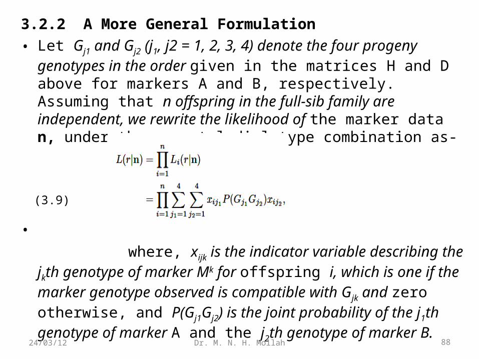
3.2.2 A More General Formulation
• Let Gj1 and Gj2 (j1, j2 = 1, 2, 3, 4) denote the four progeny genotypes in the order given in the matrices H and D above for markers A and B, respectively. Assuming that n offspring in the full-sib family are independent, we rewrite the likelihood of the marker data n, under the parental diplotype combination as-
•
where, xijk is the indicator variable describing the jkth genotype of marker Mk for offspring i, which is one if the marker genotype observed is compatible with Gjk and zero otherwise, and P(Gj1Gj2) is the joint probability of the j1th genotype of marker A and the j2th genotype of marker B.
(3.9)
88Dr. M. N. H. Mollah24/03/12
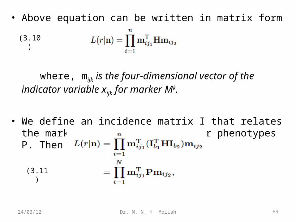
• Above equation can be written in matrix form as-
where, mijk is the four-dimensional vector of the indicator variable xijk for marker Mk.
• We define an incidence matrix I that relates the marker genotypes H to marker phenotypes P. Then we have,
(3.10)
(3.11)
89Dr. M. N. H. Mollah24/03/12
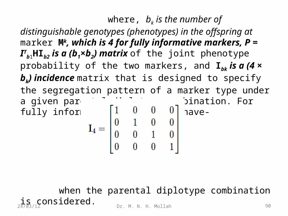
where, bk is the number of distinguishable genotypes (phenotypes) in the offspring at marker Mk, which is 4 for fully informative markers, P = IT
b1HIb2 is a (b1×b2) matrix of the joint phenotype probability of the two markers, and Ibk is a (4 × bk) incidence matrix that is designed to specify the segregation pattern of a marker type under a given parental diplotype combination. For fully informative markers, we have-
when the parental diplotype combination is considered.
90Dr. M. N. H. Mollah24/03/12
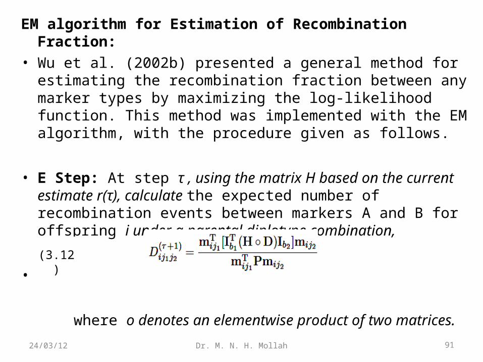
EM algorithm for Estimation of Recombination Fraction:
• Wu et al. (2002b) presented a general method for estimating the recombination fraction between any marker types by maximizing the log-likelihood function. This method was implemented with the EM algorithm, with the procedure given as follows.
• E Step: At step τ , using the matrix H based on the current estimate r(τ), calculate the expected number of recombination events between markers A and B for offspring i under a parental diplotype combination,
•
where o denotes an elementwise product of two matrices.
(3.12)
91Dr. M. N. H. Mollah24/03/12
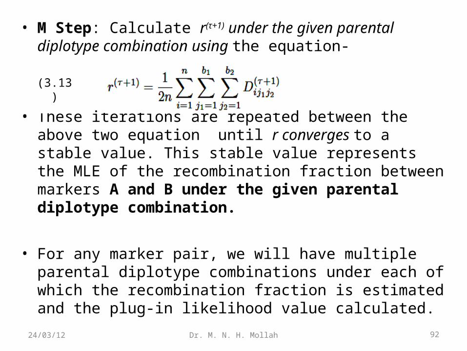
• M Step: Calculate r(τ+1) under the given parental diplotype combination using the equation-
• These iterations are repeated between the above two equation until r converges to a stable value. This stable value represents the MLE of the recombination fraction between markers A and B under the given parental diplotype combination.
• For any marker pair, we will have multiple parental diplotype combinations under each of which the recombination fraction is estimated and the plug-in likelihood value calculated.
(3.13)
92Dr. M. N. H. Mollah24/03/12
3.2.3 Three-Point Analysis
• Statistical algorithms for estimating the recombination fraction based on two-point analysis may not be powerful, especially in the case where partially informative markers are involved. Ridout et al. (1998) demonstrated an example in which three-point analysis can detect more linkage relationships between three loci than two-point analysis.
• Consider three markers in the order A-B-C. Relative to marker A, marker B has two possibilities to assign its alleles to two homologous chromosomes. Similarly, there are also two such allelic configurations for marker C when marker B is fixed. Thus, for one parent, there are 2 × 2 = 4 possible diplotypes. We assume that the diplotypes of two parents, P and Q, are known, as shown below:
93Dr. M. N. H. Mollah24/03/12
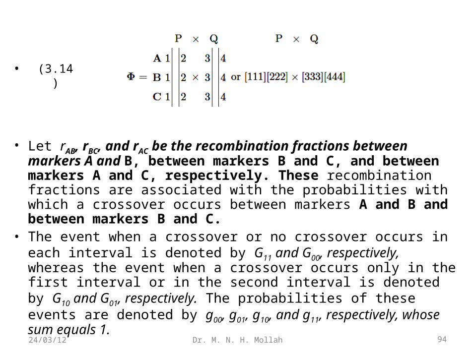
•
• Let rAB, rBC, and rAC be the recombination fractions between markers A and B, between markers B and C, and between markers A and C, respectively. These recombination fractions are associated with the probabilities with which a crossover occurs between markers A and B and between markers B and C.
• The event when a crossover or no crossover occurs in each interval is denoted by G11 and G00, respectively, whereas the event when a crossover occurs only in the first interval or in the second interval is denoted by G10 and G01, respectively. The probabilities of these events are denoted by g00, g01, g10, and g11, respectively, whose sum equals 1.
(3.14)
94Dr. M. N. H. Mollah24/03/12
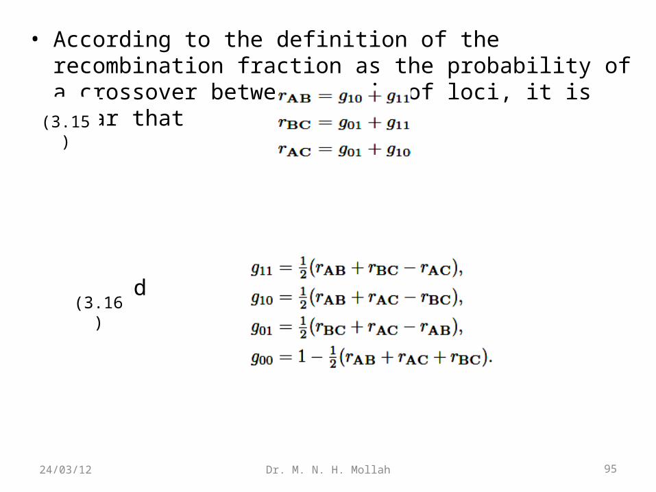
• According to the definition of the recombination fraction as the probability of a crossover between a pair of loci, it is clear that
and
(3.15)
(3.16)
95Dr. M. N. H. Mollah24/03/12
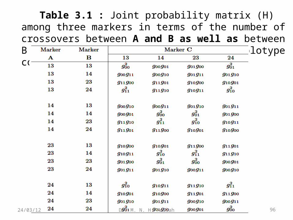
Table 3.1 : Joint probability matrix (H) among three markers in terms of the number of crossovers between A and B as well as between B and C under a particular parental diplotype combination.
96Dr. M. N. H. Mollah24/03/12
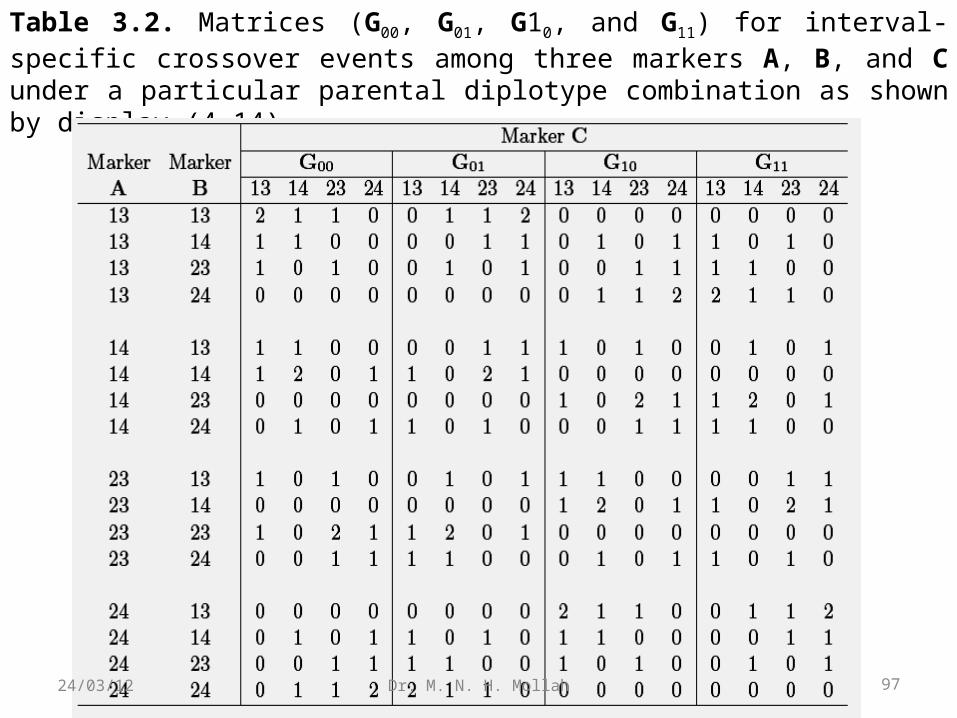
Table 3.2. Matrices (G00, G01, G10, and G11) for interval-specific crossover events among three markers A, B, and C under a particular parental diplotype combination as shown by display (4.14).
97Dr. M. N. H. Mollah24/03/12
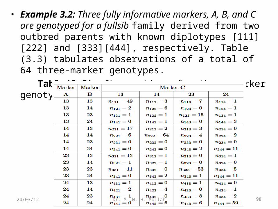
• Example 3.2: Three fully informative markers, A, B, and C are genotyped for a fullsib family derived from two outbred parents with known diplotypes [111][222] and [333][444], respectively. Table (3.3) tabulates observations of a total of 64 three-marker genotypes.
Table(3.3): Observations for three-marker genotypes in a full-sib family.
98Dr. M. N. H. Mollah24/03/12
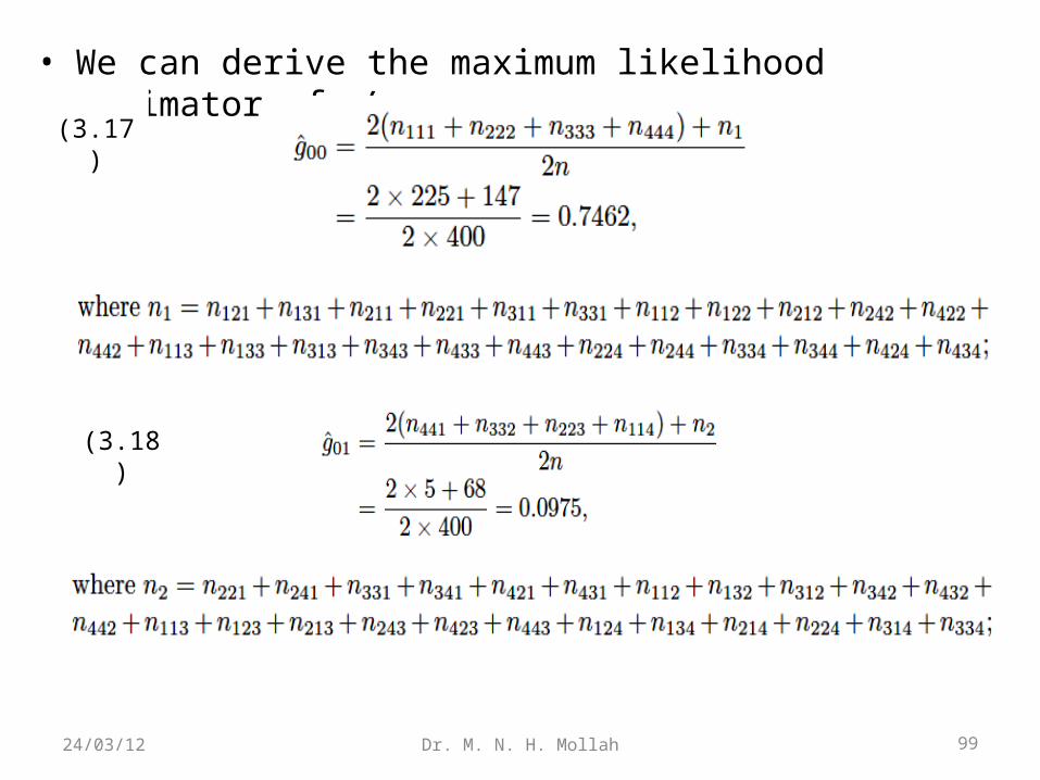
• We can derive the maximum likelihood estimator of g’s as
(3.17)
(3.18)
99Dr. M. N. H. Mollah24/03/12
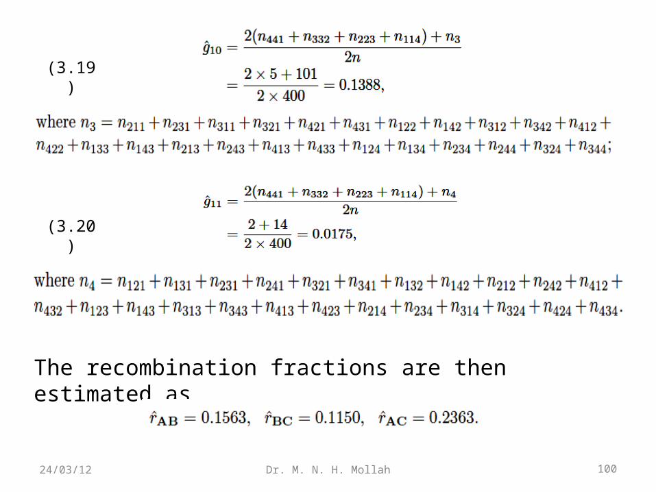
The recombination fractions are then estimated as
(3.19)
(3.20)
100Dr. M. N. H. Mollah24/03/12
4.1 Introduction
4.2 QTL Regression Model
4.3 Analysis at the Marker 4.3.1 Two-Sample t Test 4.3.2 Analysis of Variance 4.3.3 Genetic Analysis
4.4 Moving Away from the Marker 4.4.1 Likelihood
(4) QTL Analysis 1
101Dr. M. N. H. Mollah24/03/12
4.1 Introduction
The genome wide identification of QTLs, their locations and effects, is offundamental importance for agricultural, evolutionary, and biomedical genetics.
A variety of methods have been developed for QTL mapping (Hoeschele et al. 1997;
Lynch and Walsh 1998). These methods can be classified as t–tests and analysis ofvariance, least–squares analysis (LS), maximum likelihood analysis (ML), andBayesian analysis.
These methods differ in computational requirements, efficiency in terms ofextracting information, flexibility with regard to handling different data structures,and ability to map multiple QTLs. The simple LS method is efficient in terms ofcomputational speed but cannot extract all information from the data and is
restrictedto specific mating designs. The technique of ML interval mapping (Lander andBotstein 1989) is one of the most widely used methods for QTL analysis incontrolled crosses or structured pedigrees. The interval mapping method has beenextended to composite interval mapping (Zeng 1994) and multiple interval mapping(Kao et al. 1999). 102Dr. M. N. H. Mollah24/03/12
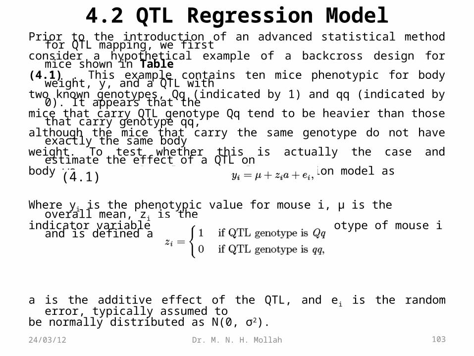
4.2 QTL Regression ModelPrior to the introduction of an advanced statistical method for QTL mapping, we
firstconsider a hypothetical example of a backcross design for mice shown in Table(4.1) . This example contains ten mice phenotypic for body weight, y, and a QTL
withtwo known genotypes, Qq (indicated by 1) and qq (indicated by 0). It appears that
themice that carry QTL genotype Qq tend to be heavier than those that carry genotype
qq,although the mice that carry the same genotype do not have exactly the same bodyweight. To test whether this is actually the case and estimate the effect of a QTL
onbody weight, we formulate a simple regression model as
Where yi is the phenotypic value for mouse i, μ is the overall mean, zi is theindicator variable that specifies the QTL genotype of mouse i and is defined as
a is the additive effect of the QTL, and ei is the random error, typically assumed tobe normally distributed as N(0, σ2).
(4.1)
103Dr. M. N. H. Mollah24/03/12
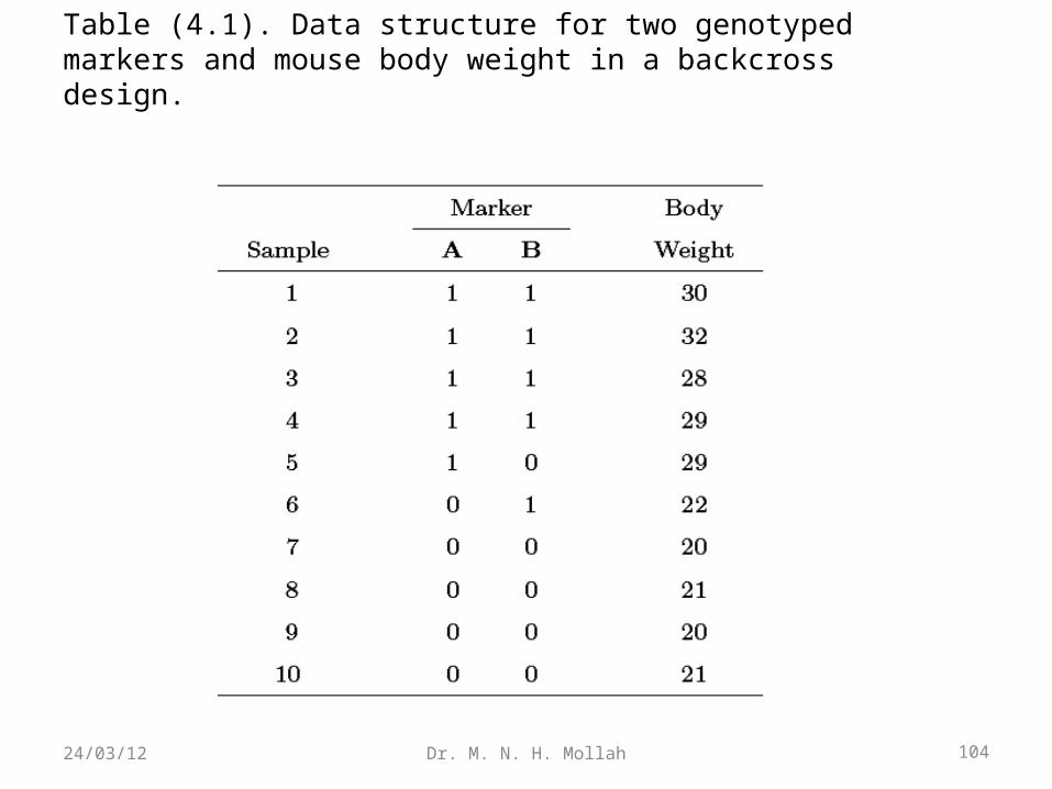
Table (4.1). Data structure for two genotyped markers and mouse body weight in a backcross design.
104Dr. M. N. H. Mollah24/03/12
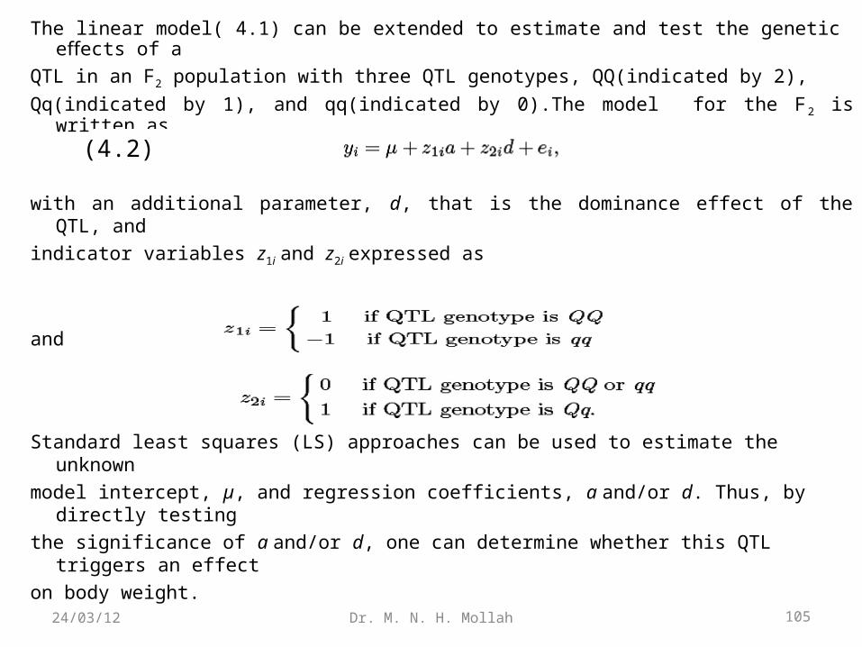
The linear model( 4.1) can be extended to estimate and test the genetic e ects of affQTL in an F2 population with three QTL genotypes, QQ(indicated by 2),
Qq(indicated by 1), and qq(indicated by 0).The model for the F2 is written as
with an additional parameter, d, that is the dominance effect of the QTL, and
indicator variables z1i and z2i expressed as
and
Standard least squares (LS) approaches can be used to estimate the unknown
model intercept, µ, and regression coefficients, a and/or d. Thus, by directly testing
the significance of a and/or d, one can determine whether this QTL triggers an effect
on body weight.
(4.2)
105Dr. M. N. H. Mollah24/03/12

Example 4.1. Assume a small population often backcrosses mice. Each mouse
was genotyped for two markers and measured for body weight as well. The marker
and phenotypic data are given in Table (4.1). With this table, we provide a procedure
for the estimation and test of the genetic e ect, a,of the QTL on mouse body weight.ffLet
106Dr. M. N. H. Mollah24/03/12
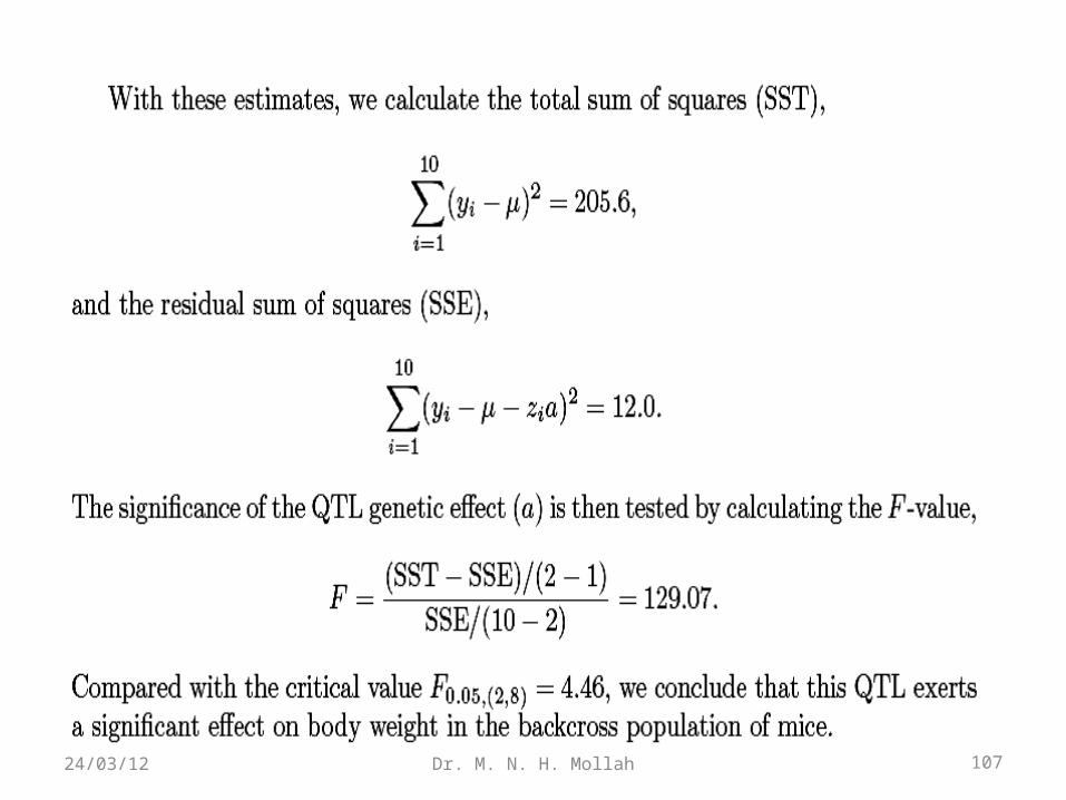
107Dr. M. N. H. Mollah24/03/12
4.3 Analysis at the MarkerA QTL statistical model assumes that the QTL genotypes can be observed in a
mapping population. This is not possible in practice. What we can do is to use
observable markers to predict such unobservable QTLs through the linkage between
markers and QTLs. Thus, by performing the association analysis between the markers
and phenotypes, we can still infer the effect of a putative QTL on phenotypic
variation.
The use of a single-marker is limited for QTL identification since it cannot determine
at which side of the marker, left or right, the QTL is located. However, single
marker analyses are useful for a preliminary test of the existence of a QTL, although
they cannot estimate the QTL location. Below, we introduce two testing approaches
for marker analysis based on the t and F test statistics.
108Dr. M. N. H. Mollah24/03/12
4.3.1 Two-Sample t TestThe mouse backcross data in Table (4.1) are genotyped for two linked molecular
markers A and B and are given in Table (4.1). Two genotypes at each marker are
denoted by 1 and 0. The linkage between these two markers can be seen from the
consistency of their genotypes among the samples, except for mice 5 and 6. The
recombination fraction between the two markers is r = 2/10 = 0.2.We will analyze
these two markers separately.
Let μ1 and μ0 be the true trait means of two different groups of mice with
genotypes 1 and 0, respectively, and let m1 and m0 be the corresponding sample
means. The hypotheses for the test can be formulated as
The t test statistic used to test for the significance of the difference between the two means is
(4.3)
109Dr. M. N. H. Mollah24/03/12
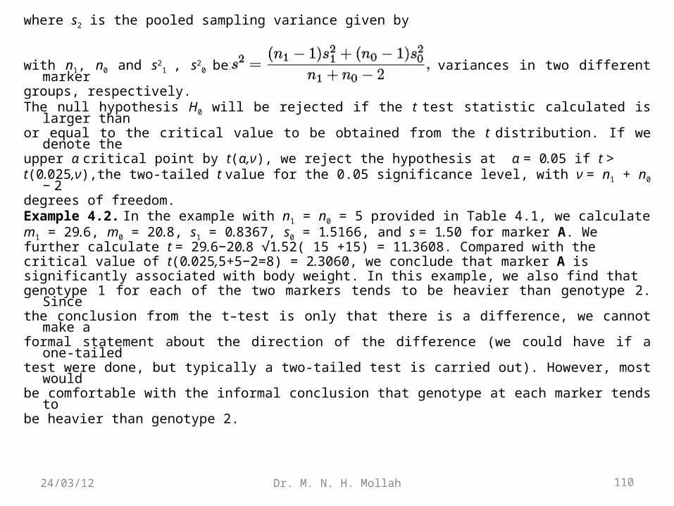
where s2 is the pooled sampling variance given by
with n1, n0 and s21 , s2
0 being the sample sizes and variances in two different markergroups, respectively. The null hypothesis H0 will be rejected if the t test statistic calculated is larger thanor equal to the critical value to be obtained from the t distribution. If we denote theupper α critical point by t(α,ν), we reject the hypothesis at α = 0.05 if t >t(0.025,ν),the two-tailed t value for the 0.05 significance level, with ν = n1 + n0 − 2degrees of freedom.Example 4.2. In the example with n1 = n0 = 5 provided in Table 4.1, we calculatem1 = 29.6, m0 = 20.8, s1 = 0.8367, s0 = 1.5166, and s = 1.50 for marker A. Wefurther calculate t = 29.6−20.8 √1.52( 15 +15) = 11.3608. Compared with thecritical value of t(0.025,5+5−2=8) = 2.3060, we conclude that marker A issignificantly associated with body weight. In this example, we also find thatgenotype 1 for each of the two markers tends to be heavier than genotype 2. Since the conclusion from the t–test is only that there is a difference, we cannot make aformal statement about the direction of the difference (we could have if a one-tailedtest were done, but typically a two-tailed test is carried out). However, most wouldbe comfortable with the informal conclusion that genotype at each marker tends tobe heavier than genotype 2.
110Dr. M. N. H. Mollah24/03/12
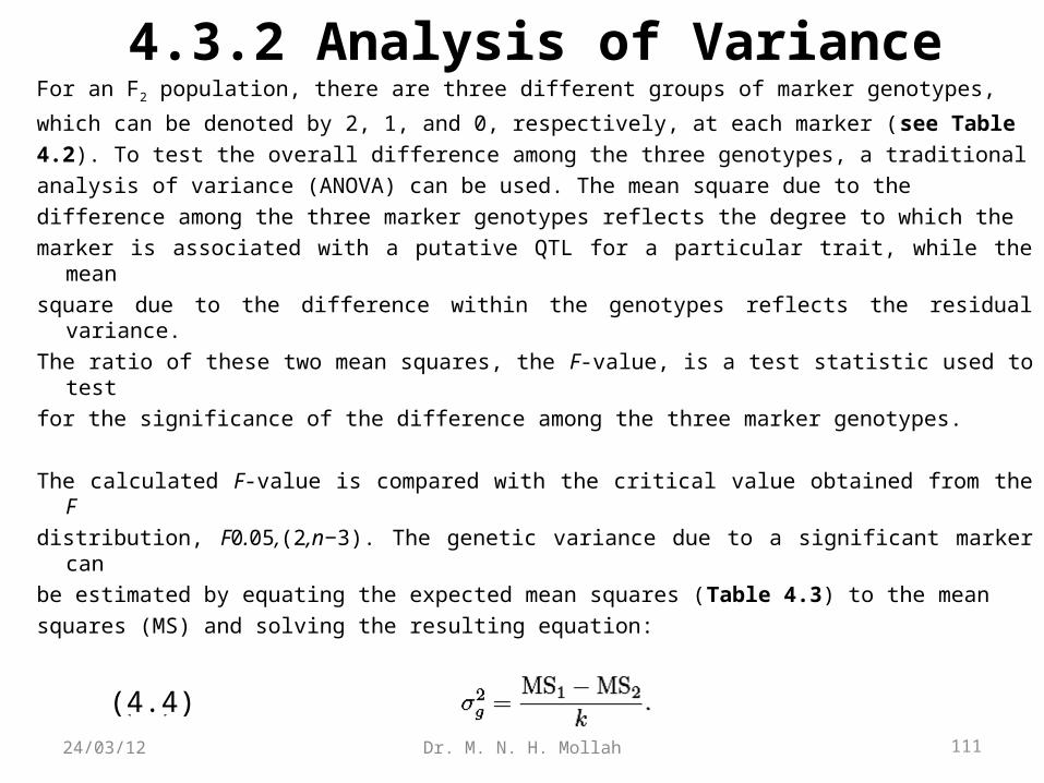
4.3.2 Analysis of VarianceFor an F2 population, there are three different groups of marker genotypes,
which can be denoted by 2, 1, and 0, respectively, at each marker (see Table
4.2). To test the overall difference among the three genotypes, a traditional
analysis of variance (ANOVA) can be used. The mean square due to the
difference among the three marker genotypes reflects the degree to which the
marker is associated with a putative QTL for a particular trait, while the mean
square due to the difference within the genotypes reflects the residual variance.
The ratio of these two mean squares, the F-value, is a test statistic used to test
for the significance of the difference among the three marker genotypes.
The calculated F-value is compared with the critical value obtained from the F
distribution, F0.05,(2,n−3). The genetic variance due to a significant marker can
be estimated by equating the expected mean squares (Table 4.3) to the mean
squares (MS) and solving the resulting equation:
(4.4)
111Dr. M. N. H. Mollah24/03/12
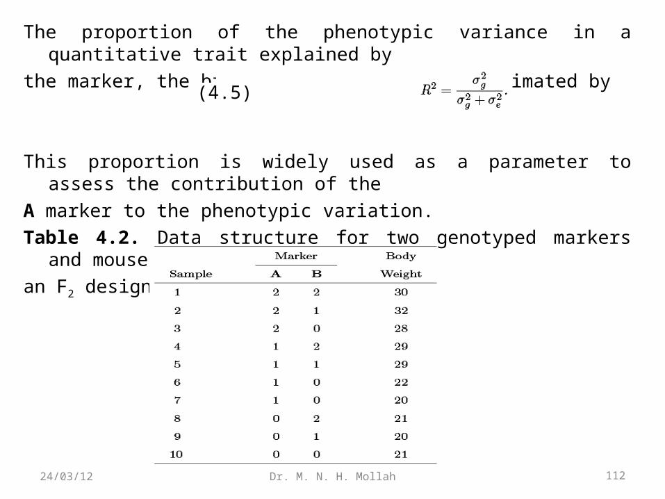
The proportion of the phenotypic variance in a quantitative trait explained by
the marker, the broad-sense heritability, is estimated by
This proportion is widely used as a parameter to assess the contribution of the
A marker to the phenotypic variation.
Table 4.2. Data structure for two genotyped markers and mouse body weight in
an F2 design.
(4.5)
112Dr. M. N. H. Mollah24/03/12
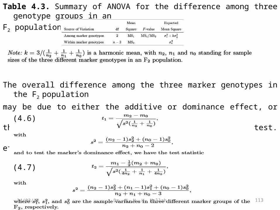
Table 4.3. Summary of ANOVA for the difference among three genotype groups in an
F2 population.
The overall difference among the three marker genotypes in the F2 population
may be due to either the additive or dominance effect, or both. The significance of
these two effects can also be tested by using the t test. To test the marker’s additive
effect, we have the test statistic(4.6)
(4.7)
113Dr. M. N. H. Mollah24/03/12
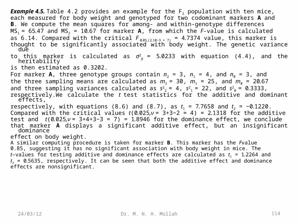
Example 4.5. Table 4.2 provides an example for the F2 population with ten mice,each measured for body weight and genotyped for two codominant markers A andB. We compute the mean squares for among- and within-genotype differences MS1 = 65.47 and MS2 = 10.67 for marker A, from which the F-value is calculatedas 6.14. Compared with the critical F 0.05,(2,10−3 = 7) = 4.7374 value, this marker isthought to be significantly associated with body weight. The genetic variance dueto this marker is calculated as σ2
g = 5.0233 with equation (4.4), and the heritabilityis then estimated as 0.3202.For marker A, three genotype groups contain n2 = 3, n1 = 4, and n0 = 3, andthe three sampling means are calculated as m2 = 30, m1 = 25, and m0 = 20.67and three sampling variances calculated as s2
2 = 4, s21 = 22, and s2
0 = 0.3333,respectively.We calculate the t test statistics for the additive and dominant effects,respectively, with equations (8.6) and (8.7), as t1 = 7.7658 and t2 = −0.1220.Compared with the critical values t(0.025,ν = 3+3−2 = 4) = 2.1318 for the additivetest and t(0.025,ν = 3+4+3−3 = 7) = 1.8946 for the dominance effect, we concludethat marker A displays a significant additive effect, but an insignificant dominanceeffect on body weight.A similar computing procedure is taken for marker B. This marker has the Fvalue0.85, suggesting it has no significant association with body weight in mice. Thet–values for testing additive and dominance effects are calculated as t1 = 1.2264 andt2 = 0.5635, respectively. It can be seen that both the additive effect and dominanceeffects are nonsignificant.
114Dr. M. N. H. Mollah24/03/12
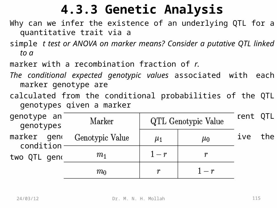
4.3.3 Genetic AnalysisWhy can we infer the existence of an underlying QTL for a quantitative trait via a
simple t test or ANOVA on marker means? Consider a putative QTL linked to a
marker with a recombination fraction of r.
The conditional expected genotypic values associated with each marker genotype are
calculated from the conditional probabilities of the QTL genotypes given a marker
genotype and from the genotypic values of different QTL genotypes. Given known
marker genotypes, Aa (1) and aa (0), we can derive the conditional probabilities of
two QTL genotypes, Qq (1) and qq(0), for the backcross as
115Dr. M. N. H. Mollah24/03/12
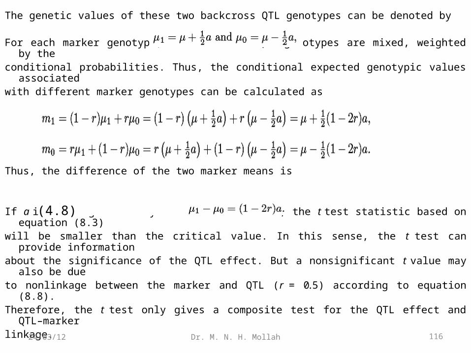
The genetic values of these two backcross QTL genotypes can be denoted by
For each marker genotype, two different QTL genotypes are mixed, weighted by theconditional probabilities. Thus, the conditional expected genotypic values associatedwith different marker genotypes can be calculated as
Thus, the difference of the two marker means is
If a is not significantly different from zero, the t test statistic based on equation (8.3)will be smaller than the critical value. In this sense, the t test can provide informationabout the significance of the QTL effect. But a nonsignificant t value may also be dueto nonlinkage between the marker and QTL (r = 0.5) according to equation (8.8).Therefore, the t test only gives a composite test for the QTL effect and QTL–markerlinkage.
(4.8)
116Dr. M. N. H. Mollah24/03/12
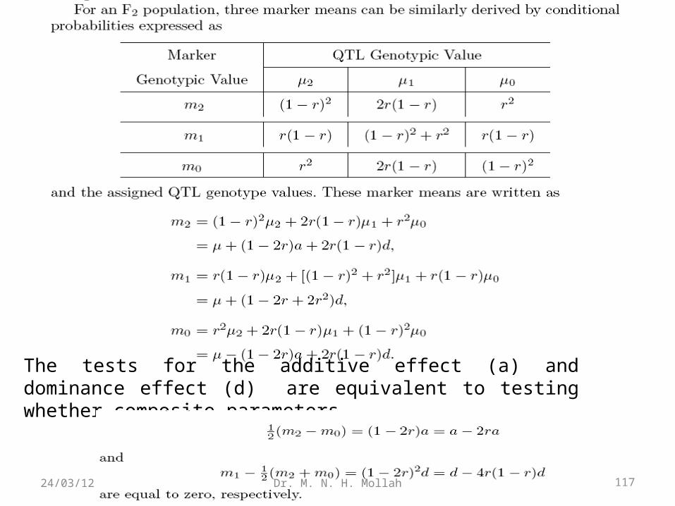
The tests for the additive effect (a) and dominance effect (d) are equivalent to testing whether composite parameters
117Dr. M. N. H. Mollah24/03/12
From the analysis above, although the t test and ANOVA can be usedto test the significance of marker differences, they cannot separate
QTLgenotypic means and the recombination fraction between a singlemarker and a QTL. If the marker difference is significant, as shown forthe two markers in mouse body weight, we still do not know whetherthis difference is due to a tight linkage (small r) between the markerand a QTL of small effect or a loose linkage (large r) between themarker and a QTL of large effect.
In fact, the additive and dominance effects of QTLs are underestimatedby 2r and 4r(1−r), respectively, from a simple comparison of markermeans. Also, the t test and ANOVA cannot separate the effects ofindividual QTLs on the phenotype if there are two or more QTL on thesame chromosome. The two confounded parameters, QTL geneticmeans and the recombination fraction, can be separated using theapproaches explained below.
118Dr. M. N. H. Mollah24/03/12
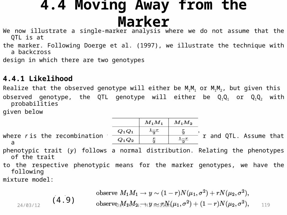
4.4 Moving Away from the MarkerWe now illustrate a single-marker analysis where we do not assume that the QTL is atthe marker. Following Doerge et al. (1997), we illustrate the technique with a
backcrossdesign in which there are two genotypes
4.4.1 LikelihoodRealize that the observed genotype will either be M1M1 or M1M2, but given this
observed genotype, the QTL genotype will either be Q1Q1 or Q1Q2 with probabilitiesgiven below
where r is the recombination fraction between the marker and QTL. Assume that aphenotypic trait (y) follows a normal distribution. Relating the phenotypes of the traitto the respective phenotypic means for the marker genotypes, we have the followingmixture model:
(4.9)119Dr. M. N. H. Mollah24/03/12
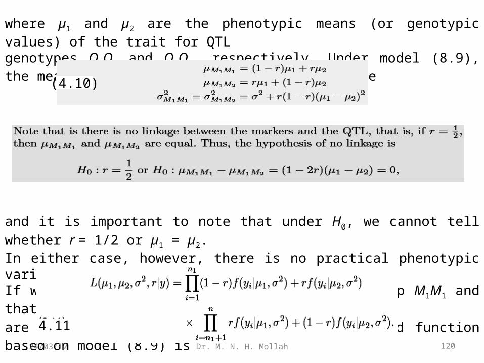
where µ1 and µ2 are the phenotypic means (or genotypic values) of the trait for QTLgenotypes Q1Q1 and Q1Q2, respectively. Under model (8.9), the mean and variance of the distributions are
and it is important to note that under H0, we cannot tell whether r = 1/2 or µ1 = µ2.In either case, however, there is no practical phenotypic variation detectable.If we assume that y1, . . . , yn1 are from marker group M1M1 and that yn1+1, . . . , yn
are from marker group M1M2, then the likelihood function based on model (8.9) is
(4.10)
4.11
120Dr. M. N. H. Mollah24/03/12
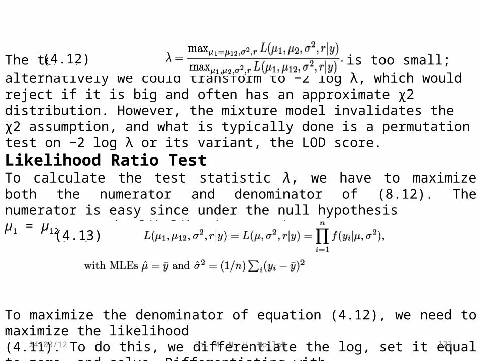
To test the null hypothesis of no linkage, H0 : no QTL, we could use the likelihood ratio statistic
The test statistic λ would reject H0 if it is too small; alternatively we could transform to −2 log λ, which would reject if it is big and often has an approximate χ2 distribution. However, the mixture model invalidates the χ2 assumption, and what is typically done is a permutation test on −2 log λ or its variant, the LOD score.
Likelihood Ratio TestTo calculate the test statistic λ, we have to maximize both the numerator and denominator of (8.12). The numerator is easy since under the null hypothesis µ1 = µ12 = µ, the likelihood (4.11) becomes
To maximize the denominator of equation (4.12), we need to maximize the likelihood(4.11). To do this, we differentiate the log, set it equal to zero, and solve. Differentiating withrespect to µ1 gives
(4.12)
(4.13)
121Dr. M. N. H. Mollah24/03/12
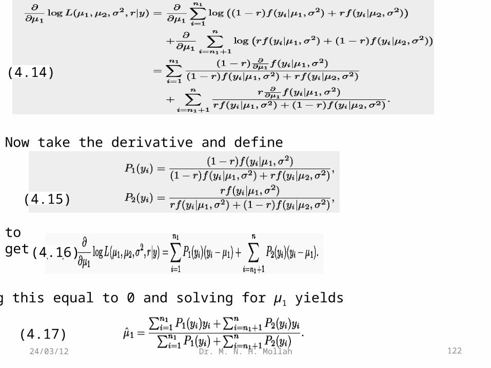
Now take the derivative and define
to get
Setting this equal to 0 and solving for µ1 yields
(4.14)
(4.15)
(4.16)
(4.17)122Dr. M. N. H. Mollah24/03/12
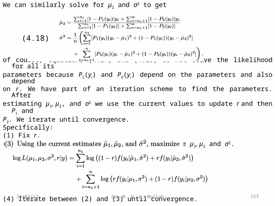
We can similarly solve for µ2 and σ2 to get
of course, equations (4.17) and (4.18) do not solve the likelihood for all itsparameters because P1(yi) and P2(yi) depend on the parameters and also dependon r. We have part of an iteration scheme to find the parameters. Afterestimating µ1, µ2, and σ2 we use the current values to update r and then P1 andP2. We iterate until convergence.Specifically:(1) Fix r.(2) Use equations (4.17) and (4.18) to estimate µ1, µ2 and σ2.
(4) Iterate between (2) and (3) until convergence.
(4.18)
123Dr. M. N. H. Mollah24/03/12
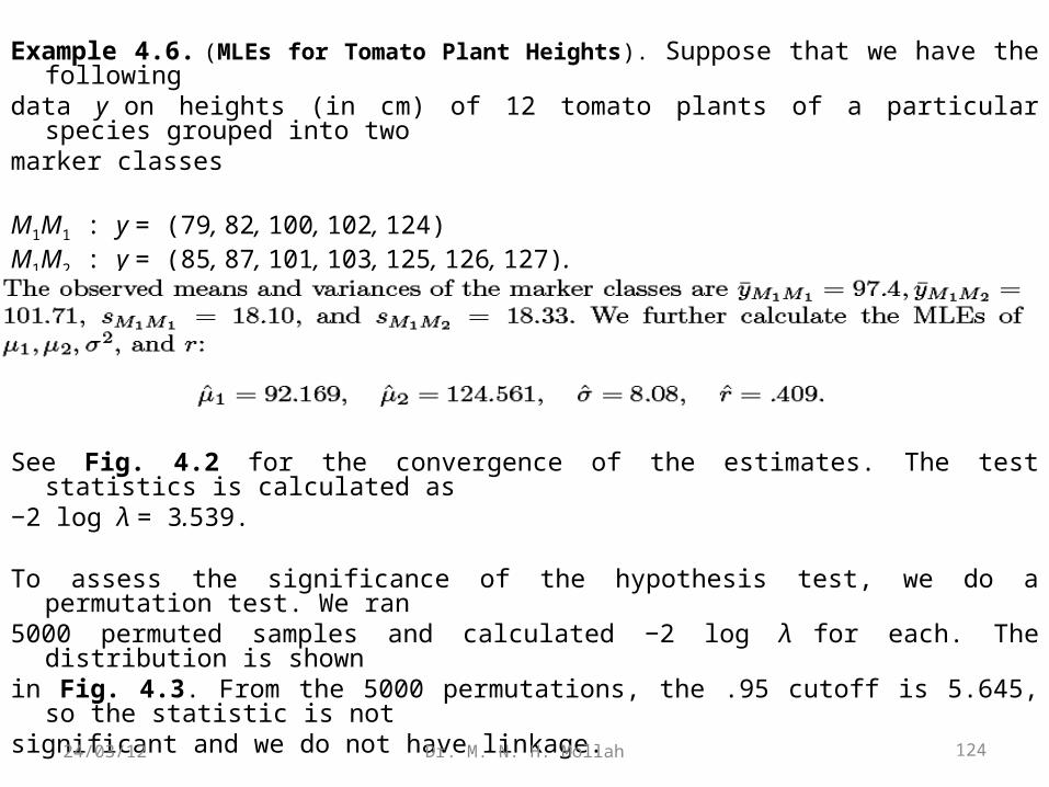
Example 4.6. (MLEs for Tomato Plant Heights). Suppose that we have the followingdata y on heights (in cm) of 12 tomato plants of a particular species grouped into twomarker classes
M1M1 : y = (79, 82, 100, 102, 124)M1M2 : y = (85, 87, 101, 103, 125, 126, 127).
See Fig. 4.2 for the convergence of the estimates. The test statistics is calculated as −2 log λ = 3.539.
To assess the significance of the hypothesis test, we do a permutation test. We ran5000 permuted samples and calculated −2 log λ for each. The distribution is shownin Fig. 4.3. From the 5000 permutations, the .95 cutoff is 5.645, so the statistic is notsignificant and we do not have linkage.
124Dr. M. N. H. Mollah24/03/12
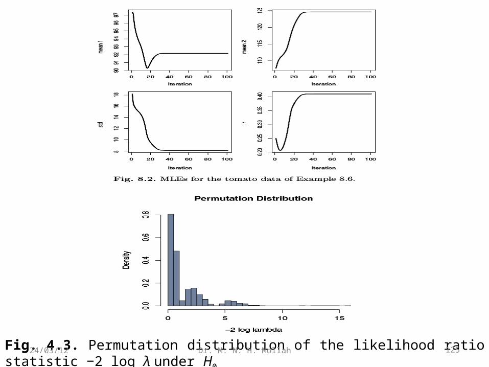
Fig. 4.3. Permutation distribution of the likelihood ratio statistic −2 log λ under H0
based on 5000 permutations.125Dr. M. N. H. Mollah24/03/12
5.1 Introduction
5.2 Linear Regression Model
5.3 Interval Mapping in the Backcross
5.3.1 Conditional Probabilities
5.3.2 Conditional Regression Model
5.3.3 Estimation and Test
5.4 Interval Mapping in an F2
(5) QTL Analysis 2
126Dr. M. N. H. Mollah24/03/12
5.1 IntroductionThe genetic analysis of quantitative traits includes two major tasks: (1)identifying the location of QTLs affecting a quantitative trait using a geneticlinkage map constructed from molecular markers, and (2) estimating thegenetic effects of the QTLs on the phenotype. If the genotypes of a putativeQTL were known for all individuals, its genomic location could be readilydetermined using a marker linkage analysis. Furthermore, the genetic effects ofthe QTL could be precisely estimated and tested by simple t tests or ANOVA.However, it is not possible for the genotypes of QTLs to be directly observed;instead they should be inferred from observed marker and phenotypicinformation. To rule out the genetic effect and position of a QTL, a moreadvanced statistical analysis should be adopted. The central idea ofindividually estimating the QTL effect and position is to formulate a statisticalmodel for observed marker and phenotypic data in terms of the underlyingQTL that is located between two flanking markers. This so-called intervalmapping approach can overcome the confounding problem of the marker–QTLrecombination fraction and QTL effects through the conditionalprobabilities of unknown QTL genotypes given observed marker genotypes.
127Dr. M. N. H. Mollah24/03/12
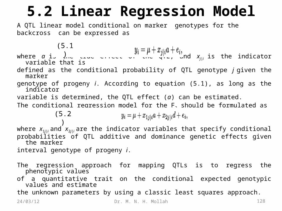
5.2 Linear Regression ModelA QTL linear model conditional on marker genotypes for thebackcross can be expressed as
where a is the true effect of the QTL, and xj|i is the indicator variable that isdefined as the conditional probability of QTL genotype j given the markergenotype of progeny i. According to equation (5.1), as long as the indicatorvariable is determined, the QTL effect (a) can be estimated.The conditional regression model for the F2 should be formulated as
where x1j|i and x2j|i are the indicator variables that specify conditionalprobabilities of QTL additive and dominance genetic effects given the markerinterval genotype of progeny i.
The regression approach for mapping QTLs is to regress the phenotypic valuesof a quantitative trait on the conditional expected genotypic values and estimatethe unknown parameters by using a classic least squares approach.
(5.1)
(5.2)
128Dr. M. N. H. Mollah24/03/12
5.3 Interval Mapping in the Backcross5.3.1 Conditional Probabilities
Table 5.1 integrates information from the QTL table and marker table. Supposethere is a putative QTL that is bracketed by two linked markers M and N. For anobservable marker genotype, there are two possibilities to carry a QTL genotype,Qq (1) or qq (0). Table 5.1 also provides possible marker-QTL-markergenotypes. Let ω1|i and ω0|i be the conditional probabilities of two QTL genotypesgiven a two-marker genotype for mouse i.
The values of ω1|i and ω0|i depend on the recombination fractions between thetwo markers (r), between marker M and QTL (r1), and between QTL and markerN (r2). A triply heterozygous F1 backcrossed to a parent will generate eightthreepoint (marker-QTL-marker) genotypes: 111, 101, 110, 100, 011, 001, 010, and000. These genotype frequencies are derived under the assumption of no doublecrossover and are expressed in Table 10.2. Thus, the conditional probabilities of theQTL genotypes given the marker genotypes of the interval in the backcross can bederived according to Bayes’ theorem, and are expressed in Table 5.3.
129Dr. M. N. H. Mollah24/03/12
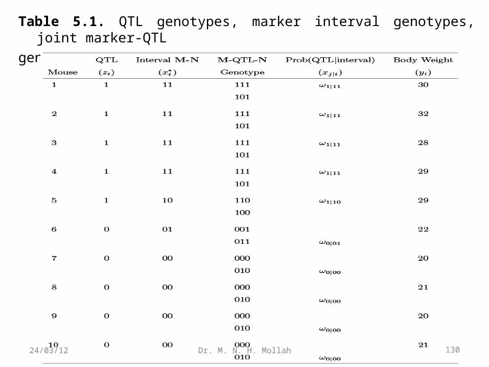
Table 5.1. QTL genotypes, marker interval genotypes, joint marker-QTL
genotypes and mouse body weight in a backcross design.
130Dr. M. N. H. Mollah24/03/12
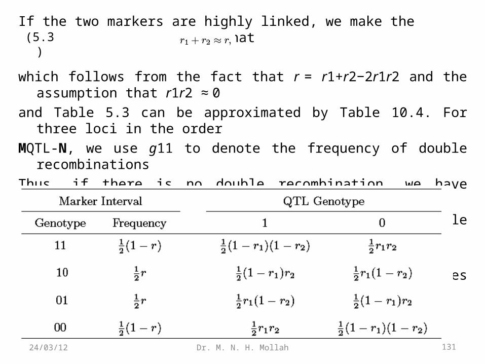
If the two markers are highly linked, we make the simplifying assumption that
which follows from the fact that r = r1+r2−2r1r2 and the assumption that r1r2 ≈ 0
and Table 5.3 can be approximated by Table 10.4. For three loci in the order
MQTL-N, we use g11 to denote the frequency of double recombinations
Thus, if there is no double recombination, we have equation (5.3). In other words,
for a highly dense map, we can assume that no double recombinations occur
between the adjacent intervals.
Table 5.2. Joint marker-QTL-marker genotype frequencies in the backcross.
(5.3)
131Dr. M. N. H. Mollah24/03/12
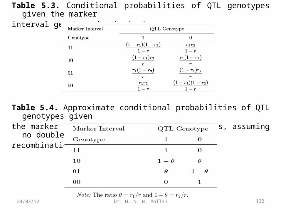
Table 5.3. Conditional probabilities of QTL genotypes given the markerinterval genotype in the backcross.
Table 5.4. Approximate conditional probabilities of QTL genotypes giventhe marker interval genotype in the backcross, assuming no doublerecombination.
132Dr. M. N. H. Mollah24/03/12
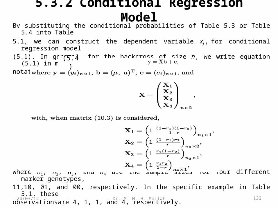
5.3.2 Conditional Regression ModelBy substituting the conditional probabilities of Table 5.3 or Table 5.4 into Table
5.1, we can construct the dependent variable xj|i for conditional regression model(5.1). In general, for the backcross of size n, we write equation (5.1) in matrixnotation as
where n1, n2, n3, and n4 are the sample sizes for four different marker genotypes,11,10, 01, and 00, respectively. In the specific example in Table 5.1, theseobservationsare 4, 1, 1, and 4, respectively.
(5.4)
133Dr. M. N. H. Mollah24/03/12
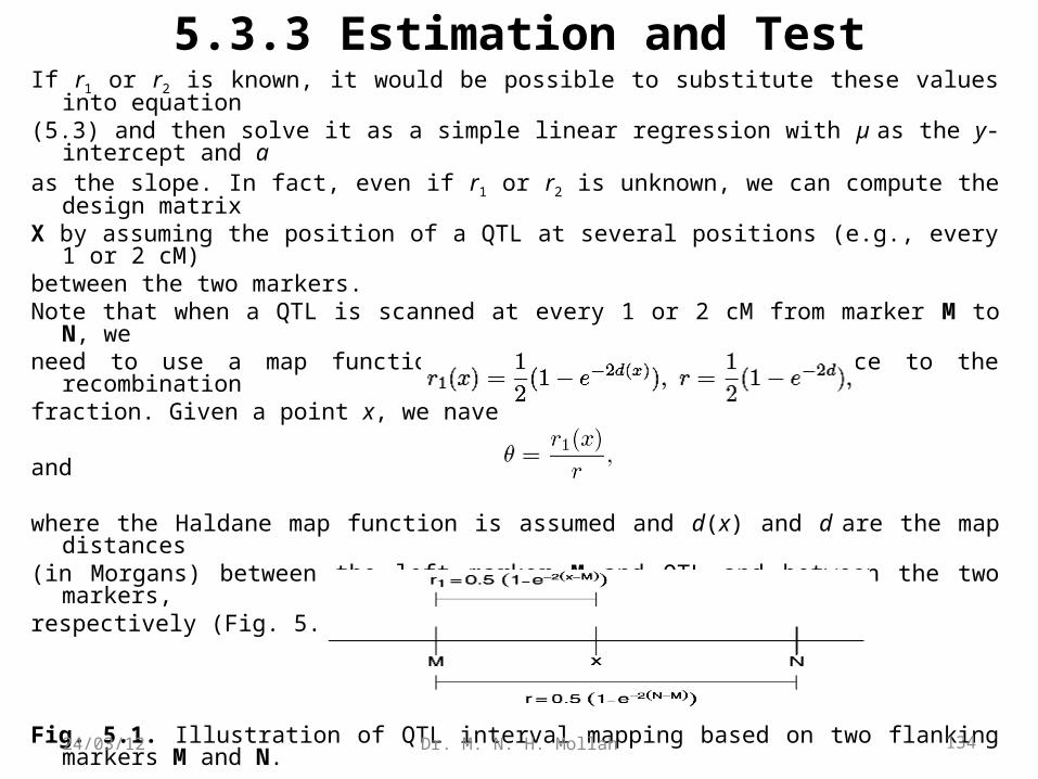
5.3.3 Estimation and TestIf r1 or r2 is known, it would be possible to substitute these values into equation(5.3) and then solve it as a simple linear regression with µ as the y-intercept and aas the slope. In fact, even if r1 or r2 is unknown, we can compute the design matrixX by assuming the position of a QTL at several positions (e.g., every 1 or 2 cM)between the two markers.Note that when a QTL is scanned at every 1 or 2 cM from marker M to N, weneed to use a map function to convert the map distance to the recombinationfraction. Given a point x, we have
and
where the Haldane map function is assumed and d(x) and d are the map distances(in Morgans) between the left marker M and QTL and between the two markers,respectively (Fig. 5.1).
Fig. 5.1. Illustration of QTL interval mapping based on two flanking markers M and N.
134Dr. M. N. H. Mollah24/03/12
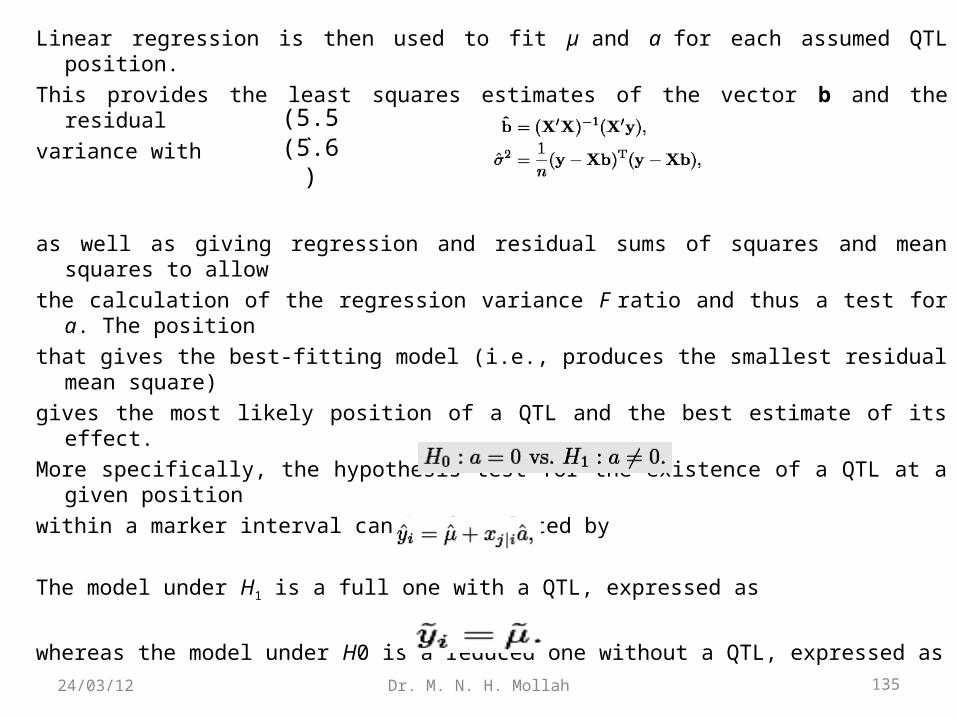
Linear regression is then used to fit µ and a for each assumed QTL position.
This provides the least squares estimates of the vector b and the residual
variance with
as well as giving regression and residual sums of squares and mean squares to allow
the calculation of the regression variance F ratio and thus a test for a. The position
that gives the best-fitting model (i.e., produces the smallest residual mean square)
gives the most likely position of a QTL and the best estimate of its effect.
More specifically, the hypothesis test for the existence of a QTL at a given position
within a marker interval can be formulated by
The model under H1 is a full one with a QTL, expressed as
whereas the model under H0 is a reduced one without a QTL, expressed as
(5.5)(5.6)
135Dr. M. N. H. Mollah24/03/12
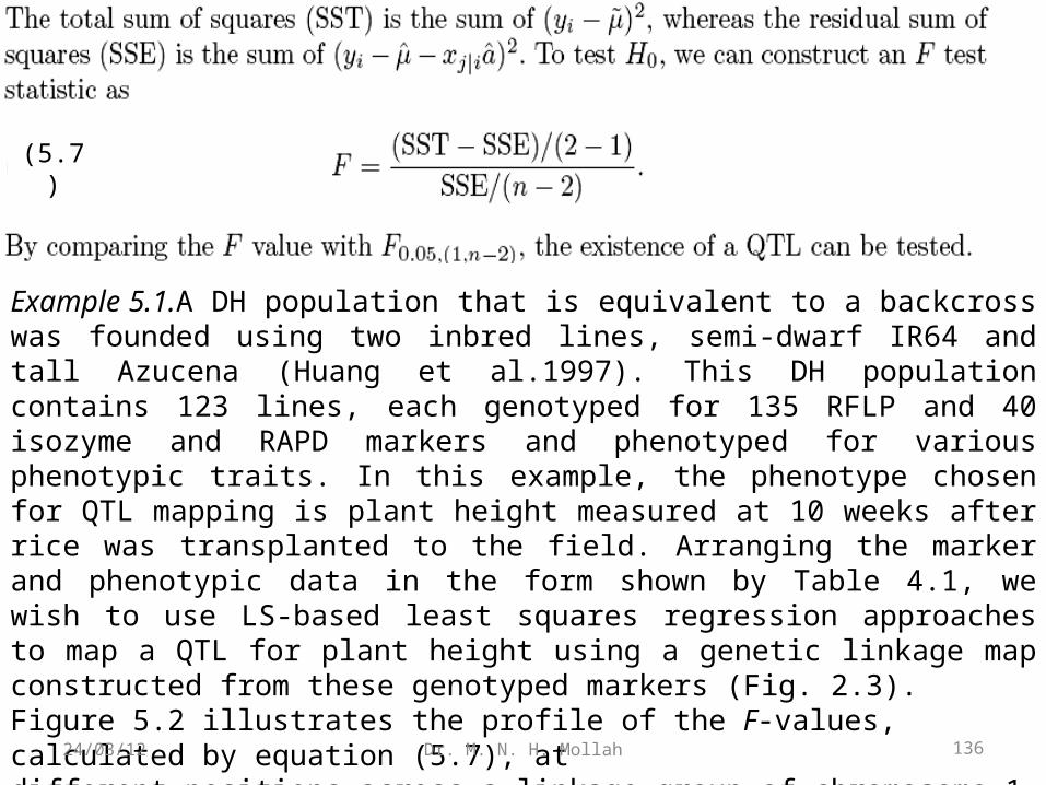
Example 5.1.A DH population that is equivalent to a backcross was founded using two inbred lines, semi-dwarf IR64 and tall Azucena (Huang et al.1997). This DH population contains 123 lines, each genotyped for 135 RFLP and 40 isozyme and RAPD markers and phenotyped for various phenotypic traits. In this example, the phenotype chosen for QTL mapping is plant height measured at 10 weeks after rice was transplanted to the field. Arranging the marker and phenotypic data in the form shown by Table 4.1, we wish to use LS-based least squares regression approaches to map a QTL for plant height using a genetic linkage map constructed from these genotyped markers (Fig. 2.3).Figure 5.2 illustrates the profile of the F-values, calculated by equation (5.7), atdifferent positions across a linkage group of chromosome 1 constructed by 18 markers.There is a clear peak at 199 cM in the marker interval [RZ730–RZ801], whose F-value,88.02, is largely beyond the critical F0.05,(1,85) = 3.95 (87 rice left due to missing datain these two markers). This suggests the existence of a significant QTL around thatposition.
(5.7)
136Dr. M. N. H. Mollah24/03/12
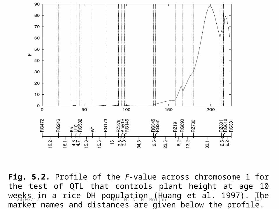
Fig. 5.2. Profile of the F-value across chromosome 1 for the test of QTL that controls plant height at age 10 weeks in a rice DH population (Huang et al. 1997). The marker names and distances are given below the profile.
137Dr. M. N. H. Mollah24/03/12
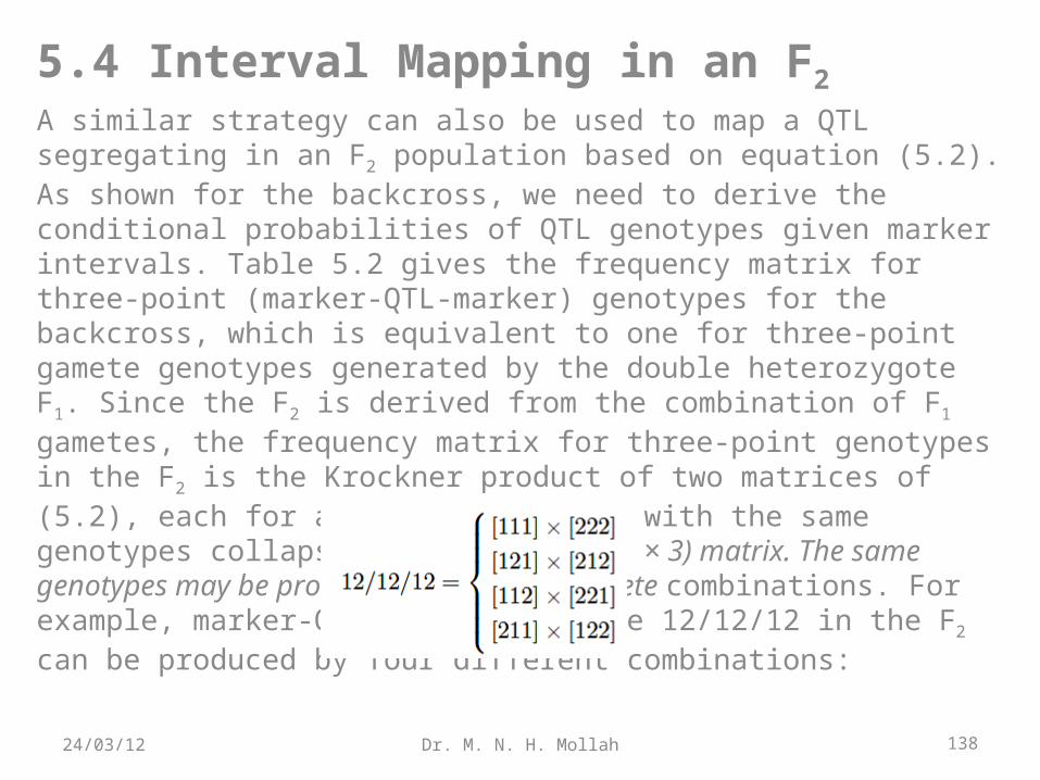
5.4 Interval Mapping in an F2
A similar strategy can also be used to map a QTL segregating in an F2 population based on equation (5.2). As shown for the backcross, we need to derive the conditional probabilities of QTL genotypes given marker intervals. Table 5.2 gives the frequency matrix for three-point (marker-QTL-marker) genotypes for the backcross, which is equivalent to one for three-point gamete genotypes generated by the double heterozygote F1. Since the F2 is derived from the combination of F1 gametes, the frequency matrix for three-point genotypes in the F2 is the Krockner product of two matrices of (5.2), each for a different parent with the same genotypes collapsed to become a (9 × 3) matrix. The same genotypes may be produced by different gamete combinations. For example, marker-QTL-marker genotype 12/12/12 in the F2 can be produced by four different combinations:
138Dr. M. N. H. Mollah24/03/12
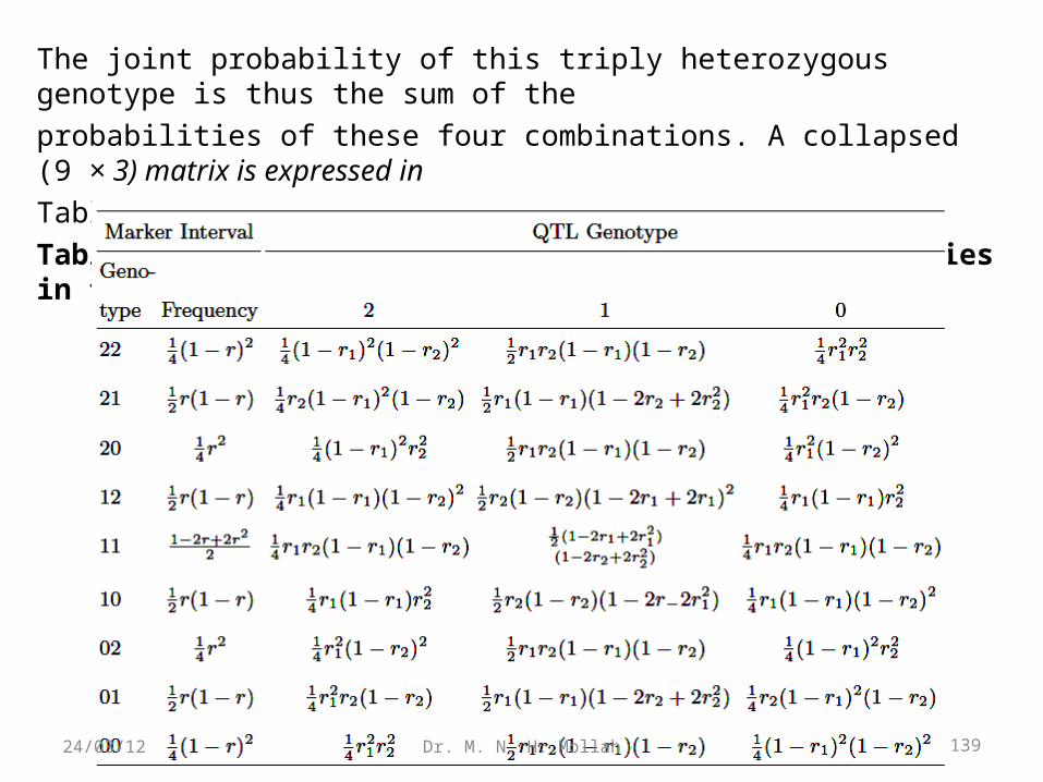
The joint probability of this triply heterozygous genotype is thus the sum of the
probabilities of these four combinations. A collapsed (9 × 3) matrix is expressed in
Table 5.5.
Table 5.5. Joint marker-QTL-marker genotype frequencies in the F2.
139Dr. M. N. H. Mollah24/03/12
From Table 5.5, the coefficients associated with the additive effect (a) and dominant effect (d) of the QTL in the F2 (Table 10.6), which are the explanatory variables, can be derived in terms of the genomic position of a QTL described by the recombination fraction between the QTL and markers. Because the QTL position is unknown, a grid search strategy, in which a QTL is assumed at every position between two markers, is used to regress the trait value on the explanatory variable to calculate μ, a, and d and the F–statistic for the significance of the regression and identify the position with the largest F-value for the regression as the most likely position for a QTL.
Example 5.2. Cheverud et al. (1996) constructed a linkage map using 75 microsatellite markers in a population of 535 F2 progeny derived from two strains, the Large (LG/J) and Small (SM/J). The F2 progeny were measured for body mass at 10 weekly intervals starting at age 7 days. The raw weights were corrected for the effects of each covariate due to dam, litter size at birth and parity but not for the effect due to sex. We use chromosome 1 composed of nine markers to map a QTL affecting body weight at age 10 weeks with LS-based regression approaches.
140Dr. M. N. H. Mollah24/03/12
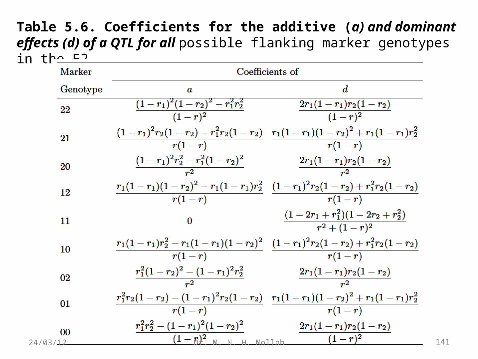
Table 5.6. Coefficients for the additive (a) and dominant effects (d) of a QTL for all possible flanking marker genotypes in the F2.
141Dr. M. N. H. Mollah24/03/12
Figure 5.3 illustrates the profile of the F-values calculated by equation (5.7) at
different positions across a linkage group of chromosome 1 constructed by 18 markers. There is a clear peak at 46 cM in the marker interval [D2MIT389–D2MIT17], whose F-value, 16.434, is largely beyond the critical F0.05,(1,451) = 3.862. This suggests the existence of a significant QTL around that position.
The LS estimates of the model parameters, μ, a, d, and σ2, are obtained at the
peak of the F-value profile. They are ˆμ = 23.0, ˆa = 1.6, ˆ d = 1.4, and ˆσ2 = 21.7. The genetic variance of plant height due to this detected QTL is calculated as σ2
g = 1.5 with equation (4.4). This allows the calculation of the proportion of the phenotypic variance explained by this QTL (R2 = 0.06) with equation (4.5).
Compared with the backcross, the F2 population is more informative because it
allows the significance test of both the additive and dominance effects of a detected
QTL. The full model with the additive effect is written as
142Dr. M. N. H. Mollah24/03/12
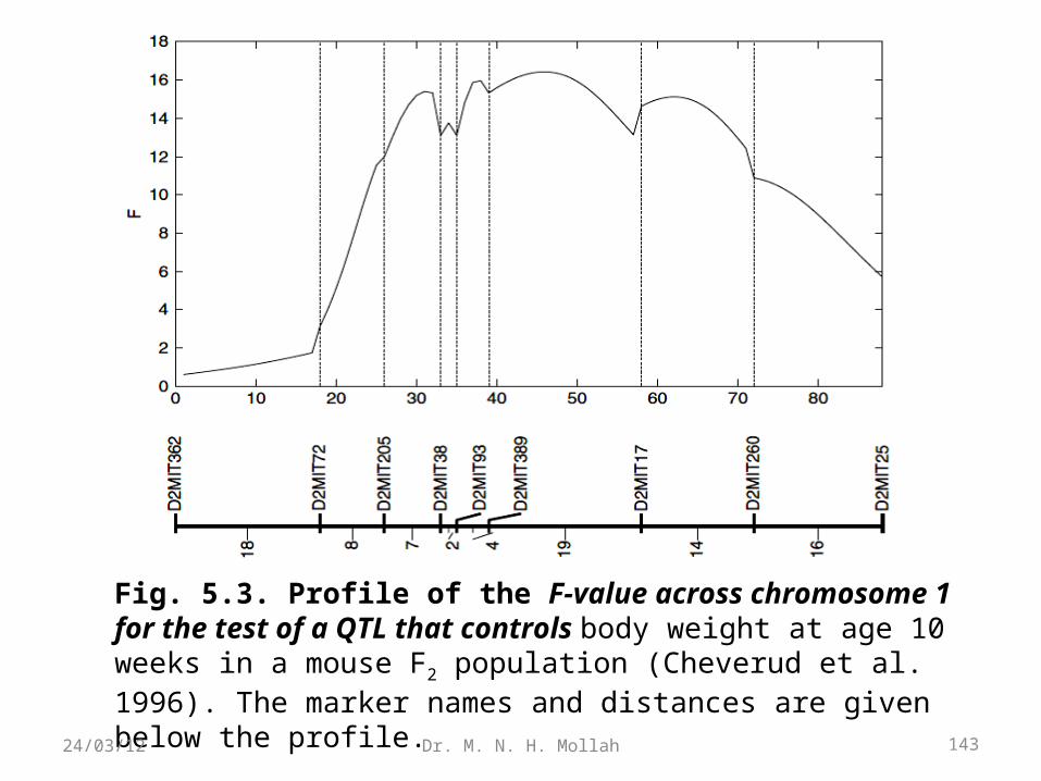
Fig. 5.3. Profile of the F-value across chromosome 1 for the test of a QTL that controls body weight at age 10 weeks in a mouse F2 population (Cheverud et al. 1996). The marker names and distances are given below the profile.
143Dr. M. N. H. Mollah24/03/12
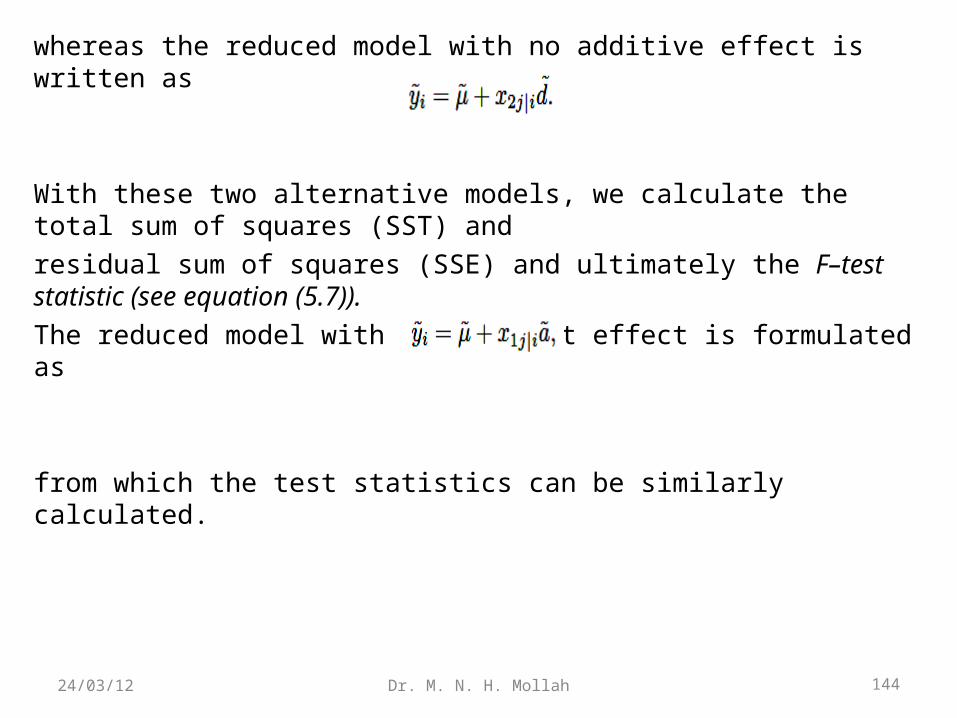
whereas the reduced model with no additive effect is written as
With these two alternative models, we calculate the total sum of squares (SST) and
residual sum of squares (SSE) and ultimately the F–test statistic (see equation (5.7)).
The reduced model with no dominant effect is formulated as
from which the test statistics can be similarly calculated.
144Dr. M. N. H. Mollah24/03/12

THANKS
Dr. M. N. H. Mollah 14524/03/12