Embed Size (px)
Citation preview

WELCOMEWELCOME
EF 105
Fall 2006

EF 105Computer Methods in
Engineering Problem Solving
Week07: Trig Review and Charts
Use of EXCEL
Learning Objectives
Learn more about functionsLearn how to use Trigonometry functionsLearn to use tables and graphs as problem solving toolsLearn and apply different types of graphs and scalesPrepare graphs in ExcelBe able to edit graphs

Use Excel’s functions
Functions TAKE argumentsFunctions RETURN valuesYou can easily calculate the sum, average, count, etc. of a large number of cells by using a function. A function is a predefined, or built-in, formula for a commonly used calculation. Each Excel function has a name and syntax. The syntax specifies the order in which you must
enter the different parts of the function and the location in which you must insert commas, parentheses, and other punctuation
Arguments are numbers, text, or cell references used by the function to calculate a value
Some arguments are optional
1 2( , ,.. )ny f x x x

Work with the Insert Function button
Excel supplies more than 350 functions organized into 10 categories: Database, Date and Time, Engineering, Financial,
Information, Logical, Lookup, Math, Text and Data, and Statistical functions
You can use the Insert Function button on the Formula bar to select from a list of functions. A series of dialog boxes will assist you in filling in the arguments of the function and this process also enforces the use of proper syntax.

Anatomy of Excel Functions
=FUNCTION(argument1,argument2,..,argumentN,…)
optionalMandatory 1..N-1Name

Define functions, and functions within functions
The SUM function is a very commonly used math function in Excel. A basic formula example to add up a small number of cells is =A1+A2+A3+A4, but that method would be cumbersome if there were 100 cells to add up. Use Excel's SUM function to total the values in a range of cells like this: SUM(A1:A100).You can also use functions within functions. Consider the expression =ROUND(AVERAGE(A1:A100),1). This expression would first compute the average of all
the values from cell A1 through A100 and then round that result to 1 digit to the right of the decimal point

Open the Insert Function dialog box
To get help from Excel to insert a function, first click the cell in which you wish to insert the function. Click the Insert Function button. This action will open the Insert Function dialog box. If you do not see the Insert Function button, you may need to select the appropriate toolbar or add the button to an existing toolbar.

Examine the Insert Function dialog box
This dialog box appears when you click the Insert Function button. It can assist you in defining your function.

Use the Insert Function dialog box to enter function arguments
This figure depicts how you would enter argument values for the PMT function using the Insert Function dialog box.
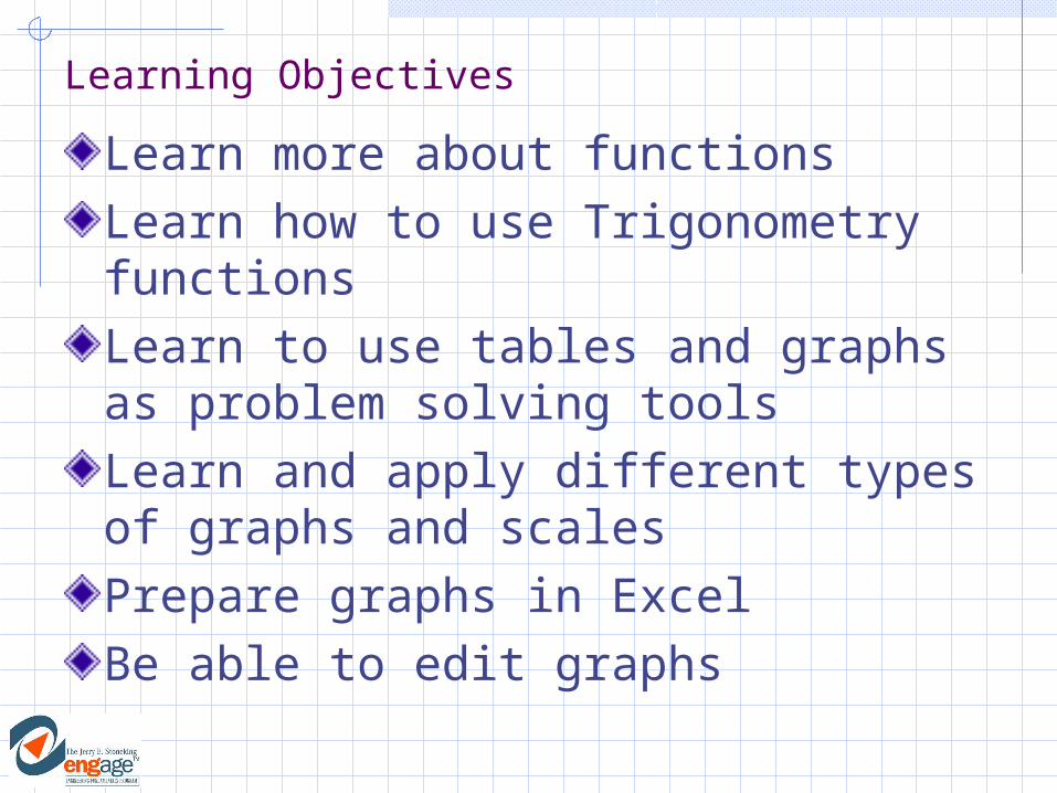
Recognize optional arguments
In the preceding figure, note how rate and nper are arguments for each function.For some of the functions, the final two arguments of each function are in brackets. These represent optional arguments, meaning if you do not enter anything, the default values for these arguments will be used. For example, note the PMT function has fv and type as its final two arguments, which are optional. The assumed values, if no others are supplied, are 0 for both
Arguments without brackets do not have default values, so you must supply values or cell references in order for the function to be able to return a value.
Create logical functions
A function that determines whether a condition is true or false is called a logical function. Excel supports several logical functions such as AND, FALSE, IF, NOT, OR and TRUE. A very common function is the IF function, which uses a logical test to determine whether an expression is true or false, and then returns one value if true or another value if false. The logical test is constructed using a comparison operator that compares two expressions to determine if they are equal, not equal, if one is greater than the other, and so forth. The comparison operators are =, >, >=, <, <=, and <>
You can also make comparisons with text strings. You must enclose text strings within quotation marks.

Using the If function
The arguments for the IF function are: IF(logical_test,value_if_true,value_if_false) For example, the function =IF(A1=10,20,30)
tests whether the value in cell A1 is equal to 10 If it is, the function returns the value 20,
otherwise the function returns the value 30 Cell A1 could be empty or contain anything else
besides the value 10 and the logical test would be false; therefore, the function returns the value 30
To insert an IF function, click the Insert Function button and search for the IF function, then click OK. When the Function Arguments dialog box appears, simply fill in the arguments.

The TODAY and Now functionsThe TODAY and NOW functions always display the current date and time.You will not normally see the time portion unless you have formatted the cell to display it.If you use the TODAY or NOW function in a cell, the date in the cell is updated to reflect the current date and time of your computer each time you open the workbook.
Let’s open your saved workbooks from last class and add a logical and a date function!

Use a formula to enter the dateIf you wanted a fixed date to remain in a cell , you would enter that date. If you wanted the date in this cell to always reflect the current date and time when you opened the workbook, you would use the expression =NOW() or =TODAY() as shown in the formula bar in the figure.

TRIGONOMETRY FUNCTIONS
When solving trigonometric expressions like sine, cosine and tangent, it is very important to realize that Excel uses radians, not degrees to perform these calculations! If the angle is in degrees you must first convert it to radians. There are two easy ways to do this.
1.Recall that = 180°. Therefore, if the angle is in degrees, multiply it by /180° to convert it to radians. With Excel, this conversion can be written PI( )/180. For example, to convert 45° to radians, the Excel expression would be 45*PI( )/180 which equals 0.7854 radians. 2.Excel has a built-in function known as RADIANS(angle) where angle is the angle in degrees you wish to convert to radians. For example, the Excel expression used to convert 270° to radians would be RADIANS(270) which equals 4.712389 radians

TRIGONOMETRY FUNCTIONS
You can use the DEGREES(angle) function to convert radians into degrees. For example, DEGREES(PI( ) ) equals 180.
Excel uses several built-in trig functions. Those that you will use most often are displayed in the table below. Note that the arguments for the SIN( ), COS( ) and TAN( ) functions are, by default, radians. Also, the functions ASIN( ), ACOS( ) and ATAN( ) return values in terms of radians. (When working with degrees, you will need to properly use the DEGREES( ) and RADIANS( ) functions to convert to the correct unit.)

TRIGONOMETRY FUNCTIONS
Mathematical Expression
Excel Expression
Excel Examples
sine: sin() SIN(number) SIN(30) equals -0.98803, the sine of 30 radians
SIN(RADIANS(30)) equals 0.5, the sine of 30°
cosine: cos() COS(number) COS(1.5) equals 0.07074, the cosine of 1.5 radians
COS(RADIANS(1.5)) equals 0.99966, the sine of 1.5°
tangent: tan() TAN(number) TAN(2) equals -2.18504, the tangent of 2 radians
TAN(RADIANS(2)) equals 0.03492, the tangent of 2°
arcsine: sin-1(x) ASIN(number) ASIN(0.5) equals 0.523599 radians
DEGREES(ASIN(0.5)) equals 30°, the arcsine of 0.5
arccos: cos-1(x) ACOS(number) ACOS(-0.5) equals 2.09440 radians
DEGREES(ACOS(-0.5)) equals 120°, the arccosine of -0.5
arctangent: tan-
1(x) ATAN(number) ATAN(1) equals 0.785398 radians
DEGREES(ATAN(1)) equals 45°, the arctangent of 1
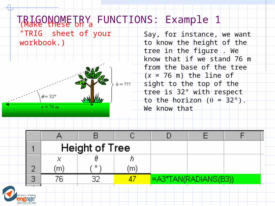
TRIGONOMETRY FUNCTIONS: Example 1Say, for instance, we want to know the height of the tree in the figure . We know that if we stand 76 m from the base of the tree (x = 76 m) the line of sight to the top of the tree is 32° with respect to the horizon ( = 32°). We know that
Solving for the height of the tree, h, we find
(Make these on a “TRIG” sheet of your workbook.)

TRIGONOMETRY FUNCTIONS: Example 2
In this next example, we wish to know the launch angle, , of the water ski ramp shown. We are given that A = 3.5 m, B = 10.2 m and = 45.0°. To find , we can use the Law of Sines which, in this case can be written
We can rewrite this equation as using the equation
The screen shot below shows how we used Excel to determine that the launch angle of the ramp is 14.04°.

TRIGONOMETRY FUNCTIONS: Example #3
In our final trigonometry example, we will use Excel to examine the trig identity
Notice in the screen shot below that this identity holds true when is given in radians and degrees. Note the units for the angle are placed in different cells than the numbers. If we place the numbers and the units in the same cell, Excel will not be able to decipher the number and therefore we will not be able to reference the cells for use in any equation!

Proper Use of Tables & Graphs
Engineers record and present data in two primary formats: Tables and Graphs
Height H (m)
Temp T (C)
Pressure P (kPa)
0 15.0 101.3 300 12.8 97.7
600 11.1 94.2
0
2
4
6
8
10
12
14
16
0 500 1000 1500Height (m)
Tem
per
atu
re (
C)
0
20
40
60
80
100
120
140
160
Pre
ssu
re (
kPa)
Temp
Pressure
(Make these on a “TCG” sheet of your workbook.)

Tables
Tables should always have: Title Column headings with brief descriptive name,
symbol and appropriate units.
Numerical data in the table should be written to the proper number of significant digits. The decimal points in a column should be
aligned.
Tables should always be referenced and discussed (at least briefly) in the body of the text of the document containing the table.

Table Example
Temperature and Pressure ofWidgets at Various Heights
Height H (m)
Temp T (C)
Pressure P (kPa)
0 15.0 101.3 300 12.8 97.7 600 11.1 94.2

ExerciseEnter the following table in Excel (Label a sheet in the workbook you’ve been using in class.)
You can make your tables look nice by formatting text and borders
Independent Variable, x
Dependent Variable, y1
Dependent Variable, y2
1 1 1
2500 10 50 5000 100 100
7500 1000 150
10000 10000 200

Graphs
Proper graphing of data involves several steps: Select appropriate graph type Select scale and gradation of axes, and
completely label axes Plot data points, then plot or fit curves Add titles, notes, and or legend

Graphs - Types
Travel Expenses
02468
1012141618
Fo
od
Ga
s
Mo
tel
Exp
ense
s ($
)
1. Pie Chart 2. Bar Graph

Graphs - Types
4. Line Graph
0
2
4
6
8
10
12
14
16
0 500 1000 1500Height (m)
Tem
per
atu
re (
C)
0
20
40
60
80
100
120
140
160
Pre
ssu
re (
kPa)
Temp
Pressure
1
2
3
4
5
6
7
01234567
8
02468101214
Object 1Object 2
Bod
y T
emp
erat
ure
(0C
Speed (m/s) Dis
tanc
e (m
)
3. 3-D Graph

Graphs
Each graph must include: A descriptive title which provides a clear and
concise statement of the information being presented
A legend defining point symbols or line types used for curves needs to be included
Labeled axes
Graphs should always be referenced/discussed in the body of the text of the document containing the table.

Titles and Legends
Each graph must be identified with a descriptive titleThe title should include clear and concise statement of the information being presentedA legend defining point symbols or line types used for curves needs to be included

Axis Labels
Each axis must be labeledThe axis label should contain the name of the variable and its units. The units can be enclosed in parentheses, or separated from the label by a comma.
Length (km)

Gradation
Scale gradations should be selected so that the smallest division of the axis is an integer power of 10 times 1, 2, or 5. Exception is units of time.
Scale Graduations,Smallest Division=1
Acceptable
Scale Graduations,Smallest Division=3.33
Not Acceptable
Data Points and Curves
Data Points are plotted using symbols The symbol size must be large enough to
easily distinguish them A different symbol is used for each data set
Data Points are often connected with lines A different line style is often used for each
data set

Example
Velocity of Three RunnersDuring a 5 km Race

Building a Graph In Excel
Select the data that you want to include in the chart by dragging through it with the mouse.Then click the Chart Wizard

Choose XY (Scatter), with data connected by lines if desired.Click “Next”
Building the Graph

Building the Graph
Make sure that the series is listed in columns, since your data is presented in columns.Click the Series tab to enter a name for the data set, if desired.Choose “Next”

Building the Graph
Fill in Title and Axis information“Next”

Building a Chart
Select “As new sheet” to create the chart on it’s own sheet in your Excel file, or “As object in” to create the chart on an existing sheet“Finish”

Creating a Secondary Axis
This is useful when the data sets cover very different ranges.Right click on the line (data series) on the chart that you want to associate with a secondary axis.Select “format data series”Select the Axis tab, then “Plot series on secondary axis” as shown.“OK”
Editing/Adding Labels
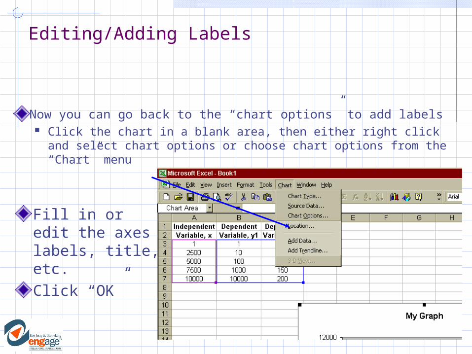
Now you can go back to the “chart options” to add labels Click the chart in a blank area, then either right click and
select chart options or choose chart options from the “Chart” menu
Fill in or edit the axes labels, title, etc.Click “OK”

Result

A Baseball Problem
A runner is on 3rd base, 90 ft from home plate. He can run with an average speed of 27 ft/s. A ball is hit to the center fielder who catches it 310 ft from home plate. The center fielder can throw the ball no faster than 110 ft/s. The runner tags up and runs for home plate.
Can the center fielder throw him out? To do so, he must get the ball to the catcher at an appropriate height before the runner can get to home plate.
If so, at what angle and what velocity does he need to throw the ball in order to put the runner out?
(Make these on a “Baseball” sheet of your workbook.)

Graphic Translation
Runner
90 ft
tvttr
s
ft27)(
Center Fielder
310 ft
jgttVty
20 2
1)sin()(
itVtx
)cos()( 0
V0
j
i

Solving with Excel-Iteration Method
Open an Excel spreadsheet and create column heads like the example.Rows 1 - 6 are for constants. Remember to use the $ notation when reference absolute address

Solutions - Building a Table
Rows 7 and above can be used to calculate the x and y positions at different times t using the formula for projectile motion. For example, under x(t) in Cell B8 enter the formula:
= $B$4*cos($C$2)*A8What formula would be entered for y(t) (height)and r(t) (runner position)?Is there an easy way to enter the values for time beginning in Cell A8?

Solution - iterations
Notice how changing Cell B2 effects the rest of the spreadsheet, especially x(t) and y(t) columns.
By watching the results in those columns, you can get arbitrarily close to 310 and 0. Also Cell B4 can be changed for even finer tuning.

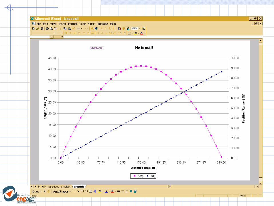
Solution - Using a Chart
Another way to solve this problem is with a graph. This method will use the data generated on the previous slides but will use a chart to show the result.The next slide shows a completed chart. Notice that the line shows the ball position reaches 310 ft before the runner has traveled 90 ft.

Building a Chart (Step 1)
Select the data that you want to include in the chart by dragging through it with the mouse.

Building a Chart (Step 2)
click the chart wizard.

Choose XY (Scatter) Then choose “Next”
Building a Chart (Step 3)

Building a Chart (Step 4)
Make sure that the series is listed in columns.Choose “Next”

Building a Chart (Step 5)
Fill in Title and Axis information
“Next”

Building a Chart (Step 6)
Choose “As new sheet”, then “Finish”

Building a Chart (Step 7)
Creating a Secondary axis. Right click on the data
series that you want to associate with a secondary axis.
Right click and choose “format data series.
Select “Plot series on secondary axis”

Building a Chart (Step 8)
Select “Chart”, then “Chart Options”Fill in the title for secondary value (Y) axis.Click “OK”This should complete the chart.

Using Solver
Select and copy the first 8 rows of the first 4 columns of the spread sheet.Remember that Row 8 contains the formulas for calculating the x, y and r positions.

Using Solver
Select another worksheet from the bottom of the spreadsheetRight click on its label and rename if desired.Select Cell A1Paste.

Using Solver
Pull down Tools, then select solver.
Set Target CellDesired ValueManipulated
Cells Constraints
Select Solve

Using Solver
Solver arrives at a solution that is within the constraints. = 28.31 degreesV0 = 110 ft/s
t = 3.20 seconds.The ball is at home plate two feet off the ground while the runner is still 3.58 feet away.
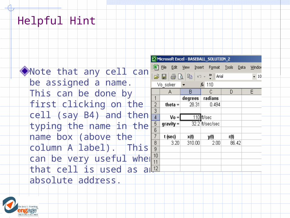
Helpful Hint
Note that any cell can be assigned a name. This can be done by first clicking on the cell (say B4) and then typing the name in the name box (above the column A label). This can be very useful when that cell is used as an absolute address.

Helpful HintThe name can then be used when typing formulas. This creates a formula that looks more like the actual equation making it easier to type and to verify. In this example the cell names, Vo_solver, theta_solver, and time were used instead of $B$4, $C$2, $A$8.

Next,
1. Do the Tutorial, Part 2
on your own
2. Solve the following on your own:
A. What is the length of horizontal base of the triangle? (cm)B. What is the area of this triangle? (sq. cm)