Weil Diffeology I: Classical DifferentialGeometry

著者 NISHIMURA Hirokazupage range 1-21year 2017-02-21URL http://hdl.handle.net/2241/00145317

arX

iv:1

702.

0576

9v2

[m

ath.

CT

] 2

1 Fe

b 20

17

Weil Diffeology I:

Classical Differential Geometry

Hirokazu NISHIMURA

Institute of Mathematics, University of Tsukuba

Tsukuba, Ibaraki 305-8571

Japan

February 22, 2017

Abstract

Topos theory is a category-theoretical axiomatization of set theory.Model categories are a category-theoretical framework for abstract ho-motopy theory. They are complete and cocomplete categories endowedwith three classes of morphisms (called fibrations, cofibrations and equiv-alences) satisfying certain axioms. Functors from the category W of Weilalgebras to the category Sets of sets are called Weil spaces by WolfgangBertram and form the Weil topos after Eduardo J. Dubuc. The Weiltopos is endowed intrinsically with the Dubuc functor, a functor froma larger category W to the Weil topos standing for the incarnation ofeach algebraic entity of W in the Weil topos. The Weil functor and thecanonical ring object are to be defined in terms of the Dubuc functor.The principal object in this paper is to present a category-theoretical ax-iomatization of the Weil topos with the Dubuc functor intended to bean adequate framework for axiomatic classical differential geometry andhopefully comparable with model categories. We will give an appropriateformulation and a rather complete proof of a generalization of the familiarand desired fact that the tangent space of a microlinear Weil space is amodule over the ring object.

1 Introduction

Differential geometry usually exploits not only the techniques of differentiationbut also those of integration. In this paper we would like to use the term ”dif-ferential geometry” in its literal sense, that is, genuinely differential geometry,which is large enough as to encompass a large portion of the theory of connec-tions and the core of the theory of Lie groups. Now we know well that there isa horribly deep and overwhelmingly gigantic valley between differential calculusof the 17th and 18th centuries, say, that of the good old days of Newton, Leib-niz, Lagrange, Laplace, Euler and so on, and that of our modern age since the

1

19th century when Angustin Louis Cauchy was active. The former exquisitelyresorts to nilpotent infinitesimals, while the latter grasps differentiation in termsof limits by using so-called ε−δ arguments formally. Differential geometry basedon the latter style of differentiation is generally called smootheology, while wepropose that differential geometry based on the former style of differentiationmight be called Weilology.

As is well known, the category of topological spaces and continuous mappinsis not cartesian closed. The classical example of a convenient category of topo-logical spaces for working topologisits was suggested by Norman Steenrod [33]in the middle of the 1960s, namely, the category of compactly generated spaces.Now the category of finite-dimensional smooth manifolds and smooth mappingsis not cartesian closed, either. Convenient categories for smootheology havebeen proposed by several authors in several corresponding forms. Among themSouriau’s [31] approach based upon the category O of open subsets O’s of Rn’sand smooth mappings between them has developed into a galactic volume ofdiffeology, for which the reader is referred to [9]. A diffeological space is a set Xendowed with a subset D (O) ⊆ XO for each O ∈ O such that, for any morphismf : O → O′ in O and any γ ∈ D (O′), we have γ ◦ f ∈ D (O). A diffeologicalmap between diffeological spaces (X,D) and (X,D′) is a mapping f : X → X ′

such that, for any O ∈ O and any γ ∈ D (O), we have f ◦ γ ∈ D′ (O).Roughly speaking, there are two approaches to geometry in representing

spaces, namely, contravariant (functional) and covariant (parameterized) ones,for which the reader is referred, e.g., to Chapter 3 of [30] as well as [24] and [25].Diffeology finds itself in the covariant realm. The contravariant approach boilsdown spaces to their function algebras. We are now accustomed to admitting allalgebras to stand for abstract spaces in some way or other, whatever they maybe. This is a long tradition of algebraic geometry since as early as AlexanderGrothendieck. Now we are ready to acknowledge any functor Oop → Sets asan abstract diffeological space. Then it is pleasant to enjoy

Theorem 1 The category of abstract diffeological spaces and natural transfor-mations between them is a topos.

Turning to Weilology, a space should be represented as a functor Infop →

Sets, where Inf stands for the category of nilpotent infinitesimal spaces. Sinceour creed tells us that the category Infop is equivalent to W, a space should beno other than a functor W→ Sets, for which Wolfgang Bertram [6] has coinedthe term ”Weil space”. Surely we have

Theorem 2 The category of Weil spaces and natural transformations betweenthem is a topos.

2 An Extension of Weil Algebras

Unless stated to the contrary, our base field is assumed to be R (real numbers)throughout the paper, so that we will often say ”Weil algebra” simply in place

2

of Weil R-algebra”. For the exact definition of a Weil algebra, the reader isreferred to §I.16 of [10].

Notation 3 We denote by W the category of Weil algebras.

Remark 4 R is itself a Weil algebra, and it is an initial object in the categoryW.

Definition 5 AnR-algebra isomorphic to an R-algebra of the form R [X1, ..., Xn]⊗W with R [X1, ..., Xn] being the polynomial algebra over R in indeterminatesX1, ..., Xn (possibly n = 0) andW being a Weil algebra is called a quasi-Weil algebra.

Remark 6 This definition of a quasi-Weil algebra is reminiscent of that in thedefinition of Cahiers topos, where we consider a product of a Cartesian spaceRn and a formal dual of a Weil algebra.

Notation 7 We denote by W the category of quasi-Weil algebras.

Remark 8 The category W is a full subcategory of the category W. Both areclosed under the tensor product ⊗.

Notation 9 We will use such a self-explanatory notation as Z → X/(X2

)or

X/(X2

)← Z for the morphism R [Z] → R [X ] /

(X2

)assigning X modulo(

X2)to Z.

3 Weil Spaces

Definition 10 A Weil space is simply a functor F from the category W of Weilalgebras to the category Sets of sets. A Weil morphism from a Weil space F toanother Weil space G is simply a natural transformation from the functor F tothe functor G.

Remark 11 The term ”Weil space” has been coined in [6].

Example 12 The Weil prolongation of a ”manifold” in its broadest sense (cf.[4]) by a Weil algebra was fully discussed by Bertram and Souvay, for whichthe reader is cordially referred to [5]. We are happy to know that any manifoldnaturally gives rise to its associated Weil space, which can be regarded as afunctor from the category of manifolds to the category Weil. It should be stressedwithout exaggeration that the functor is not full in general, for which the readeris referred to exuberantly readable §1.6 (discussion) of [6].

Example 13 The Weil prolongation A ⊗W of a C∞-algebra A by a Weil al-gebra W was discussed in Theorem III.5.3 of [10]. We are happy to know thatany C∞-algebra naturally gives rise to its associated Weil space.

Notation 14 We denote by Weil the category of Weil spaces and Weil mor-phisms.

3

Remark 15 Dubuc [7] has indeed proposed the topos Weil as the first steptowards the well adapted model theory of synthetic differential geometry, but wewould like to contend somewhat radically that the topos Weil is verbatim thecentral object of study in classical differential geometry

It is well known (cf. Chapter 1 of [14]) that

Theorem 16 The category Weil is a topos. In particular, it is locally cartesianclosed.

Remark 17 Dubuc [7] has called the category Weil the Weil topos.

Remark 18 The category of Frolicher spaces is indeed cartesian closed, but itis not locally cartesian closed. On the other hand, the category of diffeologicalspaces is locally cartesian closed. For these matters, the reader is referred to[?]. It was shown by Baez and Hoffnung [2] that diffeological spaces as well asChen spaces are no other than concrete sheaves on concrete sites.

Definition 19 The Weil prolongation FW of a Weil space F by a Weil algebraW is simply the composition of the functor ( ) ⊗W : W →W and the functorF : W→ Sets, namely

F (( )⊗W ) : W→ Sets

which is surely a Weil space.

Remark 20 ( )(·)

assigning FW to each (W,F ) ∈W ×Weil can naturally beregarded as a bifunctor W×Weil→Weil.

Trivially we have

Proposition 21 For any Weil space F and any Weil algebras W1 and W2, wehave (

FW1)W2

= FW1⊗W2

Remark 22 The so-called Yoneda embedding

y : Wop →Weil

is full and faithful. The famous Yoneda lemma claims that

F ( ) ∼= HomWeil (y ( ) , F ) (1)

for any Weil space F . The Yoneda embedding can be extended to

y : Wop →Weil

byy (A) = HomR−Alg (A, )

for any A ∈ W, where R−Alg denotes the category of R-algebras.

4

Remark 23 Given Weil algebras W1 and W2, we have

yW1 × yW2∼= y (W1 ⊗W2) (2)

Remark 24 As is well known (cf. §8.7 of [1]), given Weil spaces F and G,their exponential FG in Weil is provided by

HomWeil (y ×G,F ) (3)

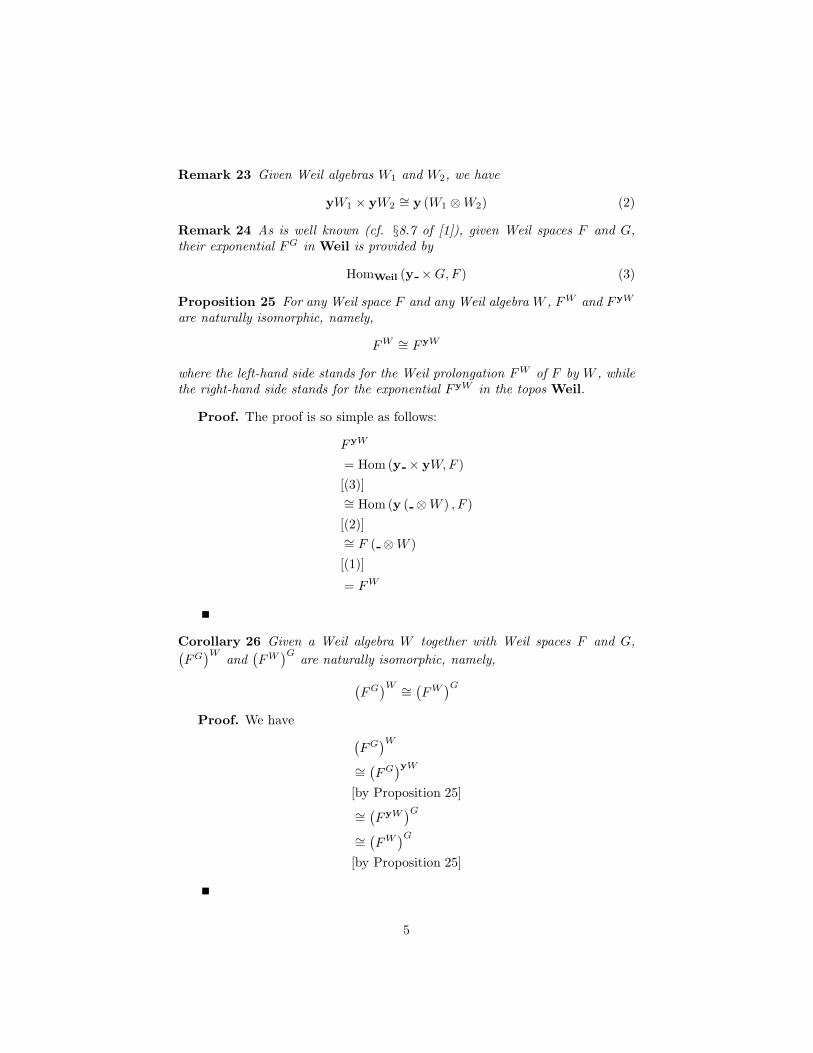
Proposition 25 For any Weil space F and any Weil algebra W , FW and FyW

are naturally isomorphic, namely,

FW ∼= FyW

where the left-hand side stands for the Weil prolongation FW of F by W , whilethe right-hand side stands for the exponential FyW in the topos Weil.

Proof. The proof is so simple as follows:

FyW

= Hom(y × yW,F )

[(3)]∼= Hom(y ( ⊗W ) , F )

[(2)]∼= F ( ⊗W )

[(1)]

= FW

Corollary 26 Given a Weil algebra W together with Weil spaces F and G,(FG

)Wand

(FW

)Gare naturally isomorphic, namely,

(FG

)W ∼=(FW

)G

Proof. We have

(FG

)W

∼=(FG

)yW

[by Proposition 25]

∼=(FyW

)G

∼=(FW

)G

[by Proposition 25]

5

Corollary 27 For any Weil algebra W , the functor ( )W

: Weil →Weil pre-serves limits, particularly, products.

Proof. Since the functor ( )W is of its left adjoint ( )×yW (cf. Proposition8.13 of [1]), the desired result follows readily from the well known theoremclaiming that a functor being of its left adjoint preserves limits (cf. Proposition9.14 of [1]).

Notation 28 We denote by R the forgetful functor W→ Sets, which is surelya Weil space. It can be defined also as

R = y (R [X ])

Remark 29 The Weil space R is canonically regarded as an R-algebra objectin the category Weil.

Remark 30 Since R is an R-algebra object in the category Weil, we can define,after §I.16 of [10], another R-algebra object R ⊗W in the category Weil forany Weil algebra W .

Notation 31 We denote by R−Alg (Weil) the category of R-algebra objectsin the category Weil.

Proposition 32 The functors

Ry( ),R⊗ ( ) : W→ R−Alg (Weil)

are naturally isomorphic.

Proof. We have

RyW (W ′)

∼= RW (W ′)

[By Proposition 25]

=W ′ ⊗W

4 Microlinearity

Not all Weil spaces are susceptible to the techniques of classical differentialgeometry, so that there should be a criterion by which we can select decentones.

Definition 33 A Weil space F is called microlinear provided that a finite limitdiagram D in W always yields a limit diagram FD in Weil.

6

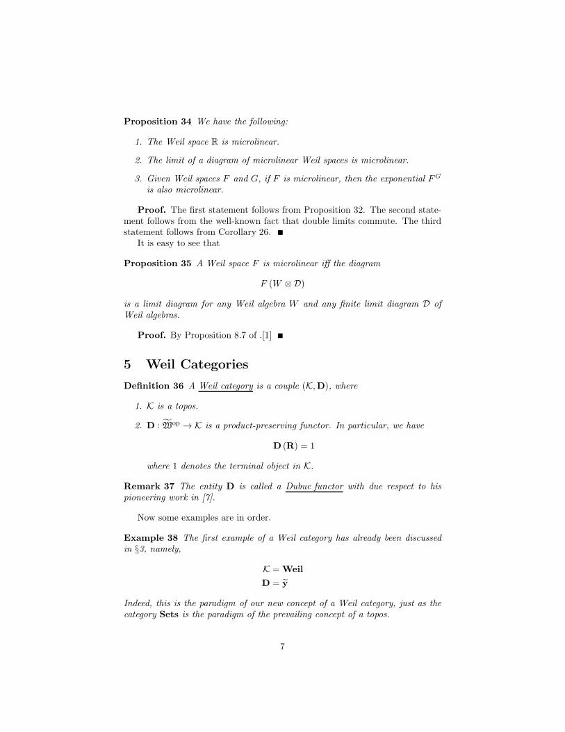
Proposition 34 We have the following:

1. The Weil space R is microlinear.

2. The limit of a diagram of microlinear Weil spaces is microlinear.

3. Given Weil spaces F and G, if F is microlinear, then the exponential FG

is also microlinear.

Proof. The first statement follows from Proposition 32. The second state-ment follows from the well-known fact that double limits commute. The thirdstatement follows from Corollary 26.

It is easy to see that

Proposition 35 A Weil space F is microlinear iff the diagram

F (W ⊗D)

is a limit diagram for any Weil algebra W and any finite limit diagram D ofWeil algebras.

Proof. By Proposition 8.7 of .[1]

5 Weil Categories

Definition 36 A Weil category is a couple (K,D), where

1. K is a topos.

2. D : Wop → K is a product-preserving functor. In particular, we have

D (R) = 1

where 1 denotes the terminal object in K.

Remark 37 The entity D is called a Dubuc functor with due respect to hispioneering work in [7].

Now some examples are in order.

Example 38 The first example of a Weil category has already been discussedin §3, namely,

K = Weil

D = y

Indeed, this is the paradigm of our new concept of a Weil category, just as thecategory Sets is the paradigm of the prevailing concept of a topos.

7

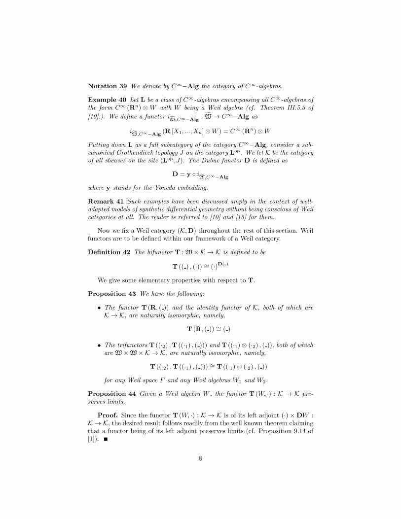
Notation 39 We denote by C∞−Alg the category of C∞-algebras.

Example 40 Let L be a class of C∞-algebras encompassing all C∞-algebras ofthe form C∞ (Rn) ⊗W with W being a Weil algebra (cf. Theorem III.5.3 of

[10].). We define a functor iW,C∞−Alg

: W→ C∞−Alg as

iW,C∞−Alg

(R [X1, ..., Xn]⊗W ) = C∞ (Rn)⊗W

Putting down L as a full subcategory of the category C∞−Alg, consider a sub-canonical Grothendieck topology J on the category Lop. We let K be the categoryof all sheaves on the site (Lop, J). The Dubuc functor D is defined as

D = y ◦ iW,C∞−Alg

where y stands for the Yoneda embedding.

Remark 41 Such examples have been discussed amply in the context of well-adapted models of synthetic differential geometry without being conscious of Weilcategories at all. The reader is referred to [10] and [15] for them.

Now we fix a Weil category (K,D) throughout the rest of this section. Weilfunctors are to be defined within our framework of a Weil category.

Definition 42 The bifunctor T : W×K → K is defined to be

T (( ) , (·)) ∼= (·)D( )

We give some elementary properties with respect to T.

Proposition 43 We have the following:

• The functor T (R, ( )) and the identity functor of K, both of which areK → K, are naturally isomorphic, namely,

T (R, ( )) ∼= ( )

• The trifunctors T ((·2) ,T ((·1) , ( ))) and T ((·1)⊗ (·2) , ( )), both of whichare W×W×K → K, are naturally isomorphic, namely,

T ((·2) ,T ((·1) , ( ))) ∼= T ((·1)⊗ (·2) , ( ))

for any Weil space F and any Weil algebras W1 and W2.

Proposition 44 Given a Weil algebra W , the functor T (W, ·) : K → K pre-serves limits.

Proof. Since the functor T (W, ·) : K → K is of its left adjoint (·) ×DW :K → K, the desired result follows readily from the well known theorem claimingthat a functor being of its left adjoint preserves limits (cf. Proposition 9.14 of[1]).

8

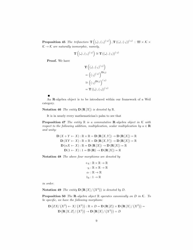
Proposition 45 The trifunctors T(( ) , (·1)

(·2)),T (( ) , (·1))

(·2) : W × K ×

K → K are naturally isomorphic, namely,

T(( ) , (·1)

(·2))∼= T (( ) , (·1))

(·2)

Proof. We have

T(( ) , (·1)

(·2))

=((·1)

(·2))D( )

∼=((·1)

D( ))(·2)

= T (( ) , (·1))(·2)

An R-algebra object is to be introduced within our framework of a Weilcategory.

Notation 46 The entity D (R [X ]) is denoted by R.

It is in nearly every mathematician’s palm to see that

Proposition 47 The entity R is a commutative R-algebra object in K withrespect to the following addition, multiplication, scalar multiplication by α ∈ R

and unity:

D (X + Y ← X) : R× R = D (R [X,Y ])→ D (R [X ]) = R

D (XY ← X) : R× R = D (R [X,Y ])→ D (R [X ]) = R

D (αX ← X) : R = D (R [X ])→ D (R [X ]) = R

D (1← X) : 1 = D (R)→ D (R [X ]) = R

Notation 48 The above four morphisms are denoted by

+R : R× R→ R

·R : R× R→ R

α· : R→ R

1R : 1→ R

in order.

Notation 49 The entity D(R [X ] /

(X2

))is denoted by D.

Proposition 50 The R-algebra object R operates canonically on D in K. Tobe specific, we have the following morphism:

D(ZX/

(X2

)← X/

(X2

)): R×D = D (R [Z])×D

(R [X ] /

(X2

))=

D(R [X,Z] /

(X2

))→ D

(R [X ] /

(X2

))= D

9

Notation 51 The above morphism is denoted by ·R,D.

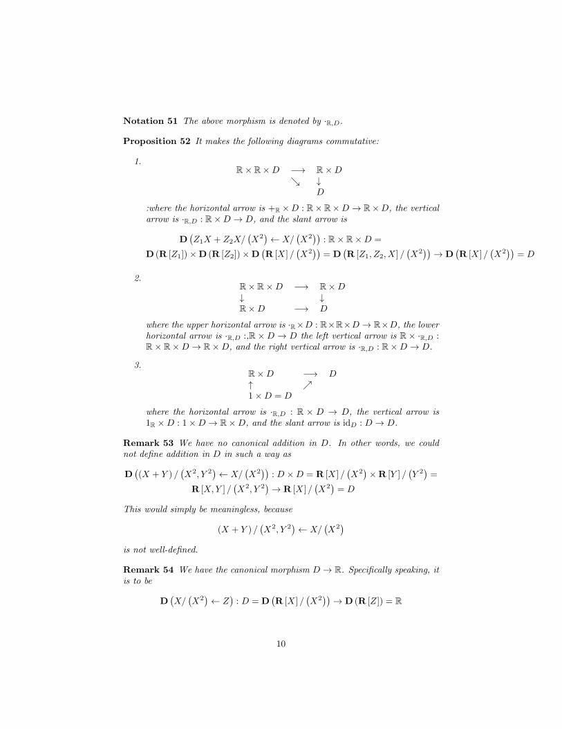
Proposition 52 It makes the following diagrams commutative:

1.R× R×D −→ R×D

ց ↓

D

:where the horizontal arrow is +R ×D : R×R×D → R×D, the verticalarrow is ·R,D : R×D → D, and the slant arrow is

D(Z1X + Z2X/

(X2

)← X/

(X2

)): R× R×D =

D (R [Z1])×D (R [Z2])×D(R [X ] /

(X2

))= D

(R [Z1, Z2, X ] /

(X2

))→ D

(R [X ] /

(X2

))= D

2.R× R×D −→ R×D↓ ↓

R×D −→ D

where the upper horizontal arrow is ·R×D : R×R×D→ R×D, the lowerhorizontal arrow is ·R,D :,R ×D → D the left vertical arrow is R× ·R,D :R× R×D → R×D, and the right vertical arrow is ·R,D : R×D → D.

3.R×D −→ D↑ ր

1×D = D

where the horizontal arrow is ·R,D : R × D → D, the vertical arrow is1R ×D : 1×D → R×D, and the slant arrow is idD : D → D.

Remark 53 We have no canonical addition in D. In other words, we couldnot define addition in D in such a way as

D((X + Y ) /

(X2, Y 2

)← X/

(X2

)): D ×D = R [X ] /

(X2

)×R [Y ] /

(Y 2

)=

R [X,Y ] /(X2, Y 2

)→ R [X ] /

(X2

)= D

This would simply be meaningless, because

(X + Y ) /(X2, Y 2

)← X/

(X2

)

is not well-defined.

Remark 54 We have the canonical morphism D → R. Specifically speaking, itis to be

D(X/

(X2

)← Z

): D = D

(R [X ] /

(X2

))→ D (R [Z]) = R

10

Many significant concepts and theorems of topos theory can quite easily betransferred into the theory of Weil categories surely with due modifications. Inparticular, we have

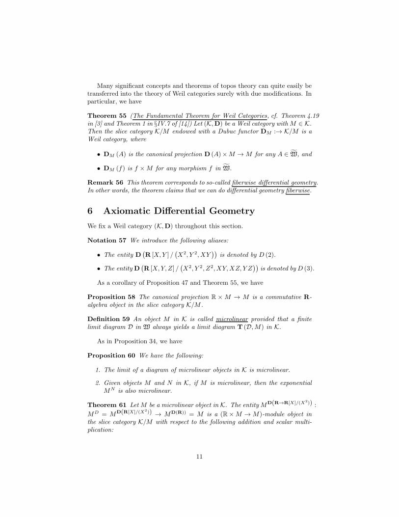
Theorem 55 (The Fundamental Theorem for Weil Categories, cf. Theorem 4.19in [3] and Theorem 1 in §IV.7 of [14]) Let (K,D) be a Weil category withM ∈ K.Then the slice category K/M endowed with a Dubuc functor DM :→ K/M is aWeil category, where

• DM (A) is the canonical projection D (A)×M →M for any A ∈ W, and

• DM (f) is f ×M for any morphism f in W.

Remark 56 This theorem corresponds to so-called fiberwise differential geometry.In other words, the theorem claims that we can do differential geometry fiberwise.

6 Axiomatic Differential Geometry

We fix a Weil category (K,D) throughout this section.

Notation 57 We introduce the following aliases:

• The entity D(R [X,Y ] /

(X2, Y 2, XY

))is denoted by D (2).

• The entityD(R [X,Y, Z] /

(X2, Y 2, Z2, XY,XZ, Y Z

))is denoted by D (3).

As a corollary of Proposition 47 and Theorem 55, we have

Proposition 58 The canonical projection R ×M → M is a commutative R-algebra object in the slice category K/M .

Definition 59 An object M in K is called microlinear provided that a finitelimit diagram D in W always yields a limit diagram T (D,M) in K.

As in Proposition 34, we have

Proposition 60 We have the following:

1. The limit of a diagram of microlinear objects in K is microlinear.

2. Given objects M and N in K, if M is microlinear, then the exponentialMN is also microlinear.

Theorem 61 LetM be a microlinear object in K. The entityMD(R→R[X]/(X2)) :

MD = MD(R[X]/(X2)) → MD(R)) = M is a (R×M →M)-module object inthe slice category K/M with respect to the following addition and scalar multi-plication:

11

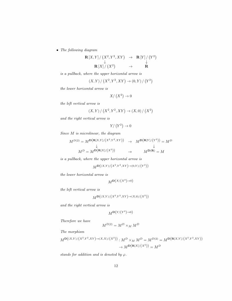
• The following diagram

R [X,Y ] /(X2, Y 2, XY

)→ R [Y ] /

(Y 2

)

↓ ↓

R [X ] /(X2

)→ R

is a pullback, where the upper horizontal arrow is

(X,Y ) /(X2, Y 2, XY

)→ (0, Y ) /

(Y 2

)

the lower horizontal arrow is

X/(X2

)→ 0

the left vertical arrow is

(X,Y ) /(X2, Y 2, XY

)→ (X, 0) /

(X2

)

and the right vertical arrow is

Y/(Y 2

)→ 0

Since M is microlinear, the diagram

MD(2) =MD(R[X,Y ]/(X2,Y 2,XY )) → MD(R[Y ]/(Y 2)) =MD

↓ ↓

MD =MD(R[X]/(X2)) → MD(R) =M

is a pullback, where the upper horizontal arrow is

MD((X,Y )/(X2,Y 2,XY )→(0,Y )/(Y 2))

the lower horizontal arrow is

MD(X/(X2)→0)

the left vertical arrow is

MD((X,Y )/(X2,Y 2,XY )→(X,0)/(X2))

and the right vertical arrow is

MD(Y/(Y 2)→0)

Therefore we haveMD(2) =MD ×M MD

The morphism

MD((X,Y )/(X2,Y 2,XY )→(X,X)/(X2)) :MD ×M MD =MD(2) =MD(R[X,Y ]/(X2,Y 2,XY ))

→MD(R[X]/(X2)) =MD

stands for addition and is denoted by ϕ.

12

• The composition of the morphism

D(XY/

(X2

)← X/

(X2

))×MD : D × R×MD =

D(R [X ] /

(X2

))×D (R [Y ])×MD → D

(R [X ] /

(X2

))×MD = D ×MD

and the evaluation morphism

D ×MD →M

is denoted by ψ1 : D ×R×MD →M . Its transpose ψ1 : R×MD →MD

stands for scalar multiplication.

Proof. Here we deal only with the associativity of addition and the dis-tibutivity of scalar multiplication over addition, leaving verification of the other

rquisites of MD(R→R[X]/(X2)) :MD =MD(R[X]/(X2)) →MD(R)) =M being a(R×M →M)-module object in the category K/M to the reader.

• The diagram

R [X,Y, Z] /(X2, Y 2, Z2, XY,XZ, Y Z

)

ւ ↓ ց

R [X ] /(X2

)R [X ] /

(X2

)R [X ] /

(X2

)

ց ↓ ւ

R

is a limit diagram, where the upper three arrows are

(X,Y, Z) /(X2, Y 2, Z2, XY,XZ, Y Z

)→ (X, 0, 0)/

(X2

)

(X,Y, Z) /(X2, Y 2, Z2, XY,XZ, Y Z

)→ (0, X, 0)/

(X2

)

(X,Y, Z) /(X2, Y 2, Z2, XY,XZ, Y Z

)→ (0, 0, X)/

(X2

)

from left to right, and the lower three arrows are the same

X/(X2

)→ 0

Since M is microlinear, the diagram

MD(3) =

MD(R[X,Y,Z]/(X2,Y 2,Z2,XY,XZ,Y Z))

ւ ↓ ց

MD =MD(R[X]/(X2)) MD =MD(R[X]/(X2)) MD =MD(R[X]/(X2))

ց ↓ ւ

M =MD(R)

is a limit diagram, where the upper three arrows are

MD((X,Y,Z)/(X2,Y 2,Z2,XY,XZ,Y Z)→(X,0,0)/(X2))

MD((X,Y,Z)/(X2,Y 2,Z2,XY,XZ,Y Z)→(0,X,0)/(X2))

MD((X,Y,Z)/(X2,Y 2,Z2,XY,XZ,Y Z)→(0,0,X)/(X2))

13

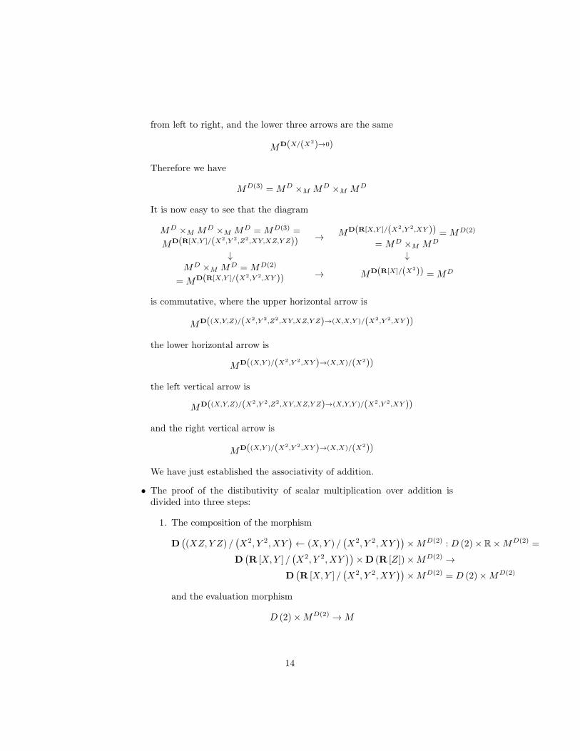
from left to right, and the lower three arrows are the same

MD(X/(X2)→0)

Therefore we have

MD(3) =MD ×M MD ×M MD

It is now easy to see that the diagram

MD ×M MD ×M MD =MD(3) =

MD(R[X,Y ]/(X2,Y 2,Z2,XY,XZ,Y Z)) →MD(R[X,Y ]/(X2,Y 2,XY )) =MD(2)

=MD ×M MD

↓ ↓

MD ×M MD =MD(2)

=MD(R[X,Y ]/(X2,Y 2,XY )) → MD(R[X]/(X2)) =MD

is commutative, where the upper horizontal arrow is

MD((X,Y,Z)/(X2,Y 2,Z2,XY,XZ,Y Z)→(X,X,Y )/(X2,Y 2,XY ))

the lower horizontal arrow is

MD((X,Y )/(X2,Y 2,XY )→(X,X)/(X2))

the left vertical arrow is

MD((X,Y,Z)/(X2,Y 2,Z2,XY,XZ,Y Z)→(X,Y,Y )/(X2,Y 2,XY ))

and the right vertical arrow is

MD((X,Y )/(X2,Y 2,XY )→(X,X)/(X2))

We have just established the associativity of addition.

• The proof of the distibutivity of scalar multiplication over addition isdivided into three steps:

1. The composition of the morphism

D((XZ, Y Z) /

(X2, Y 2, XY

)← (X,Y ) /

(X2, Y 2, XY

))×MD(2) : D (2)× R×MD(2) =

D(R [X,Y ] /

(X2, Y 2, XY

))×D (R [Z])×MD(2) →

D(R [X,Y ] /

(X2, Y 2, XY

))×MD(2) = D (2)×MD(2)

and the evaluation morphism

D (2)×MD(2) →M

14

is denoted by ψ2 : D (2)×R×MD(2) →M . Its transpose is denotedby ψ2 : R×MD(2) →MD(2). And the composition of the morphismm

D((XZ1, Y Z2) /

(X2, Y 2, XY

)← (X,Y ) /

(X2, Y 2, XY

))×MD(2) : D (2)× R× R×MD(2) =

D(R [X,Y ] /

(X2, Y 2, XY

))×D (R [Z1, Z2])×M

D(2) → D(R [X,Y ] /

(X2, Y 2, XY

))×MD(2) =

D (2)×MD(2)

and the evaluation morphism

D (2)×MD(2) →M

is denoted by χ : D (2) × R × R × MD(2) → M . Its transpose isdenoted by χ : R × R ×MD(2) → MD(2). It is easy to see that thediagram

R×MD(2)

↓ ց

R× R×MD(2) −→ MD(2)

commutes, where the vertical arrow is

D ((Z,Z)← (Z1, Z2))×MD(2) : R×MD(2) = D (R [Z])×MD(2) →

D (R [Z1, Z2])×MD(2) = R× R×MD(2)

the horizontal arrow is

χ : R× R×MD(2) →MD(2)

and the slant arrow is

ψ2 : R×MD(2) →MD(2)

It is also easy to see that the morphism χ : R×R×MD(2) →MD(2)

can be defined to be

ψ2 ×M ψ2 : R× R×MD(2) = R× R×(MD ×M MD

)=

(R×MD

)×M

(R×MD

)→MD ×M MD =MD(2)

2. Let us consider the following diagram:

D × R×MD ←− D × R×MD(2) −→ D (2)× R×MD(2)

↓ 1 ↓ 2 ↓

D ×MD ←− D ×MD(2) −→ D (2)×MD(2)

ց 3 ւ

M(4)

15

where the upper two horizontal arrows are

D × R× ϕ : D × R×MD(2) → D × R×MD

D((X,X) /

(X2

)← (X,Y ) /

(X2, Y 2, XY

))× R×MD(2) : D × R×MD(2) =

D(R [X ] /

(X2

))× R×MD(2) →

D(R [X,Y ] /

(X2, Y 2, XY

))× R×MD(2) = D (2)× R×MD(2)

from left to right, the lower two horizontal arrow are

D × ϕ : D ×MD(2) → D ×MD

D

((X,X) /

(X2

)←

(X,Y ) /(X2, Y 2, XY

))×MD(2) : D ×MD(2) = D

(R [X ] /

(X2

))×MD(2) →

D(R [X,Y ] /

(X2, Y 2, XY

))×MD(2) = D (2)×MD(2)

from left to right, the three vertical arrows are

D(XY/

(X2

)← X/

(X2

))×MD : D × R×MD =

D(R [X ] /

(X2

))×D (R [Y ])×MD → D

(R [X ] /

(X2

))×MD = D ×MD

D(XY/

(X2

)← X/

(X2

))×MD(2) : D × R×MD(2) =

D(R [X ] /

(X2

))×D (R [Y ])×MD(2) → D

(R [X ] /

(X2

))×MD(2) = D ×MD(2)

D

((XZ, Y Z) /

(X2, Y 2, XY

)

← (X,Y ) /(X2, Y 2, XY

))×MD(2) : D (2)× R×MD(2) =

D(R [X,Y ] /

(X2, Y 2, XY

))×D (R [Z])×MD(2) →

D(R [X,Y ] /

(X2, Y 2, XY

))×MD(2) = D (2)×MD(2)

from left to right, and the two slant arrows are the evaluation mor-phisms D×MD →M and D (2)×MD(2) →M . In order to establishthe commutativity of the diagram (4), we will be engaged in the com-

mutativity of the three subdiagrams 1 , 2 and 3 in order. It is

easy to see that both the diagram 1 and the digaram 2 commute.

The commutativity of the diagram 1 is a simple consequence ofthe fact that ( )× ( ) is a bifunctor, while the commutativity of the

diagram 2 follows directly from that of the following diagram

D × R −→ D (2)× R

↓ ↓

D −→ D (2)

where the two horizontal arrows are

D((X,X) /

(X2

)← (X,Y ) /

(X2, Y 2, XY

))× R : D × R =

D(R [X ] /

(X2

))× R→ D

(R [X,Y ] /

(X2, Y 2, XY

))× R = D (2)× R

D((X,X) /

(X2

)← (X,Y ) /

(X2, Y 2, XY

)): D = D

(R [X ] /

(X2

))→

D(R [X,Y ] /

(X2, Y 2, XY

))= D (2)

16

from top to bottom, and the two vertical arrows are

D(XY/

(X2

)← X/

(X2

)): D × R =

D(R [X ] /

(X2

))×D (R [Y ])→ D

(R [X ] /

(X2

))= D

D

((XZ, Y Z) /

(X2, Y 2, XY

)←

(X,Y ) /(X2, Y 2, XY

))

: D (2)× R =

D(R [X,Y ] /

(X2, Y 2, XY

))×D (R [Z])→ D

(R [X,Y ] /

(X2, Y 2, XY

))= D (2)

from left to right. The commutativity of the diagram 3 followsfrom the following commutative diagram of so-called parametrizedadjunction (cf. Theorem 3 in §IV.7 of [13]):

HomK

(D (2)×MD(2),M

)∼= HomK

(MD(2),MD(2)

)

↓ ↓

HomK

(D ×MD(2),M

)∼= HomK

(MD(2),MD

)

↑ ↑

HomK

(D ×MD,M

)∼= HomK

(MD,MD

)

(5)where the left two vertical arrows are

HomK

D

((X,X) /

(X2

)←

(X,Y ) /(X2, Y 2, XY

))

:

D = D(R [X ] /

(X2

))→

D(R [X,Y ] /

(X2, Y 2, XY

))= D (2)

×M

D(2),M

:

HomK

(D (2)×MD(2),M

)→ HomK

(D ×MD(2),M

)

HomK (D × ϕ,M) : HomK

(D ×MD,M

)→

HomK

(D ×MD(2),M

)

from top to bottom, while the right vertical arrows are

HomK

(MD(2), ϕ

): HomK

(MD(2),MD(2)

)→ HomK

(MD(2),MD

)

HomK

(ϕ,MD

): HomK

(MD,MD

)→ HomK

(MD(2),MD

)

from top to bottom. Choose

idMD(2) ∈ HomK

(MD(2),MD(2)

)

idMD ∈ HomK

(MD,MD

)

on the right of the diagram.(5). Then both yield the same morphismin HomK

(MD(2),MD

)by application of their adjacent vertical ar-

rows. The corresponding morphism of idMD(2) in HomK

(D (2)×MD(2),M

)

is no other than the evaluation morphism D (2)×MD(2) →M , and

17

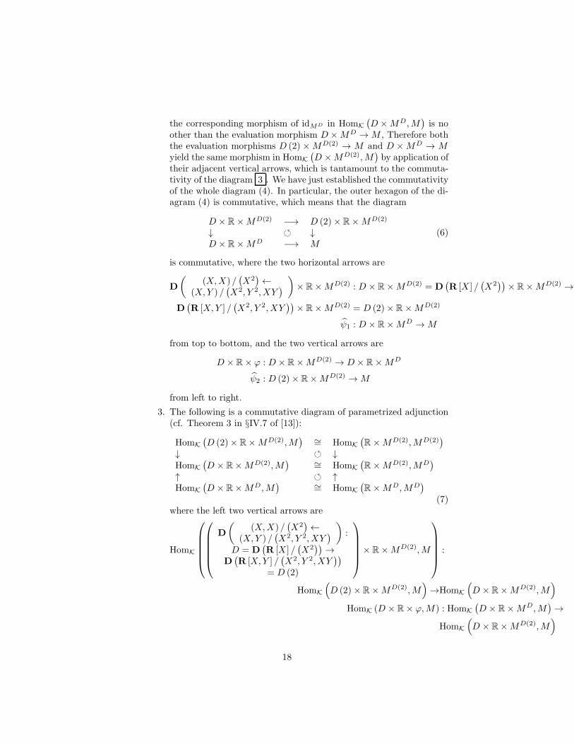
the corresponding morphism of idMD in HomK

(D ×MD,M

)is no

other than the evaluation morphism D ×MD →M , Therefore boththe evaluation morphisms D (2) ×MD(2) → M and D ×MD → Myield the same morphism in HomK

(D ×MD(2),M

)by application of

their adjacent vertical arrows, which is tantamount to the commuta-tivity of the diagram 3 . We have just established the commutativityof the whole diagram (4). In particular, the outer hexagon of the di-agram (4) is commutative, which means that the diagram

D × R×MD(2) −→ D (2)× R×MD(2)

↓ ↓

D × R×MD −→ M(6)

is commutative, where the two horizontal arrows are

D

((X,X) /

(X2

)←

(X,Y ) /(X2, Y 2, XY

))× R×MD(2) : D × R×MD(2) = D

(R [X ] /

(X2

))× R×MD(2) →

D(R [X,Y ] /

(X2, Y 2, XY

))× R×MD(2) = D (2)× R×MD(2)

ψ1 : D × R×MD →M

from top to bottom, and the two vertical arrows are

D × R× ϕ : D × R×MD(2) → D × R×MD

ψ2 : D (2)× R×MD(2) →M

from left to right.

3. The following is a commutative diagram of parametrized adjunction(cf. Theorem 3 in §IV.7 of [13]):

HomK

(D (2)× R×MD(2),M

)∼= HomK

(R×MD(2),MD(2)

)

↓ ↓

HomK

(D × R×MD(2),M

)∼= HomK

(R×MD(2),MD

)

↑ ↑

HomK

(D × R×MD,M

)∼= HomK

(R×MD,MD

)

(7)where the left two vertical arrows are

HomK

D

((X,X) /

(X2

)←

(X,Y ) /(X2, Y 2, XY

))

:

D = D(R [X ] /

(X2

))→

D(R [X,Y ] /

(X2, Y 2, XY

))

= D (2)

× R×MD(2),M

:

HomK

(D (2)× R×MD(2),M

)→HomK

(D × R×MD(2),M

)

HomK (D × R× ϕ,M) : HomK

(D × R×MD,M

)→

HomK

(D × R×MD(2),M

)

18

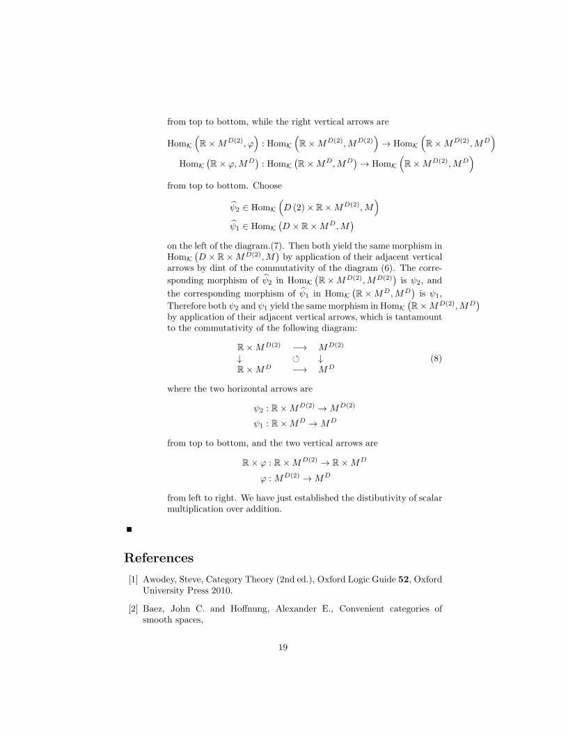
from top to bottom, while the right vertical arrows are

HomK

(R×MD(2), ϕ

): HomK

(R×MD(2),MD(2)

)→ HomK

(R×MD(2),MD

)

HomK

(R× ϕ,MD

): HomK

(R×MD,MD

)→ HomK

(R×MD(2),MD

)

from top to bottom. Choose

ψ2 ∈ HomK

(D (2)× R×MD(2),M

)

ψ1 ∈ HomK

(D × R×MD,M

)

on the left of the diagram.(7). Then both yield the same morphism inHomK

(D × R×MD(2),M

)by application of their adjacent vertical

arrows by dint of the commutativity of the diagram (6). The corre-

sponding morphism of ψ2 in HomK

(R×MD(2),MD(2)

)is ψ2, and

the corresponding morphism of ψ1 in HomK

(R×MD,MD

)is ψ1,

Therefore both ψ2 and ψ1 yield the same morphism in HomK

(R×MD(2),MD

)

by application of their adjacent vertical arrows, which is tantamountto the commutativity of the following diagram:

R×MD(2) −→ MD(2)

↓ ↓

R×MD −→ MD(8)

where the two horizontal arrows are

ψ2 : R×MD(2) →MD(2)

ψ1 : R×MD →MD

from top to bottom, and the two vertical arrows are

R× ϕ : R×MD(2) → R×MD

ϕ :MD(2) →MD

from left to right. We have just established the distibutivity of scalarmultiplication over addition.

References

[1] Awodey, Steve, Category Theory (2nd ed.), Oxford Logic Guide 52, OxfordUniversity Press 2010.

[2] Baez, John C. and Hoffnung, Alexander E., Convenient categories ofsmooth spaces,

19

[3] Bell, J. L., Toposes and Local Set Theories:an Introduction, Oxford LogicGuide 16, Oxford University Press 1988.

[4] Bertram, Wolfgang, Differential Geometry, Lie Groups and SymmetricSpaces over General Base Fields and Rings, Memoirs of the American Math-ematical Society 192, American Mathematical Society 2008

[5] Bertram, Wolfgang and Souvay, Arnaud, A general construction of Weilfunctors, Cah. Topol. Geom. Differ. Categ. 55 (2014), 267-313.

[6] Bertram, Wolfgang, Weil spaces and Weil-Lie groups, arXiv:1402.2619.

[7] Dubuc, Eduardo J., Sur les modeles de la geometrie differentiellesynthetique, Cahiers de Top. et Geom. Diff. 20 (1979), 231-279.

[8] Gabriel, Peter and Ulmer, Friedrich, Lokal prasentierbare Kategorien, Lec-ture Notes in Mathematics 221, Springer Verlag 1971.

[9] Iglesias-Zemmour, Patrick, Diffeology, Mathematical Surveys and Mono-graphs 185, American Mathematical Society 2013.

[10] Kock, Anders, Synthetic Differential Geometry (2nd edition), LondonMathematical Society Lecture Note Series 333, Cambridge University Press2006.

[11] Kolar, Ivan, Michor, Peter W. and Slovak, Jan, Natrual Operations inDifferential Geometry, Springer Verlag 1993.

[12] Lavendhomme, Rene, Basic Concepts of Synthetic Differential Geometry,Kluwer Texts in the Mathematical Sciences 13, Kluwer Academic Publish-ers 1996.

[13] Mac Lane, Saunders, Categories for the Working Mathematician, GraduateTexts in Mathematics 5, Springer Varlag 1971.

[14] Mac Lane, Saunders and Moerdijk, Ieke, Sheaves in Geometry and Logic:aFirst Introduction to Topos Theory, Universitext, Springer Verlag 1992.

[15] Moerdijk, Ieke and Reyes, Gonzalo E., Models for Smooth InfinitesimalAnalysis, Springer Verlag 1991.

[16] Nishimura, Hirokazu, Axiomatic differential geometry I-1:towards modelcategories of differential geometry, Math. Appl. (Brno) 1 (2012), 171-182.

[17] Nishimura, Hirokazu, Axiomatic differential geometry II-1:vector fields,Math. Appl. (Brno) 1 (2012), 183-195.

[18] Nishimura, Hirokazu, Axiomatic differential geometry II-2:differentialforms, Math. Appl. (Brno) 2 (2013), 43-60.

20

[19] Nishimura, Hirokazu, Axiomatic differential geometry II-3:the general Ja-cobi identity, International Journal of Pure and Applied Mathematics 83

(2013), 137-192.

[20] Nishimura, Hirokazu, Axiomatic differential geometry II-4:the Frolicher-Nijenhuis algebra, International Journal of Pure and Applied Mathematics82 (2013), 763-819.

[21] Nishimura, Hirokazu, Axiomatic differential geometry III-1:model theory I,Far East Journal of Mathematical Sciences 74 (2013), 17-26.

[22] Nishimura, Hirokazu, Axiomatic differential geometry III-2:model theoryII, Far East Journal of Mathematical Sciences 74 (2013), 139-154.

[23] Nishimura, Hirokazu, Axiomatic differential geometry III-3:the old king-dom of differential geometers, arXiv:1210.3422.

[24] Nishimura, Hirokazu, A book review of [30], Eur. Math. Soc. Newsl. 99(2016), 58-60.

[25] Nishimura, Hirokazu, A review of [30],http://hdl.handle.net/2241/00129866.

[26] Nishimura, Hirokazu, Weil diffeology II:homotopical differential geometry,in preparation.

[27] Nishimura, Hirokazu, Weil diffeology III:higher differential geometry, inpreparation.

[28] Nishimura, Hirokazu, Weil diffeology IV:supergeometry, in preparation.

[29] Nishimura, Hirokazu, Weil diffeology V:braided differential geometry, inpreparation.

[30] Paugam, Frederic, Towards the Mathematics of Quantum Field Theory,Springer Verlag 2014.

[31] Souriau, Jean-Marie, Groupes differentiels, Lecture Notes in Mathematics(1980), Springer-Verlag.

[32] Stacey, Andrew, Comparative smootheology, Theory and Applications ofCategories, 25 (2011), 64-117.

[33] Steenrod, Norman, A convenient category of topological spaces, MichiganMath. Journal 14 (1967), 133-152.

[34] Weil, Andre, Theorie des points proches sur les varietes differentiables, inColloq. Top. et Geom. Diff., Strassbourg, 1953.

21