Applied Mathematics, 2017, 8, 645-654 http://www.scirp.org/journal/am

ISSN Online: 2152-7393 ISSN Print: 2152-7385

Weighted Least-Squares for a Nearly Perfect Min-Max Fit

Isaac Fried, Ye Feng

Department of Mathematics, Boston University, Boston, MA, USA

Abstract In this note, we experimentally demonstrate, on a variety of analytic and nonanalytic functions, the novel observation that if the least squares poly-nomial approximation is repeated as weight in a second, now weighted, least squares approximation, then this new, second, approximation is nearly perfect in the uniform sense, barely needing any further, say, Remez correction. Keywords Least Squares-Approximation of Functions, Weighted Approximations, Nearly Perfect Uniform Fits

1. Introduction

Finding the min-max, or best L∞ , polynomial approximation to a function, in some standard interval, is of the greatest interest in numerical analysis [1] [2]. For a polynomial function the least error distribution is a Chebyshev polynomial [3] [4] [5].

The usual procedure [6] [7] to find the best L∞ approximation to a general function is to start with a good approximation, say in the 2L sense, easily ob-tained by the minimization of a quadratic functional for the coefficients, then iteratively improving this initial approximation by a Remez-like correction pro-cedure [8] [9] that strives to produce an error distribution that oscillates with a constant amplitude in the interval of interest.

In this note, we bring ample and varied computational evidence in support of the novel, worthy of notice, empirical numerical observation that taking the er-ror distribution of a least squares, 2L , best polynomial fit to a function, squared, as weight in a second, weighted, least squares approximation, results in an error distribution that is remarkably close to the best L∞ , or uniform, approximation.

How to cite this paper: Fried, I. and Feng, Y. (2017) Weighted Least-Squares for a Nearly Perfect Min-Max Fit. Applied Ma-thematics, 8, 645-654. https://doi.org/10.4236/am.2017.85051 Received: February 28, 2017 Accepted: May 19, 2017 Published: May 22, 2017 Copyright © 2017 by authors and Scientific Research Publishing Inc. This work is licensed under the Creative Commons Attribution International License (CC BY 4.0). http://creativecommons.org/licenses/by/4.0/

Open Access

DOI: 10.4236/am.2017.85051 May 22, 2017

I. Fried, Y. Feng

2. Fixing Ideas; The Best Quadratic in [−1, 1]

The monic Chebyshev polynomial

( ) 22

1 , 1 12

T x x x= − − ≤ ≤ (1)

is the solution of the min-max problem

( ) ( ) 2min max , , 1 1.a x

e x e x x a x= − − ≤ ≤ (2)

This min-max solution, the least function in the L∞ sense, is a polynomial that has two distinct roots, and oscillates with a constant amplitude in

1 1,x− ≤ ≤ ( ) ( ) ( )1 0 1 .e e e− = − = Indeed, say 21 0 1e x a a x= + + is such a po-

lynomial, and 22 0 1e x p p x= + + is another quadratic polynomial, then 1 2e e≤

in the interval, for otherwise 1e and 2e would intersect at two points, which is absurd; 2 2

0 1 0 1x a a x x p p x+ + = + + is either an identity, or has but the one solution ( ) ( )0 0 1 1x p a p a= − − − .

Thus, the monic Chebyshev polynomial of degree n is the least, uniform, or pointwise, error distribution in approximating nx by a polynomial of degree

1n − . To obtain a least squares, a best 2L , approximation to ( )2T x we first mi-

nimize ( )I a

( ) ( ) ( ) ( )21 12 21 1

d , d 0I a x a x I a x a x− −

′= − = − =∫ ∫ (3)

to have the value 1 3 0.3333a = = . Minimizing next ( )I p , under the weight ( )22 , 1 3x a a− =

( ) ( ) ( ) ( ) ( ) ( )2 2 21 12 2 2 21 1

1 3 d , 1 3 d 0I p x x p x I p x p x x− −

′= − − = − − =∫ ∫ (4)

now with respect to p, we obtain 11 21 0.5238p = = , which is surprisingly much closer to the optimal value of one half.

We may replace the difficult L∞ measure by the computationally easier mL measure with an even 1m . Let a0 be a good approximation, and 1 0a a δ= + be an improved one. Minimization cum linearization produces the equation

( ) ( ) 11 12 20 01 1

d d 0n n

x a x n x a xδ−

− −− − − =∫ ∫ (5)

where 1n is odd. Starting with 0 11 21 0.5238a = = , we obtain from the above equation, for

17n = , the value 1 0.495a = , as compared with the optimal 0.5a = .

3. Optimal Cubic in [−1, 1]

Seeking to reproduce the optimal monic Chebyshev polynomial of degree three

( ) 33

3 , 1 14

T x x x x= − − ≤ ≤ (6)

we start by minimizing ( )1I a

( ) ( ) ( ) ( )21 13 31 1 1 11 1

d , d 0I a x a x x I a x x a x x− −

′= − = − =∫ ∫ (7)

646

I. Fried, Y. Feng

and have 1 3 5 0.6a = = . Then we return to minimize the weighted ( )1I p with respect to 1p

( ) ( ) ( )( ) ( ) ( )

2 21 3 31 1 11

21 3 31 1 11

d ,

d 0

I p x a x x p x x

I p x x a x x p x x

−

−

= − −

′ = − − =

∫

∫ (8)

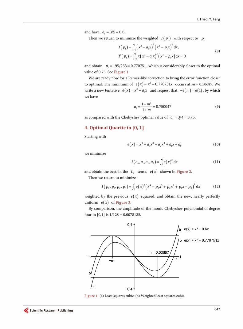
and obtain 1 195 253 0.770751p = = , which is considerably closer to the optimal value of 0.75. See Figure 1.

We are ready now for a Remez-like correction to bring the error function closer to optimal. The minimum of ( ) 3 0.770751e x x x= − occurs at m = 0.50687. We write a new tentative ( ) 3

1e x x a x= − and request that ( ) ( )1e m e− = , by which we have

3

11 0.7500471

mam

+= =

+ (9)

as compared with the Chebyshev optimal value of 1 3 4 0.75a = = .

4. Optimal Quartic in [0, 1]

Starting with

( ) 4 3 23 2 1 0e x x a x a x a x a= + + + + (10)

we minimize

( ) ( )1 20 1 2 3 0, , , dI a a a a e x x= ∫ (11)

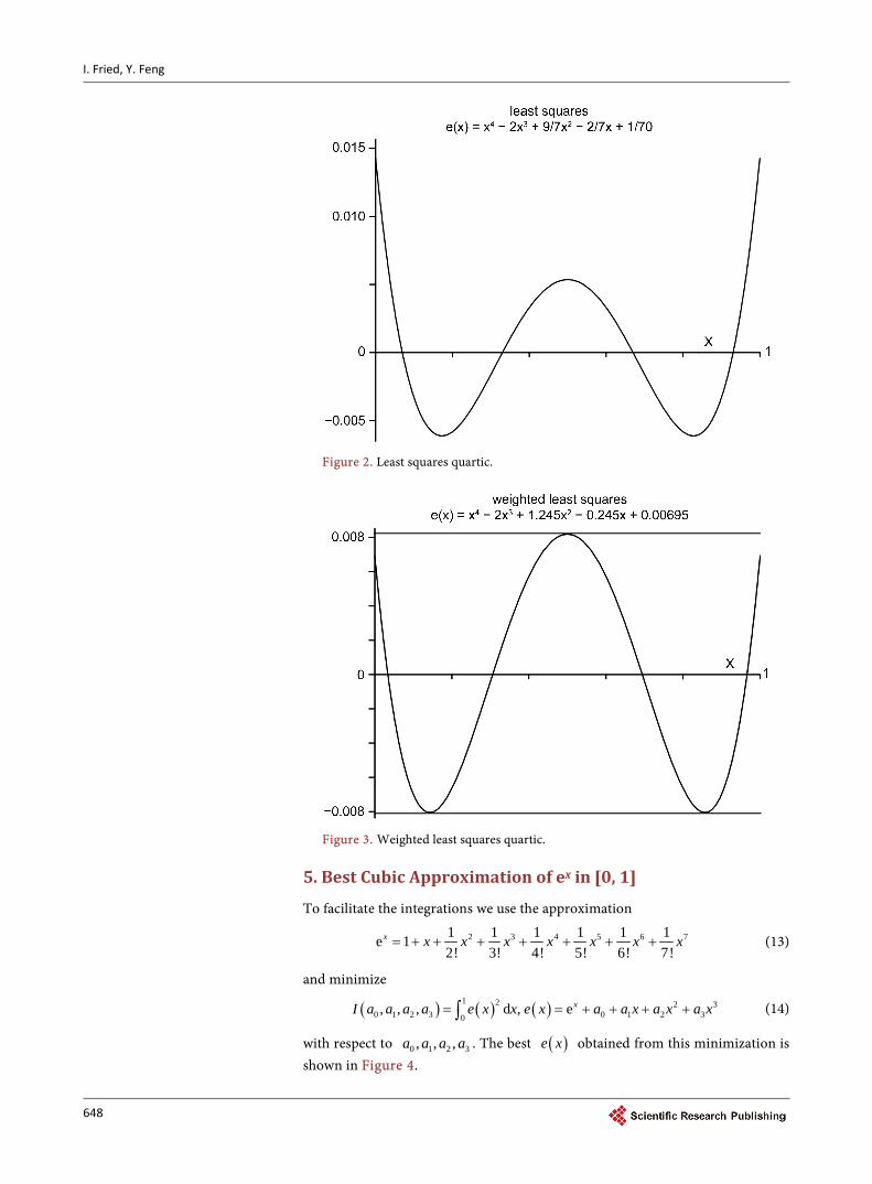
and obtain the best, in the 2L sense, ( )e x shown in Figure 2. Then we return to minimize

( ) ( ) ( )21 2 4 3 20 1 2 3 3 2 1 00, , , dI p p p p e x x p x p x p x p x= + + + +∫ (12)

weighted by the previous ( )e x squared, and obtain the new, nearly perfectly uniform ( )e x of Figure 3.

By comparison, the amplitude of the monic Chebyshev polynomial of degree four in [0,1] is 1/128 = 0.0078125.

Figure 1. (a) Least squares cubic. (b) Weighted least squares cubic.

647

I. Fried, Y. Feng

Figure 2. Least squares quartic.

Figure 3. Weighted least squares quartic.

5. Best Cubic Approximation of ex in [0, 1]

To facilitate the integrations we use the approximation

2 3 4 5 6 71 1 1 1 1 1e 12! 3! 4! 5! 6! 7!

x x x x x x x x= + + + + + + + (13)

and minimize

( ) ( ) ( )1 2 2 30 1 2 3 0 1 2 30, , , d , exI a a a a e x x e x a a x a x a x= = + + + +∫ (14)

with respect to 0 1 2 3, , ,a a a a . The best ( )e x obtained from this minimization is shown in Figure 4.

648

I. Fried, Y. Feng

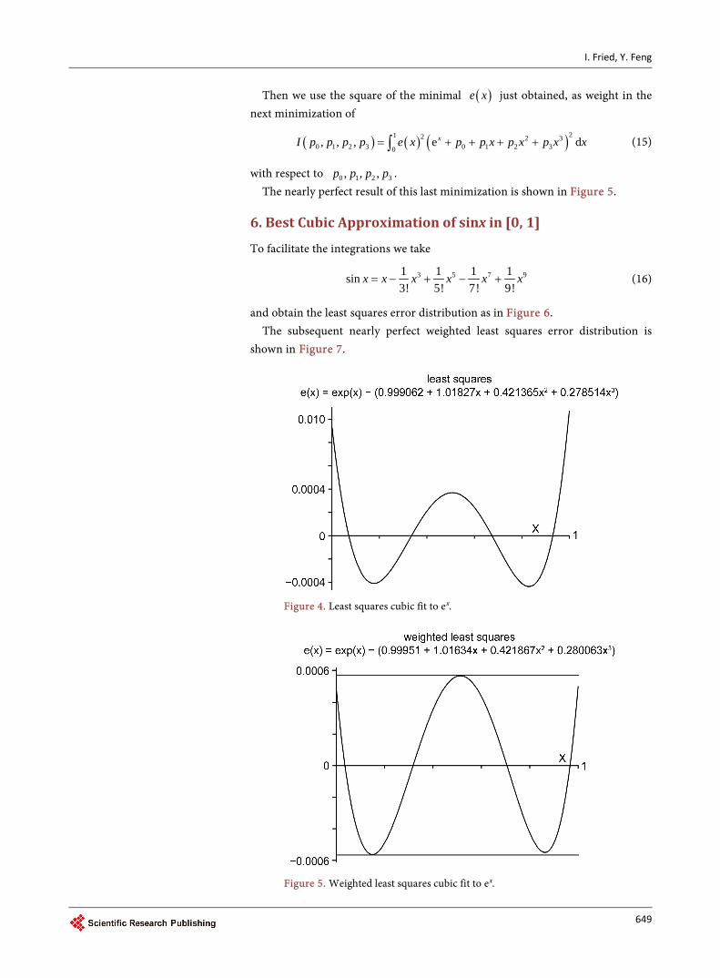
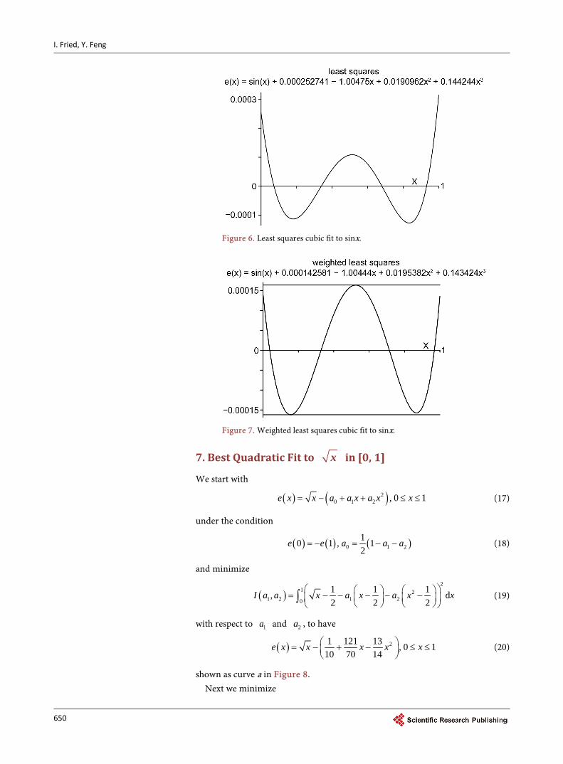
Then we use the square of the minimal ( )e x just obtained, as weight in the next minimization of

( ) ( ) ( )21 2 2 30 1 2 3 0 1 2 30, , , e dxI p p p p e x p p x p x p x x= + + + +∫ (15)

with respect to 0 1 2 3, , ,p p p p . The nearly perfect result of this last minimization is shown in Figure 5.

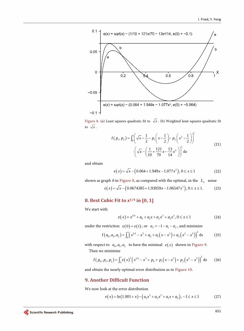
6. Best Cubic Approximation of sinx in [0, 1]

To facilitate the integrations we take

3 5 7 91 1 1 1sin3! 5! 7! 9!

x x x x x x= − + − + (16)

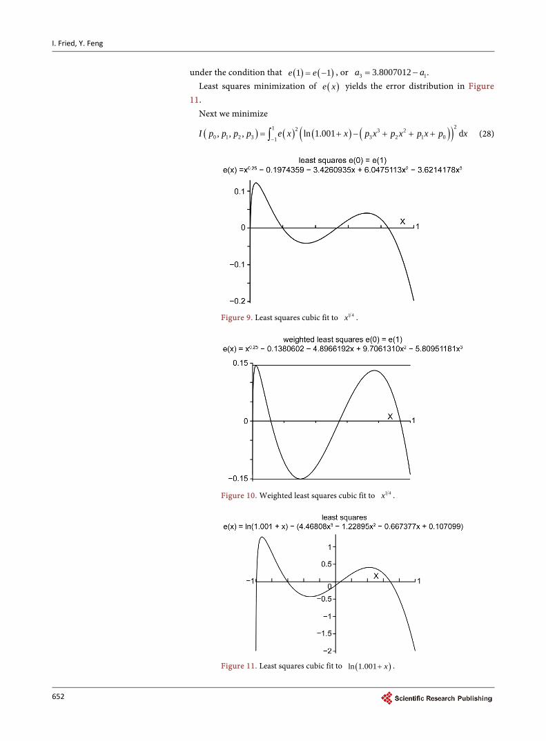
and obtain the least squares error distribution as in Figure 6. The subsequent nearly perfect weighted least squares error distribution is

shown in Figure 7.

Figure 4. Least squares cubic fit to ex.

Figure 5. Weighted least squares cubic fit to ex.

649

I. Fried, Y. Feng

Figure 6. Least squares cubic fit to sinx.

Figure 7. Weighted least squares cubic fit to sinx.

7. Best Quadratic Fit to x in [0, 1]

We start with

( ) ( )20 1 2 , 0 1e x x a a x a x x= − + + ≤ ≤ (17)

under the condition

( ) ( ) ( )0 1 210 1 , 12

e e a a a= − = − − (18)

and minimize

( )2

1 21 2 1 20

1 1 1, d2 2 2

I a a x a x a x x = − − − − −

∫ (19)

with respect to 1a and 2a , to have

( ) 21 121 13 , 0 110 70 14

e x x x x x = − + − ≤ ≤

(20)

shown as curve a in Figure 8. Next we minimize

650

I. Fried, Y. Feng

Figure 8. (a) Least squares quadratic fit to x . (b) Weighted least squares quadratic fit to x .

( )2

1 21 2 1 20

22

1 1 1,2 2 2

1 121 13 d10 70 14

I p p x p x p x

x x x x

= − − − − −

⋅ − + −

∫ (21)

and obtain

( ) ( )20.064 1.949 1.077 , 0 1e x x x x x= − + − ≤ ≤ (22)

shown as graph b in Figure 8, as compared with the optimal, in the L∞ sense

( ) ( )20.0674385 1.93059 1.06547 , 0 1.e x x x x x= − + − ≤ ≤ (23)

8. Best Cubic Fit to x1/4 in [0, 1]

We start with

( ) 1 4 2 30 1 2 3 , 0 1e x x a a x a x a x x= + + + + ≤ ≤ (24)

under the restriction ( ) ( )0 1e e= , or 3 1 21a a a= − − − , and minimize

( ) ( ) ( )( )21 1 4 3 3 2 30 1 2 0 1 20, , dI a a a x x a a x x a x x x= − + + − + −∫ (25)

with respect to 0 1 2, ,a a a to have the minimal ( )e x shown in Figure 9. Then we minimize

( ) ( ) ( ) ( )( )21 2 1 4 3 3 2 30 1 2 0 1 20, , dI p p p e x x x p p x x p x x x= − + + − + −∫ (26)

and obtain the nearly optimal error distribution as in Figure 10.

9. Another Difficult Function

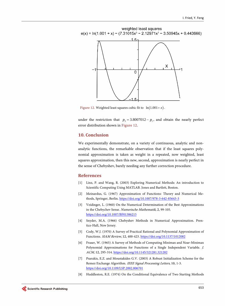
We now look at the error distribution

( ) ( ) ( )3 23 2 1 0ln 1.001 , 1 1e x x a x a x a x a x= + − + + + − ≤ ≤ (27)

651

I. Fried, Y. Feng

under the condition that ( ) ( )1 1e e= − , or 3 13.8007012 .a a= − Least squares minimization of ( )e x yields the error distribution in Figure

11. Next we minimize

( ) ( ) ( ) ( )( )21 2 3 20 1 2 3 3 2 1 01, , , ln 1.001 dI p p p p e x x p x p x p x p x

−= + − + + +∫ (28)

Figure 9. Least squares cubic fit to 1 4x .

Figure 10. Weighted least squares cubic fit to 1 4x .

Figure 11. Least squares cubic fit to ( )ln 1.001 x+ .

652

I. Fried, Y. Feng

Figure 12. Weighted least squares cubic fit to ( )ln 1.001 x+ .

under the restriction that 3 13.8007012p p= − , and obtain the nearly perfect error distribution shown in Figure 12.

10. Conclusion

We experimentally demonstrate, on a variety of continuous, analytic and non-analytic functions, the remarkable observation that if the least squares poly-nomial approximation is taken as weight in a repeated, now weighted, least squares approximation, then this new, second, approximation is nearly perfect in the sense of Chebyshev, barely needing any further correction procedure.

References [1] Linz, P. and Wang, R. (2003) Exploring Numerical Methods: An introduction to

Scientific Computing Using MATLAB. Jones and Bartlett, Boston.

[2] Meinardus, G. (1967) Approximation of Functions: Theory and Numerical Me-thods, Springer, Berlin. https://doi.org/10.1007/978-3-642-85643-3

[3] Veidinger, L. (1960) On the Numerical Determination of the Best Approximations in the Chebychev Sense. Numerische Mathematik, 2, 99-105. https://doi.org/10.1007/BF01386215

[4] Snyder, M.A. (1966) Chebyshev Methods in Numerical Approximation. Pren-tice-Hall, New Jersey.

[5] Cody, W.J. (1970) A Survey of Practical Rational and Polynomial Approximation of Functions. SIAM Review, 12, 400-423. https://doi.org/10.1137/1012082

[6] Fraser, W. (1965) A Survey of Methods of Computing Minimax and Near-Minimax Polynomial Approximations for Functions of a Single Independent Variable. J. ACM, 12, 295-314. https://doi.org/10.1145/321281.321282

[7] Psarakis, E.Z. and Moustakides G.V. (2003) A Robust Initialization Scheme for the Remez Exchange Algorithm. IEEE Signal Processing Letters, 10, 1-3. https://doi.org/10.1109/LSP.2002.806701

[8] Huddleston, R.E. (1974) On the Conditional Equivalence of Two Starting Methods

653

I. Fried, Y. Feng

for the Second Algorithm of Remez. Mathematics of Computation, 28, 569-572. https://doi.org/10.1090/S0025-5718-1974-0341804-6

[9] Pachon, R. and Trefethen, L.N. (2009) Barycentric-Remez Algorithms for Best Po-lynomial Approximation in the chebfun System. BIT Numerical Mathematics, 49, 721-741. https://doi.org/10.1007/s10543-009-0240-1

Submit or recommend next manuscript to SCIRP and we will provide best service for you:

Accepting pre-submission inquiries through Email, Facebook, LinkedIn, Twitter, etc. A wide selection of journals (inclusive of 9 subjects, more than 200 journals) Providing 24-hour high-quality service User-friendly online submission system Fair and swift peer-review system Efficient typesetting and proofreading procedure Display of the result of downloads and visits, as well as the number of cited articles Maximum dissemination of your research work

Submit your manuscript at: http://papersubmission.scirp.org/ Or contact am@scirp.org

654