Embed Size (px)
Citation preview
Weighted Hurwitz numbers and topological recursion
A. Alexandrov1,2,3∗, G. Chapuy4†, B. Eynard2,5‡ and J. Harnad2,6§
1Center for Geometry and Physics, Institute for Basic Science (IBS), Pohang 37673, Korea2Centre de recherches mathematiques, Universite de MontrealC. P. 6128, succ. centre ville, Montreal, QC H3C 3J7 Canada
3ITEP, Bolshaya Cheremushkinskaya 25, 117218 Moscow, Russia4CNRS, IRIF UMR 8243, Universite Paris Diderot
Paris 7, Case 7014 75205 Paris Cedex 13 France5Institut de Physique Theorique, CEA, IPhT,
F-91191 Gif-sur-Yvette, FranceCNRS URA 2306, F-91191 Gif-sur-Yvette, France
6Department of Mathematics and Statistics, Concordia University
1455 de Maisonneuve Blvd. W. Montreal, QC H3G 1M8 Canada
May 28, 2019
Abstract
The KP and 2D Toda τ -functions of hypergeometric type that serve as generatingfunctions for weighted single and double Hurwitz numbers are related to the topologicalrecursion programme. A graphical representation of such weighted Hurwitz numbersis given in terms of weighted constellations. The associated classical and quantumspectral curves are derived, and these are interpreted combinatorially in terms of thegraphical model. The pair correlators are given a finite Christoffel-Darboux represen-tation and determinantal expressions are obtained for the multipair correlators. Thegenus expansion of the multicurrent correlators is shown to provide generating seriesfor weighted Hurwitz numbers of fixed ramification profile lengths. The WKB series forthe Baker function is derived and used to deduce the loop equations and the topologicalrecursion relations.
∗e-mail: [email protected]†e-mail: [email protected]‡e-mail: [email protected]§e-mail: [email protected]
1
arX
iv:1
806.
0973
8v5
[m
ath-
ph]
25
May
201
9
Contents
1 Introduction and main result 3
1.1 Introduction . . . . . . . . . . . . . . . . . . . . . . . . . . . . . . . . . . . . 3
1.2 Main result . . . . . . . . . . . . . . . . . . . . . . . . . . . . . . . . . . . . 6
1.3 Outline . . . . . . . . . . . . . . . . . . . . . . . . . . . . . . . . . . . . . . . 7
2 Weighted Hurwitz numbers and τ-functions as generating functions 8
2.1 Weighted Hurwitz numbers . . . . . . . . . . . . . . . . . . . . . . . . . . . 9
2.2 The τ -functions τ (G,β,γ)(t, s) . . . . . . . . . . . . . . . . . . . . . . . . . . . 11
2.3 Convolution action and dressing: adapted bases . . . . . . . . . . . . . . . . 13
3 Constellations 14
3.1 Constellations and branched covers . . . . . . . . . . . . . . . . . . . . . . . 14
3.2 Weighted constellations . . . . . . . . . . . . . . . . . . . . . . . . . . . . . . 17
3.3 Reconstructing the τ -function . . . . . . . . . . . . . . . . . . . . . . . . . . 18
3.4 Direct correspondence between constellations and coverings . . . . . . . . . . 18
4 Fermionic and bosonic functions 20
4.1 Fermionic functions . . . . . . . . . . . . . . . . . . . . . . . . . . . . . . . . 21
4.2 Bosonic functions . . . . . . . . . . . . . . . . . . . . . . . . . . . . . . . . . 22
4.3 From bosons to fermions . . . . . . . . . . . . . . . . . . . . . . . . . . . . . 25
4.4 From fermions to bosons . . . . . . . . . . . . . . . . . . . . . . . . . . . . . 26
4.5 Expansion of K(x, x′) for the case τ (G,β,γ)(t, β−1s) . . . . . . . . . . . . . . . 27
5 Adapted bases, recursion operators and the Christoffel-Darboux relation 28
5.1 Recursion operators and adapted basis . . . . . . . . . . . . . . . . . . . . . 28
5.2 The Christoffel-Darboux relation . . . . . . . . . . . . . . . . . . . . . . . . 31
6 The quantum spectral curve and first order linear differential systems 32
6.1 The quantum spectral curve . . . . . . . . . . . . . . . . . . . . . . . . . . . 32
6.2 The infinite differential system . . . . . . . . . . . . . . . . . . . . . . . . . . 33
6.3 Folding: finite-dimensional linear differential system . . . . . . . . . . . . . . 34
6.4 Adjoint differential system . . . . . . . . . . . . . . . . . . . . . . . . . . . . 35
6.5 The current correlators Wn . . . . . . . . . . . . . . . . . . . . . . . . . . . . 36
7 Classical spectral curve and local expansions 37
7.1 The classical spectral curve . . . . . . . . . . . . . . . . . . . . . . . . . . . 37
7.2 Some geometry . . . . . . . . . . . . . . . . . . . . . . . . . . . . . . . . . . 37
7.2.1 Branch points and ramification points . . . . . . . . . . . . . . . . . . 37
2
7.2.2 Labelling the roots . . . . . . . . . . . . . . . . . . . . . . . . . . . . 39
7.2.3 Galois involutions . . . . . . . . . . . . . . . . . . . . . . . . . . . . . 40
8 WKB β-expansions and their poles 40
8.1 WKB β-expansion of Ψ+k , Ψ−k and K . . . . . . . . . . . . . . . . . . . . . . 40
8.2 Definition and poles of ωg,n . . . . . . . . . . . . . . . . . . . . . . . . . . . . 45
9 Fundamental system and loop equations 48
9.1 The fundamental system . . . . . . . . . . . . . . . . . . . . . . . . . . . . . 48
9.2 Loop equations . . . . . . . . . . . . . . . . . . . . . . . . . . . . . . . . . . 50
10 Topological recursion 51
10.1 Topological recursion for the ωg,n’s . . . . . . . . . . . . . . . . . . . . . . . 52
10.2 Applications, examples, and further comments. . . . . . . . . . . . . . . . . . 52
A Appendices: Proofs 54
A.1 Section 4 . . . . . . . . . . . . . . . . . . . . . . . . . . . . . . . . . . . . . . 54
A.2 Section 5 . . . . . . . . . . . . . . . . . . . . . . . . . . . . . . . . . . . . . . 55
A.3 Section 6 . . . . . . . . . . . . . . . . . . . . . . . . . . . . . . . . . . . . . . 57
A.4 Section 7 . . . . . . . . . . . . . . . . . . . . . . . . . . . . . . . . . . . . . . 61
A.5 Section 8 . . . . . . . . . . . . . . . . . . . . . . . . . . . . . . . . . . . . . . 61
A.6 Section 9 . . . . . . . . . . . . . . . . . . . . . . . . . . . . . . . . . . . . . . 65
A.7 Section 10 . . . . . . . . . . . . . . . . . . . . . . . . . . . . . . . . . . . . . 68
1 Introduction and main result
1.1 Introduction
In their original geometric sense, Hurwitz numbers enumerate N -fold ramified coverings of
the Riemann sphere with given ramification types at the branch points. They can also
be interpreted combinatorially as enumerating factorizations of the identity element of the
symmetric group SN into a product of elements belonging to given conjugacy classes. They
were first introduced and studied by Hurwitz [46,47] and subsequently related to the structure
and characters of the symmetric group by Frobenius [32, 33].
Many variants and refinements have been been studied in recent years [1,2,4,5,8–10,15,
19,35,36,38–41,44,52,56,58,60–62,64,65,68,81], culminating in the introduction of weighted
Hurwitz numbers [38, 39, 41, 44], which are weighted sums of Hurwitz numbers depending
on a finite or infinite number of weighting parameters. All recently studied variants are
special cases of these, or suitably defined limits. Combinatorially, the weighted enumeration
of branched coverings is equivalent to the weighted enumeration of families of embedded
3
graphs such as maps, dessins d’enfants, or more generally, constellations [54]. There has
also been important progress in relating Hurwitz numbers to other classes of enumerative
geometric invariants [5,19,23,30,37,51,61,64,65,68] and matrix models [1,2,4,9,10,15,19,
22,57,60,64,65].
A key development was the identification by Pandharipande [68] and Okounkov [61] that
certain special τ -functions for integrable hierarchies of the KP and 2D Toda type may serve as
generating functions for simple (single and double) Hurwitz numbers (i.e., those for which all
branch points, with the possible exception of one, or two, have simple ramification profiles).
It was shown subsequently [9,10,38,39,41,44] that all weighted (single and double) Hurwitz
numbers have KP or 2D Toda τ -functions of the special hypergeometric type [63, 66, 67] as
generating functions.
An alternative approach, particularly useful for studying genus dependence and recursive
relations between the invariants involved [37], consists of using multicurrent correlators as
generating functions for weighted Hurwitz numbers having a fixed ramification profile length
n. These may be defined in a number of equivalent ways: either as the coefficients in
multivariable Taylor series expansions of the τ -function about suitably defined n-parameter
families of evaluation points, in terms of pair correlators, or as fermionic expectation values
of products of current operators evaluated at n points [7].
A very efficient way of computing Hurwitz numbers, which provides strong results about
their structure, follows from the method of Topological Recursion (TR), introduced by Ey-
nard and Orantin in [27]. This approach, originally inspired by results arising naturally in
random matrix theory [24], has been shown applicable to many enumerative geometry prob-
lems, such as the counting of maps [25] or computation of Gromov-Witten invariants [18].
It has received a great deal of attention in recent years and found to have many far-reaching
implications. The fact that simple Hurwitz numbers satisfy the TR relations was conjec-
tured by Bouchard and Marino [19], and proved in [15,26]. This provides an algorithm that
allows them to be computed by recursion in the Euler characteristic, starting from initial
data corresponding to the so-called “disk” and “cylinder” case (which in the notation of the
present paper correspond to genus g = 0 and n = 1, 2, respectively).
The basic recursive algorithm is the same in all these problems, the only difference being
the so-called spectral curve that corresponds to the initial data. In the case of weighted
Hurwitz numbers, it implies connections between their structural properties and relates them
to other areas of enumerative geometry. In particular, it implies the existence of formulae
of ELSV type [23, 30], relating Hodge invariants, ψ-classes and Hurwitz numbers. It is
interesting to note that, although TR and its consequences are universal (only the spectral
curve changes), the detailed proofs of its validity in the various models are often distinct,
model-dependent and, to some extent, ad hoc.
In the present work we prove, under certain technical assumptions, that weighted Hurwitz
numbers satisfy the TR relations. For brevity and simplicity, we assume that the weight
4
generating function G(z), and the exponential factor S(z) determining the second set of KP
flows in the 2D Toda model are polynomials, leaving the extension of these results to more
general cases to further work. For combinatorialists, we emphasize that the main result may
be interpreted equivalently as applying to suitably weighted enumeration of constellations,
as explained below.
The main conclusions were previously announced in the overview paper [6] and are sum-
marized in Subsections 1.2 and 1.3. They rely in part on results proved in [6] and in the
companion paper [7] on fermionic representations. In certain cases, new proofs are provided
that have a different form from those in [7].
Remark 1.1. The fact that weighted Hurwitz numbers satisfy the TR relations deeply in-
volves their integrable structure and requires a rather intricate sequence of preparatory results,
each of which has its own independent interest. Such results have always been a challenge
to prove, with characteristically different difficulties for every enumerative geometry problem
considered. This can perhaps be understood, considering that TR is interpretable as a form
of mirror symmetry [18].
We proceed through the following sequence of preparatory steps.
1. The generating functions for weighted Hurwitz numbers are related to certain integral
kernels (pair correlators, or 2-point functions) and their 2n-point generalizations. These
are shown to satisfy determinantal formulae that follow from their expression in terms
of τ -functions, which themselves are given by Fredholm determinants.
2. The integral kernels are shown to have a Christoffel-Darboux-like form (sometimes called
integrable kernels [42, 48, 76]), with numerators consisting of a finite sum over bilinear
combinations of solutions of a linear differential system with rational coefficients, and a
Cauchy-type denominator.
3. This property, together with the expansion of the generating functions and Baker func-
tions in a small parameter β appearing in the definition of the τ -function, is used to
derive a WKB-like expansion, with powers corresponding to the Euler characteristic;
hence, a topological expansion. Moreover, using the differential system, the generating
functions are shown to have poles only at the branch points of the spectral curve, a
non-trivial property.
4. The differential system is also used to prove that generating functions for weighted
Hurwitz numbers satisfy a set of consistency conditions, the loop equations.
5. These equations are used, together with the fact that the generating functions are an-
alytic away from the branch points, to prove the Topological Recursion (TR) relations,
along lines developed in [27].
5
1.2 Main result
The main result of this work is that the coefficients Wg,n(x1, . . . , xn) of multicurrent correla-
tors in a genus expansion serve as generating functions for weighted double Hurwitz numbers
HdG(µ, ν), with weights determined by weight generating function G(z), and satisfy the topo-
logical recursion (TR) relations. The complete statement of this fact requires a number of
preparatory definitions and results; it is given in Theorem 10.1, Section 10. For genus g ≥ 0
and n ≥ 1 points in the correlator, let
Wg,n(x1, . . . , xn) ≡ WGg,n(s; γ;x1, . . . , xn) (1.1)
denote the generating function (see eqs. (4.20) - (4.26)) for weighted double Hurwitz numbers
HdG(µ, ν) associated to the (g, n) step of the recursion. The Wg,n’s are identified in Section 4
as coefficients in the β-expansion of the multicurrent correlation function Wn(x1, . . . , xn)
associated to the underlying 2D-Toda τ -function τ (G,β,γ)(t, s) of hypergeometric type. The β
dependence follows from evaluations of the function G(z) that generate the weighting factor
WG(µ(1), . . . , µ(k)) in the definition (2.17) of HdG(µ, ν). The variables xii=1,...,n are viewed
as evaluations of the spectral parameter, and the second set of 2D-Toda flow parameters,
denoted s = (s1, s2, . . . ), serve as bookkeeping parameters that record the part lengths in the
“second partition” ν of the double Hurwitz numbers HdG(µ, ν). Powers of β in the expansion
of Wn(x1, . . . , xn) keep track of the genus of the covering curve, and β also serves as the
small parameter in the WKB expansion of the wave function (or Baker function). Powers
of an auxiliary parameter γ in the multiple parameter expansion keep track of the degree of
the covering.
The following is an abbreviated version of the main result. (See Section 10, Theorem 10.1,
for a more precise statement.)
Theorem 1.1. Choosing both G(z) and S(z) =∑
k≥1 kskzk as polynomials in z, the rami-
fication points of the algebraic plane curve (the spectral curve)
xy = S (γxG(xy)) , (1.2)
with rational parametrization:
X(z) :=z
γG(S(z)), Y (z) :=
S(z)
zγG(S(z)), (1.3)
under the projection map (x, y)→ x are given by the zeros of the polynomial
G(S(z))− zG′(S(z))S ′(z), (1.4)
which are assumed to all be simple. The (multicurrent) correlators Wg,n(x1, . . . , xn) then
satisfy the Eynard-Orantin topological recursion relations given by eqs. (10.2 - 10.3), with
spectral curve (1.2), (1.3).
6
Remark 1.2. We restrict ourselves to the case of simple branch points and polynomial G(z)
and S(z). The first restriction is mainly for the sake of simplicity; as will appear, the proofs
are already quite technical. For higher ramification types, an extended version of topological
recursion is expected to hold [17]. The second restriction is more essential, and we do not
expect that our results can be immedeately extended to the most generic non-polynomial case.
Although it is natural to expect that many of the techniques applied here can be adapted when
these restrictions are removed, we do not pursue this here. (See the remarks at the end of
Section 10.2.)
Remark 1.3. Probably the best-known example of weighted Hurwitz numbers for polynomial
weight generating function G(z) is given by strictly monotone Hurwitz numbers, or dessins
d’enfants, or hypermaps corresponding to ramified covers of P1 with at most three branch
points, for which
G(z) = 1 + z. (1.5)
The orbifold case corresponds to the monomial S(z) = zr. The quantum curve for this
case was earlier obtained in [21] using combinatorics of hypermaps and in [22] using the
loop equations for hypermaps. Topological recursion was discussed in [22, 52]. For the more
general case of double strictly monotone Hurwitz numbers, relevant to this paper, the quantum
spectral curve equation was derived in [8].
Remark 1.4. To help readers with a background mainly in combinatorics in understanding
the meaning of this theorem, we note that the function Wg,n(x1, . . . ,n ) is just the exponential
generating function, in the parameter γ, of double weighted Hurwitz numbers of genus g,
with weighting function G(z). The first partition has n parts whose lengths are marked by
the variables x1, . . . , xn, and for each i ≥ 1 the variable si marks the parts of length i in the
second partition. It can also be thought of as a generating function of constellations of genus
g with n vertices of a given colour, as explained below. Topological recursion gives an explicit
way to compute these functions recursively in closed form, and provides much information
about their structure.
1.3 Outline
In Section 2 weighted Hurwitz numbers are defined and the parametric family of 2D Toda
τ -functions that serve as generating functions for these is introduced. Section 3 presents a
classical graphical model for weighted enumeration of branched covers consisting of weighted
constellations. Section 4 introduces several families of functions, identified either as fermionic
or bosonic, associated to the τ -function and gives the relations between these; namely: 1)
the multicurrent correlators Wn and their coefficients Wg,n in the genus expansion that
appears in our main result; 2) a pair of dual bases Ψ±k that extend the Baker function and
its dual and are adapted to a basis of the infinite Grassmannian element that determines
7
the τ -function, and 3) the pair correlation kernel K and its n-pair generalization Kn. In
Section 5 an operator formalism adapted to these quantities is developed and used to derive
a bilinear formula of Christoffel-Darboux type for K. In Section 6 infinite and finite linear
differential systems satisfied by the Ψ±k ’s, are studied, together with recursion relations that
allow the infinite to be mapped onto the finite ones by “folding”. In particular, this leads to
the quantum spectral curve equation. Section 7 concerns basic geometric properties of the
classical spectral curve and its branch points, a necessary step in establishing the topological
recursion relations. In Section 8 a key technical result about the rational structure and poles
of the multidifferentials ωg,n corresponding to the Wg,n’s is proved. This is done by studying
the β-expansions (or WKB-expansions) using the tools of the previous sections and delicate
inductions. This leads to the proof of a version of the loop equations in Section 9. Finally, in
Section 10, the topological recursion relations are stated and proved, together with certain
corollaries and examples.
The paper is largely self-contained, except for some proofs that have already been given
either in the overview paper [6] or the companion paper [7] on fermionic representations.
These include some explicit formulae for the kernel K, the recursion relations for the adapted
bases Ψ±k , and the relation between the correlators Wn and the τ -function. In order not
to interrupt the flow of the development, most of the detailed proofs have been placed in the
Appendix.
2 Weighted Hurwitz numbers and τ-functions as gen-
erating functions
In the following, we introduce notation and definitions needed for dealing with τ -functions
in the setting of formal power series.
Single [ . ], respectively, double [[ . ]] square brackets in a set of variables (or indetermi-
nates) are used to denote spaces of polynomials (resp. formal power series), and single ( . ),
respectively double (( . )) round brackets denote the space of rational functions (resp. formal
Laurent series). For example L(x)[[γ]] is the set of formal power series in γ whose coefficients
are rational functions of x over the basefield L. The usual pair of infinite sequences of 2D
Toda flow parameters
t := (t1, t2, . . . ), s = (s1, s2, . . . ) (2.1)
will be viewed here as “bookkeeping” parameters when using the 2D Toda τ -function [77–
79] as a generating series for weighted Hurwitz numbers. We use the standard notation
sλ, eλ, hλ, pλ,mλ, fλ for the six standard bases for the space of symmetric functions: Schur
functions, elementary and complete symmetric functions, power sum symmetric functions,
monomial symmetric functions and “forgotten” symmetric functions, respectively. (See,
e.g. [55, 75].) We view all symmetric functions as expressed in terms of the scaled power
8
sums
ti := pii, si :=
p′ii, (2.2)
which play the roles of KP and 2D Toda flow variables in the τ -function. For example,
the notation sλ(t) means the Schur functions expressed as polynomials in terms of the
quantities t = (t1, t2, . . . ). The Cauchy-Littlewood generating function expression for these
is then
e∑∞i=1 itisi =
∑λ
sλ(t)sλ(s), (2.3)
where the sum is over all integer partitions.
2.1 Weighted Hurwitz numbers
Multiparametric weighted Hurwitz numbers, as introduced in [38–41,44] are determined by
weight generating functions
G(z) = 1 +∞∑i=1
gizi, (2.4)
which may also be expressed as infinite products
G(z) =∞∏i=1
(1 + ciz) (2.5)
or limits thereof, in terms of an infinite set of parameters c = (c1, c2, . . . ). A dual class of
weight generating functions
G(z) =∞∏i=1
(1− ciz)−1 (2.6)
is also used in applications [38,39,41,44], but will not be considered here.
Choosing a nonvanishing small parameter β, we define the content product coefficients
as
r(G,β)λ :=
∏(i,j)∈λ
r(G,β)j−i , (2.7)
where
r(G,β)j := G(jβ) (2.8)
and (i, j) ∈ λ refers to the position of a box in the Young diagram of the partition λ in
matrix index notation.
Introducing a further nonvanishing parameter γ, it is convenient to express these as
consecutive ratios
r(G,β)j =
ρjγρj−1
(2.9)
9
of a sequence of auxiliary coefficients ρj that are finite products of the γG(iβ)’s and their
inverses [39,41], normalized such that ρ0 = 1
ρj := γjj∏i=1
G(iβ), ρ0 := 1
ρ−j := γ−jj−1∏i=0
(G(−iβ))−1, j = 1, 2, . . . . (2.10)
and
eTj := ρj. (2.11)
In most of the analysis below, the weight generating function G will be chosen as a
polynomial of degree M , and hence only the first M parameters (c1, c2, . . . , cM) are taken as
nonvanishing
G(z) = 1 +M∑k=1
gkzk =
M∏i=1
(1 + ciz). (2.12)
The coefficients gjj=1,...,M are then just the elementary symmetric polynomials
ej(c)j=1,...,M in the parameters c = (c1, c2, . . . , cM). We denote by K = Q[g1, . . . , gM ] the
algebra of polynomials in the gk’s, with rational coefficients or, equivalently, the algebra of
symmetric functions of the ci’s.
Definition 2.1. For a set of partitions µ(i)i=1,...,k of weight |µ(i)| = N , the pure Hurwitz
numbers H(µ(1), . . . , µ(k)) are defined geometrically [46,47] as the number of inequivalent N -
fold branched coverings C → P1 of the Riemann sphere with k branch points (Q(1), . . . , Q(k)),
whose ramification profiles are given by the partitions µ(1), . . . , µ(k), normalized by the
inverse 1/| aut(C)| of the order of the automorphism group of the covering.
Definition 2.2. An equivalent combinatorial/group theoretical definition [32,33,73] is that
H(µ(1), . . . , µ(k)) is 1/N ! times the number of distinct factorizations of the identity element
I ∈ SN in the symmetric group into a product of k factors hi, belonging to the conjugacy
classes cyc(µ(i))
I = h1 · · ·hk, hi ∈ cyc(µ(i))). (2.13)
The equivalence of the two follows from the monodromy homomorphism from the funda-
mental group of P1/Q(1), . . . , Q(k), the Riemann sphere punctured at the branch points,
into SN , obtained by lifting closed loops from the base to the covering.
Denoting by
`∗(µ) := |µ| − `(µ) (2.14)
the colength of the partition µ (the difference between its weight and length), the Riemann-
Hurwitz theorem relates the Euler characteristic χ of the covering curve to the sum of the
10
colengths `∗(µ(i)) of the ramification profiles at the branch points as follows:
χ = 2− 2g = 2N − d, (2.15)
where
d :=k∑i=1
`∗(µ(i)). (2.16)
Definition 2.3. Given a pair of partitions (µ, ν) of N , the weighted double Hurwitz number
HdG(µ, ν) with weight generating function G(z) is defined as the weighted sum
HdG(µ, ν) :=
d∑k=0
∑′
µ(1),...,µ(k)
|µ(i)|=N∑ki=1 `
∗(µ(i))=d
WG(µ(1), . . . , µ(k))H(µ(1), . . . , µ(k), µ, ν), (2.17)
where∑′
denotes a sum over all k-tuples of partitions µ(1), . . . , µ(k) of N other than the
cycle type of the identity element (1N) and the weights WG(µ(1), . . . , µ(k)) are given by
WG(µ(1), . . . , µ(k)) :=1
k!
∑σ∈Sk
∑1≤b1<···<bk
c`∗(µ(1))bσ(1)
· · · c`∗(µ(k))bσ(k)
=| aut(λ)|
k!mλ(c). (2.18)
Here mλ(c) is the monomial symmetric function of the parameters c := (c1, c2, . . . )
mλ(c) =1
| aut(λ)|∑σ∈Sk
∑1≤b1<···<bk
cλ1bσ(1)· · · cλkbσ(k)
, (2.19)
indexed by the partition λ of weight |λ| = d and length `(λ) = k, whose parts λi are equal
to the colengths `∗(µ(i)) (expressed in weakly decreasing order),
λii=1,...k ∼ `∗(µ(i))i=1,...k (2.20)
and
| aut(λ)| :=∏i≥1
mi(λ)! (2.21)
where mi(λ) is the number of parts of λ equal to i.
2.2 The τ-functions τ (G,β,γ)(t, s)
Following [38,39,41,44], we introduce a parametric family τ (G,β,γ)(t, s) of 2D Toda τ -functions
of hypergeometric type [53, 63, 64, 66, 67] (at the lattice point 0) associated to the weight
generating function G(z) defined by the double Schur function series
τ (G,β,γ)(t, s) :=∑λ
γ|λ|r(G,β)λ sλ(t)sλ(s), (2.22)
11
where t = (t1, t2, . . . ), s = (s1, s2, . . . ) are the two sets of 2D Toda flow parameters and the
sum is taken over all integer partitions (including λ = ∅). These will serve as generating
functions for the weighted double Hurwitz numbers as explained below.
Remark 2.1. For polynomial generating functions G, the τ -function τ (G,β,γ)(t, s) is viewed
in the following as an element of K[t, s, β][[γ]].
Making a change of basis from the Schur functions to the power sum symmetric functions
pµ(t) :=
`(µ)∏i=1
pµi =
`(µ)∏i=1
µitµi , pν(s) :=
`(ν)∏i=1
p′νi =
`(ν)∏i=1
νisνi , (2.23)
using the Frobenius character formula [34,55,70],
sλ =∑
µ, |µ|=|λ|
z−1µ χλ(µ)pµ, (2.24)
where χλ(µ) is the character of the irreducible representation of symmetry type λ evaluated
on the conjugacy class of cycle type µ and
zµ =
|µ|∏i=1
imi(mi)!, mi = number of parts of µ equal to i, (2.25)
τ (G,β,γ)(t, s) may equivalently be expressed as a double series in the power sum symmetric
functions, whose coefficients are equal to the HdG(µ, ν)’s (see [39,41] for details).
Theorem 2.1 ( [39,41]). The function τ (G,β,γ)(t, s) ∈ K[t, s, β][[γ]] has the equivalent series
expansion
τ (G,β,γ)(t, s) =∑µ,ν|µ|=|ν|
γ|µ|∞∑d=0
βdHdG(µ, ν)pµ(t)pν(s). (2.26)
Thus τ (G,β,γ)(t, s) is interpretable as a generating function for weighted double Hurwitz
numbers HdG(µ, ν), with the exponents of the variables γ and β equal to the quantities
N = |µ| = |ν| and d, as defined in eq. (2.16), respectively.
Remark 2.2. Applications of particular cases of hypergeometric τ -functions to Hurwitz num-
bers were studied in [1, 2, 9, 10, 35, 36, 38, 39, 41, 44, 45, 52, 61, 68, 81] and other applications
elsewhere [13,43,59]. Adding a further integer index n to the definition (2.7) of the content
product coefficients by replacing j− i→ n+ j− i and making the corresponding substitution
in eq. (2.22), we obtain a lattice index n on the τ -function in addition to the two continuous
infinite sets of flow parameters t and s. This defines a sequence of τ -functions of the 2D
Toda lattice hierarchy [77–79], each of which satisfies the dynamics of a pair of independent
KP hierarchies in the t and s flow parameters, as well as the lattice equations.
12
2.3 Convolution action and dressing: adapted bases
In the analytic model used in [74], we consider the Hilbert space H = L2(S1) whose elements
are Fourier series ∑i∈Z fiζi on the unit circle in the complex ζ-plane |ζ| = 1, with the
usual splitting
H = H+ +H−H+ := spanζ ii∈N, H− := spanζ−ii∈N+ (2.27)
and complex inner product
〈f, g〉 :=1
2πi
∮S1
f(ζ)g(ζ)dζ. (2.28)
To define a dual pairing, we can identify the analytic dual H∗ of H with H itself. The dual
basis in H∗ corresponding to the monomial basis ζ ii∈Z in H is then ζ−i−1i∈Z.
In the formal series setting, we replace the spaces H and H∗ by their formal analog
C((ζ)), viewed as semi-infinite formal Laurent series in ζ, and the (Hirota) inner product
(2.28) by the formal residue (i.e., the coefficient of 1ζ).
For genuine (convergent) Fourier series, f(ζ), g(ζ), the convolution product is defined by
f ∗ g(ζ) =1
2πi
∮ξ∈S1
f(ξ)g
(ζ
ξ
)dξ
ξ. (2.29)
and we have the following formal representation in terms of power series
f(ζ) =∑i∈Z
fiζ−i−1, g(z) =
∑i∈Z
giζ−i−1
f ∗ g(ζ) =∑i∈Z
figiζ−i−1. (2.30)
Three infinite abelian group actions on H, or its formal analog, enter in the definition of
τ -functions of hypergeometric type. First, there are the two abelian groups of “shift flows”
Γ+ = γ+(t) := e∑∞i=1 tiζ
i, Γ− = γ−(s) := e∑∞i=1 siζ
−i, (2.31)
which act by multiplication
Γ± ×H → H(γ±, f) 7→ γ± f. (2.32)
We also have the semigroup of convolution actions C = Cρ, defined by the convolution
product
C ×H → H
13

(Cρ, f) 7→ ρ ∗ f. (2.33)
with elements ρ(ζ) that admit a distributional (or formal) Fourier series expansion
ρ(ζ) :=∑i∈Z
ρiζ−i−1 (2.34)
Letting
x := 1/ζ, (2.35)
and applying the Γ± and C actions to the monomial basis ζkk∈Z for H or C((ζ)), we define
the “dressed” basis Ψ+k (ζ)k∈Z for H as
Ψ+k (x = 1/ζ) := Cρ(γ−(β−1s)(ζ−k)) = γ
∞∑j=k
ρj−1hj−k(β−1s)xj. (2.36)
Under the pairing (2.28), the dual basis Ψ−k (ζ)k∈Z for H∗ (or C((ζ))) is given by
Ψ−k (x = 1/ζ) := γ−(−β−1s)(C−1ρ (ζ−k)) =∞∑j=k
ρ−1−jhj−k(−β−1s)xj. (2.37)
These are dual in the sense that
〈Ψ+j ,Ψ
−k 〉 = γδj,−k+1. (2.38)
In particular all Ψ+j for j ≤ 0 are orthogonal to all Ψ−k for k ≤ 0, and this is equivalent to the
Hirota bilinear equation for the KP hierarchy with respect to the times t. A representation
of these adapted bases as fermionic vacuum expectation values (VEV’s) is given in the
companion paper [7], together with proofs of a number of their properties.
In terms of the infinite Grassmannians [49, 50, 71, 72, 74], the element W (G,β,γ,s) that
corresponds to the τ -function τ (G,β,γ)(t, β−1s) is spanned by the basis elements Ψ+−kk∈N,
whereas span(Ψ−−k)k∈N is the element of the dual Grassmannnian given by its annihilator
W (G,β,γ,s)⊥ under the pairing (2.28).
3 Constellations
3.1 Constellations and branched covers
We give here another interpretation of τ (G,β,γ)(t, s) as generating function of certain em-
bedded weighted, bipartite graphs on surfaces (introduced in [54]), called constellations.
Several variants of the same graphical model are used in the combinatorial literature (see
[14, 20, 54, 69] for background). Here, we enhance the graphical definition by attributing
14
suitable weights to the vertices and edges, with the weight for a given constellation obtained
by multiplying all the vertex and edge weights. Vertices of the first type, called “coloured”,
correspond to the ramification points of the branched cover. These are attributed a “colour”
that determines their weight, as well as the weight of the edges that connect them to the
other type of vertices. The latter are called “star” vertices and correspond to N points over
an arbitrarily chosen generic (non-branching) point. Constellations give a combinatorial
interpretation of factorizations of the form (2.13) or, equivalently, branched covers of the
Riemann sphere P1.
Assuming the weight generating function G(z) is a polynomial of degree M (as in (2.12),
we may start with a slightly different expression for the weighted Hurwitz number HdG(µ)
defined in (2.17):
HdG(µ, ν) =
∑µ(1),...,µ(M)
|µ(i)|=N∑Mi=1 `
∗(µ(i))=d
c`∗(µ(1))1 . . . c
`∗(µ(M))M H(µ(1), . . . , µ(M), µ, ν). (3.1)
The difference between the two is that in (3.1) “trivial” ramification profiles (1)N are allowed
at each position, whereas in (2.17) this is only allowed for µ and ν. Therefore the number
k of non-trivial profiles is not specified. Since there are only M nonvanishing ci’s, where
M is the degree of the weighting polynomial G(z), this is the maximum number of branch
points allowed (besides 0 and ∞). The equivalence between the two formulae follows from
the following facts
- The pure Hurwitz number in which M − k of the branching profiles are (1)N equals
the one in which these are omitted:
H(µ(1), · · · , µ(k), (1)N , · · · , (1)N︸ ︷︷ ︸M−k
) = H(µ(1), · · · , µ(k)) (3.2)
- The pure Hurwitz numbers H(µ(1), · · · , µ(k)) are invariant under permutations of the
ordering of the partitions.
Starting with (3.1), if the summation is refined to indicate the number k of indices i ∈[1, . . . ,M ] for which µ(i) 6= (1)N , b1 < · · · < bk are the k indices appearing in these, in
increasing order, and λ is the partition whose parts are equal to their colengths `∗(µ(bi)),we obtain (2.17), with the indices bii=1,...,k in (2.19) summed also over all permutation in
SN .
Remark 3.1. As will be seen, the interest of constellations is to reformulate weighted Hurwitz
numbers as counting functions for a family of graphs with local weights. As a starting point
for this section, it is more natural to work with (3.1), rather than (2.17), since the requirement
that µ(i) 6= 1N would lead to a nonlocal constraint on the graphical model.
15
Remark 3.2. We define M + 2-constellations for M = 1, 2, . . . , motivated by the fact that
we are working with double Hurwitz numbers; i.e., there are M + 2 partitions appearing in
the Hurwitz number in the RHS of (3.1).
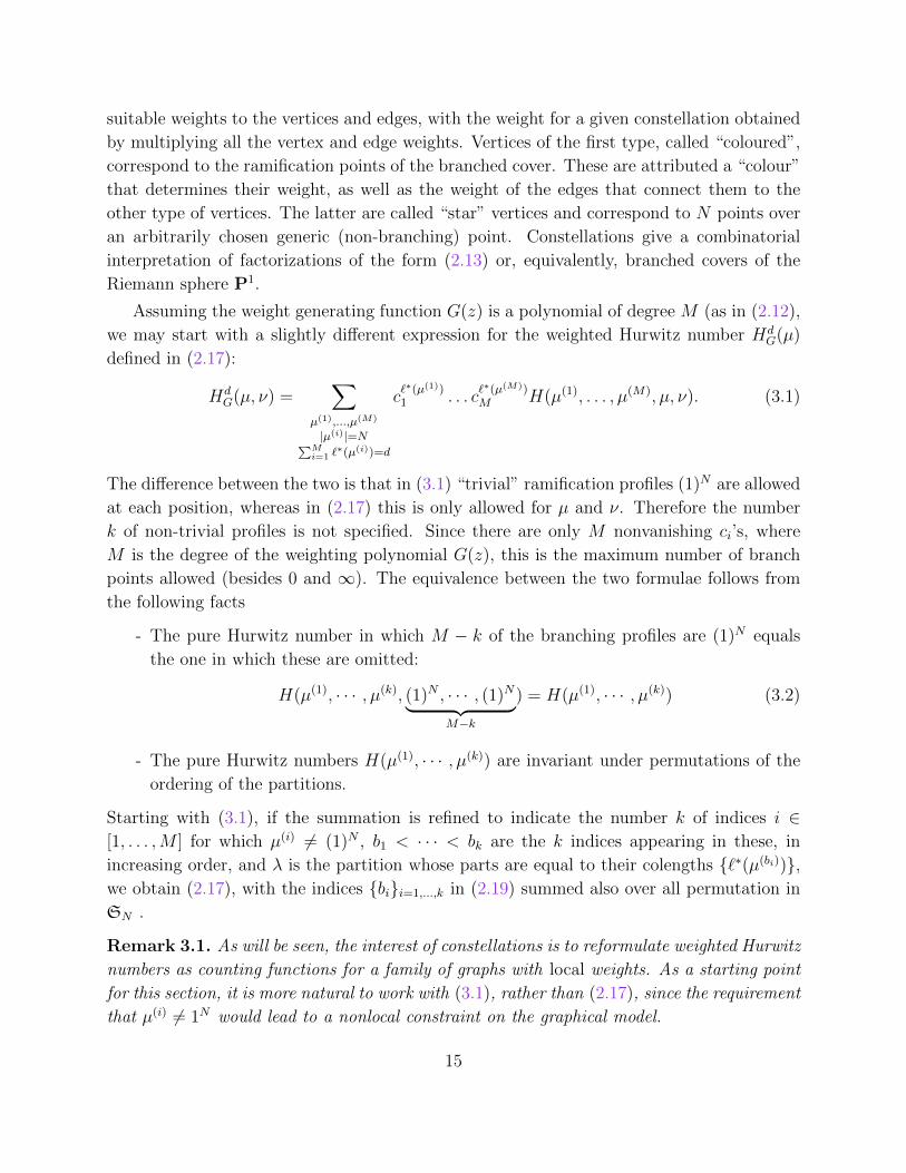
Definition 3.1. An M+2-constellation of size N is a graph embedded in a compact oriented
surface, in such a way that each face is homeomorphic to a disk, considered up to oriented
homeomorphism. It consists of the following data and constraints:
- There are two kinds of vertices: star vertices, of which there are N in total, numbered
consecutively from 1 to N , and coloured vertices. Each coloured vertex carries a colour,
labelled by M + 2 indices (0, . . . ,M,M + 1), but several different vertices can have the
same colour.
- Each edge links a star vertex to a coloured vertex.
- Each star vertex has degree M + 2, and the sequence of colours of its neighbours in
counterclockwise order is 0, 1, . . . ,M,M + 1.
- Each face contains exactly one angular sector of each colour (equivalently it is bounded
by 2(M + 2) edge sides).
(See Figure 1 for an example where N = 5,M = 3.)
The colour 0 and the last colour, M + 1, play a special role; anticipating the covering
interpretation given in Section 3.4, we also denote the last colour M +1 as∞ (see Figure 1).
We now explain the relation between constellations and Hurwitz numbers. Given an
M + 2-constellation of size N , define the permutations (h0, h1, . . . , hM , hM+1) in SN by
hi(j) := j′, where j′ is the label of the star vertex following the star vertex labelled j clockwise
around its unique neighbour of colour i. In other words, each cycle of the permutation higives the clockwise order of appearance of star vertices around a vertex of colour i. It
is easy to see that the distinct cycles of the elements h0, h1, . . . , hM+1 are in one-to-one
correspondence with the faces of the graph on the surface and that the product h0h1 . . . hM+1
is the identity. (See Figure 1.) Clearly this construction can be inverted; given an (M + 2)-
tuple of permutations whose product is the identity, one can reconstruct a unique embedded
graph as in Definition 3.1 by gluing together vertices in accordance with the rules. Therefore
we have
Lemma 3.1 (see [54, Chapter 1]). The Hurwitz number H(µ(1), . . . , µ(M), µ, ν) is 1N !
times
the number of constellations with N star vertices such that the partition of N giving the
degrees of the vertices of colour i is µ(i) for 0 ≤ i ≤M + 1, with µ(0) = µ, µ(M+1) = ν.
Note that the Euler characteristic χ of the surface is given by the Riemann-Hurwitz
formula (cf. eq. (2.15))
χ = 2− 2g = `(µ) + `(ν)−M∑i=1
`∗(µ(i)). (3.3)
16
3
2
3
0
3
1
2
0
12
3
4
1
3
0
5
∞
∞
∞∞
2
1
Figure 1: An example of a constellation with N = 5, M = 3. We use ∞ to denote the last colourM+1 = 4. The example corresponds to the factorization h0h1h2h3h4 = 1 with h0 = (123), h1 = (153), h2 =(15)(23), h3 = (14), h4 = h∞ = (14), with corresponding partitions µ(1) = (3, 1, 1)), µ(2) = (2, 2, 1), µ(3) =(2, 1, 1, 1), µ := µ(0) = (3, 1, 1)), ν := µ(4) = (2, 1, 1, 1). In the picture elements of the ground set 1, . . . , Nare indicated with underlined numbers, while numbers corresponding to colours are not underlined. Thisexample has genus g = 0.
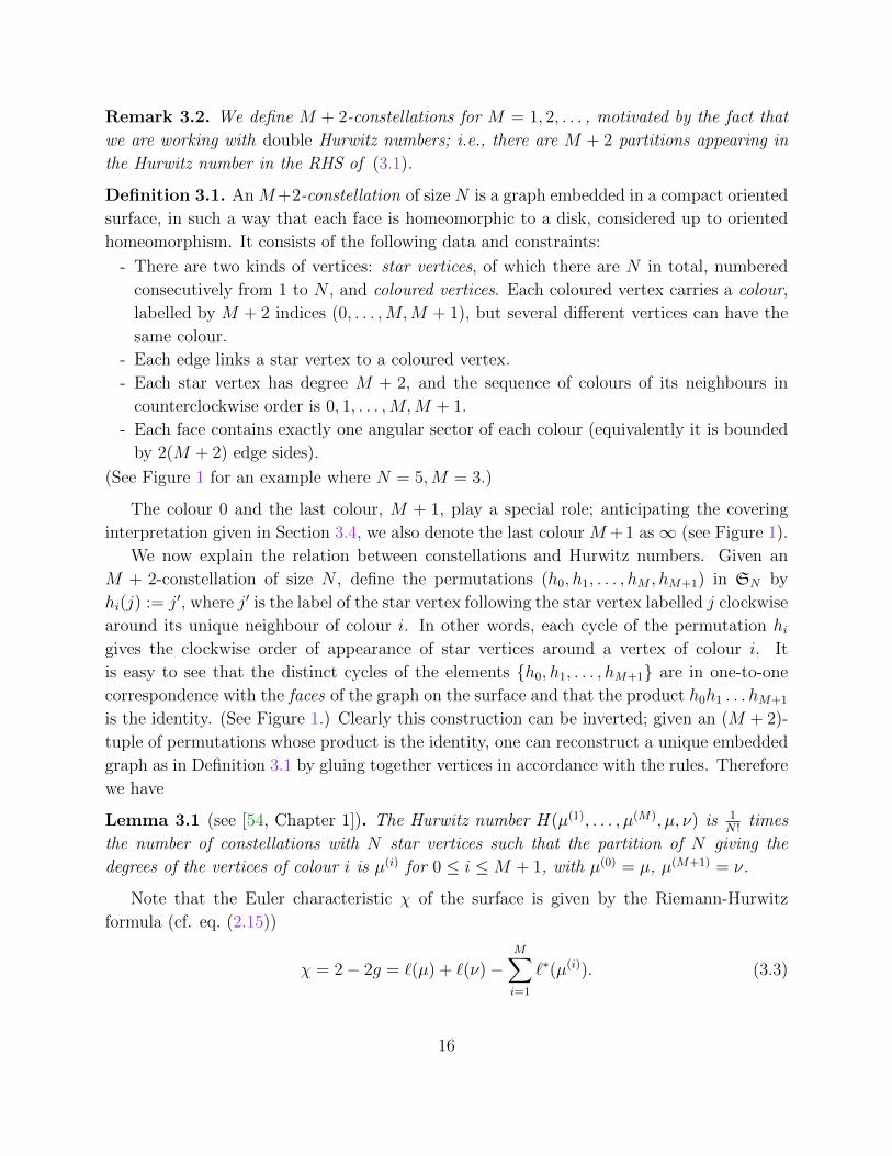
3.2 Weighted constellations
We now turn to the weighting of the vertices and edges of a given constellation that will
enable us to view the τ -function as a generating function for constellations. Recall that
the colours are labelled 1, . . . ,M where M is the degree of G(z), plus two special colours,
white and black, corresponding to 0 and ∞, respectively, in the branched covering surface
interpretation. (See subsection 3.4 for details of this correspondence and Figures 2, 3 for a
visualization of the weighting scheme.)
- Coloured vertices. To the ordinary coloured vertices of colour i for 1 ≤ i ≤ M , we
assign a weight (βci)−1. To the edges linking them to the star vertices, we assign a
weight βci.
- White vertices. To the white vertices (of colour 0), we assign the power sum symmetric
functions pj = jtj, where j is the vertex degree. The edges that connect them to the
star vertices have weight 1.
- Black vertices. To the black vertices (of colour∞), we assign the power sum symmetric
functions pj = jsj, where j is the vertex degree. The edges that connect them to the
star vertices have weight 1.
- Star vertices Finally, to each of the N star vertices we assign a weight γ.
17
(βci)−1
γ
γ
γγ
γ
βciβc i
βci
i
βci
βci
pj(t)
γ
γ
γγ
γ
degree j
0 pj(s)
γ
γ
γ
∞
γ
γ
degree j
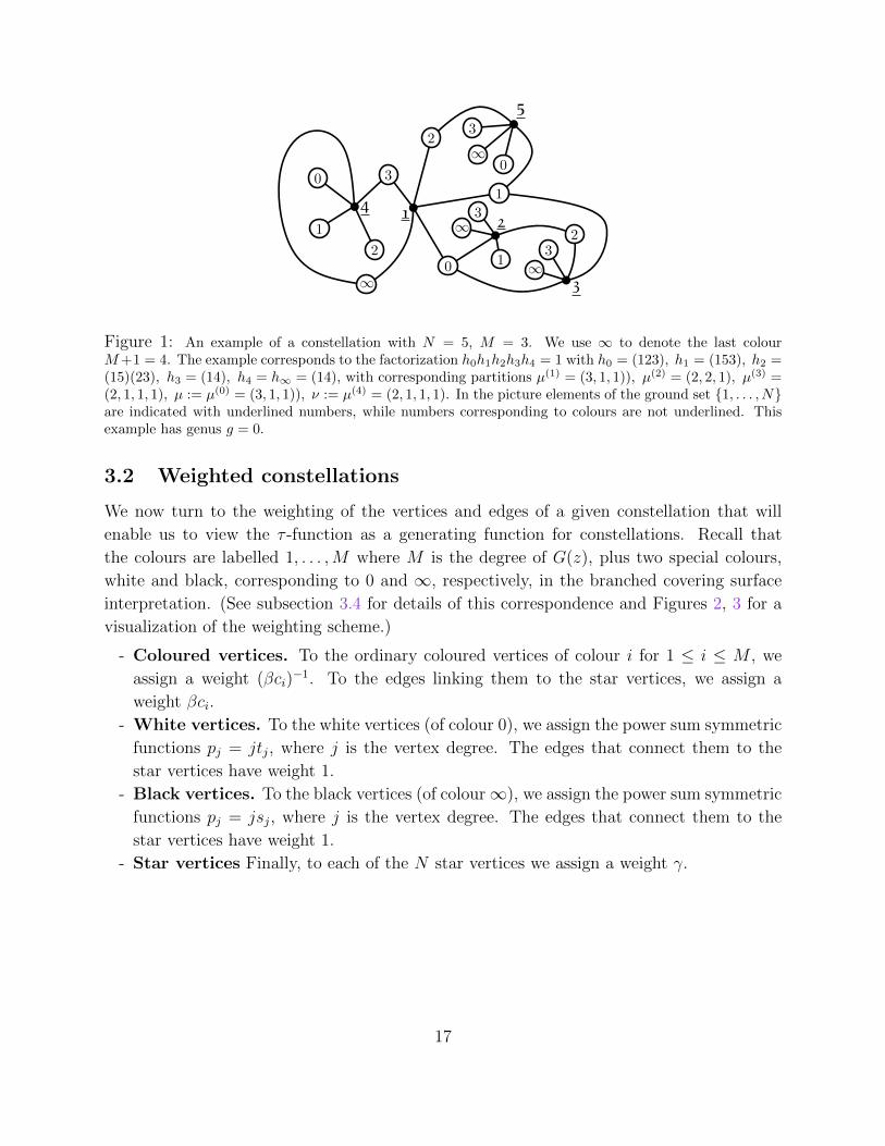
Figure 2: Weights. Left: coloured vertices and edges. Center: white vertices. Right: black vertices. Thevertex degree is j = 5 on the center and right examples.
3.3 Reconstructing the τ-function
Taking the product over all the weights gives the total weight for the constellation as
γNβdM∏i=1
(ci)`∗(µ(i))pµ(t)pν(s), (3.4)
where d is given by (2.16). Summing the contributions of all constellations, and using (3.1)
and Lemma 3.1, we recognise the expression (2.26) for the τ -function and obtain:
Proposition 3.2. The function τ (G,β,γ)(t, s) ∈ K[t, s, β][[γ]] is the exponential generating
function of weighted (M + 2)-constellations.
Recall that here, “exponential” generating function means that each constellation is
counted with an extra factor of 1N !
. Since each constellation can be uniquely decomposed
into connected components, the exp-log principle (see e.g. [31]) ensures that ln τ (G,β,γ)(t, s)
is the generating function of connected constellations, with the same weighting scheme as
in Proposition 3.2. (A constellation is connected if and only if its underlying surface is.)
Equivalently, in the notation of weighted Hurwitz numbers we have:
ln τ (G,β,γ)(t, s) :=∑µ,ν|µ|=|ν|
γ|µ|∑d
βdHdG(µ, ν) pµ(t)pν(s). (3.5)
where HdG(µ, ν) denotes the connected weighted Hurwitz number (see [6, 7, 39,41]).
3.4 Direct correspondence between constellations and coverings
For completeness, we recall in this section how the link between constellations and branched
covers can be made directly, without relying on permutations. This well-known correspon-
dence (see again [54, Chapter 1]) enables us to draw the graph directly on the surface of
18
...
(βci)−1
βci
βci
βci
Q(i)
`(µ(i))
Q(i)1
Q(i)
...
(βci)−1
(βci)−1
Q(i)j
...
i
i
i
γ
γ
γ
...
pµ(0)j
(t)
Q(0)
`(µ(0))
Q(0)1
Q(0)
...
Q(0)j
...
0
0
0
γ
γ
γ
...
pµ(∞)j
(s)
Q(∞)
`(µ(∞))
Q(∞)1
Q(∞)
...
Q(∞)j
...
∞
∞
∞
γ
γ
γ
...
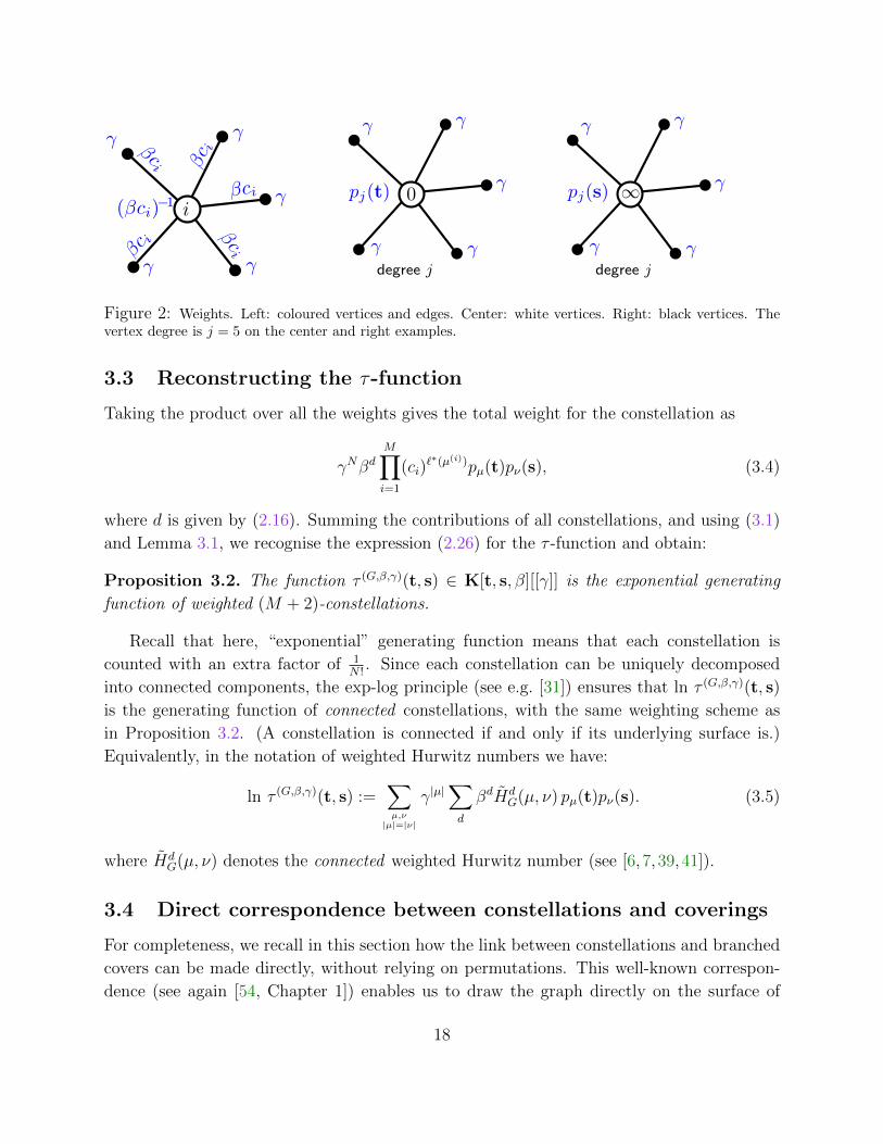
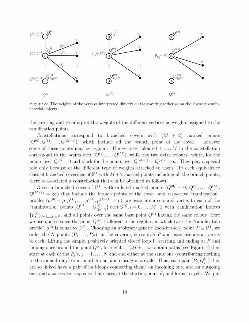
Figure 3: The weights of the vertices interpreted directly on the covering rather as on the abstract combi-natorial objects.
the covering and to interpret the weights of the different vertices as weights assigned to the
ramification points.
Constellations correspond to branched covers with (M + 2) marked points
(Q(0), Q(1), . . . , Q(M+1)), which include all the branch point of the cover – however
some of these points may be regular. The vertices coloured 1, . . . ,M in the constellation
correspond to the points over (Q(1), . . . , Q(M)), while the two extra colours: white, for the
points over Q(0) = 0 and black for the points over Q(M+1) = Q(∞) =∞. They play a special
role only because of the different type of weights attached to them. To each equivalence
class of branched coverings of P1 with M + 2 marked points including all the branch points,
there is associated a constellation that can be obtained as follows.
Given a branched cover of P1, with ordered marked points (Q(0) = 0, Q(1), . . . , Q(M),
Q(M+1) = ∞) that include the branch points of the cover, and respective “ramification”
profiles (µ(0) = µ, µ(1), . . . , µ(M), µ(M+1) = ν), we associate a coloured vertex to each of the
“ramification” points Q(i)1 , . . . Q
(i)
`(µ(i)) overQ(i), i = 0, . . . ,M+1, with “ramification” indices
µ(i)j j=1,...,`(µ(i)) and all points over the same base point Q(i) having the same colour. Here
we use quotes since the point Q(i) is allowed to be regular, in which case the “ramification
profile” µ(i) is equal to [1N ]. Choosing an arbitrary generic (non-branch) point P ∈ P1, we
order the N points (P1, . . . , PN), in the covering curve over P and associate a star vertex
to each. Lifting the simple, positively oriented closed loop Γi starting and ending at P and
looping once around the point Q(i), for i = 0, . . . ,M + 1, we obtain paths (see Figure 4) that
start at each of the Pj’s, j = 1, . . . , N and end either at the same one (contributing nothing
to the monodromy) or at another one, and closing in a cycle. Thus, each pair (Pj, Q(i)j ) that
are so linked have a pair of half-loops connecting them: an incoming one, and an outgoing
one, and a successive sequence that closes at the starting point Pj and forms a cycle. We put
19

an edge connecting (Pj, Q(i)k ) for each such pair for which there are loops that are part of a
cycle. The product of the disjoint cycles over a given point defines the corresponding element
hi ∈ SN , which has cycle lengths given by the parts of the partition µ(i). All “ramification
points” Q(i)j j=1...,`(µ(i)) over a given point Q(i) correspond to a coloured vertex, with colour
i, and each of the points Pjj=1,...,N corresponds to a star vertex. The resulting graph is
the constellation corresponding to the given branched cover.
Q(i)
`(µ(i))
Q(i)1
Q(i)
Q(i)j
P
Pa
Pb
Pc
(a, b, c)
Figure 4: Lifted loops and edges. Here, (a, b, c) represents a (typical) cycle in the monodromy factorizationat the indicated branch point.
4 Fermionic and bosonic functions
In much of the following, we denote τ (G,β,γ)(t, β−1s) simply as τ(t), viewing the parameters
(c1, c2, . . . ) defining G as well as β, γ and s all as auxiliary parameters. The fact that this
is the n = 0 lattice point evaluation of a 2D-Toda τ -function when the s variables are taken
as independent does not play any role in this section, and the second set of flow variables
s = (s1, s2, . . . ) are viewed as auxiliary parameters in a KP τ -functions, which serve as
book-keeping parameters in the generating function interpretation. Most of the definitions
and several of the results of the following three subsections are, in fact, valid for completely
general functions τ(t), whether they are KP τ -functions, or not. The sole exceptions are
Propositions 4.1 and 4.5, which are valid for any KP τ -function τ(t), and Propositions 4.2 and
4.8, which are only valid for the specific τ -functions τ (G,β,γ)(t, β−1s) defined by eqs. (2.22),
(2.26).
20

4.1 Fermionic functions
The functions defined in this subsection will be referred to as fermionic functions. The
definitions remain valid regardless of whether or not τ(t) is a KP τ -function, but Proposition
4.1 only holds true if it is (regardless of which KP τ -function it is). In this case, their
representation as vacuum expectation values (VEV’s) of products of fermionic operators is
given in [7].
The first of these is the Baker function and its dual, which will be denoted Ψ−(G,β,γ)(ζ, t, s)
and Ψ+(G,β,γ)(ζ, t, s), respectively, and are given by the Sato formulae
Ψ∓(G,β,γ)(ζ, t, s) = e±∑∞i=1 tiζ
i τ (G,β,γ)(t∓ [x], s)
τ(t, s)= e±
∑∞i=1 tiζ
i
(1 +O(1/ζ)) , (4.1)
where ζ is the spectral parameter.
x := ζ−1 (4.2)
and [x] is the infinite vector whose components are equal to the terms of the Taylor expansion
of − ln(1− x) at x = 0
[x] :=
(x,x2
2, . . . ,
xn
n, . . .
). (4.3)
We view the Baker function and its dual as associated to the family of KP τ -functions
τ(t) in the flow variables t = (t1, t2, . . . ) with (β, γ), c = (c1, c2, . . . ) and s = (s1, s2, . . . )
interpreted as parameters. The expansion of the Baker function Ψ−(G,β,γ)(ζ, t, s) and its dual
Ψ+(G,β,γ)(ζ, t, s) in terms of the bases Ψ+
−kk∈N and Ψ−−kk∈N for the subspaces W (G,β,γ,s)⊥
and W (G,β,γ,s), respectively, is given in the companion paper [7].
Note that, from the Sato formulae (4.1), and the expansion (2.26) of the τ -function, we
have the following expansion of the t = 0 values of Ψ±(G,β,γ)(ζ, t, s) as a Taylor series in the
spectral parameter and a power sum series in the parameters s, with the weighted Hurwitz
numbers as coefficients
Ψ±0 (x) := Ψ±(G,β,γ),(x−1,0, β−1s
)=∑µ,ν
∑d
(xγ)|µ|(±1)`(µ)βd−`(ν)HdG(µ, ν) pν(s). (4.4)
More generally, for any KP τ -function τ(t), by Sato’s formula, evaluation of the Baker
function at t = 0 is given by
Ψ±0 (x) = τ(±[x]). (4.5)
Definition 4.1. For an arbitrary KP τ -function τ(t) (in particular, for the choice τ(t) =
τ (G,β,γ)(t, β−1s)), the pair correlator is defined as
K(x, x′) :=1
x− x′ τ([x]− [x′]
), (4.6)
21
and for n ≥ 1, the n-pair correlator is
Kn(x1, . . . , xn;x′1, . . . , x′n) := det
(1
xi − x′j
)1≤i,j≤n
× τ(∑
i
[xi]− [x′i]
). (4.7)
Remark 4.1. The justification for this terminology is that, when τ(t) is a KP τ -function,
these quantities are all expressible as fermionic VEV’s involving products of n pairs of
creation and annihilation operators, as detailed in [7]. We note that in the particular
case where τ(t) = τ (G,β,γ)(t, β−1s), Ψ±0 (x) ∈ K[x, s, β, β−1][[γ]], while for any n ≥ 1,
Kn(x1, . . . , xn;x′1, . . . , x′n) ∈ K(x1, . . . , xn, x
′1, . . . , x
′n)[s, β, β−1][[γ]].
The following result is standard, and follows from the Cauchy-Binet identity (or, equiv-
alently, the fermionic Wick theorem). A proof, valid for all KP τ -functions, is given in the
appendix of [7].
Proposition 4.1. We have
Kn(x1, . . . , xn;x′1, . . . , x′n) = det
(K(xi, x
′j)). (4.8)
4.2 Bosonic functions
Define the following derivations:
Definition 4.2. For any parameter x
∇(x) :=∞∑i=1
xi−1∂
∂ti, ∇(x) :=
∞∑i=1
xi
i
∂
∂ti(4.9)
In terms of these, and any function τ(t) of the infinite sequence t = (t1, t2, . . . ) of flow
variables (in particular, for the choice τ(t) = τ (G,β,γ)(t, β−1s)), we introduce the following
correlators
Wn(x1, . . . , xn) :=
(( n∏i=1
∇(xi))τ(t)
)∣∣∣∣∣t=0
, (4.10)
Wn(x1, . . . , xn) :=
(( n∏i=1
∇(xi))
ln τ(t)
)∣∣∣∣∣t=0
, (4.11)
Fn(x1, . . . , xn) :=
(( n∏i=1
∇(xi))τ(t)
)∣∣∣∣∣t=0
, (4.12)
Fn(x1, . . . , xn) :=
(( n∏i=1
∇(xi))
ln τ(t)
)∣∣∣∣∣t=0
. (4.13)
22
Remark 4.2. Note that these definitions apply equally for any function τ(t) admitting a
formal, or analytic, power series expansion in the flow parameters t = (t1, t2, . . . ), since they
only refer to the dependence on these parameters, whereas the parameters s = (s1, s2, . . . )
are just present as “spectator” parameters within the definition.
It follows that
Wn(x1, . . . , xn) =∂
∂x1. . .
∂
∂xnFn(x1, . . . , xn), (4.14)
Wn(x1, . . . , xn) =∂
∂x1. . .
∂
∂xnFn(x1, . . . , xn). (4.15)
As shown in [7], if τ(t) is a KP τ -function, Wn(x1, . . . , xn) has a fermionic representation as
a multicurrent correlator.
Assuming τg(t) to be normalized such that τg(0) = 1, we have, in particular,
W1(x1) = W1(x1)
W2(x1, x2) = W2(x1, x2)−W1(x1)W2(x2)
W3(x1, x2, x3) = W3(x1, x2, x3)−W1(x1)W2(x2, x3)−W1(x2)W2(x1, x3)−W1(x3)W2(x1x2)
+ 2W1(x1)W1(x2)W1(x3)... =
... (4.16)
For general n, the moment/cumulant relations between connected and nonconnected func-
tions give
Wn(x1, . . . , xn) =∑`≥1
∑I1]···]I`=1,...,n
∏i=1
W|Ii|(xj, j ∈ Ii), (4.17)
with identical relations holding between the Fn’s and Fn’s.
For the particular case of τ -functions τ (G,β,γ)(t, β−1s) with expansion (2.26), we write:
Wn(x1, . . . , xn) = Wn(s; β; γ;x1, . . . , xn), Wn(x1, . . . , xn) = Wn(s; β; γ;x1, . . . , xn),
(4.18)
Fn(x1, . . . , xn) = Fn(s; β; γ;x1, . . . , xn), Fn(x1, . . . , xn) = Fn(s; β; γ;x1, . . . , xn)
(4.19)
It follows that the Fn’s and Fn’s may also be viewed as generating functions for the weighted
Hurwitz numbers HdG(µ, ν), encoding the same information as τ (G,β,γ)(t, β−1s), but in a
different way.
23
Proposition 4.2.
Fn(s; β; γ;x1, . . . , xn) =∞∑d=0
∑µ,ν,|µ|=|ν|`(µ)=n
γ|µ|βd−`(ν)HdG(µ, ν) | aut(µ)|mµ(x1, . . . , xn)pν(s),
(4.20)
Fn(s; β; γ;x1, . . . , xn) :=∞∑d=0
∑µ,ν,|µ|=|ν|`(µ)=n
γ|µ|βd−`(ν)HdG(µ, ν) | aut(µ)|mµ(x1, . . . , xn)pν(s)
(4.21)
=∞∑g=0
β2g−2+nFg,n(s, γ;x1, . . . , xn),
(4.22)
where
Fg,n(s; γ;x1, . . . , xn) =∑
µ,ν,|µ|=|ν|`(µ)=n
γ|µ|H2g−2+n+`(ν)G (µ, ν) | aut(µ)|mµ(x1, . . . , xn)pν(s) (4.23)
and mµ(x1, . . . , xn) is the monomial symmetric polynomial in the indeterminates (x1, . . . , xn).
Proof. Applying the operator∏n
i=1 ∇(xi) to the symmetric function pµ(t) in the expansion
(2.26) gives(n∏i=1
∇(xi)
)pµ(t)
∣∣∣∣∣t=0
=n∏i=1
(∞∑ji=1
1
jixjii
∂
∂tji
)`(µ)∏k=1
µktµk
∣∣∣∣∣∣t=0
= δ`(µ),n∑σ∈Sn
n∏k=1
xµkσ(k) = δ`(µ),n| aut(µ)|mµ(x1, . . . , xn) (4.24)
by (2.19). Hence, applying it to τ (G,β,γ)(t, β−1s), using the expansion (2.26), we obtain from
the definition (4.12) of Fn(s, x1, . . . , xn)
Fn(s; β; γ;x1, . . . , xn) =∑
µ,ν, `(µ)=n
∑d
γ|µ|βd−`(ν)HdG(µ, ν)| aut(µ)|mµ(x1, . . . , xn)pν(s),
(4.25)
proving (4.20). The same calculation proves the connected case (4.23).
Note that Fn(s; β; γ;x1, . . . , xn) and Fn(s; β; γ;x1, . . . , xn) belong to K[x1, . . . , xn; s; β, β−1][[γ]]
while the Fg,n(s; γ;x1, . . . , xn)’s are in K[x1, . . . , xn; s][[γ]]. We also define
Wg,n(s; γ;x1, . . . , xn) :=∂
∂x1. . .
∂
∂xnFg,n(s; γ;x1, . . . , xn) (4.26)
24
and therefore, from eq. (4.22), we have the expansion
Wn(s; β; γ;x1, . . . , xn) =∞∑g=0
β2g−2+nWg,n(s, γ;x1, . . . , xn). (4.27)
In the following two subsections, we give explicit relations between the functions defined
above. Note that these relations hold in complete generality, valid for pair correlators and
current correlators defined by the formulae (4.7), (4.10) - (4.13) for arbitrary τ -functions.
Propositions 4.3 and 4.4 are in fact tautological; they do not even require that τ(t) be a KP
τ -function.
4.3 From bosons to fermions
The following proposition allows us to write the fermionic functions in terms of the bosonic
ones. We emphasize that it does not even require τ(t) to be a KP τ -function, just an infinite
power series in the flow variables t, whether formal or analytic.
Proposition 4.3. For all τ(t) admitting an analytic or formal power series expansion in the
parameters t = (t1, t2, . . . ), with Ψ±0 (x) defined by (eq. 4.5) and Kn(x1, . . . , xn;x′1, . . . , x′n) by
(4.7), we have
Ψ±0 (x) =∑n
(±1)n
n!Fn(x, . . . , x)
= e∑n
(±1)n
n!Fn(x,...,x), (4.28)
K(x, x′) =1
x− x′∑n,m
(−1)m
n!m!Fn+m(
n︷ ︸︸ ︷x, . . . , x,
m︷ ︸︸ ︷x′, . . . , x′)
=1
x− x′ e∑n,m
(−1)m
n!m!Fn+m(
n︷ ︸︸ ︷x, . . . , x,
m︷ ︸︸ ︷x′, . . . , x′).
(4.29)
More generally, we have
Kk(x1, . . . , xk;x′1, . . . , x
′k)/det
(1
xi − x′j
)
=∑
n1,...,nk,m1,...,mk
(−1)∑imi∏
i ni!∏
imi!F∑
i ni+mi(. . . ,
ni︷ ︸︸ ︷xi, . . . , xi, . . . ,
mj︷ ︸︸ ︷x′j, . . . , x
′j, . . . ) (4.30)
= exp
∑n1,...,nk,m1,...,mk
(−1)∑imi∏
i ni!∏
imi!F∑
i ni+mi(. . . ,
ni︷ ︸︸ ︷xi, . . . , xi, . . . ,
mj︷ ︸︸ ︷x′j, . . . , x
′j, . . . )
.(4.31)
25
Remark 4.3. For the case τ(t) = τ (G,β,γ)(t, β−1s) with expansion (2.26), these equalities
should be interpreted in K(x, x′;xi, x′i, 1 ≤ i ≤ n)[s, β, β−1][[γ]]. Substituting the genus ex-
pansion (4.22) for Fn(s; γ;x1, . . . , xn) into the exponential sums in (4.28), (4.29) and (4.31)
gives the genus expansions of the latter.
Proof. All the results stated follow from the single tautological identity
e∑ki=1 ∇(xi)−
∑lj=1 ∇(yj)τ(t)|t=0 = τ(
k∑i=1
[xi]−l∑
j=1
[yj]), (4.32)
valid for any infinitely differentiable function τ(t) of an infinite sequence of variables t =
(t1, t2, . . . ), or formal power series in these variables, and any set of k + l indeterminates
(x1, . . . , xk, y1, . . . , yl), by expanding the exponential series for each term in the exponent
sum of (commuting) operators. For the case Ψ±0 (x), to obtain (4.28) we recall eq. (4.5), and
choose either k = 1, l = 0, x1 = x or k = 0, l = 1, y1 = x in (4.32). The case (4.31) is
obtained by doing the same for k = l, and setting the yi = x′i, i = 1, . . . , k. The connected
versions follow from applying the same exponential of commuting operators to ln(τ(t)).
4.4 From fermions to bosons
Conversely to the results of the previous subsections, we can also express the bosonic func-
tions in terms of the fermionic ones. The next result is again valid for any function τ(t) admit-
ting either a convergent or formal power series expansion in the flow variables t = (t1, t2, . . . ).
Proposition 4.4.
Wn(x1, . . . , xn) = [ε1 . . . εn](Kn(x1, . . . , xn;x1 − ε1, . . . , xn − εn)
/det(
1xi−xj+εj
)), (4.33)
Proof. From the definition (4.7), this is equivalent to the relation
∂n τ(∑n
i=1 ([xi]− [xi − εi]))∂ε1 · · · ∂εn
∣∣∣∣εi=0i=1,...,n
=n∏i=1
∇(xi)τ(t)|t=0, (4.34)
which follows from1
j((xi)
j − (xi − εi)j) = εixj−1i +O(ε2i ) (4.35)
by applying the chain rule.
If τ(t) is a KP τ -function, by Proposition 4.1, the n-pair correlatorKn(x1, . . . , xn;x′1, . . . , x′n)
is expressible as an n× n determinant in terms of the single pair correlators K(xi, x′j). This
enables us to express the functions Wn in terms of these quantities alone. For the connected
functions, Wn(x1, . . . , xn), we get specially elegant relations.
26
Proposition 4.5.
W1(x) = limx′→x
(K(x, x′)− 1
x− x′), (4.36)
W2(x1, x2) =
(−K(x1, x2)K(x2, x1)−
1
(x1 − x2)2), (4.37)
and for n ≥ 3
Wn(x1, . . . , xn) =∑
σ∈S1−cyclen
sgn(σ)∏i
K(xi, xσ(i)), (4.38)
where the last sum is over all permutations in Sn consisting of a single n-cycle.
Proof. The proof is given in Appendix A.1. It is based on a computation of the exact
expression for the unconnected correlator Wn(x1, . . . , xn), using the determinantal identity
(4.8), followed by application of the cumulant identity (4.17) relating this to the connected
correlators Wk(x1, . . . , xn)k=1,...,n
Remark 4.4. Such relations were first noted in the context of complex matrix models [12].
If we view eqs. (4.5), (4.7) , (4.10), (4.12) (4.13), as definitions of the functions Ψ±0 (x),
Kn(x1, . . . , xn, x′1, . . . , x
′n), Wn(x1, . . . , xn), Fn(x1, . . . , xn) and Fn(x1, . . . , xn), respectively,
Propositions 4.3 and 4.4 are valid for completely arbitrary functions τ(t) admitting ei-
ther a formal or convergent power series expansion in the variables t = (t1, t2, . . . ), while
Proposition 4.5 remains valid if Wn(x1, . . . , xn) is defined by (4.11) in terms of an arbitrary
KP τ -function τ(t).
Remark 4.5. For the case τ(t) = τ (G,β,γ)(t, β−1s) with expansion (2.26), these equalities
should be interpreted as being in K(x, x′;xi, x′i, 1 ≤ i ≤ n)[s, β, β−1][[γ]].
4.5 Expansion of K(x, x′) for the case τ (G,β,γ)(t, β−1s)
Some properties of Schur functions corresponding to hook partitions will be needed in the
following (see [55]):
Lemma 4.6. The Schur function s(a|b)(t) corresponding to a hook partition (1 + a, 1b), (de-
noted (a|b) in Frobenius notation) may be expressed in terms of the complete symmetric
functions as
s(a|b)(t) =b+1∑j=1
ha+j(t)hb−j+1(t). (4.39)
Substituting the specific evaluations at t = [x]− [x′], we obtain
Lemma 4.7. The Schur function sλ([x] − [x′]) vanishes unless λ is a hook or the trivial
partition and in that case it takes the value
s(a|b)([x]− [x′]) = (x− x′)xa(−x′)b. (4.40)
27
From (4.6), (2.22) and Lemma 4.7 we obtain (see [6] for details of the proof):
Proposition 4.8. For the particular case where τ(t) = τ (G,β,γ)(t, β−1s), the correlation
function K(x, x′) can be expressed as:
K(x, x′) =1
x− x′ +∑a,b≥0
ρaρ−1−b−1x
a(−x′)bs(a|b)(β−1s)
=1
x− x′ +∞∑a=0
∞∑b=0
b+1∑j=1
ρaha+j(β−1s)xaρ−1−b−1hb−j+1(−β−1s)(x′)b. (4.41)
5 Adapted bases, recursion operators and the
Christoffel-Darboux relation
5.1 Recursion operators and adapted basis
In this section we describe, for the case of the τ -function τ (G,β,γ)(t, β−1s), an alternative
approach to the adapted bases Ψ+i (x)i∈Z and their duals Ψ−i (x)i∈Z. All subsequent de-
velopments concern only this specific case: the hypergeometric τ -function τ (G,β,γ)(t, β−1s)
defined in (2.22) which serves, by (2.26), as generating function for weighted Hurwirz num-
bers.
Definition 5.1. Denote the Euler operator as
D := xd
dx(5.1)
and define the pair of dual recursion operators
R± := γxG(±βD). (5.2)
The same operators in the variable x′ are denoted D′ and R′±
Since D commutes with G(±βD), it follows that these operators satisfy the commutation
relations
[D,R±] = R±. (5.3)
Definition 5.2. Denote the (normalized) power sums of the variables cii∈N+ :
Ak :=1
k
∞∑i=1
cki , k > 0. (5.4)
Then the following lemma is easily proved (see Appendix A.2).
28
Lemma 5.1. There exists a unique formal power series T (x) such that
eT (x)−T (x−1) = γG(βx) (5.5)
with T (x)− x log γ ∈ K[x][[β]] and T (0) = 0. Explicitly,
T (x) = x log γ +∞∑k=1
(−1)kAkβkBk+1(x)−Bk+1(0)
k + 1. (5.6)
where Bk(x) are the Bernoulli polynomials.
Corollary 5.2. The operators R± can be expressed as
R+ = eT (D−1) x e−T (D−1), (5.7)
R− = e−T (−D) x eT (−D). (5.8)
We can now express the Baker function Ψ−0 (x) and its dual Ψ+0 (x), as well as K(x, x′),
in terms of the series T . Defining
ξ(x, s) :=∞∑k=1
skxk, (5.9)
we have
Proposition 5.3.
Ψ+0 (x) = γeT (D−1)
(eβ−1ξ(x,s)
), (5.10)
Ψ−0 (x) = e−T (−D)(e−β
−1ξ(x,s)), (5.11)
K(x, x′) = eT (D)−T (−D′−1)
(eβ−1ξ(s,x)−β−1ξ(s,x′)
x− x′
). (5.12)
Proof. From the Cauchy-Littlewood identity and Lemma 4.7 we have
∑a,b≥0
xa(−x′)bs(a|b)(β−1s) =eβ−1ξ(s,x)−β−1ξ(s,x′)
x− x′ . (5.13)
Expression (5.12) forK(x, x′) then follows from the definition of the operators T (D), T (D−1)
and Proposition 4.8. The other two equalities are proved similarly.
Definition 5.3. Using the operators R± defined in (5.2), we define
Ψ±k (x) := Rk±Ψ±0 (x), k ∈ Z. (5.14)
29
It then follows from (5.7) that
Proposition 5.4.
Ψ+k (x) = γeT (D−1)
(xk eβ
−1ξ(x,s)), (5.15)
Ψ−k (x) = e−T (−D)(xk e−β
−1ξ(x,s)). (5.16)
and we have the following identifications:
Proposition 5.5. The functions Ψ±k (x)k∈Z defined in (5.14) coincide with those defined
in (2.36) and (2.37). Thus we have the series expansions
Ψ+k (x) = γ
∞∑j=0
xj+khj(β−1s)ρj+k−1, (5.17)
Ψ−k (x) =∞∑j=0
xj+khj(−β−1s)ρ−1−j−k. (5.18)
Proof. From the definition 2.10 of the coefficients ρj it follows that
eT (D−1)xk = ρk−1xk (5.19)
e−T (−D)xk = ρ−1−kxk. (5.20)
The statement then follows from the series expansion of the expressions in the parentheses
in (5.15)-(5.16).
Remark 5.1. The operator representation (5.15), (5.16) coincides with the generalized con-
volution action on the standard orthonormal (monomial basis) elements of H, as explained in
Section 2.3, and given in eqs. (2.36), (2.37). Using different methods, the series expansions
(5.17), (5.18) were also derived in the companion papers [6, 7].
From (5.15), (5.16) we deduce
Proposition 5.6. For all m > 0 and k ∈ Z, we have
Ψ±k+m(x) = ±β d
dsmΨ±k (x). (5.21)
Proof. This follows from the series expansions (5.17) (5.18) using the property
∂hj(s)
∂si= hj−i(s). (5.22)
30
5.2 The Christoffel-Darboux relation
Definition 5.4. Define the quantity S(z) by
S(z) := zd
dzξ(z, s) =
∞∑k=1
kskzk. (5.23)
In the following, we assume that only a finite number of variables sk are nonzero; i.e.,
that S(z) is a polynomial in z of degree
L := degS. (5.24)
We also assume that the model is not degenerate; i.e., ML > 1.
Definition 5.5. Define the operators
∆±(x) := ±βe∓β−1ξ(x,s) D e±β−1ξ(x,s) = S(x)± βD (5.25)
and
V±(x) := γ−1x−1e∓β−1ξ(x,s) R± e±β
−1ξ(x,s) = G(∆±(x)). (5.26)
Definition 5.6. The polynomial A(r, t) of degree LM − 1 in each variable (r, t) and the
LM × LM matrix A = (Aij)0≤i,j≤LM−1 are defined by
A(r, t) := (r V−(t)− t V+(r))
(1
r − t
)=
LM−1∑i=0
LM−1∑j=0
Aijritj. (5.27)
The highest total degree term is
gM (LsL)Mr tLM − t rLM
r − t = −gM (LsL)MLM−1∑j=1
rjtLM−j, (5.28)
so
detA = (−1)LM(LM−1)
2 gLM−1M (LsL)M(LM−1). (5.29)
Therefore the matrix A is nonsingular.
The following two results are proved in [7]. For the convenience of the reader, a short
proof of the first result using only the notation of the present paper is also given in Appendix
A.2.
Theorem 5.7 ( [7]). The following “Christoffel-Darboux” relation holds:
K(x, x′) =1
x− x′A(R+, R′−)Ψ+
0 (x)Ψ−0 (x′) =1
x− x′LM−1∑i,j=0
AijΨ+i (x)Ψ−j (x′). (5.30)
31
Proposition 5.8 ( [7]). The Christoffel-Darboux matrix elements Aij entering in (5.27)
have the explicit expression
Aij = −j∑
k=−i
G(kβ)hj−k(−β−1s)hi+k(β−1s), i, j = 1, 2, . . . , (5.31)
A00 = 1, A0j = Ai0 = 0.
For example, if L = M = 2, the relation (5.30) takes the form
K(x, x′) =1
x− x′3∑
i,j=0
AijΨ+i (x)Ψ−j (x′), (5.32)
where
A =
1 0 0 00 −2 s2g1 − s12g2 −4 s1s2g2 −4 s2
2g20 −4 s1s2g2 −4 s2
2g2 00 −4 s2
2g2 0 0
. (5.33)
Another interesting example is when sk = δk,1. Then, from (A.20) we have
τ([x]− [x′], β−1s
)= γeT (D−1)−T (−D) (G (−D′)x−G (βD)x′)
eβ−1(x−x′)
x− x′ (5.34)
= γeT (D−1)−T (−D′)G (−βD′)D +G (βD)D′
D +D′eβ−1(x−x′) (5.35)
=G (−βD′)D +G (βD)D′
D +D′Ψ+
0 (x)Ψ−0 (x′). (5.36)
Thus the τ -function can be represented in terms of a polynomial in the operators D and D′
acting on Ψ+0 (x)Ψ−0 (x′).
6 The quantum spectral curve and first order linear
differential systems
6.1 The quantum spectral curve
Theorem 6.1. The functions Ψ±0 (x) satisfy the quantum curve equation
(βD − S(R+)) Ψ+0 (x) = 0, (6.1)
and its dual
(βD + S(R−)) Ψ−0 (x) = 0. (6.2)
32
Proof. The statement follows immediately from Lemma 5.1 and Proposition 5.3,
βDΨ+0 (x) = βDγeT (D−1)
(eβ−1ξ(x,s)
)(6.3)
= γeT (D−1)S(x)eβ−1ξ(x,s) (6.4)
= S(R+)Ψ+0 (x), (6.5)
and similarly for βDΨ−0 (x).
Remark 6.1. Eq. (6.1) can also be proved directly from the combinatorial viewpoint of
constellations using an edge-removal decomposition. The proof is similar to the one we give
for the spectral curve equation (Proposition 7.1 below).
Remark 6.2. Quantum spectral curves for some particular types of Hurwitz numbers were
constructed in [8, 58, 80].
More generally, we have the corresponding equations satisfied by the other elements of
the adapted basis Ψ±i i∈ZTheorem 6.2.
[βD ∓ S(R±)] Ψ±k (x) = βkΨ±k (x). (6.6)
Proof. As shown in [7], this follows either from applying the Euler operator D to the repre-
sentation of Ψ±k given in Proposition 5.4, or directly to the series expansions (5.17), (5.18)
of Proposition 5.5.
6.2 The infinite differential system
Definition 6.1. Define two doubly infinite column vectors whose components are the func-
tions Ψ+k (x) and Ψ−k (x).
~Ψ+∞ :=
...Ψ+−1
Ψ+0
Ψ+1...
, ~Ψ−∞ :=
...Ψ−−1Ψ−0Ψ−1...
. (6.7)
and four doubly infinite matrices Q±, P± that are constant in x, with matrix elements
P±ij =
±βjδij + (j − i)sj−i, j ≥ i+ 1
0, j ≤ i.(6.8)
Q±ij :=
γ∑j
k=i−1 r(G,β)±k hk−i+1(±β−1s)hj−k(∓β−1s), j ≥ i− 1
0, j ≤ i− 2.(6.9)
33
Note that the matrices P± are upper triangular, whereas Q± are almost upper triangular,
with one nonvanishing diagonal just below the principal one.
Theorem 6.3. The basis elements Ψ±k satisfy the following recursion relations under mul-
tiplication by 1γx
and differential relations upon application of the Euler operator D := x ddx
1
γx~Ψ±∞ = Q±~Ψ±∞. (6.10)
±βD~Ψ±∞ = P±~Ψ±∞, (6.11)
Detailed proofs of this theorem are given in the companion paper [7]. We also give an
alternative proof in Appendix A.3.
6.3 Folding: finite-dimensional linear differential system
We now consider a finite-dimensional version of the differential system (6.11), obtained by
using (6.10) to “fold” all the higher and lower components into the LM -dimensional window
between 0 and LM − 1. Define two column vectors of dimension LM by
~Ψ+ :=
Ψ+
0
Ψ+1
Ψ+2
. . .Ψ+ML−1
, ~Ψ− :=
Ψ−0Ψ−1Ψ−2. . .
Ψ−ML−1
. (6.12)
In terms of these, the Christoffel-Darboux relation can be expressed as
K(x, x′) =~Ψ+(x)TA~Ψ−(x′)
x− x′ , (6.13)
where A is the LM × LM Christoffel-Darboux matrix introduced in Definition 5.6.
Now define three further LM × LM dimensional matrices E(x), E±(x), all first degree
polynomials in 1/x, as follows.
Definition 6.2. The matrix elements Eij0≤i,j≤LM−1 of E are defined by the generating
function
LM−1∑i,j=0
E(x)ijritj := (∆+(r)rV−(t)−∆−(t)tV+(r))
(1
r − t
)− 1
γxrtS(r)− S(t)
r − t , (6.14)
while E±(x) are defined as
E−(x) := A−1E(x) (6.15)
E+(x) := (AT )−1ET (x). (6.16)
34
From this, it follows that they satisfy the following duality relation:
AE−(x)− E+(x)TA = 0. (6.17)
From (6.14) it follows that
LM∑i,j=1
E(x)ijri−1tj−1 =
rS(r)G(S(t))− tS(t)G(S(r))
r − t − 1
γxrtS(r)− S(t)
r − t +O(β), (6.18)
where the β-corrections do not depend on x.
We then have the finite dimensional “folded” projection of eq. ((6.11).
Theorem 6.4. The following differential systems hold
± βD~Ψ± = E±(x)~Ψ±. (6.19)
The proof is given in Appendix A.3. It proceeds by “folding” the finite band infinite
constant coefficient differential system (6.11) into finite ones with rational coefficients using
the recursion relations (6.10). The Christoffel-Darboux relation (6.13) implies that
K(x+ ε, x) =~Ψ+(x)TA~Ψ−(x)
ε+
(d
dx~Ψ+(x)T
)A~Ψ−(x) +O(ε). (6.20)
Therefore, from Proposition 4.5, the correlation function W1(x) may be expressed as
W1(x) =1
βx~Ψ+(x)T E(x)~Ψ−(x). (6.21)
6.4 Adjoint differential system
The results of this section and the next were announced in [6]. They are not used in the rest
of the present paper.
Definition 6.3. Let M(x) be the rank-1, LM × LM matrix defined by
M(x) := ~Ψ−(x)~Ψ+(x)T A, (6.22)
with entries
M(x)ij = Ψ−i (x)LM−1∑k=0
Ψ+k (x)Akj (6.23)
viewed as elements of K[x, s, β, β−1][[γ]].
The matrix M(x) has the following properties:
35
Proposition 6.5. The entries of M(x) are elements of K[x, s, β][[γ]], i.e. they contain no
negative power of β. Moreover, M(x) is a rank-1 projector:
M(x)2 = M(x) , Tr M(x) = 1. (6.24)
and satisfies the adjoint differential system
βxd
dxM(x) = [M(x),E−(x), ]. (6.25)
Proof. The property M(x) ∈ K[x, s, β][[γ]] follows the fact that the matrix elements Aij are
polynomials in β (of degree no greater then M), as can be seen from eqs. (5.26), (5.27), and,
by Lemma 8.1 below, the quantities Ψ±i (x), defined in eq. (8.1) below, belong to K[x, s, β][[γ]].
The fact that M(x) a rank-1 projector follows from its definition (6.22), and the relation
~Ψ+(x)A~Ψ−(x)T = 1, (6.26)
which is equivalent to
limx′→x
(x− x′)K(x, x′) = 1. (6.27)
The adjoint equation (6.25) follows from eq. (6.19).
6.5 The current correlators Wn
It follows from the Proposition 4.5 and the Christoffel-Darboux Theorem 5.7 that:
Proposition 6.6.
W1(x) =1
βxTr(M(x)E−(x)), (6.28)
W2(x1, x2) =TrM(x1)M(x2)
(x1 − x2)2− 1
(x1 − x2)2, (6.29)
for n ≥ 3, Wn(x1, . . . , xn) =∑
σ∈S1−cyclen
(−1)σTr(∏
i M(xσ(i)))∏
i(xσ(i) − xσ(i+1)). (6.30)
Proof. Cyclically reordering the terms in the trace products in (6.29), (6.30) and using
Theorem 5.7, we obtain
Tr(∏
i M(xσ(i)))∏
i(xσ(i) − xσ(i+1)))=
n∏i=1
K(xσ(i), xσ(i+1)). (6.31)
Substituting this in (4.37) and (4.38) of Proposition 4.5 gives (6.29) and (6.30). By eq. (6.21),
eq. (6.28) is equivalent to (4.36).
Remark 6.3. In [6], a WKB expansion in the parameter β was indicated for M(x). In the
present work, this is superseded by the WKB expansion developed below in Section 8.
36
7 Classical spectral curve and local expansions
7.1 The classical spectral curve
The classical spectral curve is the equation satisfied by W0,1. We write:
y(x) := W0,1(x). (7.1)
The following result is easily proved (for example, by an edge-removal decomposition on
constellations: see Appendix A.4 ).
Proposition 7.1. y(x) is the unique solution in γK[x, s][[γ]] of the equation
xy(x) = S (γxG(xy(x))) . (7.2)
Definition 7.1. We define the spectral curve as the complex algebraic plane curve (x, y) ⊂C×C given by
xy = S (γxG(xy)) . (7.3)
Its compactification (in P1×P1) is a genus 0 curve (thus P1) that admits a parametrization
by the rational functions X(z) and Y (z) defined as:
X(z) :=z
γG(S(z)), (7.4)
Y (z) :=S(z)
zγG(S(z)), (7.5)
with
X(z)Y (z) = S(z). (7.6)
Corollary 7.2. The 1-form W0,1(x)dx = y(x)dx can be written
W0,1(x)dx =S(z)
z
(1− zS ′(z)G′(S(z))
G(S(z))
)dz. (7.7)
In particular, this enables us to view this as a meromorphic 1-form on the spectral curve,
not only on a neighbourhood of x = 0.
7.2 Some geometry
7.2.1 Branch points and ramification points
Since the spectral curve is a plane algebraic curve that admits a rational parametrization, its
compactification is a Riemann surface of genus 0: the Riemann sphere C = C ∪ ∞ = P1.
In the following, if f is a function and k > 0, we write orderz f = k (resp. = −k) if f has a
zero of order k (resp. a pole of order −k) at z.
37
Definition 7.2 (Branch points and ramification points). A ramification point on the spectral
curve is a point z ∈ C at which the map X : z → X(z) is not invertible in a neighbourhood
of z. It is either such that orderz(X − X(z)) > 1 in which case z is a zero of X ′, or
orderzX < −1, in which case X has a pole at z of degree ≥ 2.
A branch point is the image under X of a ramification point.
Definition 7.3. Define the function
φ(z) := G(S(z))− zG′(S(z))S ′(z). (7.8)
If G is a polynomial of degree M and S is a polynomial of degree L, then φ(z) is also a
polynomial, of degree LM .
Definition 7.4. Let L denote the set of zeros of φ.
Lemma 7.3. The set of ramification points is L, together with the point z =∞ (for LM >
2).
Proof. We have
X ′(z) =G(S(z))− zG′(S(z))S ′(z)
γG(S(z))2=
φ(z)
γG(S(z))2. (7.9)
There are 2 cases:
- If z is a zero of φ(z) and not a zero of G(S(z)), then it is not a pole of X(z), but it is
a zero of X ′(z). It is therefore a ramification point.
- If z is a zero of φ(z) and a zero of G(S(z)), it cannot be z = 0, because G(S(0)) = 1,
so it must be a zero of S ′(z)G′(S(z)), i.e. it must be a multiple zero of G(S(z)), and thus a
pole of X(z) of degree ≥ 2. Therefore it is a ramification point.
The converse holds for the same reasons, finite ramification points must be zeros of
φ. Since the point z = ∞ is a zero of X of degree LM − 1, it is a ramification point if
LM > 2.
Self-intersections of the spectral curve are pairs of distinct points (z+, z−) such that
X(z+) = X(z−), Y (z+) = Y (z−) (7.10)
simultaneously. Since z = γ X(z)G(X(z)Y (z)), this implies z+ = z−, and thus we see that
the spectral curve has no self–intersection points, it is a smooth genus zero curve. This
means that the map C→ C× C, z 7→ (X(z), Y (z)) is actually an embedding.
38

7.2.2 Labelling the roots
Note that the map X is rational, with degree LM , so for generic x ∈ C we have #X−1(x) =
LM . The preimages cannot be globally ordered, only locally, so let us define:
Definition 7.5. Let L∗ = X−1(branch points). An open domain U of C will be called
orderable if it is a connected, simply connected open domain of C\L∗. An ordered domain
U is an orderable domain together with a map, called an ordering,
U → CLM−1
z 7→ X−1(X(z)) \ z = z(1)(z), . . . , z(LM−1)(z) (7.11)
that is analytic over U . We also define the map z 7→ z(0)(z) to be the identity
z(0)(z) := z. (7.12)
Note that every orderable domain admits (LM−1)! orderings, obtained by permutations
of the preimages. It is not possible in general to extend an ordering analytically to a non–
simply connected domain.
As an important illustration, we may chose as orderable domain U0 a small disc around
z = 0 (where “small” means not containing any point of L∗ exept for z = 0), and cut along
a segment starting from 0. In such U0, there is a canonical labelling of roots such that, as
z → 0, we have for k = 1, . . . , LM − 1
z(k)(z) ∼z→0
cst · e 2iπkLM−1 z−
1LM−1 (1 + o(1)). (7.13)
Over X(U0), the map X has LM inverses, which we denote
z(i)(x), for i = 0, . . . , LM − 1. (7.14)
Only one of them, the physical sheet z(0)(x) is a formal power series in γ starting with O(γ):
z(0)(x) = γx+ g1s1γ2x2 +O(γ3x3) ∈ γxK[s][[γx]]. (7.15)
All other branches z(k)(x), k = 1, . . . LM−1 are algebraic functions of γx and can be viewed
as formal Puiseux series in γx, starting with the expansion
z(k)(x) ∼ cst · e 2iπkLM−1 (γx)−
1LM−1 . (7.16)
The following statement is immediate from (7.2).
Proposition 7.4. The formal series y(x) = Y (z(0)(x)) = W0,1(x) ∈ γK[x, s][[γ]] has a finite
radius of convergence. It is in fact a series in γx, and its radius of convergence in γx is
ρ = min
∣∣∣∣ a
G(S(a))
∣∣∣∣a∈L
> 0. (7.17)
39
7.2.3 Galois involutions
Definition 7.6 (Galois involution). Let a ∈ L be a simple ramification point; i.e. orderz(X−X(z)) = 2 or orderzX = −2. There exists a neighbourhood Ua of a and an analytic map
σa : Ua → Ua, different from the identity, such that
X(σa(z)) = X(z). (7.18)
It is an involution
σa(σa(z)) = z, σa(a) = a, (7.19)
and a is its only fixed point. We call σa the Galois involution at a.
Remark 7.1. For higher order branch points, there is no such involution; instead, there is
a local Galois group Ga that permutes the preimages of X(z) that lie in a neighbourhood Uaof a. For simple branch points we have that Ga = I, σa ∼ Z2.
8 WKB β-expansions and their poles
8.1 WKB β-expansion of Ψ+k , Ψ−k and K
In this section we derive a simple recursion for the β-expansion of the fermionic functions
Ψ+k , Ψ−k and K. This allows us to establish the properties of the coefficients of the expansion,
which will be useful in the study of the β-expansions of the bosonic functions in the next
section.
Definition 8.1. Define, as power series in γ,
Ψ±i (x) := Ψ±i (x) exp
(∓β−1
∫ x
0
y(u)du
). (8.1)
Lemma 8.1. For each i ∈ Z, the functions Ψ±i (x), which are a priori elements of
K[x, s, β, β−1][[γ]], are in fact elements of K[x, s, β][[γ]], i.e. they involve no negative powers
of β.
A full proof is given in Appendix A.5. Roughly speaking, this follows from the fact
that negative powers of β can only come from connected components of the constella-
tions/coverings having genus 0 and one boundary, which are “removed” by the exponential
factors in (8.1).
For the next lemma, which gives the action of the operators D and β ddβ
on the Ψ±k ’s, we
need several definitions:
40
Definition 8.2. For m > 0, define
G(m)(x) :=dm
dxmlogG(x)− dm
dxmlogG(x)
∣∣x=0
, (8.2)
=∞∑
k=m+1
Ak(−1)k−1k!
(k −m)!xk−m, (8.3)
where the Ak’s are defined in eq.(5.4) as normalized power sums over the ci’s We also define
G(0)(x) := logG(x) (8.4)
and G(−1) as the primitive of G(0) that vanishes at 0:
G(−1)(x) =∞∑k=1
Akβk(−x)k+1
k + 1. (8.5)
Remark 8.1. It follows that G(m)(0) = 0 for all m ≥ −1.
Definition 8.3. Define the operators
O± := γxG(xy(x)± βD) (8.6)
and
U± :=±1
β
(∫ x
0
y(u)du−L∑j=1
sj(O±)j)
+∞∑m=0
βm−1(−1)mBm
m!
((xy(x)± βD)G(m)(xy(x)± βD)
+(m− 1)G(m−1)(xy(x)± βD)), (8.7)
where Bm are the Bernoulli numbers, defined by the generating series
x
ex − 1=∞∑n=0
Bnxn
n!. (8.8)
Lemma 8.2. The functions Ψ±k (x) satisfy the equations
βd
dβΨ±k (x) = U±Ψ±k (x), (8.9)
±βDΨ±k (x) = (S(O±)− S(z)± βk)Ψ±k (x). (8.10)
Remark 8.2. Equations (8.9), (8.10) depend on k only through the term ±βk in (8.10).
Eq. (8.10) is really just a re-writing of eq.(6.6).
41
To prove Lemma 8.2, first note that (8.10) follows from Proposition 5.4. To obtain (8.9),
it is enough to prove that the functions Ψ±i (x) satisfy the equations
βd
dβΨ+k (x) =
(βd
dβT (D − 1))− 1
βξ(R+, s)
)Ψ+k (x), (8.11)
βd
dβΨ−k (x) =
(−β d
dβT (−D)) +
1
βξ(R−, s)
)Ψ−k (x), (8.12)
where
βd
dβT (x− 1) =
∞∑m=0
βm−1(−1)mBm
m!
(βxG(m)(βx) + (m− 1)G(m−1)(βx)
). (8.13)
Equations (8.11)-(8.12) also follow from Proposition 5.4. Equation (8.13) follows from (5.6)
and from manipulations involving Bernouilli polynomials. (See Appendix A.5 for a full
proof.)
The following lemma is the main technical step of this section.
Lemma 8.3. We have the following expansion in powers of β
O± =∞∑m=0
(±β)mOm , U± =∞∑
m=−1
βmU±m. (8.14)
Moreover, after the change of variable x = X(z), D = X(z)X′(z)
ddz
, we have
Om =m∑j=0
Om,j(z)
(zd
dz
)j, U±m =
m+1∑j=0
U±m,j(z)
(zd
dz
)j, (8.15)
where the coefficients Om,j(z) are rational functions of z with poles only at the zeros of φ(z),
and the U±m,j(z)’s are rational functions of z with poles only at the zeros of φ(z) and/or the
zeros of G(S(z)). In particular,
U±−1(z) = U±0 (z) = 0, (8.16)
and
O0 = z. (8.17)
For large |z| the coefficients U±j,l have the asymptotic form
U±j,l = c±j,lz−jL +O(z−jL−1), l > 0 (8.18)
and
U±j,0 = c±j,0 +O(z−1) (8.19)
for some constants c±j,l.
42
Remark 8.3. By slight abuse of notation, we use the same symbols Om , U±m to denote
operators “in the variable x” or “in the variable z”. For the functions on which these
operators act, we always use unambiguous notation, so no confusion should occur.
The proof proceeds by making the change of variable x→ z, whose Jacobian is
dz/dx =1
X ′(z)=γG(S(z))2
φ(z), (8.20)
which naturally introduces poles at the zeros of φ. The computation of O0 and U±−1 is an
explicit check, while the computation of U±0 involves a computation with Bernouilli polyno-
mials. The full proof is given in Appendix A.5.
Now consider the WKB β-expansions
Ψ±k (x) =:∞∑j=0
βjΨ±(j)k (x), (8.21)
where, by Lemma 8.1, we have Ψ±(j)k (x) ∈ K[x, s][[γ]]. Substituting this expression in (8.9),
we obtain the following recursion relations on the Ψ±(m)k ’s
Ψ±(m)k (x) =
1
m
m∑j=1
U±j Ψ±(m−j)k (x). (8.22)
In particular, in the course of the proof an explicit equation is obtained for the functions
Ψ±(0)k that is explicitly solved in terms of the z variable:
Ψ±(0)k (X(z)) =
zk√φ(z)
. (8.23)
(See the proof of Lemma 8.3 in Appendix A.5.) More generally, as shown in Appendix A.5,
the recursion (8.22) can be analyzed using the previous results, which easily imply:
Lemma 8.4. The functions√φ(z)Ψ
±(m)k (X(z)) are rational functions of z with poles possible
only at the zeros of φ(z), at z =∞ (for positive k) or at z = 0 (for negative k).
Remark 8.4. The functions Ψ±(m)k (X(z)) are originally defined only in a neighbourhood
of z = 0, but in view of Lemma 8.4, we may view them as analytic functions of z in any
orderable domain, up to the choice of a determination of the square-root. This will play a
crucial role in the proofs. More conceptually, the necessity of a choice of determination of
the square-root is related to the fermionic nature of the functions Ψ±k .
43
We now arrive at the main results of this section. Using the Christoffel-Darboux relation
(Theorem 5.7), we can transfer information about the Ψ±k ’s to information about the kernel
K(x, x′). Introduce
K(x, x′) := x x′K(x, x′) , ˇK(x, x′) := exp
(β−1
∫ x′
x
y(u)du
)K(x, x). (8.24)
and its series expansion
ˇK(x, x′) =:∞∑m=0
βm ˇK(m)(x, x′). (8.25)
We then have:
Proposition 8.5. (βd
dβ−∞∑k=1
βk(U−k + U+k )
)ˇK(x, x′) = 0. (8.26)
Proof. Proposition 5.3 implies that
K(x, x′) = x x′ eT (D)−T (−D′−1)
(eβ−1ξ(s,x)−β−1ξ(s,x′)
x− x′
)(8.27)
= eT (D−1)−T (−D′)
(xx′
eβ−1ξ(s,x)−β−1ξ(s,x′)
x− x′
), (8.28)
and hence
βd
dβK(x, x′) =
(βd
dβ(T (D − 1)− T (−D′))− 1
βξ(R+, s) +
1
βξ(R′−, s)
)K(x, x′). (8.29)
Equation (8.26) follows from comparison of this equation with (8.11) and (8.12) and the
definition of the operators U±k .
Proposition 8.6. All the√φ(z)φ(z′) ˇK(j)(X(z), X(z′))’s are rational functions of z and z′,
with poles only at the zeros of φ(z), φ(z′), and z = z′. Moreover there are no poles at z = z′
for j > 0.
Proof. Proposition 8.5 implies the recursion relations
ˇK(m)(X(z), X(z′)) =1
m
m∑j=1
(U+j (z) + U−j (z′)
) ˇK(m−j)(X(z), X(z′)), (8.30)
which enable us to compute the ˇK(m)(z, z′) by induction. The induction starts from
ˇK(0)(X(z), X(z′)) =1
γ√φ(z)φ(z′)
zz′
z − z′ =X(z)X(z′)
(z − z′)√X ′(z)X ′(z′)
, (8.31)
44
which follows from (8.23) and the Christoffel-Darboux relation (Proposition 5.7, eq. (5.30)).
Using Lemma 8.3, we conclude that the√φ(z)φ(z′) ˇK(j)(X(z), X(z′))’s are rational func-
tions, with poles possible only at z = z′ and at the zeros of φ(z), φ(z′), G(S(z)), and
G(S(z′)).
From the Christoffel-Darboux relation it also follows that the poles of the functions√φ(z)φ(z′) ˇK(j)(X(z), X(z′)) can appear only at the poles of
√φ(z)Ψ
±(m)k and at x = x′,
so from Lemma 8.4 the poles at the zeros of G(S(z)), and G(S(z′)) are excluded. The last
sentence of the Proposition follows from Proposition 4.8.
8.2 Definition and poles of ωg,n
The goal of this section is to analyse the analytic properties of the functions Wg,n or, more
precisely, the closely related symmetric rank-n differential forms ωg,n(z1, . . . , zn) on the spec-
tral curve that are defined below. This will be important in the proof of topological recursion
in Section 10.
First, from the structural results on ˇK(X(z), X(z′)) obtained in the previous section and
from Proposition 4.5 in Section 4.4, we have the following fact.
Proposition 8.7. For g ≥ 0, n ≥ 1, the series Wg,n(X(z1), . . . , X(zn)) is rational in the
variables z1, . . . , zn. More precisely:
Wg,n(X(z1), . . . , X(zn)) ∈ γnK(s, z1, . . . , zn). (8.32)
Remark 8.5. The nontrivial content of Proposition 8.7 is the dependency on s and the
zi’s. The fact that Wg,n(X(z1), . . . , X(zn)) is a multiple of γn is clear from the fact that
Fg,n(X(z1), . . . , X(zn)) is independent of γ, which follows from the fact that, in each mono-
mial appearing in (4.23), the total power in xi is equal to the power in γ, and that γX(z) is
a function of z independent of γ.
This proposition allows us to redefine the generating functions Wg,n as differential forms
in the zi variables:
Definition 8.4. Define ωg,n(z1, . . . , zn) ∈ K(s)(z1, . . . , zn)dz1 . . . dzn by
ωg,n(z1, . . . , zn) = Wg,n(X(z1), . . . , X(zn))X ′(z1) . . . X′(zn)dz1 . . . dzn
+δn,2δg,0X ′(z1)X
′(z2)
(X(z1)−X(z2))2dz1dz2. (8.33)
The addition of the extra double-pole term for (g, n) = (0, 2) in Definition 8.4 will prove
convenient for the statement of the topological recursion formulae; it is standard in other
similar cases, see e.g. [27].
A finer study of the poles leads to the following theorem.
45
Theorem 8.8.
ω0,1(z) = Y (z)X ′(z)dz , ω0,2(z1, z2) =dz1dz2
(z1 − z2)2, (8.34)
and for (g, n) 6∈ (0, 1), (0, 2), the quantity
ωg,n(z1, . . . , zn)
dz1 . . . dzn(8.35)
is a rational function of its variables zi, with poles only at the zeros φ(zi) = 0 of φ. In
particular, there is no pole at zi = 0 nor at zi =∞, nor zi = zj.
Remark 8.6 (Continuation of Remark 8.4). Although the right-hand side of (8.33) makes
sense a priori only as a power series, or for the zi in a small neighborhood of zero¶, the
theorem enables us to view ωg,n(z1,...,zn)
dz1...dzn, and hence Wg,n(X(z1), . . . , X(zn)), as a globally
defined function of the variables zi. In particular, although the proof makes use of the
fermionic functions of the previous section, the result does not depend on the determination
of the square root√φ(z). This is related to the bosonic nature of the functions Wg,n.
Proof. We use the notation
K(m)(x, x′) :=1
xx′ˇK(m)(x, x′). (8.36)
Using the first equation of Proposition 4.5 we have,∑g
β2g−1 ωg,1(z)
dz=
∑g
β2g−1Wg,1(X(z))X ′(z)
= X ′(z) limz′→z
(K(X(z), X(z′))− 1
X(z)−X(z′)
). (8.37)
From the relation (8.24) between K and ˇK, inserting the β-expansion (8.25), and using the
explicit expression (8.31), we get
(8.37) = X ′(z) limz′→z
(eβ−1
∫ zz′ Y (u)X′(u)du
(z − z′)√X ′(z)X ′(z′)
− 1
X(z)−X(z′)+∑m≥1
βmK(m)(X(z), X(z′))
)= Y (z)X ′(z) +X ′(z)
∑m≥1
βmK(m)(X(z), X(z)). (8.38)
¶Note that for each pair (g, n) we have an upper bound of the form (ct)d for the sum of the coefficientsappearing in Wg,n at order d in the variables xi. Such a bound is clear from the graphical interpretation,since the number of embedded graphs of given Euler characteristic grows no more than exponentially in thenumber of edges. This ensures that the series Wg,n are convergent in a neighbourhood of xi = 0, and hencethat the ωg,n(z1, . . . , zn)/(dz1 . . . dzn) are convergent in a neighborhood of zi = 0.
46
By Proposition 8.6, and usingX ′(z)
φ(z)X(z)2=
γ
z2, (8.39)
this shows that ωg,1(z)/dz is a rational function of z, with poles only at the ramification
points for g > 0. We already know that there is no pole at z = 0 since, by definition, we
are working with well-defined power series in z. Note also that the order β0 term in (8.38)
is the first part of (8.34).
For n = 2 we use the second equation of Proposition 4.5 to compute∑g
β2g ωg,2(z1, z2)
dz1dz2=
X ′(z1)X′(z2)
(X(z1)−X(z2))2+∑g
β2gWg,2(X(z1), X(z2))X′(z1)X
′(z2)
= −K(X(z1), X(z2))K(X(z2), X(z1)) X′(z1) X
′(z2)
=1
(z1 − z2)2+
√X ′(z1)X ′(z2)
z1 − z2∑m≥1
βmK(m)(X(z1), X(z2))
+
√X ′(z1)X ′(z2)
z2 − z1∑m≥1
βmK(m)(X(z2), X(z1))
−∑
m,m′≥1
βm+m′K(m)(X(z1), X(z2))K(m′)(X(z2), X(z1)) X
′(z1) X′(z2)
(8.40)
By Proposition 8.6, this is also a rational function of z1, z2. The order β0 term gives the
second part of (8.34). Higher orders in β could a priori have simple poles at z1 = z2, but
this cannot occur since, by definition, they are symmetric functions of z1, z2. Thus to each
order in powers of β, except β0, the poles are only at the ramification points as claimed.
(Poles at zi = 0 are again excluded since we work with valid power series.)
Finally for n ≥ 3 we use the third equation of Proposition 4.5:∑g
β2g−2+n ωg,n(z1, . . . , zn)
dz1 . . . dzn=
∑g
β2g−2+nWg,n(X(z1), . . . , X(zn))X ′(z1) . . . X′(zn)
=∑
σ∈S1-cyclen
sgn(σ)n∏i=1
K(X(zi), X(zσ(i))) X′(z1) . . . X
′(zn).
(8.41)
Since each K has a simple pole at coinciding points, each ωg,n could a priori have poles (at
most simple) at such points, but a symmetric function of (zi, zj) can have no simple pole at
zi = zj, so the proposition is proved.
47
9 Fundamental system and loop equations
9.1 The fundamental system
According to Theorem 6.1, Ψ±0 (x) is annihilated by an order LM differential operator
(eqs. (6.1), (6.2)). There therefore exist LM − 1 other linearly independent solutions to
the same equations. In this section, we express them explicitly as power series in β.
Definition 9.1. In an ordered domain U (see Def. 7.5), define the following diagonal matrices
of size LM × LM :
Y(z) := diag(Y (z(j)(z))) , Φ(z) := diag(φ(z(j)(z))), j = 0, . . . , LM − 1 (9.1)
and the Vandermonde matrix
V(z)i,j := (z(j)(z))i, i, j = 0, . . . , LM − 1. (9.2)
Since U is simply connected and avoids the zeros of φ, we may choose a sign for the square
root√φ(z(j)(z)), so that the matrix
√Φ(z) is analytic and well defined over U .
We further define the LM × LM matrices
Ψ±(z)i,j := Ψ±i (X(z))∣∣z=z(j)(z)
, (9.3)
where the symbol |z=z(j)(z) means that we substitute z by z(j)(z) in each coefficient of the
β-expansion of the function Ψ±i (X(z)).
We emphasize the fact that, from Lemma 8.4 and Remark 8.4, each coefficient in the
β-expansion of the function Ψ±i (X(z)) is a globally defined function of z (up to the choice of
the square root), hence the substitution performed in (9.3) is well-defined. We also insist on
the fact that, although X(z(j)(z)) = X(z) for any value of j, in general Ψ±i (X(z))∣∣z=z(j)(z)
is not equal to Ψ±i (X(z)).
Proposition 9.1. To leading order in β, these matrices satisfy√Φ(z) Ψ±(z) ∼ V(z) +O(β). (9.4)
Moreover, they satisfy the differential equations
±βX(z)d
dX(z)Ψ±(z) = E±(X(z))Ψ±(z)−X(z)Ψ±(z)Y(z) (9.5)
and
Ψ−(z)TAT Ψ+(z) = I, (9.6)
which implies, in particular, that they are invertible.
48
Proof. The leading order term follows from (8.23). From Theorem 6.4 we know that the
first column vector of Ψ+(z) satisfies the first column of (9.5). It remains to prove that all
other columns do. The jth column vector of Ψ+(z) is equal to the first column vector of
Ψ+(z)∣∣z=z(j)(z)
, so it satisfies
βX(z(j)(z))d
dX(z(j)(z))Ψ+i,j(z) =
∑l
E+i,l(X(z(j)(z)))Ψ+
l,j(z)−X(z(j)(z))Ψ+i,j(z)Y (z(j)(z)),
(9.7)
and since X(z(j)(z)) = X(z), it satisfies the jth column of (9.5). Here we have used the fact
that X(z(j)(z)) = X(z) implies X ′(z(j)(z)) z(j)′(z) = X ′(z), and thus
d
dX(z(j)(z))=
1
X ′(z(j)(z)) z(j)′(z)
d
dz=
1
X ′(z)
d
dz=
d
dX(z). (9.8)
We now prove (9.6). We use the notation
Λ(z) :=∑m≥0
Λ(m)(z)βm := Ψ−(z)TAT Ψ+(z), (9.9)
and we will prove that Λ(z) = I in three steps. First, the Christoffel-Darboux relation
(Theorem 5.7) shows that all the diagonal terms of Λ(z) are equal to 1. Secondly, we claim
that Λ(0)(z) is equal to I. To see this, recall (8.23), so the claim is equivalent to the fact
that for all 0 ≤ a, b ≤ LM − 1 one has∑0≤i,j<LM
A(0)i,j z
(a)(z)iz(b)(z)j = δa,b
√φ(z(a)(z))φ(z(b)(z)), (9.10)
where A(0)i,j is the coefficient of β0 in Ai,j. Note that we only need to prove it for a 6= b,
since diagonal terms were dealt with in the first step. Now, from (5.25)–(5.26) one has
V±(x) = G(S(x)) + O(β), so that the generating polynomial A(r, t) of the entries of the
matrix A satisfies, by (5.27):
A(r, t) =rG(S(t))− tG(S(r))
r − t +O(β), (9.11)
which implies that, for a 6= b,∑0≤i,j<LM
A(0)i,j z
(a)(z)iz(b)(z)j =rG(S(r′))− r′G(S(r))
r − r′ (9.12)
where r = z(a)(z) and r′ = z(b)(z). The numerator is equal to zero by definition of the z(i)(z),
and since r 6= r′ this proves (9.10) and the claim. Thirdly, we write
βX(z)d
dX(z)
(Ψ−(z)TAT Ψ+(z)
)49
= Ψ−(z)T (ATE+(X(z))− E−(X(z))TAT )Ψ+(z) +X(z)[Y(z), Ψ−(z)TAT Ψ+(z)]
= X(z)[Y(z), Ψ−(z)TAT Ψ+(z)], (9.13)
where we used (6.17). Equivalently, we have for m ≥ 1
X(z)d
dX(z)Λ(m−1)(z) = X(z)[Y(z),Λ(m)(z)]. (9.14)
If for some m ≥ 1 we assume that Λ(m−1)(z) is a constant matrix (which we know is true
for m = 1, by the second step), this equation implies that Λ(m)(z) commutes with Y(z),
which is a diagonal matrix with distinct entries on the diagonal. This implies that Λ(m)(z)
is diagonal, which implies that it is equal to zero by the conclusion of first step. Therefore
we can apply induction on m ≥ 1 and conclude that Λ(m)(z) is constant and equal to zero
for all m ≥ 1. This concludes the proof of (9.6).
By Theorem 5.7 we obtain:
Corollary 9.2.
K(X(z), X(z′)) := K(X(z), X(z′))eβ−1
∫ z′z Y (u)X′(u)du =
(Ψ−(z)−1 Ψ−(z′)
X(z)−X(z′)
)0,0
. (9.15)
9.2 Loop equations
In this subsection we give the main preparatory result needed for deriving the topological
recursion equations: the Loop Equations.
Definition 9.2. Define the matrix
D(x) :=1
βxE−(x), (9.16)
whose coefficients are rational functions of x, as well as the matrix
Dn(x) := D(x) +n∑i=3
εiM(zi)
(x−X(zi))(X(zi)− x)
+∑
3≤i,j≤ni 6=j
εiεjM(zi)M(zj)
(x−X(zi))(X(zi)−X(zj))(X(zj)− x)
+n−3∑k=3
∑3≤i1,...,ik≤ni1 6=···6=ik
εi1 . . . εikM(zi1) . . .M(zik)
(x−X(zi1))(X(zi1)−X(zi2)) . . . (X(zik)− x),
(9.17)
where
M(z) := Ψ−(z)−1 diag(1, 0, 0, . . . , 0) Ψ−(z). (9.18)
50
Theorem 9.3. Let U be an ordered domain. The following equation, called the first loop
equation, is satisfied for all z ∈ ULM−1∑k=0
∞∑g=0
β2g−1ωg,1(z(k)(z)) = Tr D(X(z)), (9.19)
and if n ≥ 2LM−1∑k=0
ωg,n(z(k)(z), z2, . . . , zn) = δg,0δn,2dX(z)dX(z2)
(X(z)−X(z2))2. (9.20)
The second loop equation is the statement that for all z ∈ U and n ≥ 2,
Qg,n(X(z); z3, . . . , zn) :=1
dX(z)2
∑0≤k<l≤LM−1
(ωg−1,n(z(k)(z), z(l)(z); z3, . . . , zn)
+∑
g1+g2=g
∑I1]I2=z3,...,zn
ωg1,1+|I1|(z(k)(z), I1) ωg2,1+|I2|(z
(l)(z), I2))
(9.21)
is a rational function of X(z) with no poles at the branch points.
More precisely ∑g
β2gQg,2(x) =1
2
(TrD(x)2 − (TrD(x))2
), (9.22)
and for n > 2∑g
β2g+nQg,n(x; z3, . . . , zn) = [ε3 . . . εn]1
2
(TrDn(x)2 − (TrDn(x))2
). (9.23)
The proof of this theorem follows along the same lines as in [11]; a self-contained version
is given in Appendix A.6.
Remark 9.1. Because E+ is conjugate to E−T
, we could replace the matrix E− by E+T in
the definition of D(x), and Ψ+ by Ψ− in the definition of M, and the same loop equations
would hold.
10 Topological recursion
Since the ωg,n’s satisfy the linear and quadratic loop equations, and have poles only at
branch points, from the theorem in [27] (and more generally of [16]), this implies that the
ωg,n’s satisfy the topological recursion relations.
51
10.1 Topological recursion for the ωg,n’s
Define
K(p; z1, z2) :=1
2
[ dp
z1 − p− dp
z2 − p] z1G(S(z1))
(S(z1)− S(z2))φ(z1)dz1. (10.1)
The main result of the paper is the following theorem.
Theorem 10.1. Assume that all ramification points a ∈ L are simple, with local Galois
involution σa. Then the ωg,ns satisfy the following topological recursion equations
ωg,n(z1, . . . , zn) = −∑a∈L
Resz→aK(z1; z, σa(z)) Wg,n(z, σa(z); z2, . . . , zn), (10.2)
where
Wg,n(z, z′; z2, . . . , zn) = ωg−1,n+1(z, z′, z2, . . . , zn)
+′∑
g1+g2=g, I1]I2=z2,...,zn
ωg1,1+|I1|(z, I1)ωg2,1+|I2|(z′, I2) (10.3)
where∑′ means that we exclude the 2 terms (g1, I1) = (0, ∅) and (g2, I2) = (0, ∅).
Proof. In view of what has already been proved, this result follows from arguments similar to
those in [27]. For the convenience of the reader we provide the details in Appendix A.7.
Remark 10.1. It is natural to expect that, if branch points of higher order occur, the higher
order version of the topological recursion relations introduced in [17] holds, and that the
ideas of [17] together with our intermediate results may be used to prove the corresponding
generalization. However, for the sake of brevity, we do not address this here, leaving it rather
as an open problem for future work.
10.2 Applications, examples, and further comments.
Topological recursion has many consequences (see e.g. the review [28]). The first of these is
that it enables one to compute each of the generating functions Wg,n or Fg,n for given g and
n in closed form as a rational function of the variables zi. As an illustration, we give here
the value of the function F0,3, which in the case L = 1 had been conjectured in the context
of combinatorial enumeration by John Irving‖. Explicit details of the (short) calculation
needed to verify it are given in Appendix A.7.
Proposition 10.2. Assuming all branch points simple, we have
F0,3(X(z1), X(z2), X(z3)) = −3∑i=1
1∏j 6=i(zi − zj)
z2iG′(S(zi))
φ(zi). (10.4)
‖Personal communication to G.C.
52
Here, as everywhere in the paper, we have assumed that G and S are polynomials.
However, let us consider momentarily the case where G and S are both formal power series.
From the definitions, it follows that each coefficient of a fixed order in the zi’s on the left-hand
side of (10.4) is a polynomial in (finitely many) coefficients of G and S. The same is true
for the right-hand side, by direct inspection. This observation implies that the expression
(10.4), which we proved for polynomial G and S, is in fact true for the case of arbitrary
power series G and S, for example in the case of S(z) = z and G(z) = ez corresponding to
classical Hurwitz numbers – for which the topological recursion is already known [15,19,26].
Developing further such “projective limits” arguments would lead too far from our main
subject and we leave to the reader the task of examining special cases or finding general
assumptions under which they hold in full generality.
In ongoing work, we plan to study further consequences of the topological recursion
relations for weighted Hurwitz numbers, extend the class of multiparametric weights beyond
the case of polynomial weight generating functions and derive certain explicit ELSV-like
formulae for the general weighted case.
Acknowledgements. The work of A.A. was supported by IBS-R003-D1, by RFBR grant 18-01-00926and by European Research Council (QUASIFT grant agreement 677368). B.E. was supportedby the ERC Starting Grant no. 335739, Quantum fields and knot homologies, funded by theEuropean Research Council under the European Unions Seventh Framework Programme, and alsopartly supported by the ANR grant Quantact : ANR-16-CE40-0017. G.C. acknowledges supportfrom the European Research Council, grant ERC-2016-STG 716083 “CombiTop”, from the AgenceNationale de la Recherche, grant ANR 12-JS02-001-01 “Cartaplus” and from the City of Paris,grant “Emergences 2013, Combinatoire a Paris”. The work of J.H. was partially supported bythe Natural Sciences and Engineering Research Council of Canada (NSERC) and the Fonds derecherche du Quebec, Nature et technologies (FRQNT). A.A. and J.H. wish to thank the Institutdes Hautes Etudes Scientifiques for their kind hospitality for extended periods in 2017 - 2018, whenmuch of this work was completed. B.E. wishes to thank the Centre de recherches mathematiques,Montreal, for the Aisenstadt Chair grant, and the FQRNT grant from the Quebec government, thatpartially supported this joint project. The authors would all like to thank the organizers of theJanuary - March, 2017 thematic semester “Combinatorics and interactions” at the Institut HenriPoincare, where they were participants during the completion of this work. A.A. would also like tothank S. Shadrin for useful discussions.
53
A Appendices: Proofs
In these appendices we provide all proofs that were omitted in the body of the paper.
A.1 Section 4
Proof of Proposition 4.5. We apply Proposition 4.4. For this we need the expansions of the quan-tities appearing in (4.33):
K(x, x− ε) =1
ε+O(1) (A.1)
where O(1) means that coefficients are finite at ε = 0 (order by order in γ). Moreover
1/det
(1
xi − xj + εj
)1≤i,j≤n
= ε1 . . . εn∏i<j
(xi − xj + εj)(xj − xi + εi)
(xi − xj)(xj − xi + εi − εj)(A.2)
= ε1 . . . εn (1 +O(1)) . (A.3)
Now, applying Proposition 4.4 we get, for n = 1, using (A.1):
W1(x) = [ε1]K(x, x− ε1) · ε1 = limε1→0
(K(x, x− ε1)−
1
ε1
)(A.4)
and (4.36) follows, using the equality W1(x) = W1(x).For higher values of n, we use Proposition 4.4 and expand the determinant.
Wn(x1, . . . , xn) = [ε1 . . . εn]det(K(xi, xj − εj)/det
(1
xi − xj + εj
)(A.5)
=∑σ∈Sn
sgn(σ)[ε1 . . . εn]
(∏i
K(xσ(i), xi − εi))/det
(1
xi − xj + εj
).
(A.6)
Note that K(xσ(i), xi − εi) is regular at εσ(i) = 0 if σ(i) 6= i, and that for σ(i) = i, it has a pole oforder 1 given by:
K(xi, xi − εi) =1
εi+ W1(xi) +O(εi), (A.7)
where again O is understood coefficient by coefficient in γ. Since in (A.3) all εi’s appear to powerat least one, we deduce that in order to extract the coefficient of [ε1 . . . εn] in (A.6), we have tochoose, for each fixed point of σ, either the first or second term in (A.7). Letting Iσ be the set offixed points of σ for which we choose the first term, and Jσ the complementary set of fixed points,we can thus write
(A.6) =∑σ∈Sn
sgn(σ)∑
Iσ]Jσ=fixed points of σ
∏i∈Jσ
W1(xi)∏
i∈(Iσ]Jσ)cK(xi, xσi)
∏i∈Iσ
ε2i∏i∈Icσ
εi
1/det
(1
xi − xj + εj
),
(A.8)
where, as before, the square brackets denote a coefficient extraction.
54
Now observe that
(xi − xj + εj)(xj − xi + εi)
(xi − xj)(xj − xi + εi − εj)= 1− εiεj
(xi − xj)2+O(ε2i εj) +O(εiε
2j ), (A.9)
which implies, from (A.2), that∏i∈Iσ
ε2i∏i∈Icσ
εi
1
det(
1xi−xj+εj
) =∑πσ
∏i,j∈πσ
−1
(xi − xj)2, (A.10)
where the sum is taken over all pairings πσ of Iσ, and the first brackets again denote a coefficientextraction. Given a pairing πσ, we can modify the permutation σ by transforming each pair offixed points of πσ into a 2-cycle. The permutation σ thus created now has two types of 2-cycles(a, b) that come either with a weight −K(xa, xb)K(xb, xa) (the original cycles of σ; note the signcoming from the contribution of this 2-cycle to the signature of σ) or a weight −1
(xa−xb)2(the cycles
coming from π). Equivalently, each 2-cycle (a, b) of σ carries a weight which is the sum of thesetwo,
−K(xa, xb)K(xb, xa)−1
(xa − xb)2. (A.11)
We can therefore rewrite (A.8) as a sum over the permutations σ with these modified weights,and it will be convenient to do it by summing instead over the cycle decomposition of σ. Namely,writing C1, . . . , C` for the cycle decomposition of σ, and writing Ii for the support of the cycle Ci,we can rewrite (A.8) as:
Wn(x1, . . . , xn) =∑`≥1
∑I1]···]I`=1,...,n
∏i=1
∑Ci∈SIi
with 1-cycle
LCi(xj , j ∈ Ii), (A.12)
where
LCi(xj , j ∈ Ii) =
W1(xj) if |Ii| = 1 and Ii = j;
−K(xa, xb)K(xb, xa)− 1(xa−xb)2
if |Ii| = 2 and Ii = a, b;(−1)|Ii|−1
∏j∈Ii K(xj , xCi(j)) if |Ii| ≥ 3.
(A.13)
Formulae (4.36), (4.37) and (4.38) of Proposition 4.5 follow by comparing (A.12) with the expan-sion (4.17) of the nonconnected correlator in terms of the connnected ones and using induction onn.
A.2 Section 5
Proof of Lemma 5.1. T (x) is defined by T (0) = 0 and
T (x)− T (x− 1) = log γG(βx)
= log γ +M∑i=1
log(1 + ciβx)
55
= log γ +
∞∑k=1
(−1)k−1Akβkxk (A.14)
where Ak = 1k
∑i cki . The kth Bernoulli polynomial Bk(x) satisfies
Bk(x+ 1)−Bk(x) = kxk−1 and Bk(1− x) = (−1)kBk(x). (A.15)
It can be expressed as
Bk(x) = (−1)kBk +
k−1∑m=0
k!Bm(k −m)!m!
xk−m, (A.16)
where Bm = Bm(1) = (−1)mBm(0) are the Bernoulli numbers. We thus get
T (x) = x log γ +∞∑k=1
(−1)kAkβkBk+1(x+ 1)−Bk+1
k + 1. (A.17)
Then T (x)− x log γ ∈ K[x][[β]], and (5.5) is satisfied, therefore
T (0) = 0, T (i) = Ti. (A.18)
Note that the series T (x) is unique up to a linear term of the form 2πikx, k ∈ Z or any periodicfunction f(x) such that f(x) = f(x+ 1). However, if we require the coefficient of each power of βto be a polynomial in x, we can only add a linear term, and if we require the interpolating property(A.18), this muct vanish.
Proof of Theorem 5.7. From Proposition 5.3 we know that
τ([x]− [x′], β−1s
)= (x− x′)K(x, x′)
= (x− x′)eT (D)−T (−D′−1) eβ−1ξ(s,x)−β−1ξ(s,x′)
x− x′
=(eT (D−1)−T (−D
′−1)x− eT (D)−T (−D′)x′) eβ−1ξ(s,x)−β−1ξ(s,x′)
x− x′
= γeT (D−1)−T (−D′)(G(−βD′
)x−G (βD)x′
) eβ−1ξ(s,x)−β−1ξ(s,x′)
x− x′(A.19)
Thus
τ([x]− [x′], β−1s
)= γeT (D−1)−T (−D
′)(eβ−1ξ(s,x)−β−1ξ(s,x′)A(x, x′)
). (A.20)
From (5.7) and (5.8) it follows that
τ([x]− [x′], β−1s
)= γ A(R+, R
′−)eT (D−1)−T (−D
′)(eβ−1ξ(s,x)−β−1ξ(s,x′)
)= A(R+, R
′−)Ψ+
0 (x)Ψ−0 (x′). (A.21)
56
A.3 Section 6
Proof of Theorem 6.3. Detailed proofs of this theorem are given in the companion paper ref. [7]. Inthe following we give an alternative proof and construct the four matrices explicitly. For polynomialS and G these matrices are finite-band. From Theorem 6.1 and the commutation relation (5.3) weconclude that for any series
f(x) =
∞∑i=0
fixi, (A.22)
with constant coefficients, we have
±βD f(R±)Ψ±0 =(f(R±)S(R±)± βR±f ′(R±)
)Ψ±0 . (A.23)
Thus, for any function g
g(±βD)f(R±)Ψ±0 = p±(R±)Ψ±0 , (A.24)
wherep±(r) := g (∆±(r)) f(r). (A.25)
In particular, if g(r) = r and f(r) = rk, we have
±βDΨ±k = P(k)± (R±)Ψ±0 , (A.26)
whereP
(k)± (r) := ∆±r
k. (A.27)
We have thus constructed the matrices P± satisfying (6.11). These matrices,
P± =
· · · −1 0 1 · · ·...
. . ....
......
... . ..
... · · · ∓2β s1 2s2 3s3 4s4 · · ·−1 · · · 0 ∓β s1 2s2 3s3 · · ·0 · · · 0 0 0 s1 2s2 · · ·1 · · · 0 0 0 ±β s1 · · ·... · · · 0 0 0 0 ±2β · · ·
. .. ...
......
......
. . .
(A.28)
are upper-triangular with L+ 1 bands.Moreover, we have
G(±βD)Ψ±k = Q(k)± (R±)Ψ±0 , (A.29)
whereQ
(k)± (r) := V±(r)rk. (A.30)
57
From the definition of Ψ+k and Ψ−k , for any k ∈ Z, we have
1
γxΨ±k = Q
(k−1)± (R±)Ψ±0 . (A.31)
The last two equations give a construction of the matrices Q± satisfying (6.10). Note that since
the polynomials Q(k−1)± (r) involve monomials of degrees from k − 1 to k − 1 + LM , the matrices
Q± have bands of width LM , the nonzero diagonal being just below the principal one.To compute the first few bands explicitly, note that since
Q(k)± (r) = rk
(G(±βk)± rs1
β(G(±β(k + 2)−G(±β(k))) +O(r2)
), (A.32)
Q± =
· · · −1 0 1 · · ·...
. . ....
......
... . ..
... · · · a(0)± (−2) a
(1)± (−2) a
(2)± (−2) a
(2)± (−2) a
(2)± (−2) · · ·
−1 · · · a(−1)± (−1) a
(0)± (−1) a
(1)± (−1) a
(2)± (−1) a
(3)± (−1) · · ·
0 · · · 0 a(−1)± (0) a
(0)± (0) a
(1)± (0) a
(2)± (0) · · ·
1 · · · 0 0 a(−1)± (1) a
(0)± (1) a
(1)± (1) · · ·
... · · · 0 0 0 a(−1)± (2) a
(0)± (2) · · ·
. .. ...
......
......
. . .
(A.33)
where
a(−1)± (k) = G(±β(k − 1)), (A.34)
a(0)± (k) = ±s1
β(G(±β(k + 1))−G(±β(k − 1))) , (A.35)
a(1)± (k) = ±s2
β(G(±β(k + 1)−G(±β(k − 1))) (A.36)
+s21
2β2(G(±β(k + 1)− 2G(±βk) +G(±β(k − 1))) . (A.37)
Proof of Theorem 6.4. From Theorem 5.7 and (A.23) it follows that
βD τ([x]− [x′], β−1s
)= A+(R+, R
′−)Ψ+
0 (x)Ψ−0 (x′), (A.38)
−βD′ τ([x]− [x′], β−1s
)= A−(R+, R
′−)Ψ+
0 (x)Ψ−0 (x′), (A.39)
where
A+(r, t) = ∆+(r)A(r, t), (A.40)
A−(r, t) = ∆−(t)A(r, t). (A.41)
58
It is clear that A±(r, t) are polynomials in r and t; A+(r, t) is a polynomial of degree LM +L−1 inthe variable r and degree LM −1 in the variable t, while A−(r, t) is a polynomial of degree LM −1in the variable r and degree LM + L − 1 in the variable t. Let B be the symmetric LM × LMmatrix with entries
B =
0 0 0 0 . . .0 s1 2s2 3s3 · · ·0 2s2 3s3 4s4 · · ·0 3s3 4s4 5s5 · · ·...
......
.... . .
(A.42)
that are the coefficients of the polynomial
B(r, t) = rtS(r)− S(t)
r − t =LM−1∑i=0
LM−1∑j=0
Bijritj . (A.43)
We therefore have
~Ψ−(x′)tB~Ψ+(x) = R+R′−S(R+)− S(R′−)
R+ −R′−(Ψ+
0 (x)Ψ−0 (x′)). (A.44)
From (A.31) it follows that
1
γx~Ψ−(x′)TB~Ψ+(x) = B+(R+, R
′−)(Ψ+
0 (x)Ψ−0 (x′)), (A.45)
1
γx′~Ψ−(x′)TB~Ψ+(x) = B−(R+, R
′−)(Ψ+
0 (x)Ψ−0 (x′)), (A.46)
where
B+(r, t) := tV+(r)
(S(r)− S(t)
r − t
), (A.47)
B−(r, t) := rV−(t)
(S(r)− S(t)
r − t
). (A.48)
Combining (A.38) and (A.45) we get
βD τ([x]− [x′], β−1s
)= C+(R+, R
′−)(Ψ+
0 (x)Ψ−0 (x′))− 1
γx
(~Ψ−(x′)TB~Ψ+(x)
), (A.49)
−βD′ τ([x]− [x′], β−1s
)= C−(R+, R
′−)(Ψ+
0 (x)Ψ−0 (x′))− 1
γx′
(~Ψ−(x′)TB~Ψ+(x)
), (A.50)
whereC±(r, t) = A±(r, t) +B±(r, t). (A.51)
It is easy to see that C+(r, t), C−(r, t) are equal polynomials of degree at most LM − 1 in each ofthe variables r and t:
C(r, t) := C+(r, t) = C−(r, t) = (∆+(r)rV−(t)−∆−(t)tV+(r))
(1
r − t
). (A.52)
59
We can therefore rewrite (A.49) as
βD τ([x]− [x′], s
)= ~Ψ+(x)T
(C− 1
γxB
)~Ψ−(x′), (A.53)
−βD′ τ([x]− [x′], s
)= ~Ψ+(x)T
(C− 1
γx′B
)~Ψ−(x′). (A.54)
Using the Christoffel-Darboux relation we can rewrite the second equation in (A.53) as
~Ψ+(x)T(βAD′ + C− 1
γx′B
)~Ψ−(x′) = 0, (A.55)
where
~x :=
1xx2
. . .xML−1
, (A.56)
which can equivalently be rewritten
W
(~xT(βAD′ + C +
1
γx′B
)~Ψ−(x′)
)= 0, (A.57)
whereW := γeT (D−1)
(eβ−1ξ(s,x)
). (A.58)
Since the operator W is invertible, eq. (A.55) is equivalent to
~xT(βAD′ + C− 1
γx′B
)~Ψ−(x′) = 0. (A.59)
This is a polynomial in x, which must be identically 0 since all its coefficients vanish. Therefore(βAD′ + C− 1
γx′B
)~Ψ−(x′) = ~0, (A.60)
or
− βD~Ψ−(x) = A−1(
C− 1
γxB
)~Ψ−(x). (A.61)
It follows similarly that
βD~Ψ+(x)T = ~Ψ+(x)t(
C− 1
γxB
)A−1. (A.62)
60
A.4 Section 7
Proof of Proposition 7.1. We give a combinatorial proof on constellations. By definition, for eachi = 1, . . .M ,
xy(x) = xd
dxF0,1(x) (A.63)
is the generating function of constellations of genus 0 with a unique vertex of colour 0, and a markedcorner of colour i. (Since a constellation of size n ≥ 1 has n such corners, and such an object iscounted with a weight xn in F1,0(x), and therefore a weight nxn in xy(x)). By deleting this vertexand edges incident to it, we obtain an object which we call a preconstellation in this proof. Apreconstellation is a genus 0 graph with one face, hence a tree. Such objects can be decomposedrecursively to obtain polynomial equations for their generating functions as we now show.
We first claim that the generating function of preconstellations carrying a marked vertex v0 ofcolour ∞ and degree 1 is given by
γxG(xy(x)) = γxM∏i=1
(1 + cixy(x)). (A.64)
To see this, note that the unique star vertex adjacent to v0 is incident to M edges in addition tothe one linking it to v0. For i = 1, . . . ,M , the i-th edge is attached either to a single vertex ofcolour i (contribution to the generating function: 1) or to a nontrivial preconstellation marked ata corner of colour i (contribution to the generating function: cixy(x)). The factor γx takes intoaccount the contribution of the central star vertex, and the claim follows.
Now xy(x) is also the generating function of preconstellations with a marked corner of colour∞. Given such an object, call v the vertex incident to the marked corner and k its degree. Byexploding v into k vertices, we obtain k preconstellations, each of them carrying a marked vertexof colour∞ and degree 1. Recalling that the vertex v comes equipped, by definition, with a weightksk, the total contribution is thus, from the previous claim:
xy(x) =∑k≥1
ksk
(γx
M∏i=1
(1 + cixy(x))
)k= S (γxG(xy(x))) .
Finally, the uniqueness of the solution in γK[x, s][[γ]] is clear, since coefficients of y(x) can becomputed by induction from (7.2).
A.5 Section 8
Proof of Lemma 8.1. We first observe that in (4.28), the only value of (g, n) for which the exponent2g−2+n can be negative is (g, n) = (0, 1), and in this case 2g−2+n = −1. Therefore the function
Ψ+0 (x) exp
(−β−1F0,1(x)
)= exp
∑g≥0,n≥1,
(g,n)6=(0,1)
β2g−2+n
n!Fg,n(x, . . . , x)
(A.65)
involves no negative powers of β. Now observe that, from the definitions, we have∫ x
0y(u)du = F0,1(x) , (A.66)
61
so the statement is proved for Ψ+0 (x). From
βxd
dxexp
(−β−1
∫ x
0y(u)du
)= −xy(x) exp
(−β−1
∫ x
0y(u)du
), (A.67)
we see that for any function F (x) ∈ K[x, s, β, β−1], if F (x) exp(−β−1
∫ x0 y(u)du
)has no negative
powers of β, then the same is true for βx ddxF (x). Given the recursive relation (5.14) for Ψ+
i (x) interms of Ψ+
0 (x), we obtain the statement for Ψ+i (x) for any i ∈ Z. The corresponding statement
for the functions Ψ−i (x) follows by replacing β by −β.
Proof of Lemma 8.2. It follows from Proposition 5.4 that the functions Ψ±k (x) obey equations(8.11), (8.12), where we recall that T (x) is defined by (5.6). Then, from (A.15) and (A.16) weget
T (x− 1) = (x− 1) log γ +∞∑k=1
AkβkBk+1(−x)−Bk+1
k + 1
= (x− 1) log γ +∞∑k=1
k∑m=0
Bmm!
Akβk k!(−x)k+1−m
(k + 1−m)!
= (x− 1) log γ +
∞∑m=0
βm−1(−1)mBmm!
G(m−1)(βx). (A.68)
Applying βd/dβ gives
βd
dβT (x− 1) =
∞∑m=0
βm−1(−1)mBmm!
(βxG(m)(βx) + (m− 1)G(m−1)(βx)
). (A.69)
The equation for Ψ−k is obtained by replacing β → −β.
Proof of Lemma 8.3. Since the pair (O+, O−) is related by the replacement β → −β, it is sufficientto prove it for the case O+. Using the parametrization x = X(z), y(x) = Y (z), the relations
xy(x) = S(z) (A.70)
and
D = xd
dx=X(z)
X ′(z)
d
dz=G(S(z))
φ(z)zd
dz, (A.71)
we have
O+ =z
G(S(z))
M∑l=0
gl(S(z) + βD)l, (A.72)
and thus O0 = z. For k ≥ 1 we have
Ok =z
φ(z)
M∑l=k
gl∑
j0+j1+j2+···+jk=l−kS(z)j0z
d
dzS(z)j1
G(S(z))
φ(z)zd
dz. . . S(z)jk−1
G(S(z))
φ(z)S(z)jk .
(A.73)
62

These are clearly polynomials in z ddz , whose coefficients are rational functions of z, and whose
denominators are a power of φ(z). We have
O1 =z
φ(z)
M∑l=1
gl∑
j0+j1=l−1S(z)j0z
d
dzS(z)j1
=z
φ(z)
M∑l=1
lgl
(S(z)l−1z
d
dz+l − 1
2S(z)l−2zS′(z)
)=
z
φ(z)
(G′(S(z))z
d
dz+
1
2G′′(S(z))zS′(z)
). (A.74)
For the first term of the expansion of U+ in (8.14) we have
U+−1 = S(z) logG(S(z))− G(−1)(S(z)) +
∫ z
0Y (z′)X ′(z′)dz′ − ξ(z). (A.75)
Applying z ddz gives
zd
dzU+−1 =
S(z)S′(z)G′(S(z))
G(S(z))+ S′(z) logG(S(z))− S′(z) logG(S(z)) + Y (z)X ′(z)− S(z)
z
=S(z)S′(z)G′(S(z))
G(S(z))+S(z)φ(z)
zG(S(z))− S(z)
z
=S(z)
zG(S(z))
(zS′(z)G′(S(z)) + φ(z)−G(S(z))
)= 0. (A.76)
Since U+−1 vanishes at z = 0 it follows that U+
−1 = 0.We now compute U+
0 , using the fact that the Bernoulli polynomial has leading terms
Bk(x) = xk − k
2xk−1 +O(xk−2). (A.77)
U+0 =
∞∑j=1
(−1)j−1jAj
(−S(z)j
2+
1
j + 1
j∑m=0
S(z)j−mDS(z)m
)−
L∑j=1
sj
j−1∑m=0
zj−1−mO1zm
=−1
2
S(z)G′(S(z))
G(S(z))+G(S(z))
φ(z)
∞∑j=1
(−1)j−1jAj
(S(z)jz
d
dz+j
2zS′(z)S(z)j−1
)
− z
φ(z)
L∑j=1
sj
j−1∑m=0
zj−1−m(G′(S(z))z
d
dz+
1
2zS′(z)G′′(S(z))
)zm
=−1
2
S(z)G′(S(z))
G(S(z))+S(z)G′(S(z))
φ(z)zd
dz
+1
2zS′(z)
G(S(z))
φ(z)
(G′(S(z)) + S(z)G′′(S(z))
G(S(z))− S(z)G′(S(z))2
G(S(z))2
)− z
φ(z)
L∑j=1
jsjzj−1(G′(S(z))z
d
dz+j − 1
2G′(S(z)) +
1
2zS′(z)G′′(S(z))
)=
S(z)G′(S(z))
φ(z)zd
dz
63
−1
2
S(z)G′(S(z))
φ(z)+
1
2
zS′(z)G′(S(z))
φ(z)+
1
2
zS(z)S′(z)G′′(S(z))
φ(z)
−S(z)G′(S(z))
φ(z)zd
dz− 1
2(zS′(z)− S(z))
G′(S(z))
φ(z)− 1
2
zS′(z)S(z)G′′(S(z))
φ(z)= 0, (A.78)
where we have used∞∑j=1
(−1)j−1jAjxj =
M∑i=1
cix
1 + cix=xG′(x)
G(x), (A.79)
and hence
∞∑j=1
(−1)j−1j2Ajxj−1 =
d
dx
M∑i=1
cix
1 + cix=G′(x)
G(x)+xG′′(x)
G(x)− xG′(x)2
G(x)2. (A.80)
Computations for U−−1 and U−0 are completely analogous.From the definition of the U±j ’s, it easily follows that they are differential operators of the form
U±j =
j+1∑l=0
U±j,l(z)
(zd
dz
)l, (A.81)
where U±j,l ∈ K(s, z) are rational functions of z, with poles possibly only at the zeros of φ(z) andG(S(z)). For large |z|, their leading asympotic term is
U±j,l = c±j,lz−jL(1 +O(z−1)), l > 0 (A.82)
andU±j,0 = c±j,0(1 +O(z−1)) (A.83)
for some constants c±j,l.
Proof of Lemma 8.4. Recall that Ψ±k (x) satisfies equations (8.9)-(8.10). From Theorem 6.2 weconclude that
±βDΨ±k = (S(O±)− S(z)± βk) Ψ±k . (A.84)
From the structure of the operators O±, we have
S(O±) = S(z) +
ML∑j=1
(±β)jS(j), (A.85)
where
S(j) =
j∑k=0
S(j)k (z)
(z∂
∂z
)k, (A.86)
and the S(j)k (z)’s are rational functions with poles only at the zeros of φ(z). In particular
S(1) =1
2
z2
φ(z)
(∂2
∂z2G(S(z))
)+
z2
φ(z)
(∂
∂zG(S(z))
)∂
∂z. (A.87)
64
Equating the β0 terms in (A.84), we get(z∂
∂z− k +
1
2
zφ′(z)
φ(z)
)Ψ±(0)k = 0, (A.88)
which implies that
Ψ±(0)k ∝ zk√
φ(z), (A.89)
where the proportionality constant is independent of z. From Proposition 5.5 and the comparisonof the leading terms in the the vicinity of z = 0, the proportionality constant is equal to 1, whichproves (8.23). For m > 0, we get
(z∂
∂z− k +
1
2
zφ′(z)
φ(z)
)Ψ
+(m)k =
min(LM,m−1)∑j=2
S(j)Ψ+(m−j−1)k , (A.90)
(z∂
∂z− k +
1
2
zφ′(z)
φ(z)
)Ψ−(m)k =
min(LM,m−1)∑j=2
(−1)j+1S(j)Ψ−(m−j−1)k . (A.91)
Since the operators S(j) have poles only at the zeros of φ, and not at the zeros of G(S(z)) that are
not zeros of φ, we conclude that Ψ−(m)k can have poles at most at the zeros of φ, and at z = 0 or
z =∞ depending on k.
A.6 Section 9
Proof of Theorem 9.3. We fix an orderable domain U . All the variables x, x′, x1, . . . are implicitlyassumed to belong to U , and all variables z, z′, z1, . . . to X−1(U).
We start by defining “modified” functions Wmod,kn+k that are closely related to the Wn’s: the
function Wmod,kn+k is defined in terms of the connected functions Wi for i ≤ n+ k in the same way as
the nonconnected function Wn+k is, except that the connected 2-point functions are modified by adouble pole, and that certain terms in the summation are omitted. Precisely, for n, k ≥ 0 we let
Wmod,kn+k (x1, . . . , xk, xk+1, . . . , xn+k) :=
∑P∈Pn,k
∏I∈P
(W|I|(xi, i ∈ I) +
δ|I|,2
(xi − xi′)2), (A.92)
where Pn,k is the set of partitions of the set 1, . . . , n + k, that are such that each part containsat least one element of 1, . . . , k, and where in the product for |I| = 2 we use the local notation
I = i, i′. Observe that Wmod,0n = δn,0.
From the definition (A.92) and from Proposition 4.5 we directly obtain, for k ≥ 0 that
Wmod,kn+k (x1, . . . , xn+k) = det′(Ri,j(x1, . . . , xn+k))1≤i,j≤n+k (A.93)
where
Ri,j(x1, . . . , xn+k) =
K(xi, xj) if i 6= j,
W1(xi) if i = j,(A.94)
65
and where det′ means that when we expand the determinant as a sum over permutations of1, . . . , n+ k, we exclude permutations that have at least one cycle stabilizing k + 1, . . . , n+ k(when n = 0 it is the usual determinant). We now let
Ωmod,kn+k (z1, . . . , zn+k) := Wmod,k
n+k (X(z1), . . . , X(zn+k)), (A.95)
which, from Proposition 8.7 is, order by order in β, a rational function of the zi. Since thecontribution of exponential factors cancel out along each cycle of the permutation, we can replaceK by K in (A.93) and obtain:
Ωmod,kn+k (z1, . . . , zn+k) = det′(Ri,j(z1, . . . , zn+k))1≤i,j≤n+k, (A.96)
Ri,j(z1, . . . , zn+k) =
K(zi, zj) if i 6= j,
W1(X(zi)) if i = j.(A.97)
Consider the following functions:
Pk,n(z; z1, . . . , zn) =∑
m1<···<mk
Ωmod,kn+k (z(m1)(z), . . . , z(mk)(z), z1, . . . , zn) (A.98)
Pn(z, y; z1, . . . , zn) =
LM∑k=0
(−1)kyLM−kPk,n(z; z1, . . . , zn). (A.99)
We now compute Pn, starting with the case n = 0. First introduce the matrix
K(z, z′) :=Ψ−(z)−1 Ψ−(z′)
X(z)−X(z′), (A.100)
and recall (Corollary 9.2) that K(z, z′)0,0 = K(z, z′) and, more generally,
K(z, z′)m,m′ = K(z(m)(z), z(m′)(z′)). (A.101)
Observe that, for m1 < · · · < mk, and for i 6= j, we have:
limzj→zi
Ri,j(z(m1)(z1), . . . , z
(mk)(zk)) = limzj→zi
(K(zi, zj))mi,mj
=
(limzj→zi
Ψ−(zi)−1Ψ−(zj)
X(z(mi)(zi))−X(z(mi)(zj))
)mi,mi
=(Ψ−(zi)
−1D(X(zi))Ψ−(zi)−X(zi)Y(zi)
)mi,mj
=(Ψ−(zi)
−1D(X(zi))Ψ−(zi)
)mi,mj
(A.102)
from L’Hopital’s rule and Proposition 9.1, and because Y does not contribute to nondiagonal terms.Similarly, from the first equation of Proposition 4.5 we have
Ri,i(z(m1)(z1), . . . , z
(mk)(zk)) = limz′→z(mi)(zi)
(e
∫ z′z(mi)(zi)
Y (u)X′(u)duK(z(mi)(zi), z
′)− 1
X(z(mi)(zi))−X(z′)
)=
(limz′→z
Ψ−(zi)−1Ψ−(z′)− Id
X(z(mi)(zi))−X(z′)
)mi,mi
+ Y (z(mi)(zi))
66
=(Ψ−(zi)
−1D(X(zi))Ψ−(zi)
)mi,mi
, (A.103)
where we have again used L’Hopital’s rule and Proposition 9.1. We thus obtain
P0(z, y) =LM∑k=0
(−1)kyLM−k∑
m1<···<mk
∑σ
sgn(σ)∏i
[Ψ−(z)−1D(X(z))Ψ−(z)]mi,mσ(i)
= det(yId− Ψ−(z)−1D(X(z))Ψ−(z))= det (yId−D(X(z))) . (A.104)
Extracting the submaximal and subsubmaximal coefficient in y gives, respectively, the basiccase (9.19) of the first loop equation, and the basic case (n = 2) of the second loop equation (9.21).
We now turn to the case n > 0. We claim that
Ωmod,kn+k (z(m1)(z), . . . , z(mk)(z), z1, . . . , zn) = det′
(Si,j)i,j∈I]J (A.105)
where I = 1, . . . , k, J = 1′, . . . , n′, and
Si,j =(Ψ−(z)−1D(X(z))Ψ−(z)
)mi,mj
if i, j ∈ I (A.106)
Si′,j′ =
(Ψ−(zi)
−1Ψ−(zj)
X(zi)−X(zj)
)0,0
if i′, j′ ∈ J and i′ 6= j′ (A.107)
Si,j′ =
(Ψ−(z)−1Ψ−(zj)
X(z)−X(zj)
)mi,0
if i ∈ I, j′ ∈ J (A.108)
Si′,j =
(Ψ−(zi)
−1Ψ−(z)
X(zi)−X(z)
)0,mj
if i′ ∈ J, j ∈ I. (A.109)
This follows from the pseudo-determinantal formula (A.96), and by examining what the matrixentries become when the k+n variables are set to (z(m1)(z), . . . , z(mk)(z), z1, . . . , zn). More preciselythe first equality (A.106) follows by the computations made in (A.103) and (A.102), and the nextone (A.107) is also a consequence of (A.102) with mi = mj = 0. The two remaining equalities aredirect consequences of Proposition 9.1 and Theorem 5.7, similarly as Corollary 9.2.
Now expand the pseudo determinant det′ in (A.105) as a sum over permutations of I ] J , andrecall that the meaning of the prime symbol is that we exclude permutations that have at least onecycle that stabilizes J . Such a permutation can be seen as a directed graph consisting of cycles onthe vertex set I]J . It can be transformed into a permutation of I by “contracting” all edges incidentto an element of J . Conversely, given any permutation of I, we can transform it into a permutationof I ] J by replacing each directed edge i → σ(i) into a sequence i → i1 → i2 → · · · → ik → σ(i)for k ≥ 0 and distinct i1, . . . , ik ∈ J . By (A.106),(A.108),(A.109) the contribution to the matrixelements of this subtitution for k ≥ 1 is(
Ψ−(z)−1Ψ−(zi1)
X(z)−X(zi1)
)mi,0
k−1∏p=1
(Ψ−(zip)
−1Ψ−(zip+1)
X(zip)−X(zip+1)
)0,0
(Ψ−(zik)−1Ψ−(z)
X(zik)−X(z)
)0,mσ(i)
. (A.110)
It follows by the definition (9.17) that (A.110) is precisely the coefficient of εi1 . . . εik in the entry(mi,mσ(i)) of the matrix
Ψ−(z)−1Dn+2(X(z))Ψ−(z), (A.111)
67
where here and below indices of the variables zi are interpreted modulo n. The same is true fork = 0 by (A.106), interpreting the coefficient of εi1 . . . εik as the constant coefficient in ε’s (i.e.ε1 = · · · = εk = 0).
Since all permutations of I ] J without cycle stabilizing J can be obtained from a permutationof I using this substitution procedure, it follows that (A.105) can be rewritten as a sum over(unrestricted) permutations of I
Ωmod,kn+k (z(m1)(z), . . . , z(mk)(z), z1, . . . , zn) =
∑σ∈S(I)
ε(σ)[ε1 . . . εn]∏i
[Ψ−(z)−1Dn+2(x)Ψ−(z)]mi,mσ(i)
(A.112)where the extraction of coefficient ensures that each element of J appears once in the graph, i.e.that we only consider contributions coming from permutations of I ] J .
Because the sum over permutations of I is unrestricted, we can use the same computation asin (A.104) with usual (non-prime) determinants and we get
Pn(x, y; z1, . . . , zn) = [ε1 . . . εn]det(yId− Ψ−(z)−1Dn+2(x)Ψ−(z))
= [ε1 . . . εn]det(yId− Dn+2(x)
). (A.113)
Extracting the submaximal and subsubmaximal coefficient in y gives respectively, up to a shift oftwo in the value of n and in the indices of the zi, the generic case of the first and second loopequations (respectively (9.20) and (9.21)).
A.7 Section 10
Proof of Theorem 10.1. We recall here the proof of [27] in the case when all ramification points aresimple. Consider (g, n) 6= (0, 1), (0, 2) and n ≥ 1. By the Cauchy residue theorem, we have
ωg,n(z1, . . . , zn) = resz=z1
dz1z − z1
ωg,n(z, z2, . . . , zn). (A.114)
where ωg,n(z1, . . . , zn) is a rational function of z1. Since it has poles only at ramification points, wemay move the integration contour and get
ωg,n(z1, . . . , zn) = −∑a∈L
resz=a
dz1z − z1
ωg,n(z, z2, . . . , zn). (A.115)
At a branch point a (assumed to be generic here), there are exactly 2 branches that meet. Thereforethere exists a unique i such that z(i) ∼ z. Writing this as
z(i) = σa(z), (A.116)
the map z 7→ σa(z) is locally an analytic involution in a neighbourhood of a, with X(z) = X(σa(z)),σa(a) = a.
Up to a change of variable z → σa(z),
ωg,n(z1, . . . , zn) = −∑a∈L
Resz→adz1
σa(z)− z1ωg,n(σa(z), z2, . . . , zn)
68
=−1
2
∑a∈L
Resz→a
[ dz1z − z1
ωg,n(z, z2, . . . , zn)
+dz1
σa(z)− z1ωg,n(σa(z), z2, . . . , zn)
](A.117)
Using the first loop equations we have:
ωg,n(σa(z), z2, . . . , zn) = −ωg,n(z, z2, . . . , zn)−∑j 6=0,i
ωg,n(z(j), z2, . . . , zn) + (rest), (A.118)
where the rest can have poles only at the zeroes of X(z). Substituting this in (A.117), and observingthat since ωg,n(z(j), z2, . . . , zn) and the rest have no pole at z = a, they can be dropped from theresidue to obtain that
ωg,n(z1, . . . , zn) =−1
2
∑a∈L
Resz→a
[ dz1z − z1
− dz1σa(z)− z1
]ωg,n(z, z2, . . . , zn).
(A.119)
Rewriting this as
ωg,n(z1, . . . , zn) =∑a∈L
Resz→a
[ dz1z − z1
− dz1σa(z)− z1
] ωg,n(z, z2, . . . , zn) (Y (σa(z))− Y (z)) dX(z)
2(Y (z)− Y (σa(z))) dX(z)
=∑a∈L
Resz→a(z − σa(z)) dz1
(z − z1)(z1 − σa(z))ωg,n(z, z2, . . . , zn) (Y (σa(z))− Y (z)) dX(z)
2(Y (z)− Y (σa(z))) dX(z),
(A.120)
consider the numerator:
N := ωg,n(z, z2, . . . , zn) ω0,1(σa(z))− ωg,n(z, z2, . . . , zn) ω0,1(z). (A.121)
We may add to this any rational function of z that has no pole at a (thus O(1) in the Taylorexpansion at a) without changing the residue. Using the first loop equation, we have:
N +O(1) = ωg,n(z, z2, . . . , zn) ω0,1(σa(z)) + ωg,n(σa(z), z2, . . . , zn) ω0,1(z) (A.122)
Observe the following:∑0≤k<l≤d
ωg,n(z(k), z2, . . . , zn)ω0,1(z(l))
= ωg,n(z(0), z2, . . . , zn)ω0,1(z(i)) + ωg,n(z(i), z2, . . . , zn)ω0,1(z
(0))
+∑
k<l, k,l 6=0,i
ωg,n(z(k), z2, . . . , zn)ω0,1(z(l))
+∑k 6=0,i
(ωg,n(z(0), z2, . . . , zn) + ωg,n(z(i), z2, . . . , zn))ω0,1(z(k))
+∑k 6=0,i
(ω0,1(z(0)) + ω0,1(z
(i)))ω0,1(z(k), z2, . . . , zn), (A.123)
69
where none of the last three lines have poles at a. It follows that
N =∑
0≤k<l≤dωg,n(z(k), z2, . . . , zn)ω0,1(z
(l)) +O(1). (A.124)
Writing
Qg,n(X(z); z2, . . . , zn) dX(z)2 =∑
0≤k<l≤dωg,n(z(k), z2, . . . , zn)ω0,1(z
(l)) +Wg,n(z(k), z(l), z2, . . . , zn),
(A.125)
since Qg,n has no pole at the branch points, we have
N = −∑
0≤k<l≤dWg,n(z(k), z(l), z2, . . . , zn) +O(1)
= −Wg,n(z(0), z(i), z2, . . . , zn)
−∑
k<l, k,l 6=0,i
Wg,n(z(k), z(l), z2, . . . , zn)+
−∑k 6=0,i
Wg,n(z(0), z(k), z2, . . . , zn) +Wg,n(z(i), z(k), z2, . . . , zn) +O(1)
(A.126)
The last three lines again have no poles at a, so we have
N = −Wg,n(z, σa(z), z2, . . . , zn) +O(1). (A.127)
This implies
ωg,n(z1, . . . , zn) = −∑a∈L
Resz→a
[ dz1z − z1
− dz1σa(z)− z1
] Wg,n(z, σa(z), z2, . . . , zn)
2(Y (z)− Y (σa(z))) dX(z),
(A.128)
which is the topological recursion relation.
Proof of Proposition 10.2. Topological recursion implies that
F0,3(X(z1), X(z2), X(z3)) =∑a∈L
Resadz
(z − z1)(z − z2)(z − z3)1
X ′(z)Y ′(z), (A.129)
which gives
F0,3(X(z1), X(z2), X(z3)) =∑a∈L
Resadz
(z − z1)(z − z2)(z − z3)z2G(S(z))2
φ(z)(zG(S(z))S′(z)− S(z)φ(z))
=∑a∈L
Resadz
(z − z1)(z − z2)(z − z3)zG(S(z))
φ(z)S′(z)
= −3∑i=1
1∏j 6=i(zi − zj)
ziG(S(zi))
φ(zi)S′(zi)
70
−∑
S′(b)=0
Resbdz
(z − z1)(z − z2)(z − z3)zG(S(z))
φ(z)S′(z)
= −3∑i=1
1∏j 6=i(zi − zj)
ziG(S(zi))
φ(zi)S′(zi)
−∑
S′(b)=0
1
(b− z1)(b− z2)(b− z3)b
S′′(b)
= −3∑i=1
1∏j 6=i(zi − zj)
(ziG(S(zi))
φ(zi)S′(zi)− ziS′(zi)
)= −
3∑i=1
1∏j 6=i(zi − zj)
z2iG′(S(zi))
φ(zi). (A.130)
References
[1] J. Ambjørn and L. Chekhov, “The matrix model for dessins d’enfants”, Ann. Inst. HenriPoincare, Comb. Phys. Interact. 1, 337-361 (2014).
[2] J. Ambjørn and L. Chekhov, “A matrix model for hypergeometric Hurwitz numbers”, Theor.Math. Phys. 181, 1486-1498 (2014).
[3] A. Alexandrov, G. Chapuy, B. Eynard and J. Harnad “Weighted Hurwitz numbers and topo-logical recursion: an overview”, J. Math. Phys. 59, 081102 (2018).
[4] A. Alexandrov, “Matrix Models for Random Partitions,” Nucl. Phys. B 851 620 (2011).
[5] A. Alexandrov, “Enumerative Geometry, Tau-Functions and Heisenberg-Virasoro Algebra,”Commun. Math. Phys. 338, no. 1, 195 (2015).
[6] A. Alexandrov, G. Chapuy, B. Eynard and J. Harnad, “Weighted Hurwitz numbers and topo-logical recursion: an overview”, J. Math. Phys. 59, 081102: 1-20 (2018).
[7] A. Alexandrov, G. Chapuy, B. Eynard and J. Harnad, “Fermionic approach to weightedHurwitz numbers and topological recursion,” Commun. Math. Phys. 360 no.2, 777 (2018).
[8] A. Alexandrov, D. Lewanski and S. Shadrin, “Ramifications of Hurwitz theory, KP integrabilityand quantum curves,” JHEP 1605 124 (2016).
[9] A. Alexandrov, A. Mironov, A. Morozov and S. Natanzon, “Integrability of Hurwitz PartitionFunctions. I. Summary,” J. Phys. A 45, 045209 (2012).
[10] A. Alexandrov, A. Mironov, A. Morozov and S. Natanzon, “ On KP-integrable Hurwitz func-tions”, JHEP 1411 080 (2014).
71
[11] R. Belliard, B. Eynard and O. Marchal, “Integrable differential systems of topological typeand reconstruction by the topological recursion”, Ann. Henri Poincare 18 no. 10, 3193-3248(2017).
[12] M. C. Bergere, “Correlation functions of complex matrix model”, J. Phys. A 39 no. 28, 8749-8773 (2006).
[13] E. Bettelheim, A.G. Abanov and P. Wiegmann. “Nonlinear dynamics of quantum systems andsoliton theory”, J. Phys. A 40, F193-F207 (2007).
[14] M. Bousquet-Melou and G. Schaeffer, “Enumeration of planar constellations”, Adv. in Appl.Math. 24 no. 4, 337–368 (2000).
[15] G. Borot, B. Eynard, M. Mulase and B. Safnuk, “A matrix model for simple Hurwitz numbers,and topological recursion”, J. Geom. Phys. 61, 522–540 (2011).
[16] G. Borot, B. Eynard, N. Orantin, “Abstract loop equations, topological recursion and newapplications”, Commun. Number Theory Phys. 9, no. 1, 51-187 (2015).
[17] V. Bouchard and B. Eynard, “Think globally, compute locally” J. High Energy Phys., 2, 143(2013).
[18] V. Bouchard, A. Klemm, M. Marino and S. Pasquetti, “Remodeling the B-model”, Comm.Math. Phys. 287, no. 1, 117-178 (2009).
[19] V. Bouchard and M. Marino, “Hurwitz numbers, matrix models and enumerative geometry”,Proc. Symp. Pure Math. 78, 263-283 (2008).
[20] G. Chapuy, “Asymptotic enumeration of constellations and related families of maps on ori-entable surfaces”, Combin. Probab. Comput. 18 no. 4, 477–516. (2009).
[21] N. Do and D. Manescu, “Quantum curves for the enumeration of ribbon graphs and hyper-maps,” Commun. Num. Theor. Phys. 8, 677 (2014).
[22] P. Dunin-Barkowski, N. Orantin, A. Popolitov and S. Shadrin, “Combinatorics of loop equa-tions for branched covers of sphere,” International Mathematics Research Notices: rnx047,(2017).
[23] T. Ekedahl, S. Lando, M. Shapiro and A. Vainshtein, “Hurwitz numbers and intersections onmoduli spaces of curves”, Invent. Math. 146, 297-327 (2001).
[24] B. Eynard, “Topological expansion for the 1-Hermitian matrix model correlation functions”,J. High Energy Phys. 11, 031 (2005).
[25] B. Eynard, “Counting surfaces”, CRM Aisenstadt chair lectures, Progress in MathematicalPhysics, 70. Birkhauseser/Springer (2016).
[26] B. Eynard, M. Mulase, and B.Safnuk, “The Laplace Transform of the Cut-and-Join Equationand the Bouchard-Marino Conjecture on Hurwitz Numbers” Publ. RIMS Kyoto Univ. 47 629-670 (2011).
72
[27] B. Eynard and N. Orantin, “Invariants of algebraic curves and topological expansion”, Com-mun. Number Theor. Phys. 1, 347-452 (2007).
[28] B. Eynard and N. Orantin, “Algebraic methods in random matrices and enumerative geome-try”, Topical review J. Phys. A: Math. Theor. 42, 293001 (2009).
[29] B. Eynard and N. Orantin, “Topological recursion in enumerative geometry and random ma-trices”, J. Phys. A 42 , 293001 (2009).
[30] B. Eynard, and N. Orantin, “Invariants of spectral curves and intersection theory of modulispaces of complex curves”, Commun. Num. Theor. Phys. 8, 541–588 (2014).
[31] P. Flajolet, “Analytic combinatorics”, Cambridge University Press (2009). xiv+810 pp.
[32] G. Frobenius, “Uber die Charaktere der symmetrischen Gruppe”, Sitzber. Pruess. Akad.Berlin, 516-534 (1900).
[33] G. Frobenius, “Uber die Charakterische Einheiten der symmetrischen Gruppe”, Sitzber. Akad.Wiss., Berlin, 328-358 (1903). Gesammelte Abhandlung III, 244-274.
[34] William Fulton and Joe Harris, “Representation Theory”, Graduate Texts in Mathematics,129, Springer-Verlag (N.Y., Berlin, Heidelberg, 1991), Chapt. 4, and Appendix A.
[35] I. P. Goulden, M. Guay-Paquet and J. Novak, “Monotone Hurwitz numbers and the HCIZIntegral”, Ann. Math. Blaise Pascal 21, 71-99 (2014).
[36] I. P. Goulden, M. Guay-Paquet and J. Novak, “Toda Equations and Piecewise Polynomialityfor Mixed Double Hurwitz numbers”, SIGMA 12, 040 (2016).
[37] I. P. Goulden, D. Jackson, R. Vakil, “The Gromov-Witten potential of a point, Hurwitznumbers, and Hodge integrals”, Proc. London Math. Soc. (3) 83 563-581(2001).
[38] M. Guay-Paquet and J. Harnad, “2D Toda τ -functions as combinatorial generating functions”,Lett. Math. Phys. 105, 827-852 (2015).
[39] M. Guay-Paquet and J. Harnad, “Generating functions for weighted Hurwitz numbers”, J.Math. Phys. 58, 083503 (2017).
[40] J. Harnad, “Quantum Hurwitz numbers and Macdonald polynomials”, J. Math. Phys. 57113505 (2016).
[41] J. Harnad, “Weighted Hurwitz numbers and hypergeometric τ -functions: an overview”,Proc. Symp. Pure Math 93, 289-333 (2016).
[42] J. Harnad and Alexander R. Its, “Integrable Fredholm Operators and Dual IsomonodromicDeformations”, Commun. Math. Phys. 226 497-530 (2002).
[43] J. Harnad and A. Yu. Orlov, “Convolution symmetries of integrable hierarchies, matrix modelsand τ -functions”, in: “Random Matrix Theory”, MSRI Publications (eds. P.Forrester, P.Deift), 65, 247-27 (2014).
73
[44] J. Harnad and A. Yu. Orlov, “Hypergeometric τ -functions, Hurwitz numbers and enumerationof paths”, Commun. Math. Phys. 338, 267-284 (2015).
[45] J. Harnad and Janosch Ortmann, “Asymptotics of quantum weighted Hurwitz numbers”, J.Phys. A: Math. Theor. 51, 225201 (2018).
[46] A. Hurwitz, “Uber Riemann’sche Flasche mit gegebnise Verzweigungspunkten”, Math. Ann.39, 1-61 (1891); Matematische Werke I, 321-384.
[47] A. Hurwitz, “Uber die Anzahl der Riemann’sche Flasche mit gegebnise Verzweigungspunkten”,Math. Ann. 55, 53-66 (1902); Matematische Werke I, 42-505.
[48] A.R. Its, A.G. Izergin, V.E. Korepin,, and N.A. Slavnov, “Differential Equations for QuantumCorrelation Functions”, Int. J. Mod. Phys. B4, 1003-1037 (1990).
[49] M. Jimbo and T. Miwa, “Solitons and Infinite Dimensional Lie Algebras”, Publ. RIMS KyotoUniv. 19, 943-1001 (1983).
[50] M. Jimbo, T. Miwa and E. Date, “Solitons, differential equations, symmetries and infinitedimensional Lie algebra” Cambridge Tracts in Mathematics 135, Cambridge University Press,Cambridge, UK (2000).
[51] M. Kazarian, “KP hierarchy for Hodge integrals”, Adv. Math. 221, 1-21 (2009).
[52] M. Kazarian and P. Zograf, “Virasoro constraints and topological recursion for Grothendieck’sdessin counting”, Lett. Math. Phys. 105 1057-1084 (2015).
[53] S. Kharchev, A. Marshakov, A. Mironov and A. Morozov, “Generalized Kazakov-Migdal-Kontsevich model: Group theory aspects,” Int. J. Mod. Phys. A 10, 2015 (1995).
[54] S. K. Lando and A.K. Zvonkin, Graphs on Surfaces and their Applications, Encyclopaedia ofMathematical Sciences, Volume 141, with appendix by D. Zagier, Springer, N.Y. (2004).
[55] I. G. Macdonald, Symmetric Functions and Hall Polynomials, Clarendon Press, Oxford,(1995).
[56] A. Mironov and A. Morozov, “Virasoro constraints for Kontsevich-Hurwitz partition function”,JHEP 02 024 ( 2009).
[57] A. Morozov and S. Shakirov, “Generation of Matrix Models by W-operators,” JHEP 0904064 (2009).
[58] M. Mulase, S. Shadrin and L. Spitz, “The spectral curve and the Schrodinger equation ofdouble Hurwitz numbers and higher spin structures,” Commun. Num. Theor Phys. 07, 125(2013).
[59] T. Nakatsu and K. Takasaki “Melting Crystal, Quantum Torus and Toda Hierarchy”, Com-mun. Math. Phys. 285, 445-468 (2009).
[60] S. M. Natanzon and A. Yu. Orlov, “BKP and projective Hurwitz numbers”, Lett. Math.Phys.107, 1065–1109 (2017).
74
[61] A. Okounkov, “Toda equations for Hurwitz numbers”, Math. Res. Lett. 7, 447–453 (2000).
[62] A. Okounkov and R. Pandharipande, “Gromov-Witten theory, Hurwitz theory and completedcycles,” Ann. Math. 163, 517 (2006).
[63] A. Yu. Orlov, “Hypergeometric functions as infinite-soliton τ -functions”, Theor. Math. Phys.146, 183-206 (2006).
[64] A. Yu. Orlov, “Hurwitz numbers and products of random matrices”, Theor. Math. Phys. 192(3), 1282-1323 (2017)
[65] A. Yu. Orlov, “Links Between Quantum Chaos and Counting Problems”, in: GeometricalMethods in Physics XXXVI, pp. 355-373 (ed. P. Kielanowski, A. Odzijewicz and E. Previato)Birkhauser (2017).
[66] A. Yu. Orlov and D. M. Scherbin, “Fermionic representation for basic hypergeometric functionsrelated to Schur polynomials,” Theor. Math. Phys. 137, 1574–1589 (2003).
[67] A. Yu. Orlov and D. M. Scherbin, “Hypergeometric solutions of soliton equations”, Theor.Math. Phys. 128, 906-926 (2001).
[68] R. Pandharipande, “The Toda Equations and the Gromov-Witten Theory of the RiemannSphere”, Lett. Math. Phys. 53, 59-74 (2000).
[69] D. Poulalhon and G. Schaeffer, “Factorizations of large cycles in the symmetric group”, Dis-crete Math. 254, no. 1-3, 433-458 (2002).
[70] Bruce E. Sagan, “The Symmetric Group. Representations, Combinatorial algorithms and sym-metric functions”, 2nd edition (1991), Springer Graduate Texts in Mathematics, Chapts. 2 and4.
[71] M. Sato, “Soliton equations as dynamical systems on infinite dimensional Grassmann mani-folds”, RIMS, Kyoto Univ. Kokyuroku 439, 30-46 (1981).
[72] M. Sato and Y. Sato. “Soliton equations as dynamical systems on infinite dimensional Grass-mann manifold”, in: Nonlinear PDE in Applied Science, Proc. U. S.-Japan Seminar, Tokyo1982, Kinokuniya, Tokyo, 1983, pp. 259-271.
[73] I. Schur, “Neue Begrundung’ der Theorie der Gruppencharaktere”, Sitzber. Akad. Wiss.,Berlin, 406-432 (1905).
[74] G. Segal and G. Wilson, “Loop groups and equations of KdV type ”, Publ. Math. IHES 6,5-65 (1985).
[75] R. Stanley, “Enumerative combinatorics. Vol. 2.”, Cambridge Studies in Advanced Mathemat-ics, 1999. xii+581 pp.
[76] G. Szego, Orthogonal Polynomials, 4th ed. , Section 6.7., Amer. Math. Soc., ColloquiumPublications, Vol. XXIII, New York (1975),
[77] K. Takasaki, “Initial value problem for the Toda lattice hierarchy”, in: Group Representationand Systems of Differential Equations, 139-163, Adv. Stud. in Pure Math. 4, (1984).
75
[78] T. Takebe, “Representation theoretical meaning of the initial value problem for the Todalattice hierarchy I”, Lett. Math. Phys. 21 77–84, (1991).
[79] K. Ueno and K. Takasaki, “Toda Lattice Hierarchy”, in: Group Representation and Systemsof Differential Equations, Adv. Stud. in Pure Math. 4, 1–95 (1984).
[80] J. Zhou, “Quantum Mirror Curves for C3 and the Resolved Conifold,” arXiv:1207.0598[math.AG].
[81] P. Zograf, “Enumeration of Grothendieck’s dessins and KP hierarchy”, Int. Math Res. Notices24, 13533-13544 (2015).
76