Embed Size (px)
Citation preview

Weighted Ensemble of Statistical Models

ProLogistica Soft, about us
Software company
Established in 2009Headquarters in Wrocław, Poland
We specialize in:
❑ Demand forecasting❑ Inventory optimization
Out of the box and customized solutions. Close cooperation with clients.
Cloud-based solution

❑ Both production and distribution companies
❑ Automotive parts companies - big part of our business (intermittent demand)
❑ Other business areas:
• constructions
• food industry
• agriculture
• and more
ProLogistica Soft, our clients

ProLogistica Soft, R&D team
❑ Several research projects
❑ Scientific cooperation with academia
❑ A member of International Institute of Forecasters since 2016
❑ Present on International Symposium on Forecasting since 2016

❑ Our submission: combination of statistical models.
❑ Simple and reliable.
❑ Key to success: careful choice of combination model and weights(combinations formed 80% of the top 10).
M4 competition
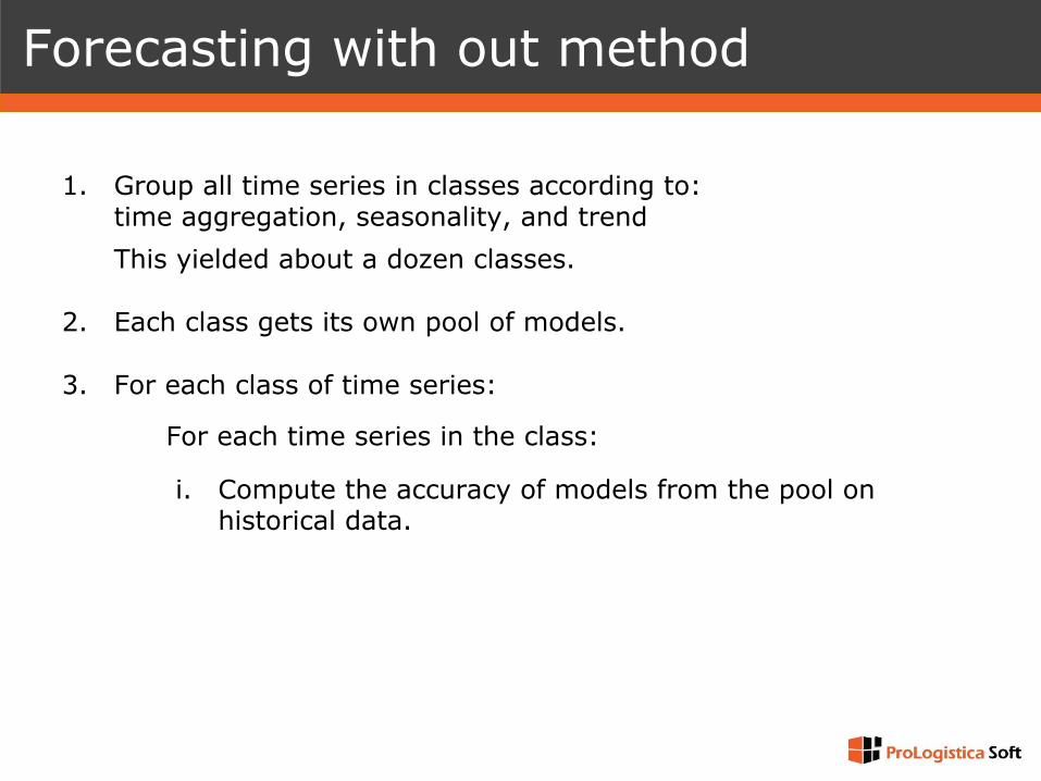
1. Group all time series in classes according to:time aggregation, seasonality, and trendThis yielded about a dozen classes.
2. Each class gets its own pool of models.
3. For each class of time series:
For each time series in the class:
i. Compute the accuracy of models from the pool on historical data.
ii. Assign a weight to each model based on the accuracy.
iii. Combine the models using their weights.
Forecasting with out method
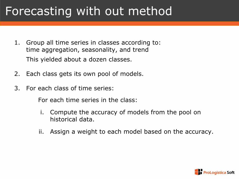
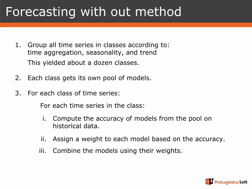
Historical accuracy
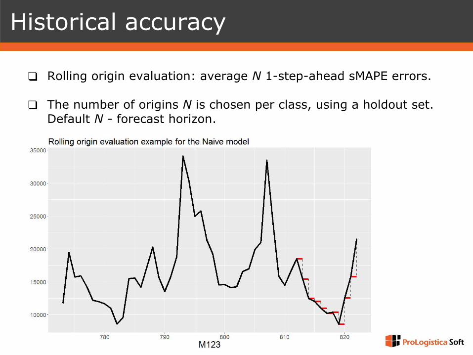
❑ Rolling origin evaluation: average N 1-step-ahead sMAPE errors.
❑ The number of origins N is chosen per class, using a holdout set. Default N - forecast horizon.
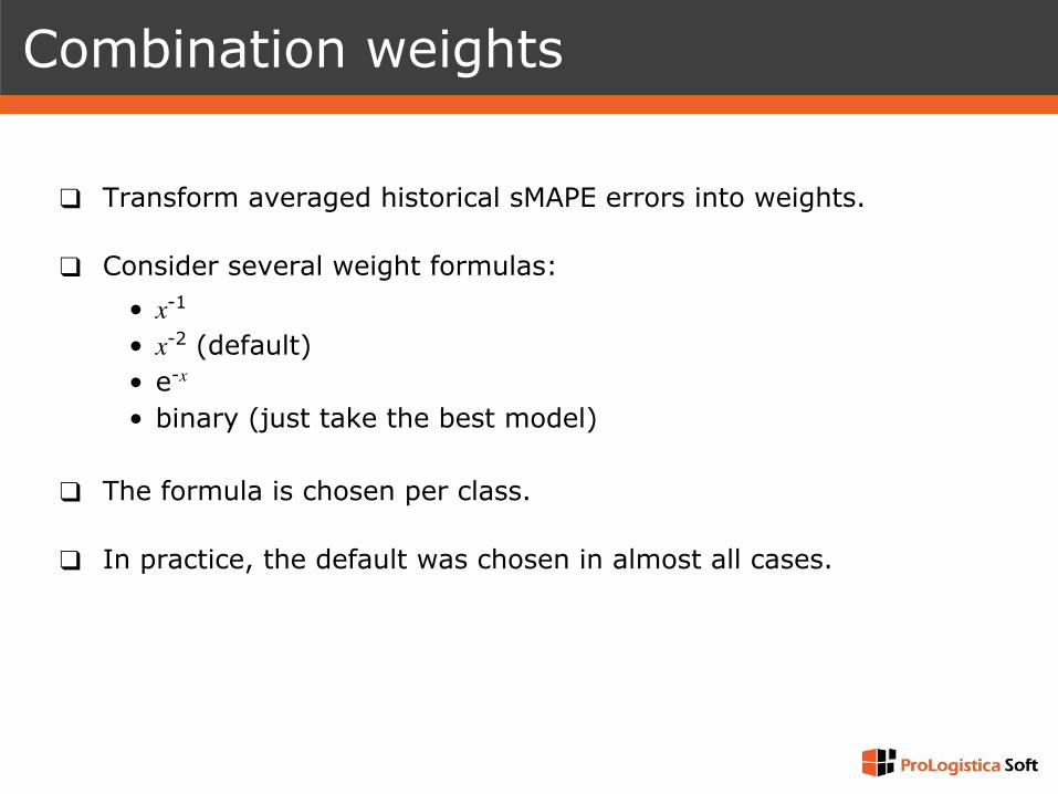
Combination weights
❑ Transform averaged historical sMAPE errors into weights.
❑ Consider several weight formulas:• 𝑥-1
• 𝑥-2 (default)• e-𝑥
• binary (just take the best model)
❑ The formula is chosen per class.
❑ In practice, the default was chosen in almost all cases.
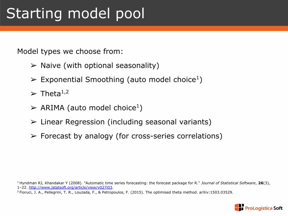
Model types we choose from:
➢ Naive (with optional seasonality)
➢ Exponential Smoothing (auto model choice1)
➢ Theta1,2
➢ ARIMA (auto model choice1)
➢ Linear Regression (including seasonal variants)
➢ Forecast by analogy (for cross-series correlations)
1 Hyndman RJ, Khandakar Y (2008). "Automatic time series forecasting: the forecast package for R." Journal of Statistical Software, 26(3), 1–22. http://www.jstatsoft.org/article/view/v027i03.2 Fioruci, J. A., Pellegrini, T. R., Louzada, F., & Petropoulos, F. (2015). The optimised theta method. arXiv:1503.03529.
Starting model pool

1. Start with a pool of all models, set other parameters to default.
2. For each time series in the class:
a. Split the series into training part and holdout partb. Sort all models by their holdout set error.c. Determine the combination weight for each model.
3. Combine all models. Compute the holdout set error.
4. In a loop, try removing models from the pool:
a. Remove the worst model.b. Put it back into the pool if the holdout set error of the
combined forecast increases.
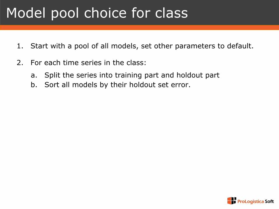
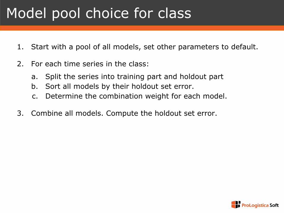
Model pool choice for class

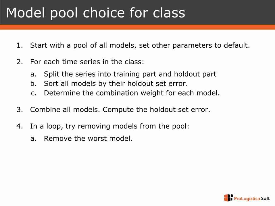
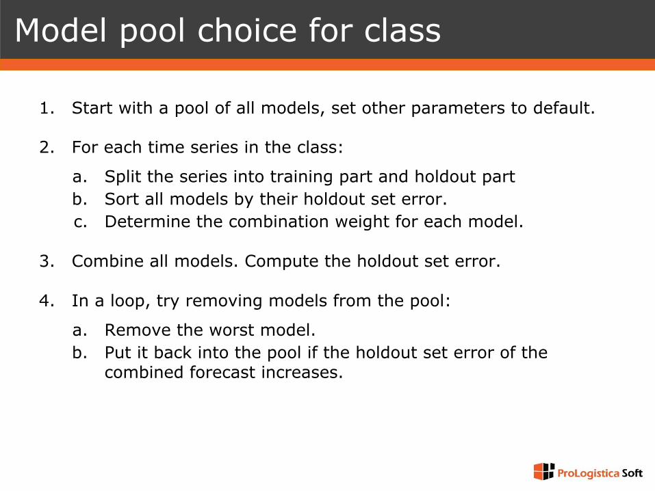
1. Start with a pool of all models, set other parameters to default.
2. For each time series in the class:
a. Split the series into training part and holdout partb. Sort all models by their holdout set error.c. Determine the combination weight for each model.
3. Combine all models. Compute the holdout set error.
4. In a loop, try removing models from the pool:
a. Remove the worst model.b. Put it back into the pool if the holdout set error of the
combined forecast increases.
Model pool choice for class

Model pool choice for class
1. Start with a pool of all models, set other parameters to default.
2. For each time series in the class:
a. Split the series into training part and holdout partb. Sort all models by their holdout set error.c. Determine the combination weight for each model.
3. Combine all models. Compute the holdout set error.
4. In a loop, try removing models from the pool:
a. Remove the worst model.b. Put it back into the pool if the holdout set error of the
combined forecast increases.
Model pool choice for class
1. Start with a pool of all models, set other parameters to default.
2. For each time series in the class:
a. Split the series into training part and holdout partb. Sort all models by their holdout set error.c. Determine the combination weight for each model.
3. Combine all models. Compute the holdout set error.
4. In a loop, try removing models from the pool:
a. Remove the worst model.b. Put it back into the pool if the holdout set error of the
combined forecast increases.
Model pool choice for class
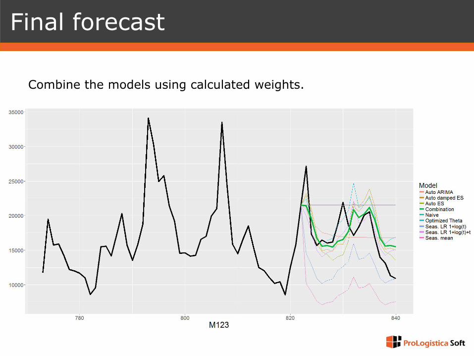
Final forecast
Combine the models using calculated weights.

Challenge: pool choice
Pool Model choice Final sMAPEFinal pool Combination 0.0769
Top 5 models Combination 0.0775
All models Combination 0.0777
Top 5 models Single model 0.0796
Final pool Single model 0.0798
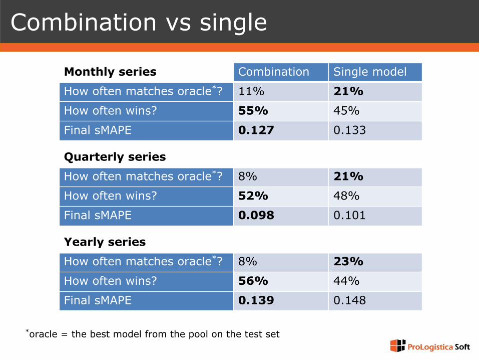
Combination vs single
Monthly series Combination Single model
How often matches oracle*? 11% 21%
How often wins? 55% 45%
Final sMAPE 0.127 0.133
Quarterly series
How often matches oracle*? 8% 21%
How often wins? 52% 48%
Final sMAPE 0.098 0.101
Yearly series
How often matches oracle*? 8% 23%
How often wins? 56% 44%
Final sMAPE 0.139 0.148
*oracle = the best model from the pool on the test set
❑ Core: combination of common statistical models, accuracy on historical data determines the weights.
❑ Simple yet effective!
❑ Main challenge: choosing the model pools.
Conclusions

PROLOGISTICA SOFT
Ostrowskiego 9, 53-238 Wrocław
Poland
phone: +48 71 716 44 65
e-mail: [email protected]
Read IJF preprint atarxiv.org/abs/1811.07761
Thank You
Maciej Pawlikowski+48 71 790 12 [email protected]
Agata Chorowska+48 695 860 [email protected]
❑ Better rolling origin evaluation parameters:
▪ forecast length (instead of a default 1)
▪ number of origins
❑ More fine-grained clustering, to allow for specialized model pools.
Possible improvements
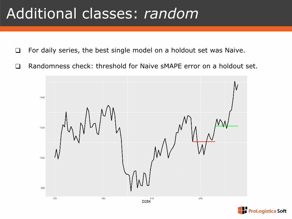
❑ For daily series, the best single model on a holdout set was Naive.
❑ Randomness check: threshold for Naive sMAPE error on a holdout set.
Additional classes: random
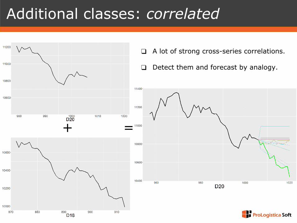
❑ A lot of strong cross-series correlations.
❑ Detect them and forecast by analogy.
Additional classes: correlated
+ =
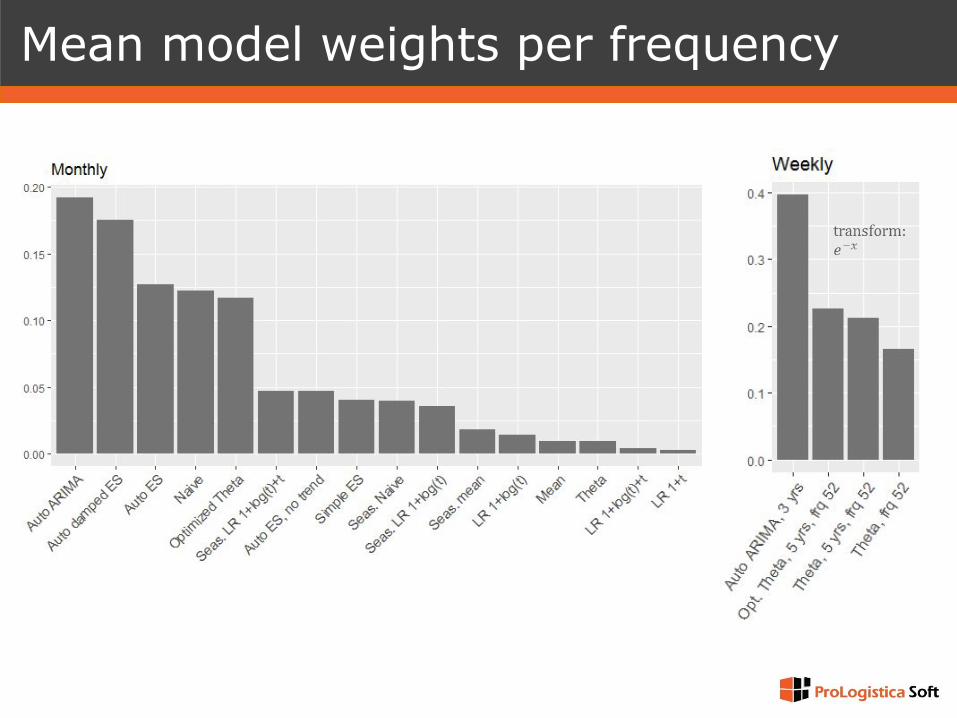
Mean model weights per frequency
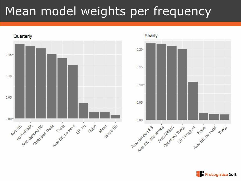
Mean model weights per frequency
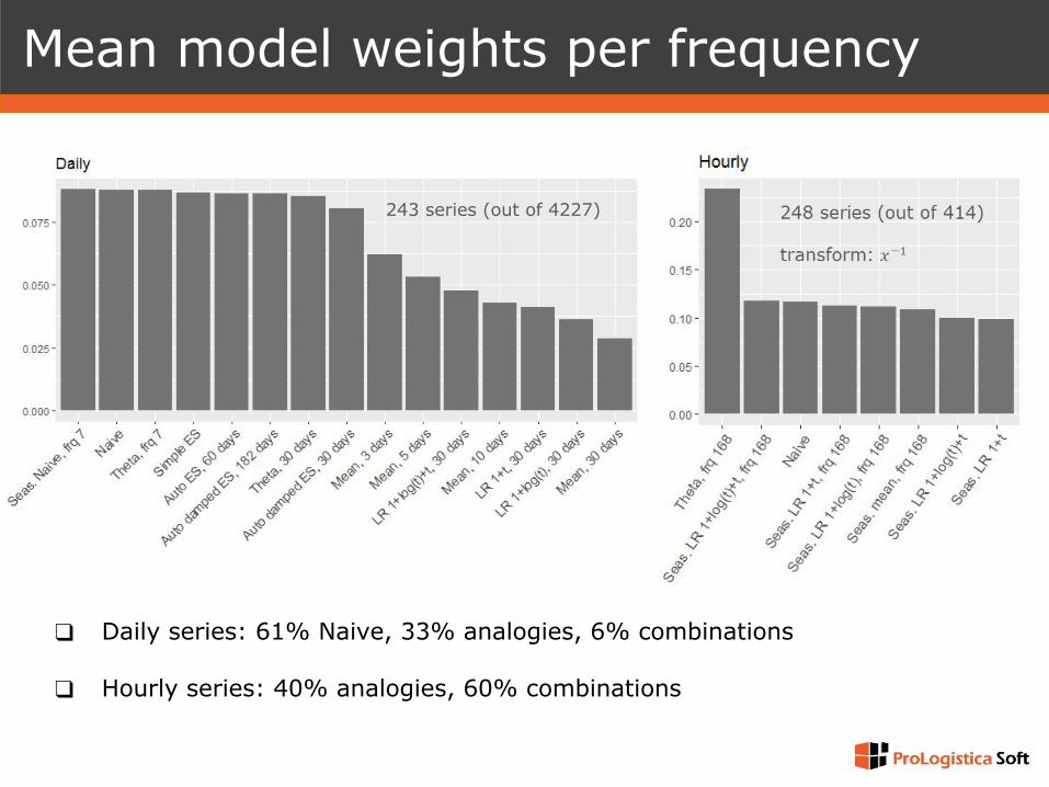
Mean model weights per frequency
❑ Daily series: 61% Naive, 33% analogies, 6% combinations
❑ Hourly series: 40% analogies, 60% combinations
243 series (out of 4227)