Embed Size (px)
Citation preview

Stat 302 Notes. Week 9, Hour 3, Page 1 / 39
Week 9 Hour 3
Stepwise method
Modern Model Selection Methods
Quantile-Quantile plot and tests for normality

Stat 302 Notes. Week 9, Hour 3, Page 2 / 39
Stepwise
Now that we've introduced interactions, there are so many
options for building statistical models that we need a method
to work through many possibilities quickly.
The stepwise method is one such method.

Stat 302 Notes. Week 9, Hour 3, Page 3 / 39
For the stepwise method, you need..
- One response variable
- A list of explanatory variables that could included in the
model.
- A criterion for evaluating the quality of a model.
Ideally, stepwise will find the combination of those
explanatory variables that produces a model that gets the best
score for the selected criterion.

Stat 302 Notes. Week 9, Hour 3, Page 4 / 39
The most popular R function for stepwise is stepAIC() in the
MASS package.
The default criterion used is AIC, but it’s easy to change it to
BIC or R-squared*.
stepAIC inputs a ‘starting model’, which includes all the terms
you want to consider. It outputs a ‘final model’ which you can
use just like anything you would get from lm()
*Don’t use R-squared. Seriously. Just don’t.

Stat 302 Notes. Week 9, Hour 3, Page 5 / 39
Consider the gapminder dataset, and our model of birth rates
from before.
When we found the best model using VIF, and again with AIC,
we didn’t consider interactions.
For the six variables (all continuous) we were considering
before, there are 5+4+3+2+1=15 possible interaction terms to
consider.
We won’t consider any polynomial terms.
Stat 302 Notes. Week 9, Hour 3, Page 6 / 39
For each term, we can either include it or not, independently
of the other terms included.
That means there are 221, or ~2 million possible models we can
build using the 6 main effects and 15 interactions.
Rather than trying to manually find the best combination, we
can feed this information into a stepwise function in R and it
will find one for us.

Stat 302 Notes. Week 9, Hour 3, Page 7 / 39
Let’s try it:
Input

Stat 302 Notes. Week 9, Hour 3, Page 8 / 39
Summary of output:
14 of 21 possible terms have been included.

Stat 302 Notes. Week 9, Hour 3, Page 9 / 39
A 14-term regression may work for some situations, but we
may also want a simpler model. That is, one with fewer terms.
To do this, we need to use a criterion with a larger penalty for
complexity, such as the Bayesian Information Criterion (BIC).
To use this we change the ‘k’ setting in stepAIC, which is
penalty per term. The default value for ‘k’ is 2.

Stat 302 Notes. Week 9, Hour 3, Page 10 / 39
BIC-based output:
13 of 21 possible terms have been included.

Stat 302 Notes. Week 9, Hour 3, Page 11 / 39
Three big drawbacks to the stepwise method:
1. It can only consider terms that you specify. It won’t try
things like additional polynomial terms, interactions, or
transformations for you.
2. It doesn’t actually try every possible candidate model, so
there is a chance that a better model exists that the stepwise
method will miss.

Stat 302 Notes. Week 9, Hour 3, Page 12 / 39
3. It blindly applies the given criterion without regards to other
concerns like non-linear fits, and influential outliers, co-
linearity.
In short, the stepwise method is…
not a replacement for human judgement.

Stat 302 Notes. Week 9, Hour 3, Page 13 / 39
How do these steps work?
Stat 302 Notes. Week 9, Hour 3, Page 14 / 39
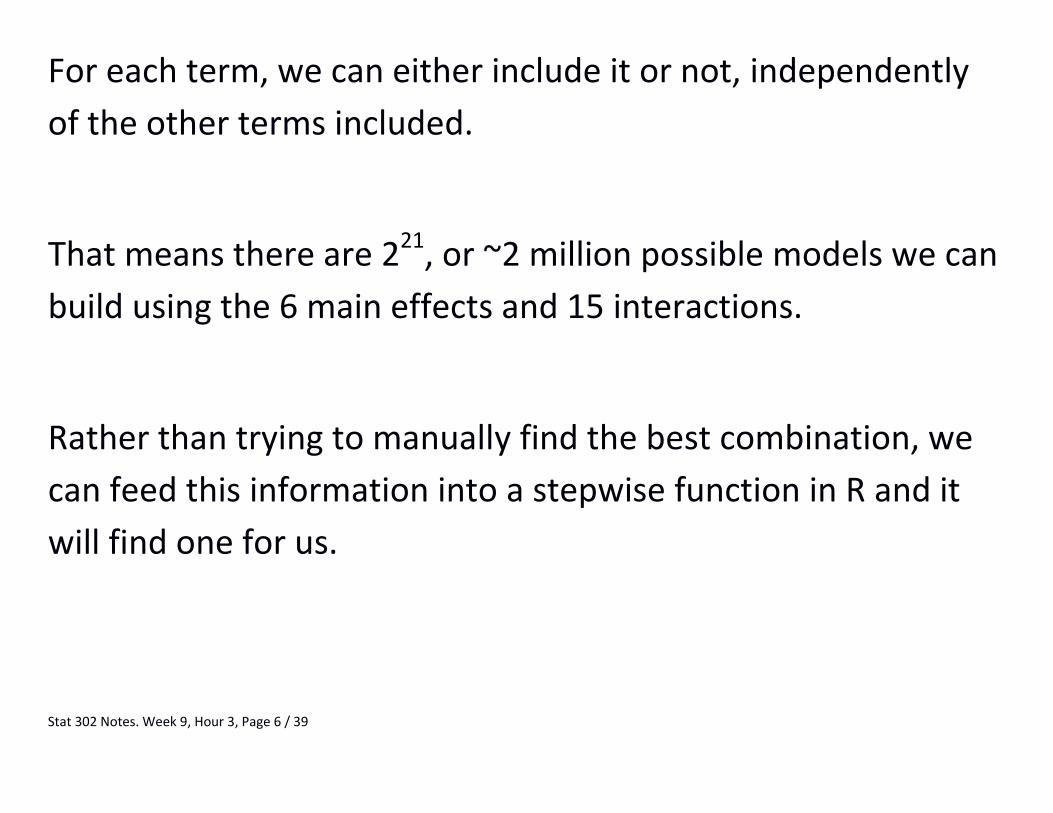
Stepwise mechanics Stepwise ‘searches’ for the best regression by repeating the
following steps:
1. Get the AIC (or other criterion) for the <current model>.
2. For each of the terms you can add (given in a list*), add that
term to <current model> . Get the AIC for each ‘add 1’ model.

Stat 302 Notes. Week 9, Hour 3, Page 15 / 39
3. For each of the terms you can remove (anything in the
model that doesn’t violate heredity and hierarchy*), remove
that term. Get the AIC for each ‘drop 1’ model.
4. Select the model with the best AIC and make that the new
<current model>.
5. If the new <current model> is the same as the old one, we
are done.
Otherwise, return to Step 1.

Stat 302 Notes. Week 9, Hour 3, Page 16 / 39
*About Step 2: You don’t have to start with a ‘full model’ that
has every term you might consider. It’s just one way to specify
a ‘starting point’ for the stepwise method.
We could also…
… start from a null model (one without ANY terms) and add
them in one at a time.
… start with some human-made model, and let the system add
or remove terms to find a better one.

Stat 302 Notes. Week 9, Hour 3, Page 17 / 39
The starting point matters because of local optima.
Global optimum: The best of all possibilities.
Local optimum: The best of all NEARBY possibilities.

Stat 302 Notes. Week 9, Hour 3, Page 18 / 39
If a model has a better AIC than any term ‘near it’ (e.g. being
different by only one-term), then the stepwise method could
select this ‘locally best’ model, even if a better one exists.

Stat 302 Notes. Week 9, Hour 3, Page 19 / 39
*About Step 3:
If a variable shows up in more than one term in a model, then
the stepwise method (at least in R) will not consider removing
a simple term if a more complex term with the sample variable
is still in it.
For example:
Stepwise won’t remove a term for ‘wind’ from the model if
there is also a term for ‘wind2’ or a ‘wind:solar’ interaction in it
too.

Stat 302 Notes. Week 9, Hour 3, Page 20 / 39
Model selection in general
Stepwise isn’t the only method of model selection. It’s not
even the best method available. It just happens to be one of
the simplest.
(The following few slides are mostly for your future work with
data. They won’t be on the midterm or final.)
Other methods you may want to consider are…

Stat 302 Notes. Week 9, Hour 3, Page 21 / 39
All-Subsets Method:
Similar to the stepwise method in that it selects a set of
regression terms that gives you the best value for AIC (or some
other criterion of choice).
Unlike stepwise, all-subsets considers every possible
combination of the given regression terms. So the problem of
hitting a ‘local optimum’ is solved.
However, checking every method can be much slower, and
really not worth the extra effort.

Stat 302 Notes. Week 9, Hour 3, Page 22 / 39
Regression trees: Tree methods model a response as coming
from a collection of binary decisions.
Dummies, interactions, and polynomial terms work fine, and
the response can be categorical or numeric.

Stat 302 Notes. Week 9, Hour 3, Page 23 / 39
LASSO:
A LASSO model is a regression model with one tradeoff:
The LASSO sets non-significant terms to zero, rather than some
random near-zero amount. This makes the model much easier
to interpret and read, but at the cost of larger errors (i.e.
worse R-squared, AIC).
The LASSO is also adjustable by deciding how significant a term
has to be to avoid being set to zero.
It suitable for situations with MANY explanatory variables.

Stat 302 Notes. Week 9, Hour 3, Page 24 / 39
Automatic model selection: Avoiding work like never before!

Stat 302 Notes. Week 9, Hour 3, Page 25 / 39
Diagnostics for Normality
Stepwise (and other model selection methods) will determine
the ‘best’ model according to a single criterion.
A single criterion isn’t sufficient to cover all the aspects of the
model.
We need ways to check for problems like uneven variance,
influential outliers, and non-normality.
The residuals reveal these problems.
Stat 302 Notes. Week 9, Hour 3, Page 26 / 39
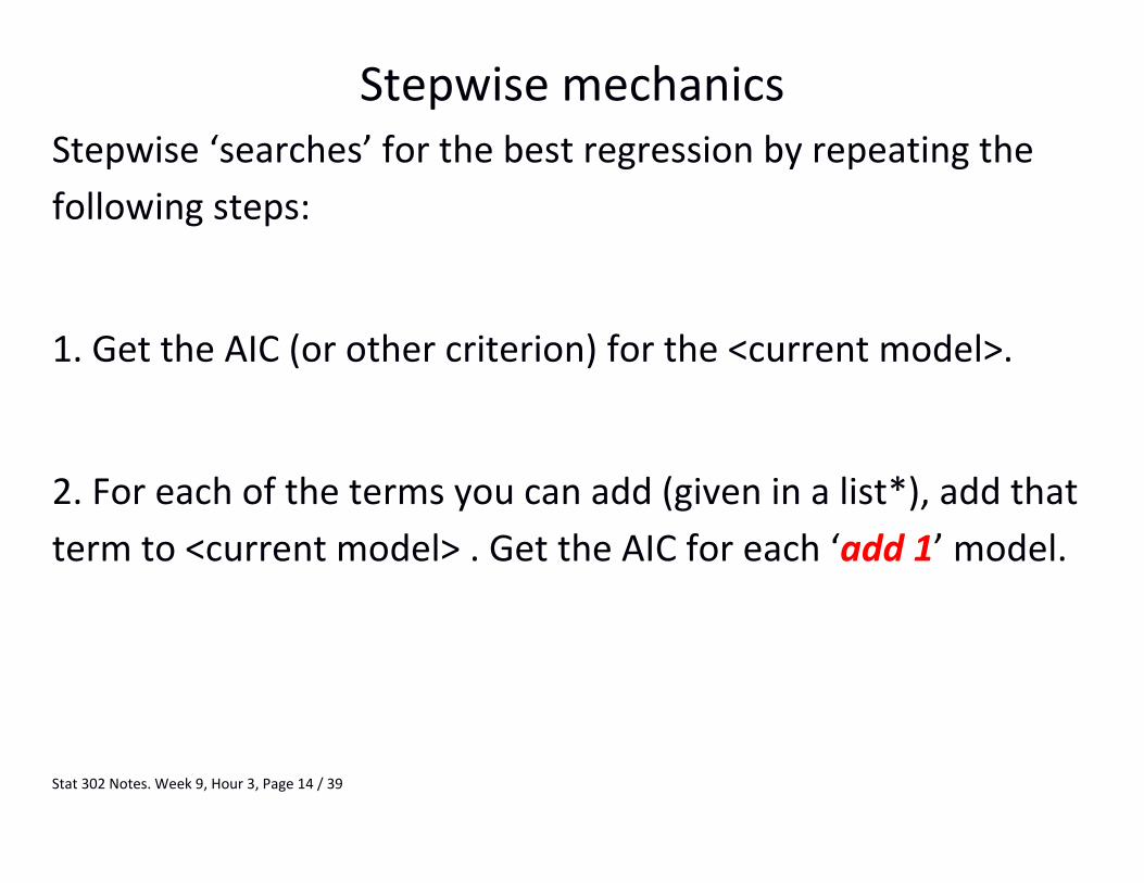
A quantile-quantile plot tests normality. A straight line Q-Q
plot is normal or close to normal.
The dotted lines are confidence bands where we’re 95% sure a
Q-Q plot would go IF the distribution was normal.

Stat 302 Notes. Week 9, Hour 3, Page 27 / 39
Outliers or distributions that have more variance than a
normal distribution will have a Q-Q plot that curves at the end.

Stat 302 Notes. Week 9, Hour 3, Page 28 / 39
Skewed distribution are non-normal. They show up as a single
bend on a Q-Q plot.

Stat 302 Notes. Week 9, Hour 3, Page 29 / 39
Bimodal distributions will look even worse – the Q-Q plot will
not only bend, but ‘jump’ somewhere between the modes.

Stat 302 Notes. Week 9, Hour 3, Page 30 / 39
Compared to histograms, Q-Q plots have two big advantages.
1. Q-Q plots are more formal. They can be overlaid with
confidence bands of a selected level (95% by default).
This allows you to test the null hypothesis of normality, and
see where that hypothesis would be rejected.
Interpretations are a lot less open to interpretation. It’s clear
when a distribution is or isn’t normal.
You can even test against other distributions if you wish!

Stat 302 Notes. Week 9, Hour 3, Page 31 / 39
2. Q-Q plots are more sensitive.
In the above examples, the deviations from normality are
blatant and obvious.
Usually, these deviations are more subtle and can’t be pointed
out so easily by a histogram. A Q-Q plot, however, is much
more likely to show these issues.

Stat 302 Notes. Week 9, Hour 3, Page 32 / 39
Consider this set of values with uneven variance.
The histogram looks very much like it would with a normal.
.

Stat 302 Notes. Week 9, Hour 3, Page 33 / 39
Now look at the QQ-plot. The values appear mostly on the line,
but the confidence bands go crazy. (Extremely wide at the
extremes, and extremely thin in the middle)

Stat 302 Notes. Week 9, Hour 3, Page 34 / 39
Q-Q Plots help you handle lots of terms together.

Stat 302 Notes. Week 9, Hour 3, Page 35 / 39
Shapiro-Wilks Test
The Shapiro test is a hypothesis test for normality.
It works like other tests the Kruskal-Wallis and the Bartlett
tests for equal variance.
Your null hypothesis is the no-problem scenario. In the Shapiro
test’s case, this is ‘your data is normally distributed’.
- If the p-value is large, there is no evidence against normality.
- If the p-value is small, you have evidence of non-normality.
Stat 302 Notes. Week 9, Hour 3, Page 36 / 39
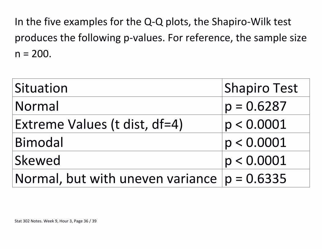
In the five examples for the Q-Q plots, the Shapiro-Wilk test
produces the following p-values. For reference, the sample size
n = 200.
Situation Shapiro Test Normal p = 0.6287 Extreme Values (t dist, df=4) p < 0.0001 Bimodal p < 0.0001 Skewed p < 0.0001 Normal, but with uneven variance p = 0.6335

Stat 302 Notes. Week 9, Hour 3, Page 37 / 39
Like other hypothesis tests, sample size matters.
- The Shapiro test will be unable to find most non-normality in
a small sample.
Skewed Distribution Shapiro Test N = 10 p = 0.2331 N = 20 p = 0.0128 N = 30 p = 0.0008 N = 50 p < 0.0001 N = 200 p < 0.0001
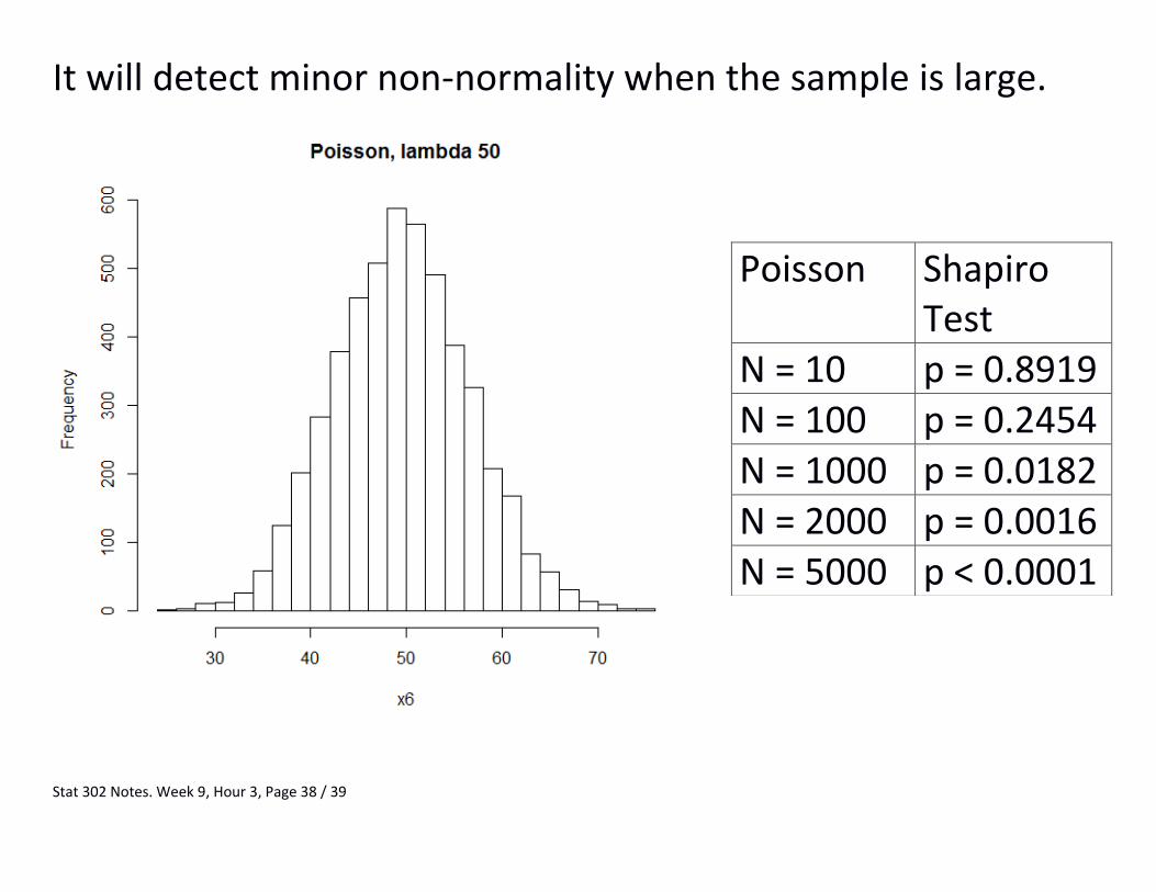
Stat 302 Notes. Week 9, Hour 3, Page 38 / 39
It will detect minor non-normality when the sample is large.
Poisson Shapiro Test
N = 10 p = 0.8919 N = 100 p = 0.2454 N = 1000 p = 0.0182 N = 2000 p = 0.0016 N = 5000 p < 0.0001

Stat 302 Notes. Week 9, Hour 3, Page 39 / 39
Next week:
Cross-Validation
Missing data
Imputation (end of Midterm 2 material)