Week 4: Simple Linear Regression III

Week 4: Simple Linear Regression III

Marcelo Coca Perraillon

University of ColoradoAnschutz Medical Campus

Health Services Research Methods IHSMP 7607

2019

These slides are part of a forthcoming book to be published by CambridgeUniversity Press. For more information, go to perraillon.com/PLH. c©Thismaterial is copyrighted. Please see the entire copyright notice on the book’swebsite.

Updated notes are here: https://clas.ucdenver.edu/marcelo-perraillon/

teaching/health-services-research-methods-i-hsmp-76071

perraillon.com/PLH

https://clas.ucdenver.edu/marcelo-perraillon/teaching/health-services-research-methods-i-hsmp-7607

https://clas.ucdenver.edu/marcelo-perraillon/teaching/health-services-research-methods-i-hsmp-7607

Outline

Goodness of fit

Confidence intervals

Loose ends

2

Partitioning variance

Recall from last class that we saw that the sum of the residual is zero,which implies that the predicted ¯y is the same as the observed y , soalways ¯y = y

Also, for each observation i in our dataset the following is always trueby definition of the residual:

yi = yi + εi , which is equivalent to

yi = yi + (yi − yi )

In words, an observed outcome value yi is equal to its predicted valueplus the residual

We can do a little bit of algebra to go from this equality to somethingmore interesting about the way we can interpret linear regression

3


Subtract y from both sides of the equation and group terms:

(yi − y) = (yi − y) + (yi − yi )

Since y = ¯y :

(yi − y) = (yi − ¯y) + (yi − yi )

Stare at the last equation for a while. Looks familiar?

Deviation from mean observed outcome = Deviation from fit forpredicted values + Model residual

The above equality can be expressed in terms of the sum of squares;the proof is messy. Your textbook skips several steps; see WooldridgeChapter 2

4


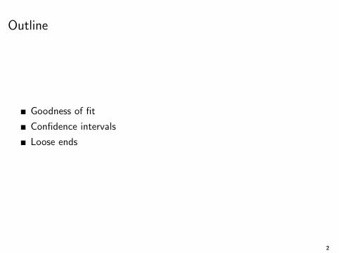
We need to define the following terms

Total sum of squared deviations: SST =∑n

i=1(yi − y)2

Sum of squares due to the regression: SSR =∑n

i=1(yi − ¯y)2

Sum of squared residuals (errors): SSE =∑n

i=1(yi − y)2

We can then write (yi − y) = (yi − ¯y) + (yi − yi ) as

SST = SSR + SSE

SST/(n-1) is the sample variance of the outcome y

SSR/(n-1) is the sample variance of the predicted values y

SSE/(n-1) is the sample variance of the residuals (but really, dividedby n − 2)

Confusion alert: in SSR, “R” stands for regression. In SSE, E standsfor error, even though it should be “residual,” not errors. Wooldridgeuses SSE for ”explained” or regression. And then Stata uses otherlabels...

5


SST = SSR + SSE is telling us that the observed variance of theoutcome was partitioned into two parts, one that is explained by ourmodel (SSR) and another that our model cannot explain (SSE)

So we could then measure how good our model is by the ratio SSRSST

(goodness of fit)

In other words, the fraction of the total observed variance of theoutcome that is explained by our model. That’s the famous R2:

R2 = SSRSST = 1 − SSE

SST

Another way: total observed variance = explained variance +unexplained variance

6

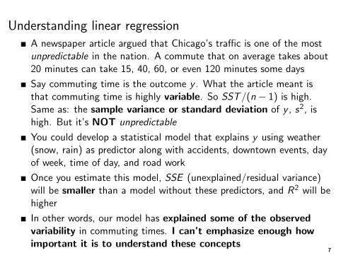
Understanding linear regressionA newspaper article argued that Chicago’s traffic is one of the mostunpredictable in the nation. A commute that on average takes about20 minutes can take 15, 40, 60, or even 120 minutes some days

Say commuting time is the outcome y . What the article meant isthat commuting time is highly variable. So SST/(n − 1) is high.Same as: the sample variance or standard deviation of y , s2, ishigh. But it’s NOT unpredictable

You could develop a statistical model that explains y using weather(snow, rain) as predictor along with accidents, downtown events, dayof week, time of day, and road work

Once you estimate this model, SSE (unexplained/residual variance)will be smaller than a model without these predictors, and R2 will behigher

In other words, our model has explained some of the observedvariability in commuting times. I can’t emphasize enough howimportant it is to understand these concepts

7

Calculate using Stata

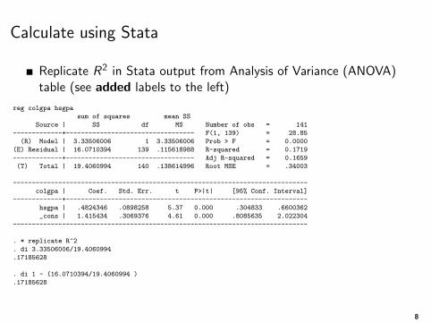
Replicate R2 in Stata output from Analysis of Variance (ANOVA)table (see added labels to the left)

reg colgpa hsgpa

sum of squares mean SS

Source | SS df MS Number of obs = 141

-------------+---------------------------------- F(1, 139) = 28.85

(R) Model | 3.33506006 1 3.33506006 Prob > F = 0.0000

(E) Residual | 16.0710394 139 .115618988 R-squared = 0.1719

-------------+---------------------------------- Adj R-squared = 0.1659

(T) Total | 19.4060994 140 .138614996 Root MSE = .34003

------------------------------------------------------------------------------

colgpa | Coef. Std. Err. t P>|t| [95% Conf. Interval]

-------------+----------------------------------------------------------------

hsgpa | .4824346 .0898258 5.37 0.000 .304833 .6600362

_cons | 1.415434 .3069376 4.61 0.000 .8085635 2.022304

------------------------------------------------------------------------------

. * replicate R^2

. di 3.33506006/19.4060994

.17185628

. di 1 - (16.0710394/19.4060994 )

.17185628

8

Calculate using Stata

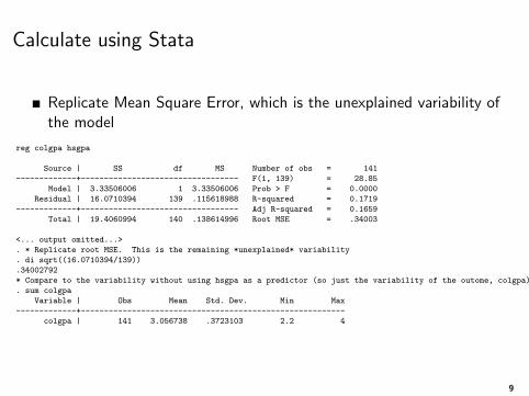
Replicate Mean Square Error, which is the unexplained variability ofthe model

reg colgpa hsgpa


-------------+---------------------------------- F(1, 139) = 28.85

Model | 3.33506006 1 3.33506006 Prob > F = 0.0000

Residual | 16.0710394 139 .115618988 R-squared = 0.1719

-------------+---------------------------------- Adj R-squared = 0.1659

Total | 19.4060994 140 .138614996 Root MSE = .34003

<... output omitted...>

. * Replicate root MSE. This is the remaining *unexplained* variability

. di sqrt((16.0710394/139))

.34002792

* Compare to the variability without using hsgpa as a predictor (so just the variability of the outome, colgpa)

. sum colgpa

Variable | Obs Mean Std. Dev. Min Max

-------------+---------------------------------------------------------

colgpa | 141 3.056738 .3723103 2.2 4

9

We can go from explained and unexplained standarddeviation to R2

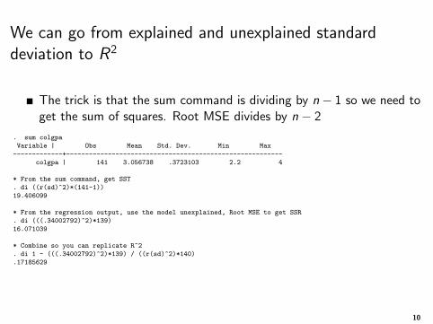
The trick is that the sum command is dividing by n− 1 so we need toget the sum of squares. Root MSE divides by n − 2

. sum colgpa


-------------+---------------------------------------------------------

colgpa | 141 3.056738 .3723103 2.2 4

* From the sum command, get SST

. di ((r(sd)^2)*(141-1))

19.406099

* From the regression output, use the model unexplained, Root MSE to get SSR

. di (((.34002792)^2)*139)

16.071039

* Combine so you can replicate R^2

. di 1 - (((.34002792)^2)*139) / ((r(sd)^2)*140)

.17185629

10

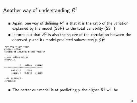
Another way of understanding R2

Again, one way of defining R2 is that it is the ratio of the variationexplained by the model (SSR) to the total variability (SST)

It turns out that R2 is also the square of the correlation between theobserved y and its model-predicted values: cor(y , y)2

qui reg colgpa hsgpa

predict colhat

(option xb assumed; fitted values)

. corr colhat colgpa

(obs=141)

| colhat colgpa

-------------+------------------

colhat | 1.0000

colgpa | 0.4146 1.0000

. di 0.4146^2

.17189316

The better our model is at predicting y the higher R2 will be

11

Confidence Intervals

We want to build a confidence interval for β

The proper interpretation of a confidence interval in the frequentistapproach is that if we repeated the experiment many times, about x%percent of the time the value of β would be within the confidenceinterval

By convention, we build 95% confidence intervals, which impliesα = 0.05

Intuitively, we need to know the distribution of β and its precision,the standard error. To derive these, we need to assume ε distributesN(0, σ2) iid

A formula for the confidence interval of βi is:

βi ± t(n−2,α/2)se(βi )

We saw that t(n−2,α/2) in the context of Wald tests. In the normal,it’s 1.98

12

Confidence Intervals

We use t-student but remember that when n is large (larger thanabout 120) the t distribution approximates a normal distribution

Recall this graph from stats 101 and Wikipedia :

13

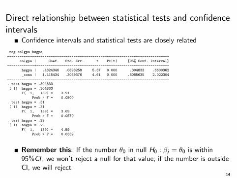
Direct relationship between statistical tests and confidenceintervals

Confidence intervals and statistical tests are closely related

reg colgpa hsgpa

------------------------------------------------------------------------------


-------------+----------------------------------------------------------------

hsgpa | .4824346 .0898258 5.37 0.000 .304833 .6600362

_cons | 1.415434 .3069376 4.61 0.000 .8085635 2.022304

------------------------------------------------------------------------------

. test hsgpa = .304833

( 1) hsgpa = .304833

F( 1, 139) = 3.91

Prob > F = 0.0500

. test hsgpa = .31

( 1) hsgpa = .31

F( 1, 139) = 3.69

Prob > F = 0.0570

. test hsgpa = .29

( 1) hsgpa = .29

F( 1, 139) = 4.59

Prob > F = 0.0339

Remember this: If the number θ0 in null H0 : βj = θ0 is within95%CI , we won’t reject a null for that value; if the number is outsideCI, we will reject

14

As usual, simulations are awesome

* simulate 9000 observations

set obs 9000

gen betahsgpa = rnormal(.4824346,.0898258)

sum


-------------+---------------------------------------------------------

betahsgpa | 9,000 .4826007 .0900429 .1583372 .9124259

* count the number of times beta is within the confidence interval

count if betahsgpa >= .304833 & betahsgpa <= .6600362

8,552

di 8552/9000

.95022222

* Do the same with a t-student

. gen zt = rt(139)

. * By default, Stata simulate a standard t, mean zero and sd of 1

sum zt


-------------+---------------------------------------------------------

zt | 9,000 .0019048 .9972998 -3.567863 3.574553

. * Need to retransform

gen betat = .0898258*zt + .4824346

sum betat


-------------+---------------------------------------------------------

betat | 9,000 .4826057 .0895833 .1619485 .8035216

count if betat >= .304833 & betat <= .6600362

8,576

. di 8576/9000

.95288889

15

What just happened?

We estimated a parameter β and its standard error√var(β)

Because of assumptions about ε distributing N(0, σ2) we know thatasymptotically β distributes normal (but the Wald test distributest-student)

That’s all we need to calculate confidence intervals and hypothesestests about the true β in the population

Recall that a probability distribution function describes the values arandom variable can take and the probability of those values. So wecan make statements about the probability of the parameter takingcertain values or being within an interval if we know the distributionof the parameter

We also know that the t-student converges to a normal for sampleslarger than about 120, so we could just use the normal distribution

16

Distributions

Note the slightly fatter tails of the t-student

17

We can do more

Other confidence intervals?centile betahsgpa, centile(2.5(5)97.5)

-- Binom. Interp. --

Variable | Obs Percentile Centile [95% Conf. Interval]

-------------+-------------------------------------------------------------

betahsgpa | 9,000 2.5 .3028123 .2985525 .3087895

| 7.5 .3527713 .3494937 .3565182

| 12.5 .3789864 .375991 .3828722

| 17.5 .3990816 .3966145 .4013201

| 22.5 .4146384 .4117871 .4172412

| 27.5 .428773 .4263326 .4314667

| 32.5 .4425001 .440095 .4447364

| 37.5 .4546066 .4523425 .4566871

| 42.5 .466314 .4637115 .4679226

| 47.5 .4773481 .4747118 .4795888

| 52.5 .4890074 .486511 .4909871

| 57.5 .4991535 .4969174 .5015363

| 62.5 .5109765 .5086741 .5133994

| 67.5 .5230142 .5210292 .5253365

| 72.5 .5359863 .5334756 .5384137

| 77.5 .5504502 .5473233 .5534496

| 82.5 .5673794 .5640415 .5700424

| 87.5 .5862278 .5831443 .589366

| 92.5 .6109914 .6076231 .6150107

| 97.5 .6565534 .6518573 .6633566

Note how close the 2.5 and 97.5 percentiles follow the reg CI above

18

Even more

What is the probability that the coefficient for hsgpa is greater than0.4? Greater than 0.8?. count if betahsgpa >0.4

7,394

. di 7394/9000

.81822222

count if betahsgpa >0.8

2

di 2/9000

.00022222

Fairly likely and fairly unlikely, respectively (look at distribution)

We have no evidence that the coefficient will be remotely close tozero so no surprise about the p-value in the regression output

Caution: We only have one predictor/covariate here. With more,there is a correlation between βj . They distribute multivariate normalwith a variance-covariance matrix. We will see examples

19

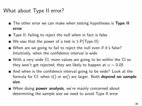
What about Type II error?

The other error we can make when testing hypotheses is Type IIerror

Type II: failing to reject the null when in fact is false

We saw that the power of a test is 1-P(Type II)

When are we going to fail to reject the null even if it’s false?Intuitively, when the confidence interval is wide

With a very wide CI, more values are going to be within the CI sothey won’t get rejected; they are likely to happen at α = 0.05

And when is the confidence interval going to be wide? Look at theformula for CI: when t() or se() are larger. Both depend on samplesize

When doing power analysis, we’re mainly concerned aboutdetermining the sample size we need to avoid Type II error

20

Loose ends

We have only one thing left to explain and replicate from theregression output. What is that F test?In the grades example:


-------------+---------------------------------- F(1, 139) = 28.85

Model | 3.33506006 1 3.33506006 Prob > F = 0.0000


-------------+---------------------------------- Adj R-squared = 0.1659

Total | 19.4060994 140 .138614996 Root MSE = .34003

That’s a test of the overall validity of the model. The null is thatβ1 = ... = βj = 0. Here, only one, so Ho : β1 = 0

It’s the ratio MSR/MSE = 3.33506006/.115618988 = 28.845263 (soregression/model to residual). As you know by now, it is F because itis the ratio of two chi-squares

Once we cover maximum likelihood we we will see another moregeneral approach to compare models, the likelihood ratio test

Both test are (asymptotically) equivalent

21

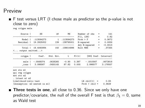
Preview

F test versus LRT (I chose male as predictor so the p-value is notclose to zero)reg colgpa male


-------------+---------------------------------- F(1, 139) = 0.82

Model | .113594273 1 .113594273 Prob > F = 0.3672


-------------+---------------------------------- Adj R-squared = -0.0013

Total | 19.4060994 140 .138614996 Root MSE = .37255

<... output omitted...>

------------------------------------------------------------------------------


-------------+----------------------------------------------------------------

male | -.0568374 .0628265 -0.90 0.367 -.1810567 .0673818

_cons | 3.086567 .0455145 67.82 0.000 2.996577 3.176557

------------------------------------------------------------------------------

est sto m1

qui reg colgpa

est sto m2

. lrtest m1 m2

Likelihood-ratio test LR chi2(1) = 0.83

(Assumption: m2 nested in m1) Prob > chi2 = 0.3629

Three tests in one, all close to 0.36. Since we only have onepredictor/covariate, the null of the overall F test is that β1 = 0, sameas Wald test

22

Summary

Linear regression can be thought of as partitioning the variance intotwo components, explained and unexplained

We can measure the goodness of fit of a model based on thecomparison of these variances

Be carefully about the context. We are talking about a linearmodel with ε N(0, σ2) and iid

Not the same in other type of models but the main ideas are valid

Once we know the asymptotic distribution of a parameter and itsstandard deviation (i.e. standar error) we have all we need to testhypotheses and build CIs

23

Documents

Week 4: Simple Linear Regression III