Week 4: History / philosophy, distance methodsevolution.gs.washington.edu/gs570/2010/week4.pdf · Week 4: History / philosophy, distance methods – p.5/73 Reptiles and ﬁshes are

Week 4: History / philosophy, distance methods

Genome 570

January, 2010

Week 4: History / philosophy, distance methods – p.1/73

Ernst Mayr and George Gaylord Simpson

Ernst Mayr (1905-2005) George Gaylord Simpson (1902-1984)


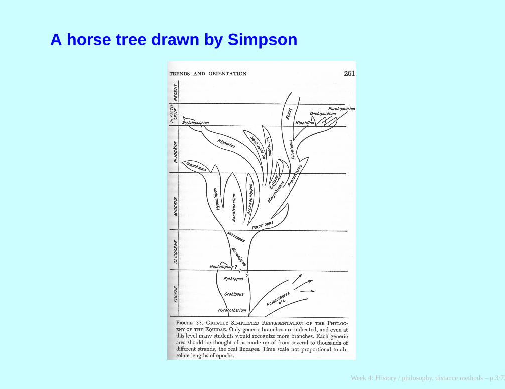
A horse tree drawn by Simpson


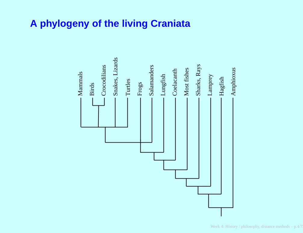
A phylogeny of the living Craniata

Mam

mal

s

Bird

s

Cro

codi

lians

Sna

kes,

Liz

ards

Tur

tles

Fro

gs

Sal

aman

ders

Lung

fish

Coe

laca

nth

Sha

rks,

Ray

s

Lam

prey

Hag

fish

Am

phio

xus

Mos

t fis

hes


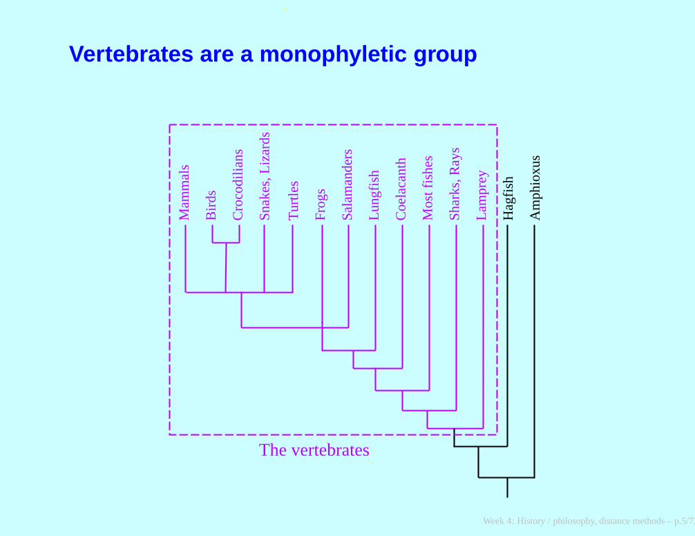
Vertebrates are a monophyletic group

Mam

mal

s

Bird

s

Cro

codi

lians

Sna

kes,

Liz

ards

Tur

tles

Fro

gs

Sal

aman

ders

Lung

fish

Coe

laca

nth

Sha

rks,

Ray

s

Lam

prey

Hag

fish

Am

phio

xus

The vertebratesM

ost f

ishe

s


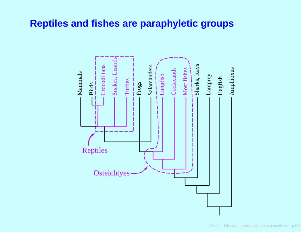
Reptiles and fishes are paraphyletic groups

Mam

mal

s

Bird

s

Cro

codi

lians

Sna

kes,

Liz

ards

Tur

tles

Fro

gs

Sal

aman

ders

Lung

fish

Coe

laca

nth

Sha

rks,

Ray

s

Lam

prey

Hag

fish

Am

phio

xus

Osteichtyes

Reptiles

Mos

t fis

hes


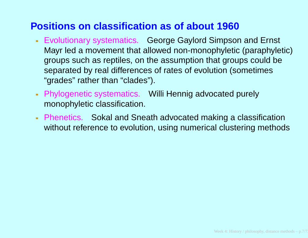
Positions on classification as of about 1960Evolutionary systematics. George Gaylord Simpson and ErnstMayr led a movement that allowed non-monophyletic (paraphyletic)groups such as reptiles, on the assumption that groups could beseparated by real differences of rates of evolution (sometimes“grades” rather than “clades”).

Phylogenetic systematics. Willi Hennig advocated purelymonophyletic classification.

Phenetics. Sokal and Sneath advocated making a classificationwithout reference to evolution, using numerical clustering methods


Peter Sneath in 1962 and Robert Sokal in 1964


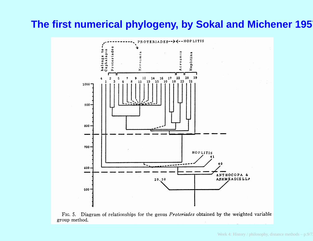
The first numerical phylogeny, by Sokal and Michener 1957


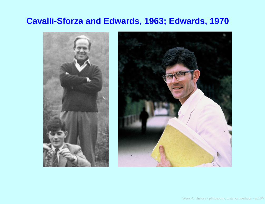
Cavalli-Sforza and Edwards, 1963; Edwards, 1970


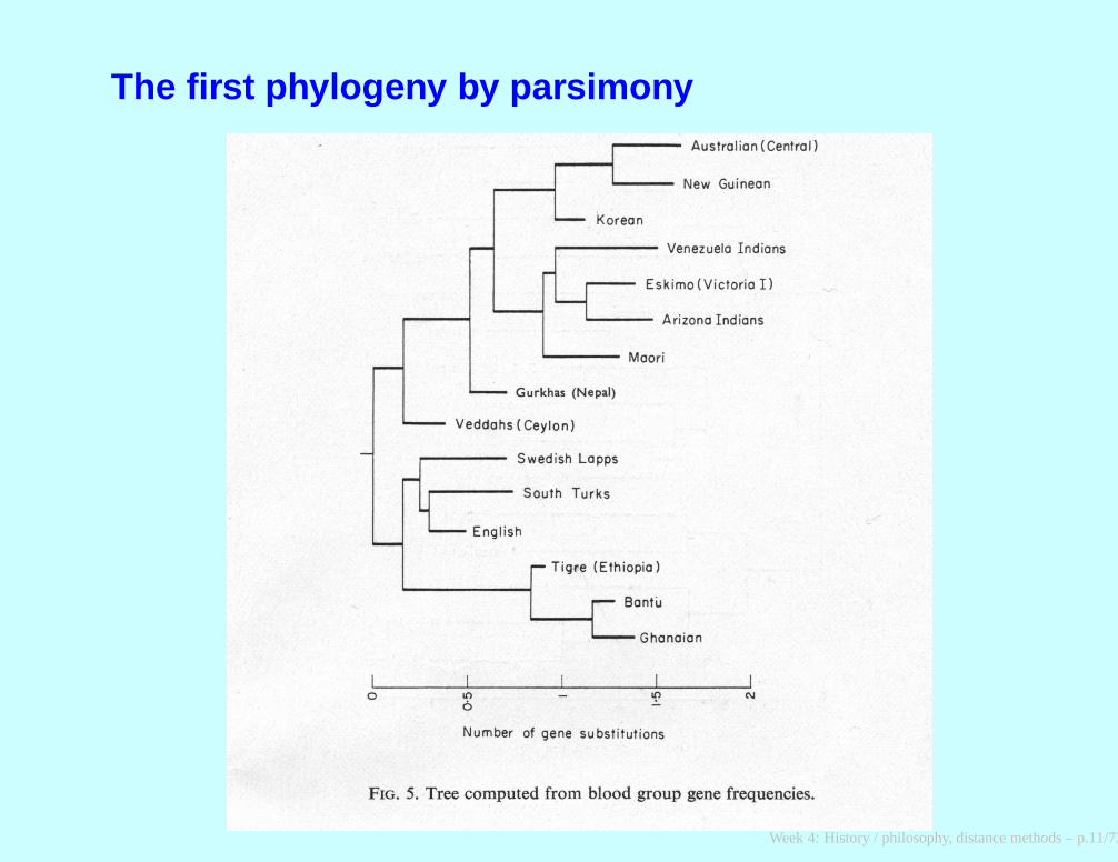
The first phylogeny by parsimony


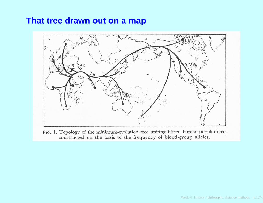
That tree drawn out on a map


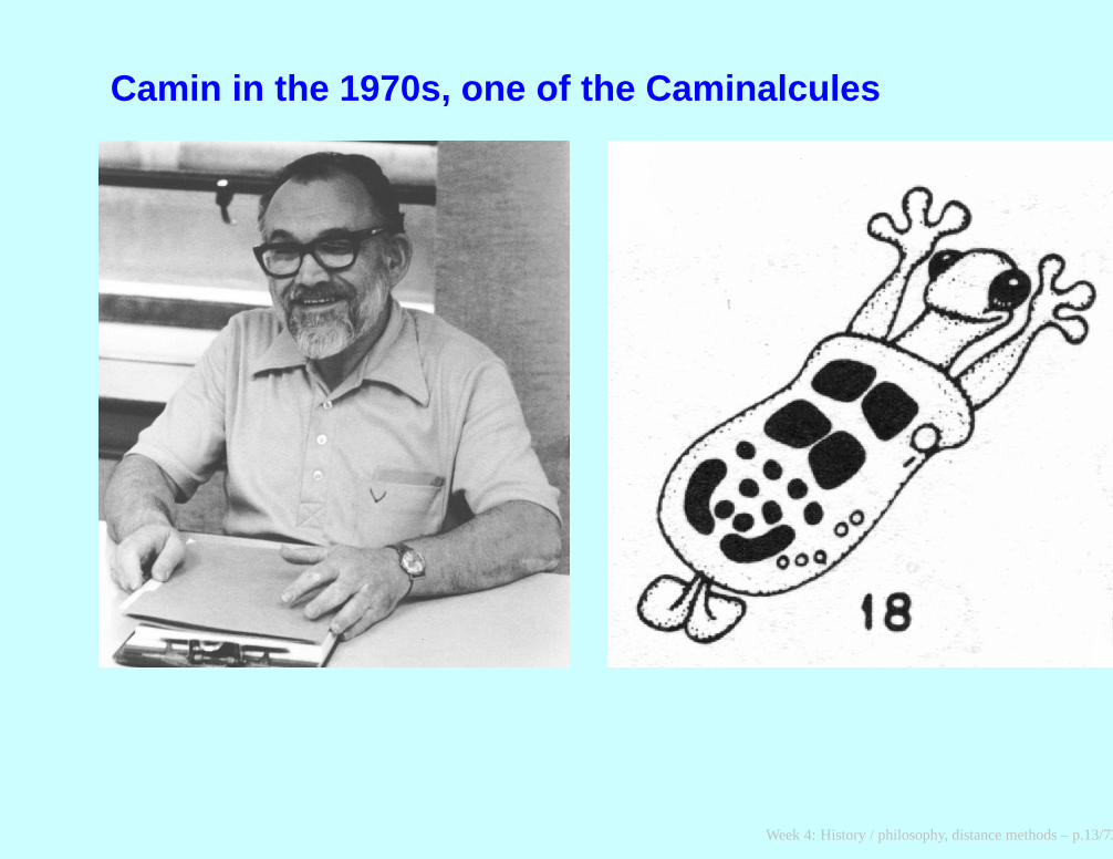
Camin in the 1970s, one of the Caminalcules


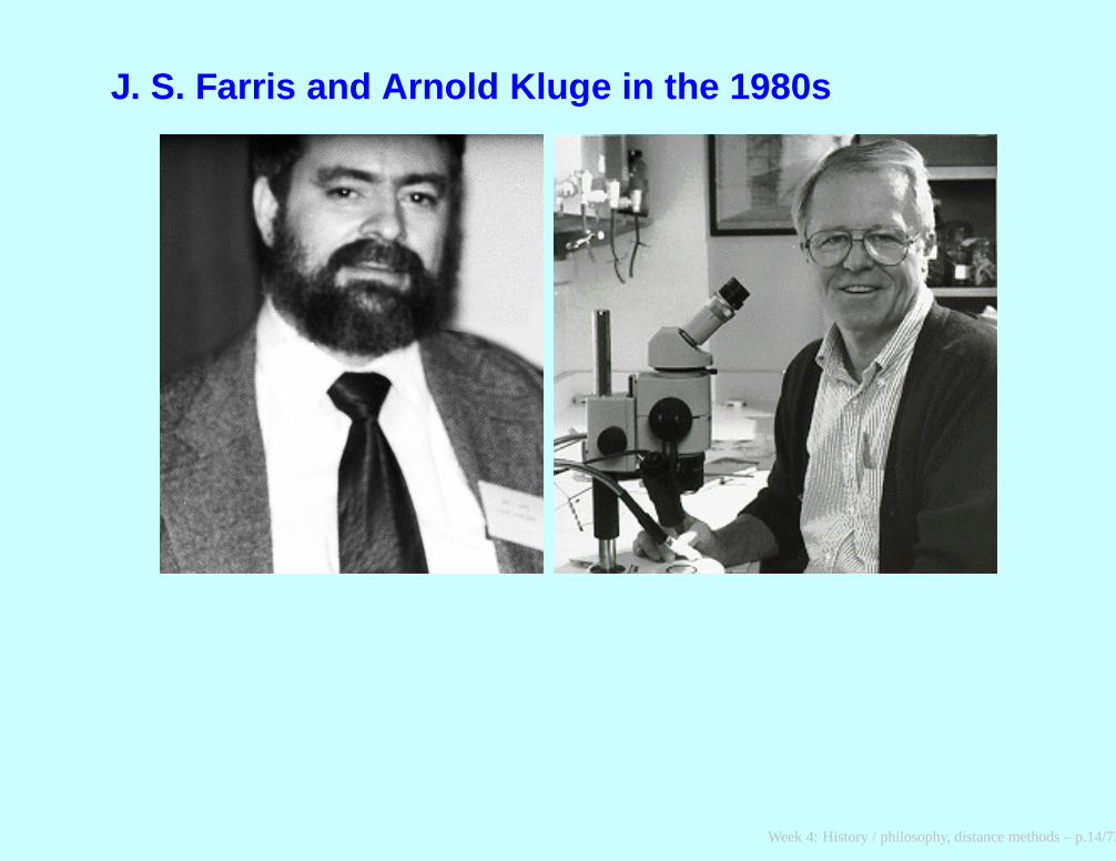
J. S. Farris and Arnold Kluge in the 1980s


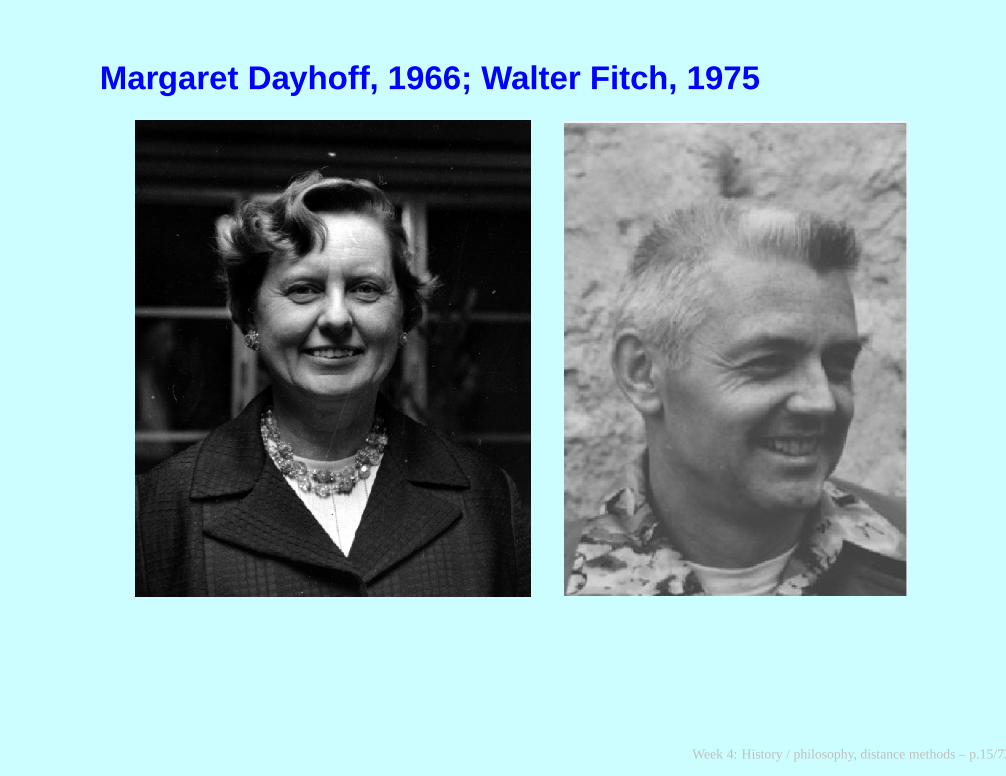
Margaret Dayhoff, 1966; Walter Fitch, 1975


Fitch and Margoliash’s 1967 distance tree


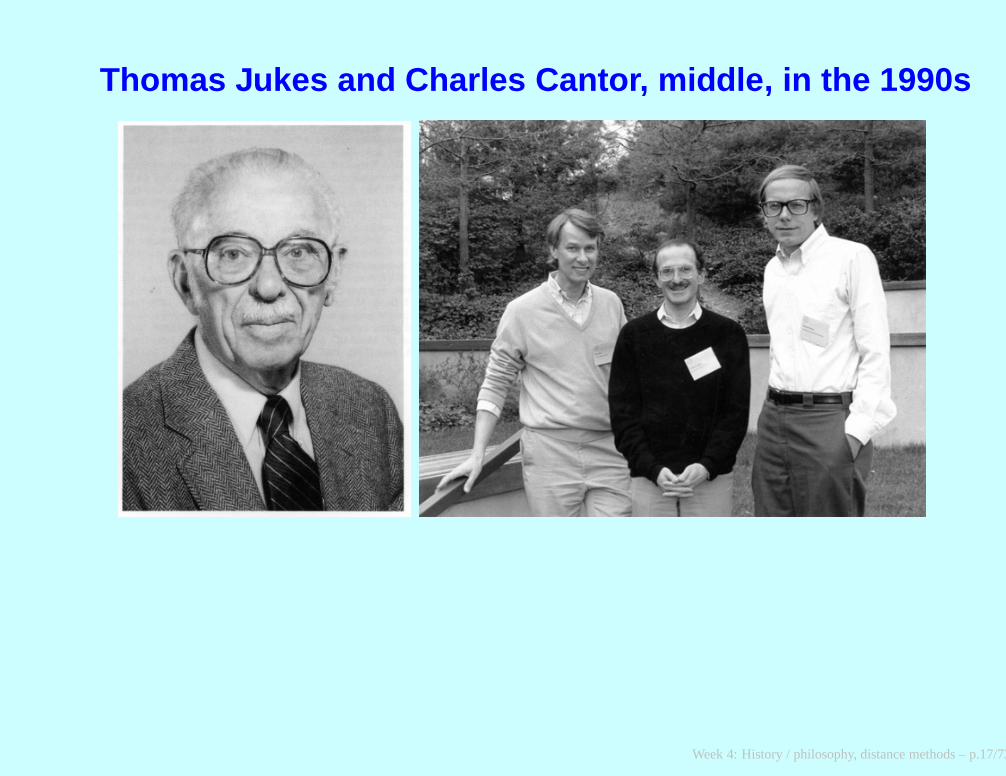
Thomas Jukes and Charles Cantor, middle, in the 1990s


Jerzy Neyman


Willi Hennig (in 1972) and Walter Zimmermann (in 1959)

Willi Hennig (1913-1976) Walter Zimmermann (1890-1980)


Hennig and conflict of characters

W. Hennig (1966) says that in the case of homoplasy,

“it becomes necessary to recheck the interpretation of [the]characters"

He also says (1966, p. 121)

“the more certainly characters interpreted as apomorphous(not characters in general) are present in a number of differentspecies, the better founded is the assumption that thesespecies form a morphological group."

Farris, Kluge, and Eckardt (1970) argue that this should be translated as:

“the more characters certainly interpretable as apomorphous..."


Did Hennig invent parsimony?

Farris (1983, p. 8):

I shall use the term in the sense I have already mentioned:most parsimonious genealogical hypotheses are those thatminimize requirements for ad hoc hypotheses of homoplasy. Ifminimizing ad hoc hypotheses is not the only connotation of“parsimony" in general useage, it is scarcely novel. BothHennig (1966) and Wiley (1975) have advanced ideas closelyrelated to my useage. Hennig defends phylogenetic analysison the grounds of his auxiliary principle, which states thathomology should be presumed in the absence of evidence tothe contrary. This amounts to the precept that homoplasyought not be postulated beyond necessity, that is to sayparsimony.


Hennig’s auxiliary principle

Hennig discusses the case in which “only one character can certainly orwith reasonable probability be interpreted as apomorphous."Hennig (1966, p. 121):

In such cases it is impossible to decide whether the commoncharacter is indeed synapomorphous or is to be interpreted asparallelism, homoiology, or even as convergence. I havetherefore called it an “auxiliary principle" that the presence ofapomorphous characters in different species “is alwaysreason for suspecting kinship [i.e. that the species belong to amonophyletic group], and that their origin by convergenceshould not be assumed a priori" (Hennig 1953). This wasbased on the conviction that “phylogenetic systematics wouldlose all the ground on which it stands" if the presence ofapomorphous characters in different species were consideredfirst of all as convergences (or parallelisms), with proof to thecontrary required in each case.


Farris and Kluge on Hennig and parsimony

Unfortunately, AIV is not sufficiently detailed to allow us toselect a unique criterion for choosing a most preferable tree.We know that trees on which the monophyletic groups sharemany steps are preferable to trees on which this is not so. ButAIV deals only with single monophyletic groups and does nottell us how to evaluate a tree consisting of severalmonophyletic groups. One widely used criterion – parsimony –could be used to select trees. This would be in accord withAIV, since on a most parsimonious tree OTUs [tips] that sharemany states (this is not the same as the OTUs’ being describedby many of the same states) are generally placed together. Wemight argue that the parsimony criterion selects a tree most inaccord with AIV by “averaging" in some sense the preferabilityof all the monophyletic groups of the tree. Other criteria,however, may also agree with AIV.

Farris, Eckardt and Kluge, 1970


Philosophical frameworks: hypothetico-deductive

Gaffney (1979, pp. 98-99)

In any case, in a hypothetico-deductive system, parsimony isnot merely a methodological convention, it is a direct corollaryof the falsification criterion for hypotheses (Popper, 1968a, pp.144-145). When we accept the hypothetico-deductive systemas a basis for phylogeny reconstruction, we try to test a seriesof phylogenetic hypotheses in the manner indicated above. Ifall three of the three possible three-taxon statements arefalsified at least once, the least-rejected hypothesis remainsas the preferred one, not because of an arbitrarymethodological rule, but because it best meets our criterion oftestability. In order to accept an hypothesis that has beensuccessfully falsified one or more times, we must adopt an adhoc hypothesis for each falsification .... Therefore, in a systemthat seeks to maximize vulnerability to criticism, the addition ofad hoc hypotheses must be kept to a minimum to meet thiscriterion.


more from Gaffney

Gaffney (1979)

“the use of derived character distributions as articulated byHennig (1966) appears to fit the hypothetico-deductive modelbest."

Gaffney (1979, p. 98)

“it seems to me that parsimony, or Ockham’s razor, isequivalent to ‘logic’ or ‘reason’ because any method that doesnot follow the above principle would be incompatible with anykind of predictive or causal system."


Hypothetico-deductivists on falsification

Eldredge and Cracraft (1980, p. 69) are careful to point out that

“Falsified" implies that the hypotheses are proven false, butthis is not the meaning we (or other phylogenetic systematists)wish to convey. It may be that the preferred hypothesis willitself be “rejected" by some synapomorphies.

Wiley (1981, p. 111):

In other words, we have no external criterion to say that aparticular conflicting character is actually an invalid test.Therefore, saying that it is an invalid test simply because it isunparsimonious is a statement that is, itself, an ad hocstatement. With no external criterion, we are forced to useparsimony to minimize the total number of ad hoc hypotheses(Popper, 1968a: 145). The result is that the mostparsimonious of the various alternates is the most highlycorroborated and therefore preferred over the lessparsimonious alternates.


Farris on hypothetico-deductivism

Farris (1983, p. 8):

Wiley [(1975)] discusses parsimony in a Popperian context,characterizing most parsimonious genealogies as those thatare least falsified on available evidence. In his treatment,contradictory character distributions provide putative falsifiersof genealogies. As I shall discuss below, any such falsifierengenders a requirement for an ad hoc hypothesis ofhomoplasy to defend the genealogy. Wiley’s concept is thenequivalent to mine.


Philosophical frameworks: Logical-parsimony

Beatty and Fink (1979):

We can account for the necessity of parsimony (or some suchconsideration) because evidence considerations alone are notsufficient. But we have no philosophical or logical argumentwith which to justify the use of parsimony considerations – anot surprising result, since this issue has remained aphilosophical dilemma for hundreds of years.


Kluge and Wolf on logical parsimony

Kluge and Wolf (1993, p. 196):

Finally, we might imagine that some of the popularity of theaforementioned methodological strategies and resamplingtechniques, and assumption of independence in the context oftaxonomic congruence and the cardinal rule of Brooks andMcLennan (1991), derives from the belief that phylogeneticinference is hypothetico-deductive (e.g. Nelson and Platnick,1984: 143-144), or at least that it should be. Even the uses towhich some might put cladograms, such as “testing"adaptation (Coddington, 1988), are presented ashypothetico-deductive. But this ignores an alternative, thatcladistics, and its uses, may be an abductive enterprise(Sober, 1988). We suggest that the limits of phylogeneticsystematics will be clarified considerably when cladistsunderstand how their knowledge claims are made (Rieppel,1988; Panchen, 1992).


Elliot Sober on falsificationSober (1988, p. 126):

Popper’s philosophy of science is very little help here,because he has little to say about weak falsification. Popper,after all is a hypothetico-deductivist. For him, observationalclaims are deductive consequences of the hypothesis undertest .... Deductivism excludes the possibility of probabilistictesting. A theory that assigns probabilities to various possibleobservational outcomes cannot be strongly falsified by theoccurrence of any of them. This, I suggest, is the situation weconfront in testing phylogenetic hypotheses. (AB)C is logicallyconsistent with all possible character distributions (polarized ornot), and the same is true of A(BC). [Emphasis in the original]


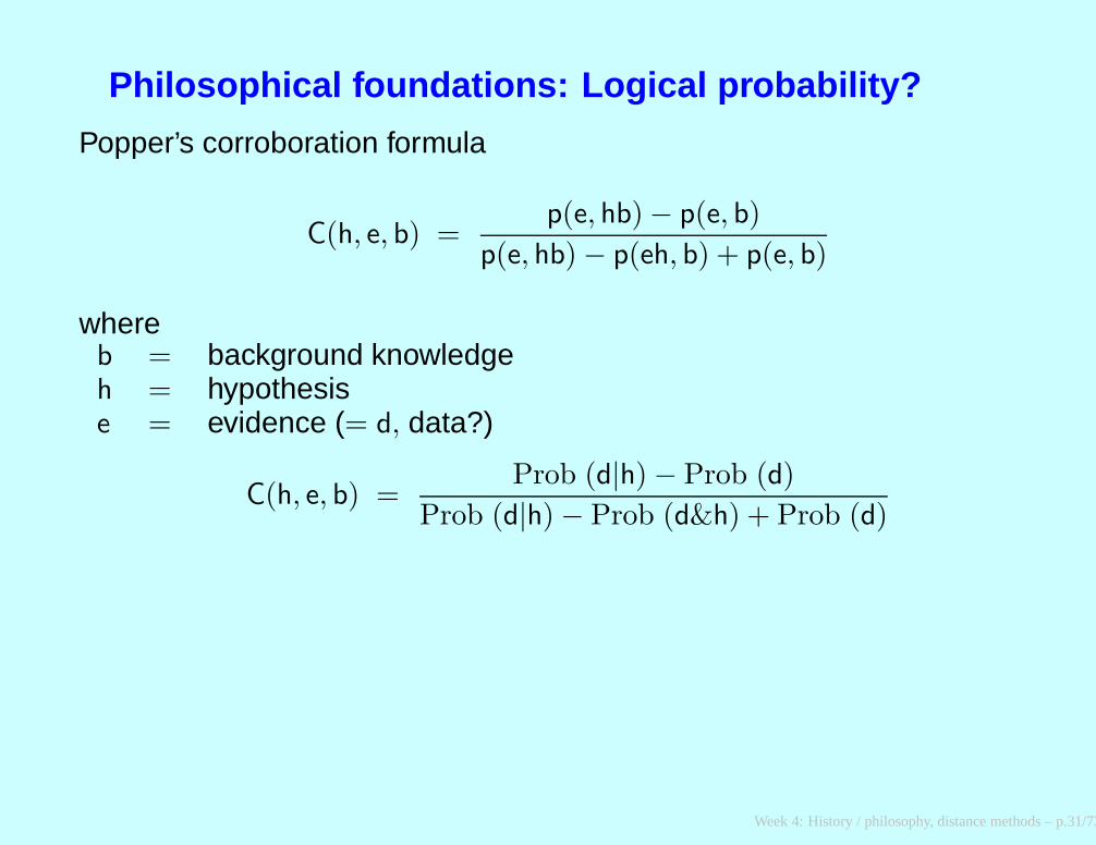
Philosophical foundations: Logical probability?

Popper’s corroboration formula

C(h, e, b) =p(e, hb) − p(e, b)

p(e, hb) − p(eh, b) + p(e, b)

whereb = background knowledgeh = hypothesise = evidence (= d, data?)

C(h, e, b) =Prob (d|h) − Prob (d)

Prob (d|h) − Prob (d&h) + Prob (d)


Criticisms of statistical inferenceFarris (1983, p.17):

The statistical approach to phylogenetic inference was wrongfrom the start, for it rests on the idea that to study phylogenyat all, one must first know in great detail how evolution hasproceeded.

Kluge (1997a)

“As an aside, the fact that the study of phylogeny is concernedwith the discovery of historical singularities means thatcalculus probability and standard (Neyman-Pearson) statisticscannot apply to that historical science ...."


Positions on classification nowadays

Phylogenetic systematics. Willi Hennig advocated purelymonophyletic classification. Now the (strongly) dominant approach.

Evolutionary systematics. Has almost faded away. Its adherentswere reluctant to make it algorithmic.

Phenetics. Although Sokal and Sneath strongly influenced the fieldof numerical clustering, their approach to biological classificationhas few adherents.IDMVM One person (me) takes the view that It Doesn’t Matter VeryMuch, as we use the phylogeny, and, given that, we never use theclassification system. This is widely regarded as a marginalcrackpot view [“A bizarre thumb in the eye to systematists” –Michael Sanderson].


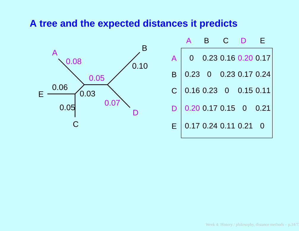
A tree and the expected distances it predicts

A B C D E

A

B

C

D

E

0

0

0

0

0

0.23 0.16 0.20 0.17

0.23 0.17 0.24

0.15 0.11

0.21

0.23

0.16

0.20

0.17

0.23

0.17

0.24

0.15

0.11 0.21

0.10

0.07

0.05

0.08

0.030.06

0.05

A B

CD

E


A tree and a set of two-species trees

0.10

0.07

0.05

0.08

0.030.06

0.05

A B

CD

E

A

CD

E

B

The two-species trees correspond to the pairwise distances observedbetween the pairs of species.


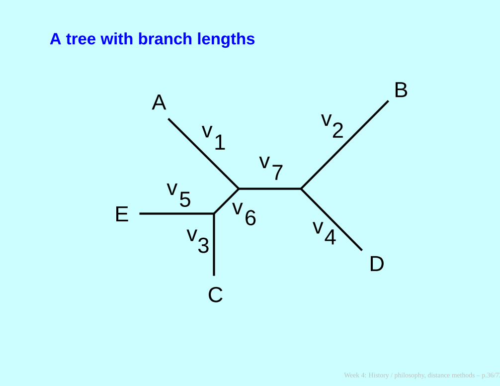
A tree with branch lengths

A B

CD

E

v1v2

v3v4

v5 v6

v7


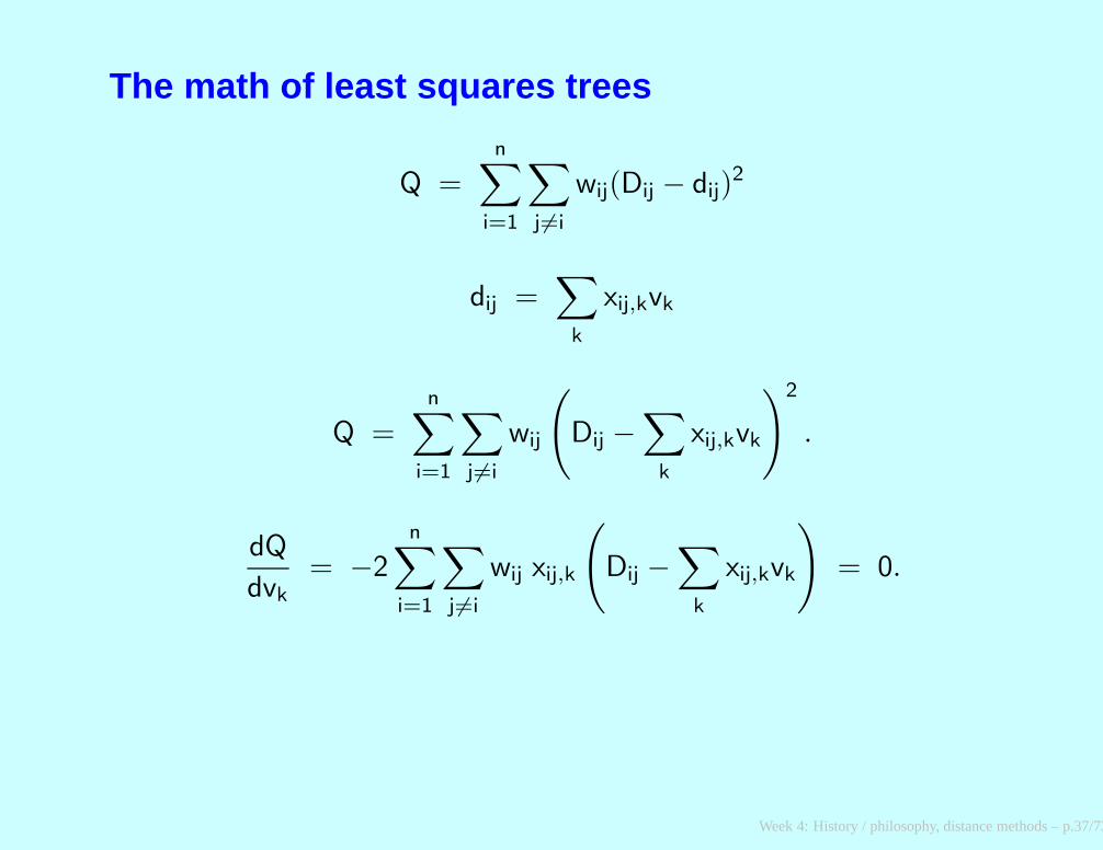
The math of least squares trees

Q =n∑

i=1

∑

j6=i

wij(Dij − dij)2

dij =∑

k

xij,kvk

Q =n∑

i=1

∑

j6=i

wij

(Dij −

∑

k

xij,kvk

)2

.

dQ

dvk

= −2

n∑

i=1

∑

j6=i

wij xij,k

(

Dij −∑

k

xij,kvk

)

= 0.


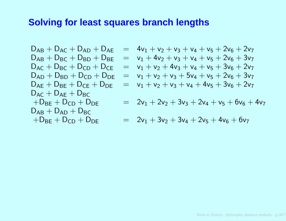
Solving for least squares branch lengths

DAB + DAC + DAD + DAE = 4v1 + v2 + v3 + v4 + v5 + 2v6 + 2v7

DAB + DBC + DBD + DBE = v1 + 4v2 + v3 + v4 + v5 + 2v6 + 3v7

DAC + DBC + DCD + DCE = v1 + v2 + 4v3 + v4 + v5 + 3v6 + 2v7

DAD + DBD + DCD + DDE = v1 + v2 + v3 + 5v4 + v5 + 2v6 + 3v7

DAE + DBE + DCE + DDE = v1 + v2 + v3 + v4 + 4v5 + 3v6 + 2v7

DAC + DAE + DBC

+DBE + DCD + DDE = 2v1 + 2v2 + 3v3 + 2v4 + v5 + 6v6 + 4v7

DAB + DAD + DBC

+DBE + DCD + DDE = 2v1 + 3v2 + 3v4 + 2v5 + 4v6 + 6v7


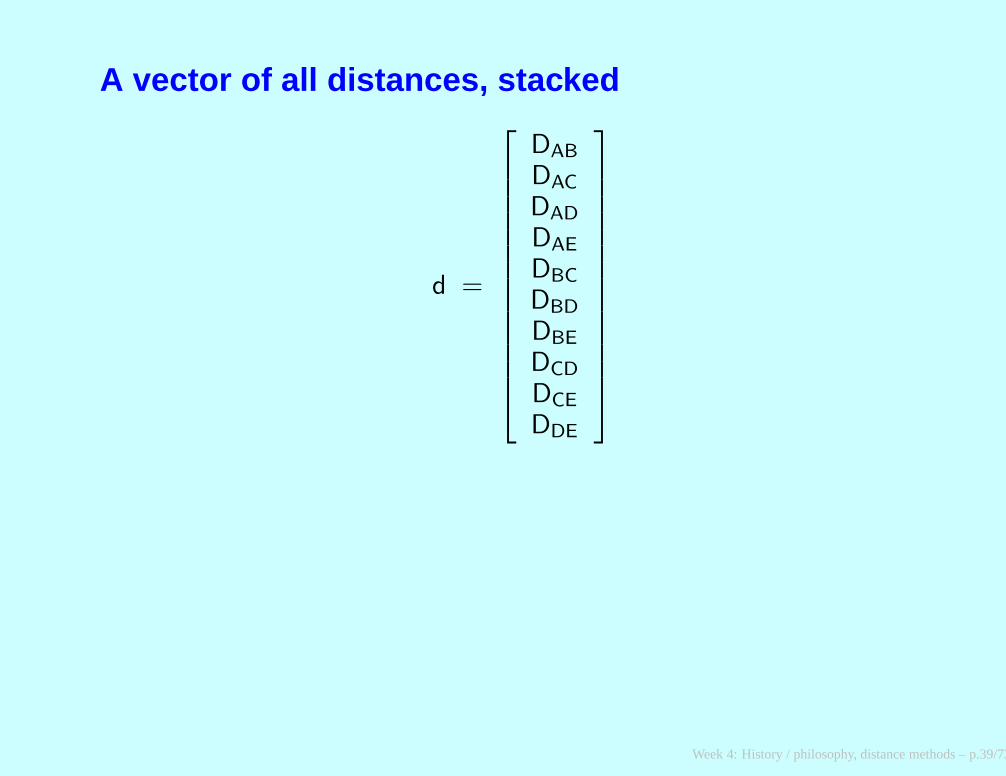
A vector of all distances, stacked

d =

DAB

DAC

DAD

DAE

DBC

DBD

DBE

DCD

DCE

DDE


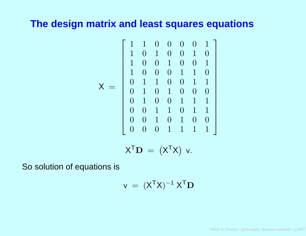
The design matrix and least squares equations

X =

1 1 0 0 0 0 11 0 1 0 0 1 01 0 0 1 0 0 11 0 0 0 1 1 00 1 1 0 0 1 10 1 0 1 0 0 00 1 0 0 1 1 10 0 1 1 0 1 10 0 1 0 1 0 00 0 0 1 1 1 1

XTD =(XTX

)v.

So solution of equations is

v = (XTX)−1 XTD


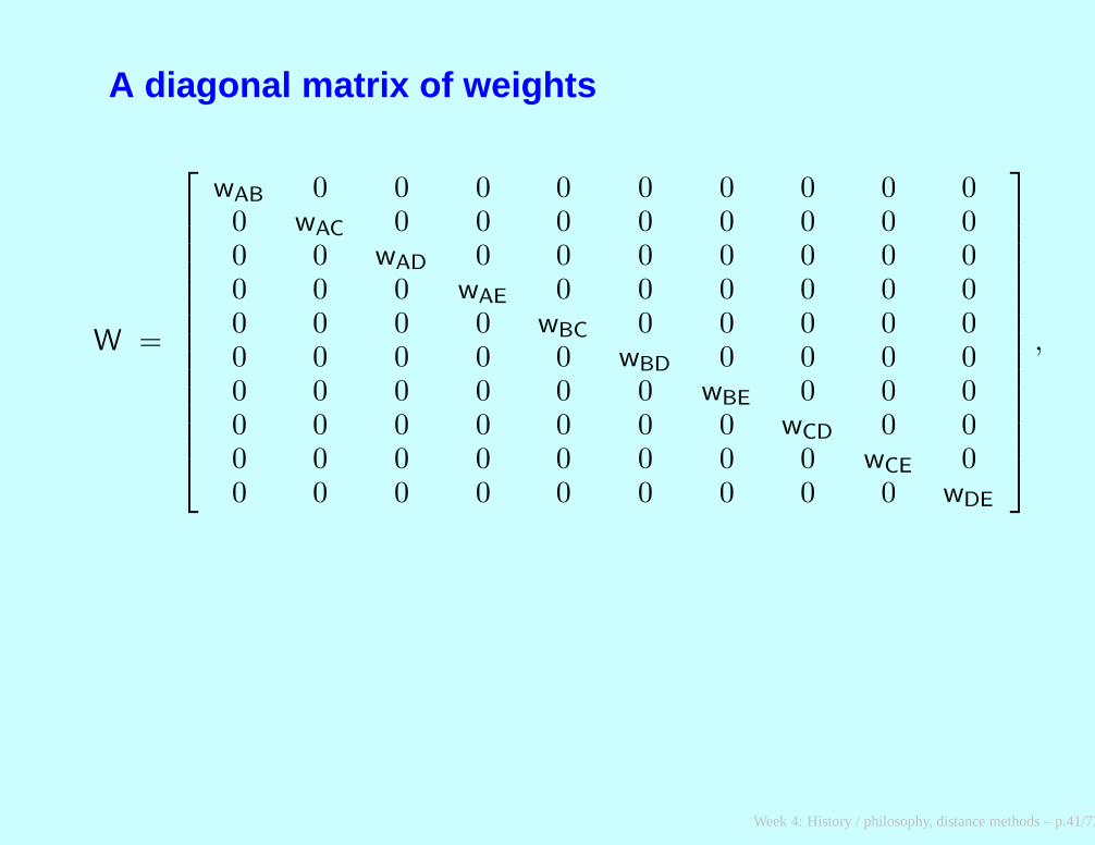
A diagonal matrix of weights

W =

wAB 0 0 0 0 0 0 0 0 00 wAC 0 0 0 0 0 0 0 00 0 wAD 0 0 0 0 0 0 00 0 0 wAE 0 0 0 0 0 00 0 0 0 wBC 0 0 0 0 00 0 0 0 0 wBD 0 0 0 00 0 0 0 0 0 wBE 0 0 00 0 0 0 0 0 0 wCD 0 00 0 0 0 0 0 0 0 wCE 00 0 0 0 0 0 0 0 0 wDE

,


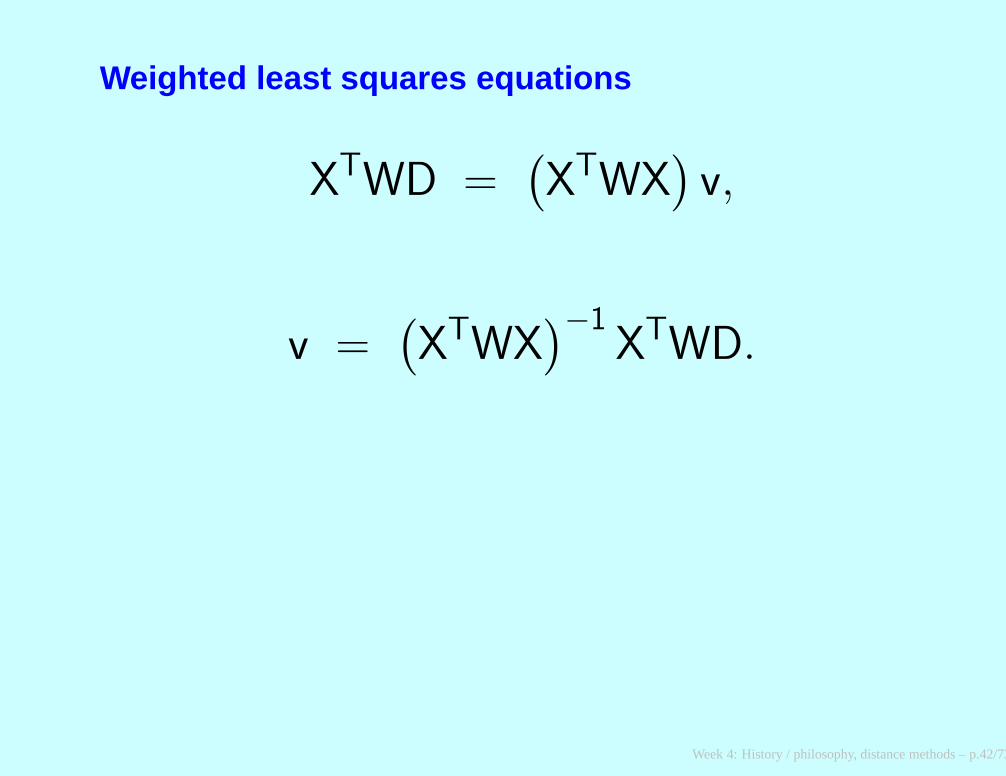
Weighted least squares equations

XTWD =

(X

TWX)v,

v =

(X

TWX)−1

XTWD.


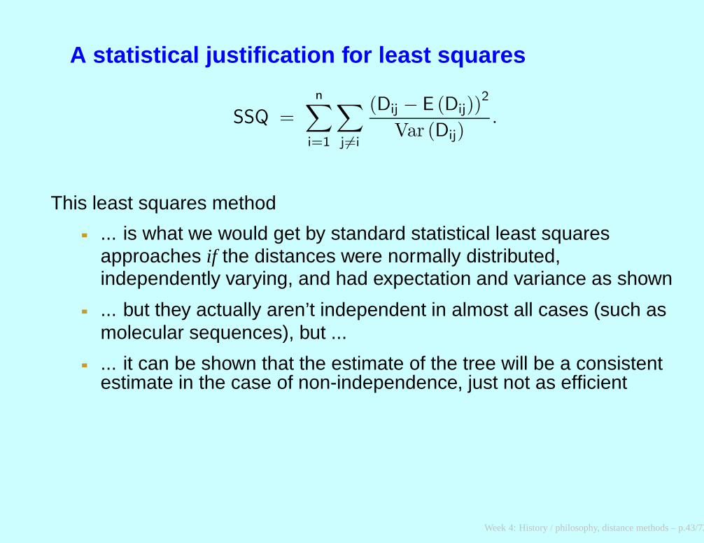
A statistical justification for least squares

SSQ =n∑

i=1

∑

j6=i

(Dij − E (Dij))2

Var (Dij).

This least squares method

... is what we would get by standard statistical least squaresapproaches if the distances were normally distributed,independently varying, and had expectation and variance as shown

... but they actually aren’t independent in almost all cases (such asmolecular sequences), but ...

... it can be shown that the estimate of the tree will be a consistentestimate in the case of non-independence, just not as efficient


The Jukes-Cantor model

A G

C T

u/3

u/3

u/3u/3 u/3

u/3


The Jukes-Cantor modelProbability of no event:

e−43ut

Probability of some event:

1 − e−43ut

Probability of changing to C given start at A, have rate u, time t:

Prob (C|A, u, t) =1

4

(1 − e−

43ut)

fraction of sites different:

DS =3

4

(1 − e−

43ut)

.

distance as function of fraction of sites different

D = ut = −3

4ln

(1 −

4

3DS

)


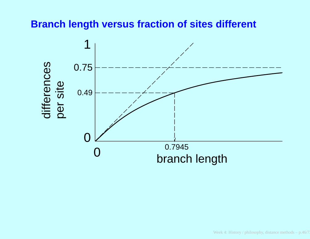
Branch length versus fraction of sites different

0

1

0

0.75

0.49

0.7945

per

site

diffe

renc

es

branch length


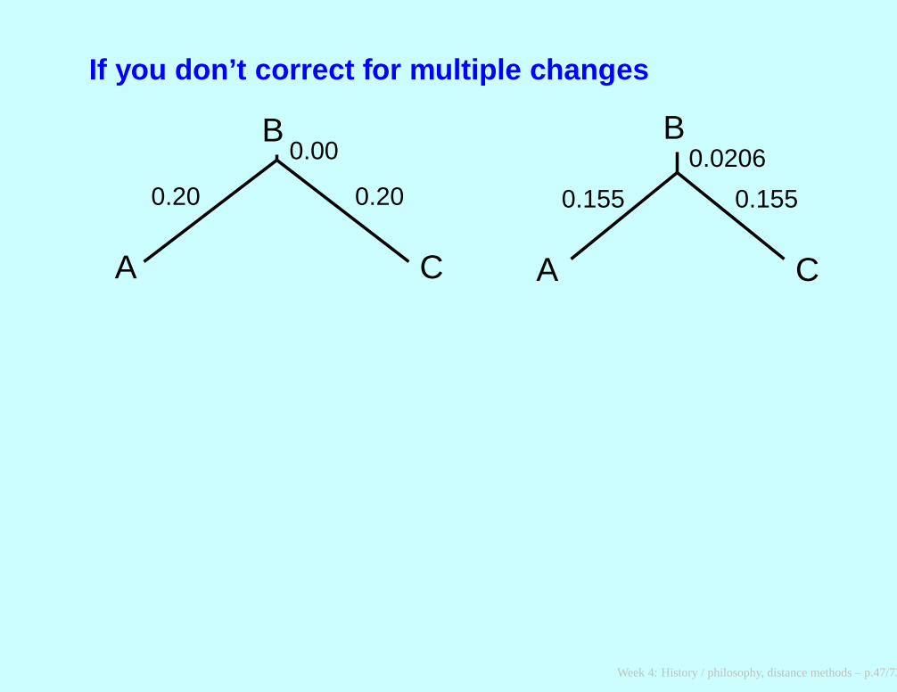
If you don’t correct for multiple changes

A

B

C

0.155 0.155

0.0206

A

B

C

0.20 0.20

0.00


The Minimum Evolution method

Kidd and Sgaramella-Zonta (1971) and (independently) Rzhetsky and Nei(1992ff.) came up with this method:

Search through tree space as usual

For each tree estimate branch lenghts by least squares, not allowingnegative branch lengths

Then actually evaluate the tree not by the sum of squares, but by thetotal sum of branch lengths.

This does fairly well, in spite of the mixture of two optimization criteria.

Note that it is not directly related to parsimony, in spite of its name.


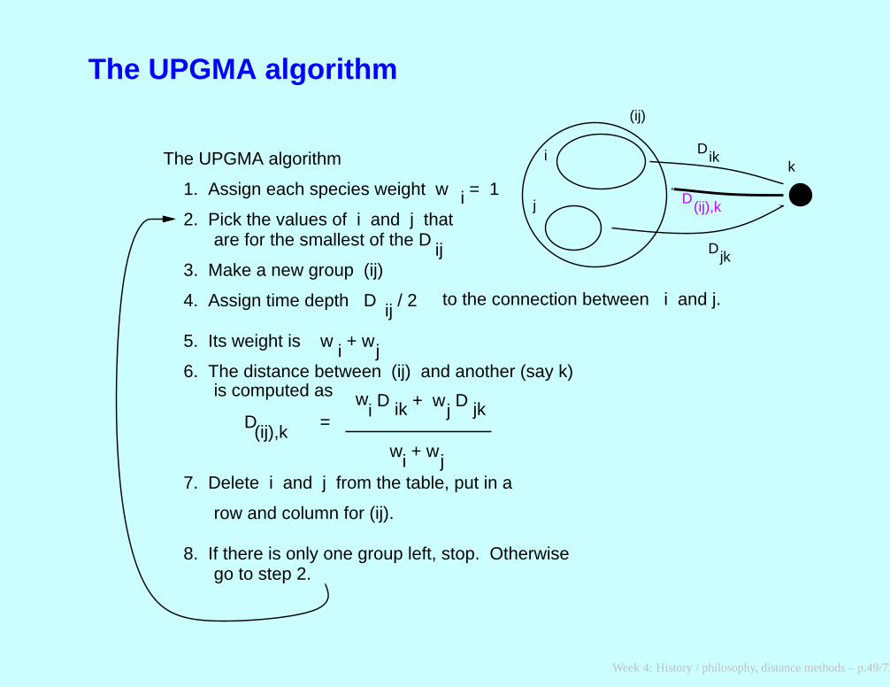
The UPGMA algorithm

i

j

kDik

Djk

D

(ij)

(ij),k

The UPGMA algorithm

= 1

2. Pick the values of i and j thatare for the smallest of the D ij

3. Make a new group (ij)

+ wj

D(ij),k =

wi + wj

row and column for (ij).

5. Its weight is w

6. The distance between (ij) and another (say k)

7. Delete i and j from the table, put in a

8. If there is only one group left, stop. Otherwisego to step 2.

is computed asi + wj jkw

1. Assign each species weight w i

ik

ij / 2

i

D D

4. Assign time depth D to the connection between i and j.


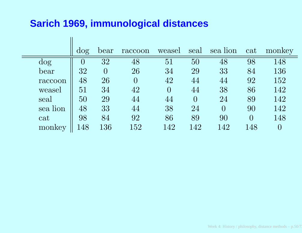
Sarich 1969, immunological distances

dog bear raccoon weasel seal sea lion cat monkey

dog 0 32 48 51 50 48 98 148bear 32 0 26 34 29 33 84 136raccoon 48 26 0 42 44 44 92 152weasel 51 34 42 0 44 38 86 142seal 50 29 44 44 0 24 89 142sea lion 48 33 44 38 24 0 90 142cat 98 84 92 86 89 90 0 148monkey 148 136 152 142 142 142 148 0


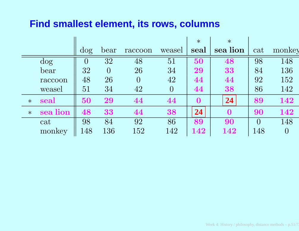
Find smallest element, its rows, columns

∗ ∗dog bear raccoon weasel seal sea lion cat monkey

dog 0 32 48 51 50 48 98 148bear 32 0 26 34 29 33 84 136raccoon 48 26 0 42 44 44 92 152weasel 51 34 42 0 44 38 86 142

∗ seal 50 29 44 44 0 24 89 142

∗ sea lion 48 33 44 38 24 0 90 142

cat 98 84 92 86 89 90 0 148monkey 148 136 152 142 142 142 148 0


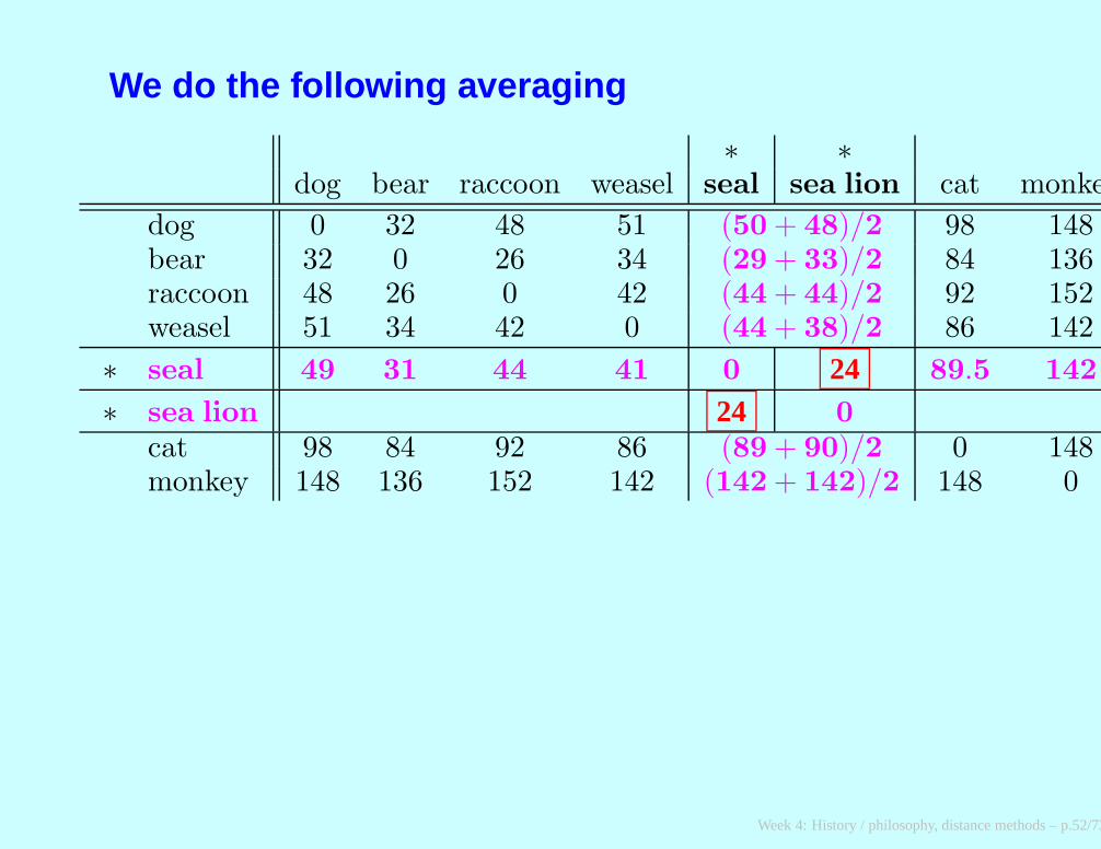
We do the following averaging

∗ ∗dog bear raccoon weasel seal sea lion cat monkey

dog 0 32 48 51 (50 + 48)/2 98 148bear 32 0 26 34 (29 + 33)/2 84 136raccoon 48 26 0 42 (44 + 44)/2 92 152weasel 51 34 42 0 (44 + 38)/2 86 142

∗ seal 49 31 44 41 0 24 89.5 142

∗ sea lion 24 0

cat 98 84 92 86 (89 + 90)/2 0 148monkey 148 136 152 142 (142 + 142)/2 148 0


Clustering seal and sea lion

dog

bear

racc

oon

seal

sea

lion

wea

sel

cat

mon

key

12 12


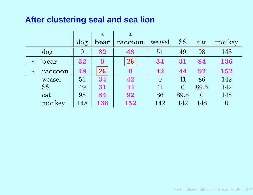
After clustering seal and sea lion

∗ ∗dog bear raccoon weasel SS cat monkey

dog 0 32 48 51 49 98 148

∗ bear 32 0 26 34 31 84 136

∗ raccoon 48 26 0 42 44 92 152

weasel 51 34 42 0 41 86 142SS 49 31 44 41 0 89.5 142cat 98 84 92 86 89.5 0 148monkey 148 136 152 142 142 148 0


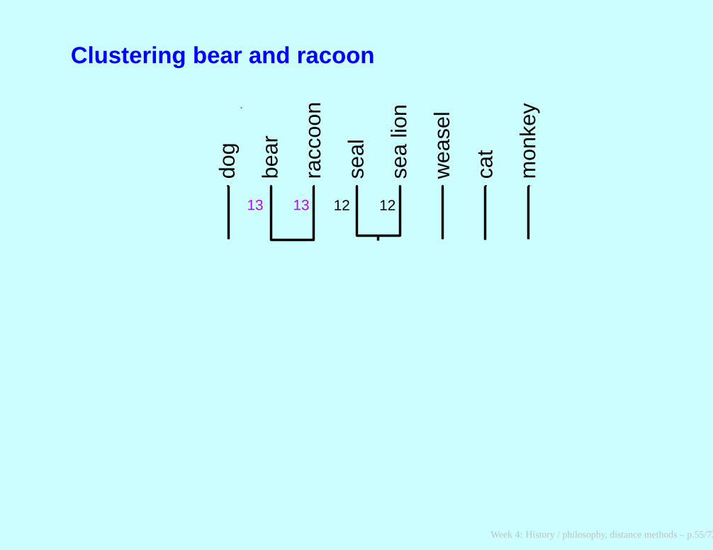
Clustering bear and racoon

dog

bear

racc

oon

seal

sea

lion

wea

sel

cat

mon

key

13 13 12 12


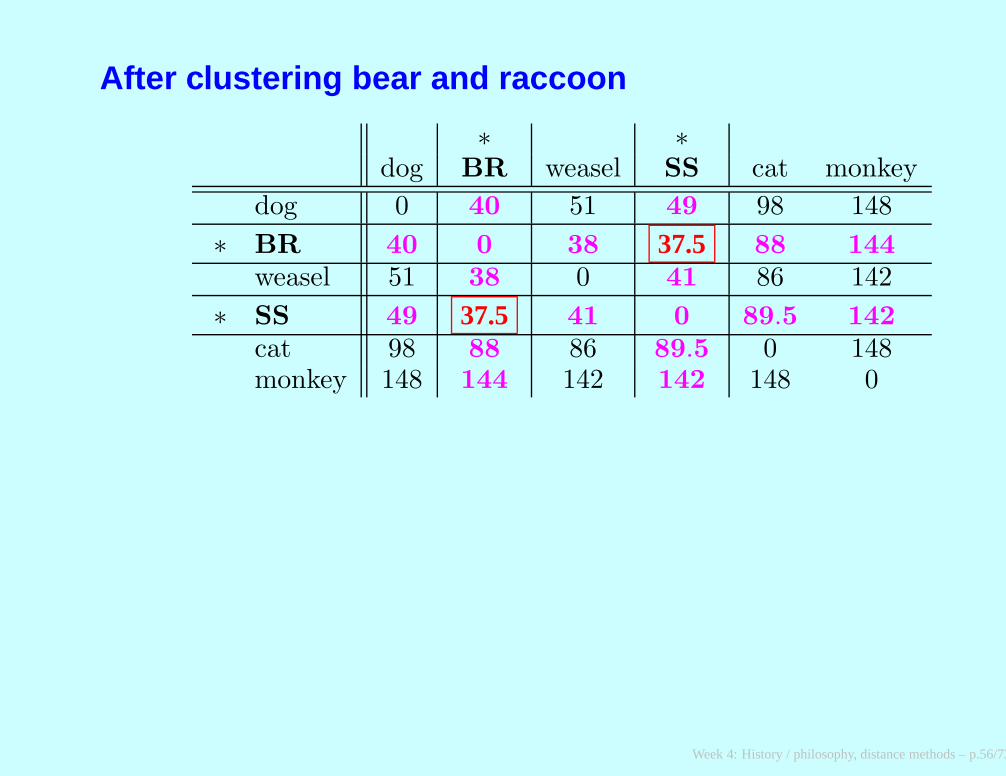
After clustering bear and raccoon

∗ ∗dog BR weasel SS cat monkey

dog 0 40 51 49 98 148

∗ BR 40 0 38 37.5 88 144

weasel 51 38 0 41 86 142

∗ SS 49 37.5 41 0 89.5 142

cat 98 88 86 89.5 0 148monkey 148 144 142 142 148 0


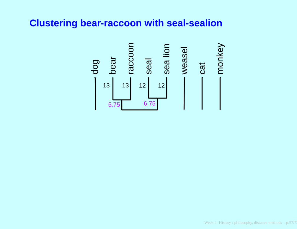
Clustering bear-raccoon with seal-sealion

dog

bear

racc

oon

seal

sea

lion

wea

sel

cat

mon

key

5.75 6.75

13 13 12 12


After clustering those two clusters

∗ ∗dog BRSS weasel cat monkey

dog 0 44.5 51 98 148

∗ BRSS 44.5 0 39.5 88.75 143

∗ weasel 51 39.5 0 86 142

cat 98 88.75 86 0 148monkey 148 143 142 148 0


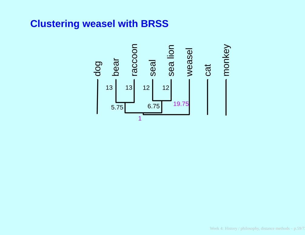
Clustering weasel with BRSS

dog

bear

racc

oon

seal

sea

lion

wea

sel

cat

mon

key

5.75 6.75 19.75

13 13 12 12

1


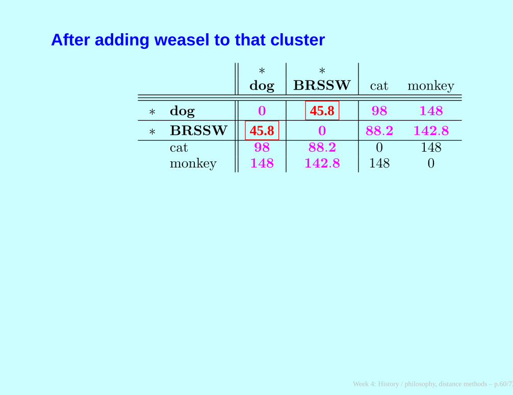
After adding weasel to that cluster

∗ ∗dog BRSSW cat monkey

∗ dog 0 45.8 98 148

∗ BRSSW 45.8 0 88.2 142.8cat 98 88.2 0 148monkey 148 142.8 148 0


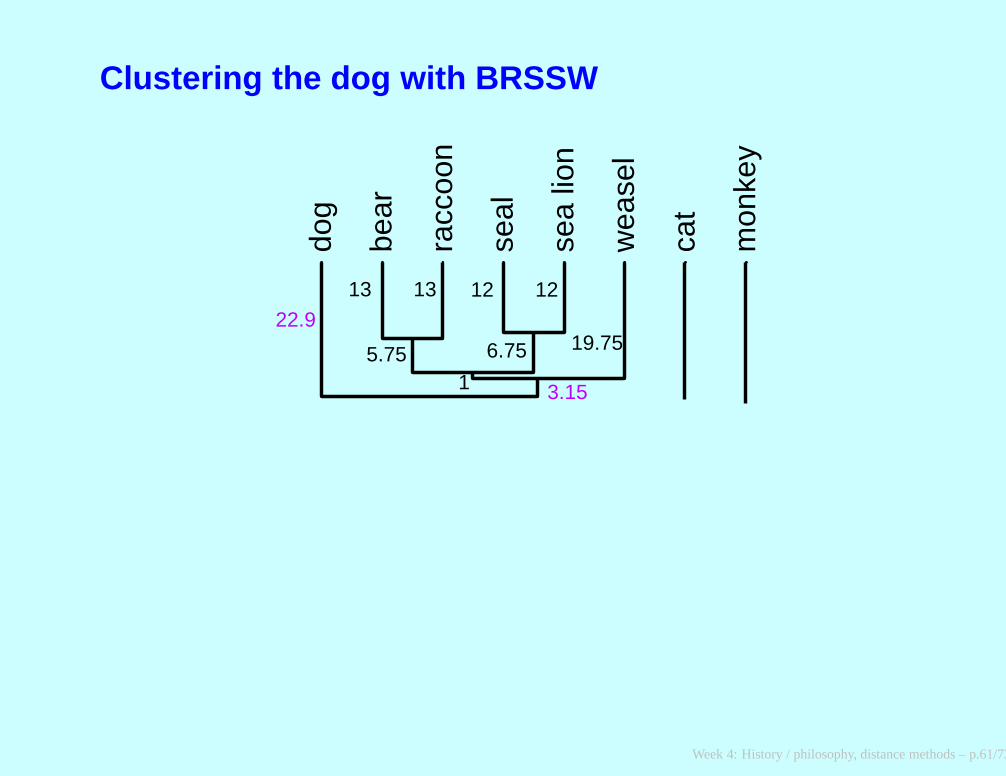
Clustering the dog with BRSSW

dog

bear

racc

oon

seal

sea

lion

wea

sel

cat

mon

key

5.75 6.75 19.75

3.15

22.9

1

13 13 12 12


After adding dog to it

∗ ∗DBRWSS cat monkey

∗ DBRWSS 0 89.833 143.66

∗ cat 89.833 0 148

monkey 143.66 148 0


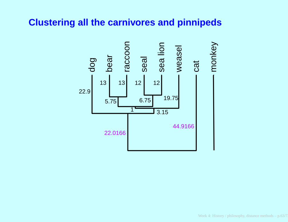
Clustering all the carnivores and pinnipeds

dog

bear

racc

oon

seal

sea

lion

wea

sel

cat

mon

key

5.75 6.75 19.75

3.15

22.9

22.016644.9166

1

13 13 12 12


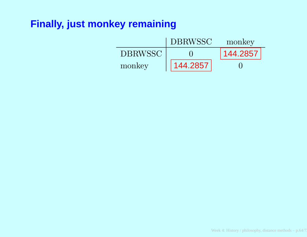
Finally, just monkey remaining

DBRWSSC monkey

DBRWSSC 0 144.2857monkey 144.2857 0


The UPGMA tree

dog

bear

racc

oon

seal

sea

lion

wea

sel

cat

mon

key

5.75 6.75 19.75

3.15

22.9

22.016644.9166

27.22619 72.1428

1

13 13 12 12


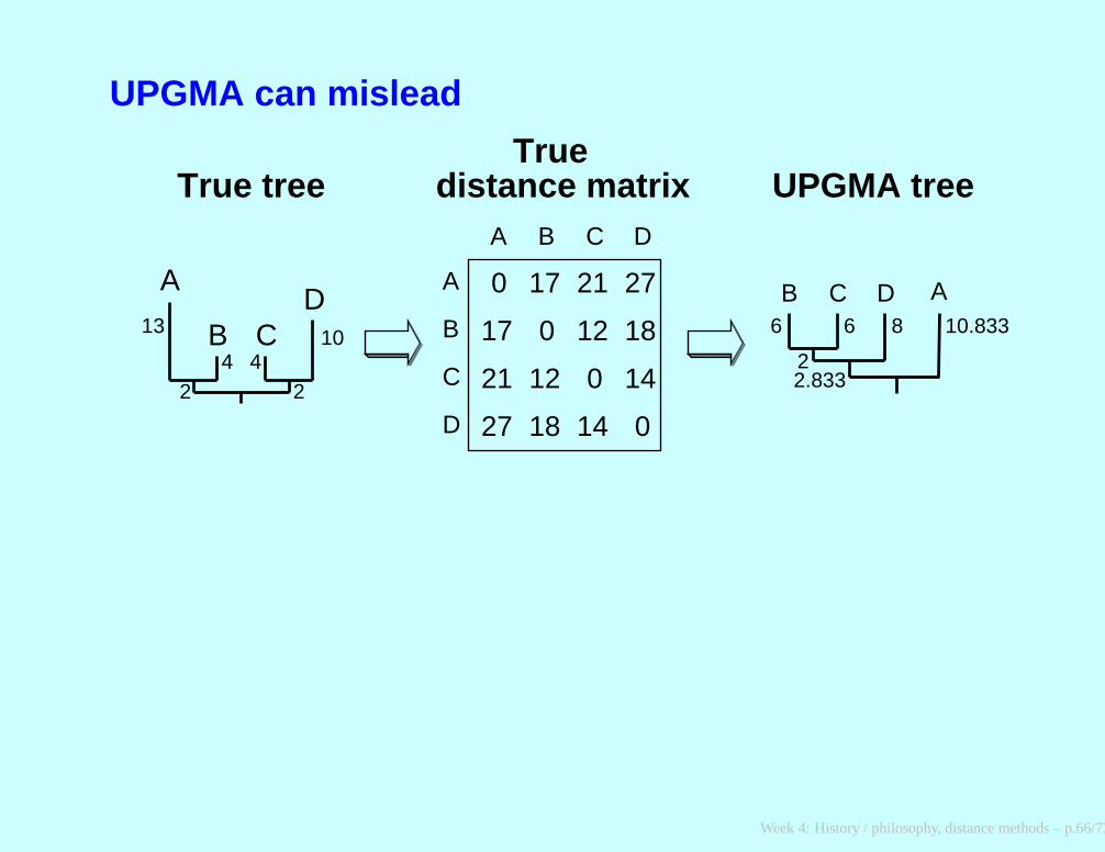
UPGMA can mislead

A

B CD

13

4 410

2 2

A

B

C

D

A B C D

0 17 21 27

17

21

27

0 12 18

12

18

0 14

14 0

B C D A

True tree UPGMA tree

6 6 8 10.833

2.8332

Truedistance matrix


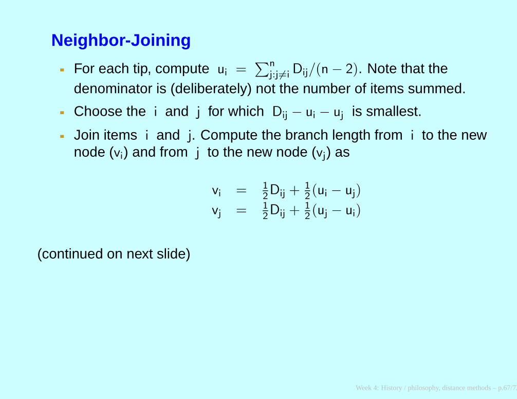
Neighbor-Joining

For each tip, compute ui =∑n

j:j6=i Dij/(n − 2). Note that thedenominator is (deliberately) not the number of items summed.

Choose the i and j for which Dij − ui − uj is smallest.

Join items i and j. Compute the branch length from i to the newnode (vi) and from j to the new node (vj) as

vi = 12Dij +

12(ui − uj)

vj = 12Dij +

12(uj − ui)

(continued on next slide)


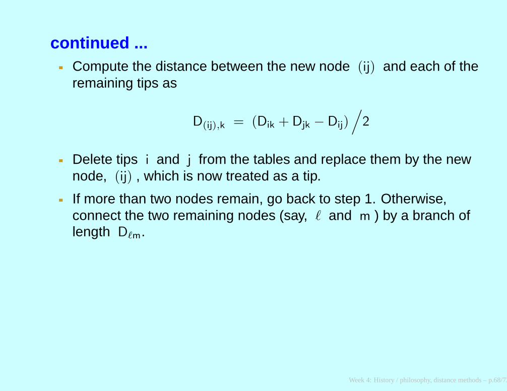
continued ...Compute the distance between the new node (ij) and each of theremaining tips as

D(ij),k = (Dik + Djk − Dij)/

2

Delete tips i and j from the tables and replace them by the newnode, (ij) , which is now treated as a tip.

If more than two nodes remain, go back to step 1. Otherwise,connect the two remaining nodes (say, ℓ and m ) by a branch oflength Dℓm.


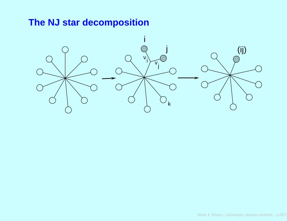
The NJ star decomposition

ij (ij)

vi vj

k


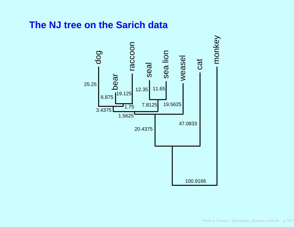
The NJ tree on the Sarich data

dog

bear

racc

oon

seal

sea

lion

wea

sel

cat mon

key

19.5625

20.437547.0833

100.9166

1.56253.4375

25.25

1.75

6.87519.125

7.8125

12.35 11.65


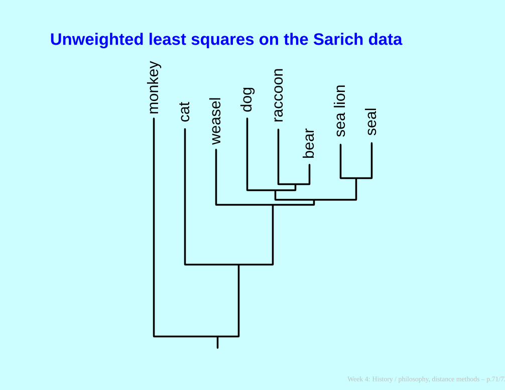
Unweighted least squares on the Sarich data

mon

key

cat

wea

sel

dog

racc

oon

bear se

a lio

n

seal


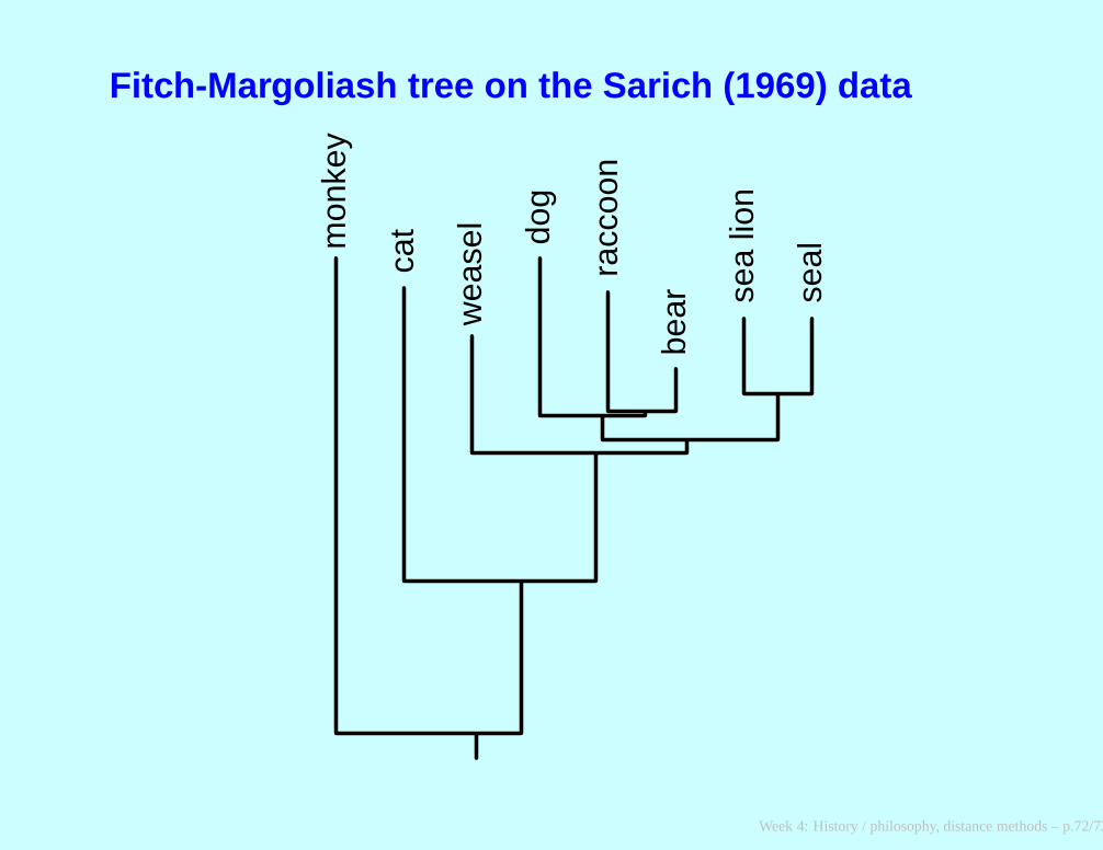
Fitch-Margoliash tree on the Sarich (1969) data

mon

key

cat

wea

sel do

g

racc

oon

bear se

a lio

n

seal


Minimum evolution tree on the Sarich (1969) data

mon

key

cat

wea

sel

racc

oon

dog

bear se

a lio

n

seal


Documents

Week 4: History / philosophy, distance methodsevolution.gs.washington.edu/gs570/2010/week4.pdf · Week 4: History / philosophy, distance methods – p.5/73 Reptiles and ﬁshes are