Embed Size (px)
Citation preview

Week 2
Sampling and Selection
1

What are surveys?
• Surveys are methods of collecting information from different kinds of entities or units of observation – individual, households, schools, students, businesses,…
• Why surveys? To understand different phenomenon and take action based on our findings: e.g., the local council can find out how important
green space is to its residents and then decide to develop green spaces in the village
2

What is a census?
• Ideally we want to collect relevant information from everyone in our population of interest. In our example that would be all residents of the village… this would be a Census
BUT• A census is costly esp. if the population size is
very large• Time taken to collect the data and make it
available for use is quite long• Measurement error is likely to be high (may be
reduced with more resources)
3

What is a sample survey?
• Sample surveys are the solution to costly censuses
• In sample surveys: information is collected not from the units of the population of interest but from a sub-set of these units called a sample
• The goal of sample surveys is to draw inferences about the population of interest
4

Population parameters, sample statistics and estimators
• We want to estimate some aspects of the population, i.e., population parameters, from information about the sample, sample statistics/summary statistics
• When sample statistics are used to estimate population parameters these are referred to as estimators.
5

Population parameters, sample statistics and estimators
• Population parameters can be means, totals, proportions of variables of interest in the population
• Sample statistics are means, totals, proportions of variables of interest in the sample
• Example of population parameter: proportion of residents in a village who want green/open space
• Example of sample statistic: proportion of residents in a sample from the village who want green/open space
6
Example• We want to know the average number of
children in a population of women
• Information about the population of women:Woman Number of
children
Marie 4
Rosa 5
Asha 3
Jasmine 3
Olga 7
Helen 8
Total 30
Average number of children in the population of six women, D, is: 30/6 = 5
7
We choose a sample, Marie and Rosa. Sample Mean = 4.5Use sample mean as the estimator of population mean, which is 4.5
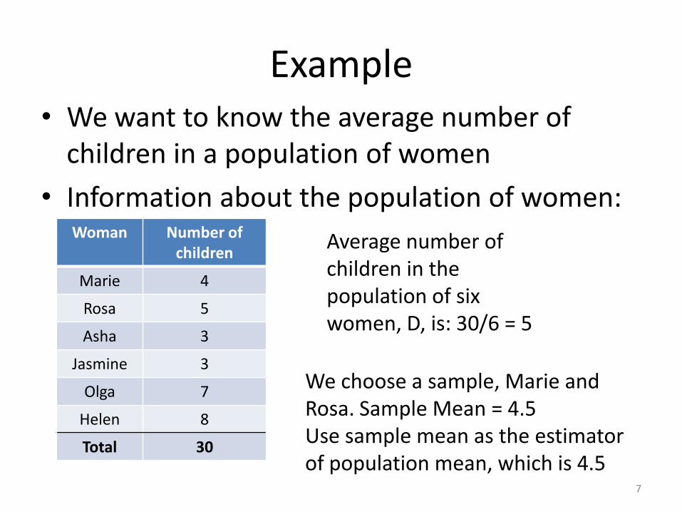
Sampling Error• When we draw just one sample, the population
estimate could be very close or very far from the population parameter
• Sampling error is a measure of how good a sample statistic is as an estimator of a population parameter
Sampling error is 0 for censuses (trivial)or for sample surveys if the population units are all the same
8
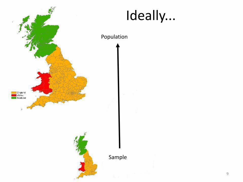
Ideally...Population
Sample
9

10
But if the sample is...
Sample
How do we compute the sampling error?
• From properties of the sampling distribution and the population
• Sampling distribution of an estimator of a population parameter is the distribution of the estimates of that population parameter under a particular sampling plan/sample design.
• Sampling plan: is “methodology used for selecting the sample from the population”
11

Sampling distribution of the estimator: the sample mean
12
True population mean
.35
.36
.37
.38
.39
.4
-.5 0 .5sample_mean
Pop. Mean

Woman Number of children
Marie 4
Rosa 5
Asha 3
Jasmine 3
Olga 7
Helen 8
Total 30
Sample No. Sample units
1 Marie, Rosa
2 Marie, Asha
3 Marie, Jasmine
4 Marie, Olga
5 Marie, Helen
6 Rosa, Asha
7 Rosa, Jasmine
8 Rosa, Olga
9 Rosa, Helen
10 Asha, Jasmine
11 Asha, Olga
12 Asha, Helen
13 Jasmine, Olga
14 Jasmine, Helen
15 Olga, Helen
Let us draw a sample of size 2.
All possible samples
13

Sample No.
Sample units Mean number of children in the sample (d)
1 Marie, Rosa (4+5)/2 = 4.5
2 Marie, Asha 3.5
3 Marie, Jasmine 3.5
4 Marie, Olga 5.5
5 Marie, Helen 6
6 Rosa, Asha 4
7 Rosa, Jasmine 4
8 Rosa, Olga 6
9 Rosa, Helen 6.5
10 Asha, Jasmine 3
11 Asha, Olga 5
12 Asha, Helen 5.5
13 Jasmine, Olga 5
14 Jasmine, Helen 5.5
15 Olga, Helen 7.5
The sample mean of a variable is an estimator of population mean of that variable.
E.g., if sample 1 were selected then the estimated number of children per woman in the population would be 4.5.
Note: The population mean is 5.
14

Sampling Distribution
Estimate of populationaverage number of
children (d)
Frequency Relative frequency(p)
3.0 1 1/15
3.5 2 2/15
4.0 2 2/15
4.5 1 1/15
5.0 2 1/15
5.5 3 3/15
6.0 2 2/15
6.5 1 1/15
7.5 1 1/15
15
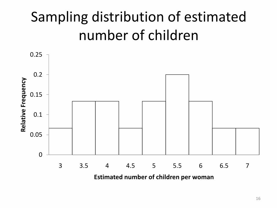
Sampling distribution of estimated number of children
0
0.05
0.1
0.15
0.2
0.25
3 3.5 4 4.5 5 5.5 6 6.5 7
Re
lati
ve F
req
ue
ncy
Estimated number of children per woman
16
Computing the Sampling Error(if you knew the population...)
• Take a population and draw all possible samples using a particular sampling technique (sampling plan)
• Compute the estimate of the population parameter for each sample
• Find out the frequency distribution of these estimates
• Compare the properties of the distribution with population parameters
17

Sampling Error (is one part of mean square error, MSE)
Two components
• Sampling Bias
• Standard Error/Sampling Variance
• Sampling Error = (Sampling Bias)2 + Sampling Variance
18
Sampling Bias
• Sampling Bias of an estimate of a population parameter = true value of the population parameter (typically unknown) MINUS the expected value/mean of the sampling distribution of the estimate.
• A measure of validity (if no measurement error)
19
Sampling variance & Standard error
• Sampling Variance of an estimator of a population parameter is the variance of the sampling distribution of that estimator
• Standard error = Square root of sampling variance
• SE is a measure of reliability (if no measurement error)
20

21
Sources of Error (Groves 1989)
Errors of Nonobservation
Sampling
Non-response
Coverage
Observational Errors
Interviewer
Respondent
Instrument
Coding
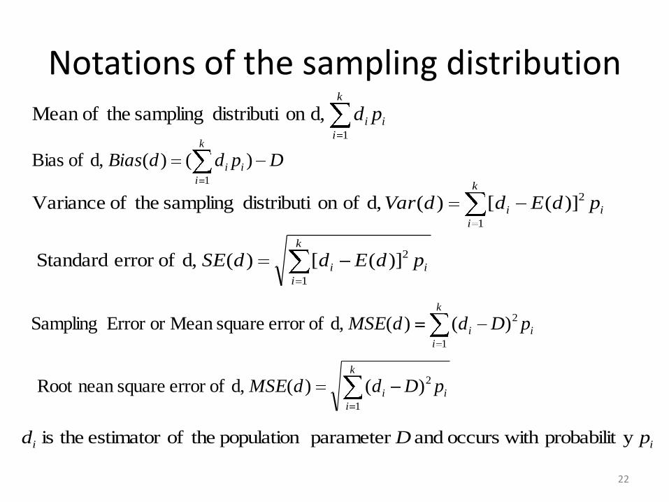
Notations of the sampling distribution
k
i
ii pdEddVar1
2)]([)( d, ofon distributi sampling theof Variance
k
i
ii pd1
d,on distributi sampling theofMean
k
i
ii pdEddSE1
2)]([)( d, oferror Standard
i
k
i
i pDddMSE1
2)()( d, oferror squareMean or Error Sampling
22
k
i
ii DpddBias1
)()( d, of Bias
ii pDd y probabilit with occurs and parameter population theofestimator theis
i
k
i
i pDddMSE1
2)()( d, oferror squarenean Root

Sampling Distribution
Estimate of populationaverage number of
children (d)
Frequency Relative frequency(p)
3.0 1 1/15
3.5 2 2/15
4.0 2 2/15
4.5 1 1/15
5.0 2 1/15
5.5 3 3/15
6.0 2 2/15
6.5 1 1/15
7.5 1 1/15
23

Computing bias, SE, MSE for our example
• Expected value of d = 5 which is equal to the true population parameter, D
• d is an unbiased estimator of D
• Variance of d = 1.47
• Standard error of d = 1.21
• MSE of d = 1.47 = Variance of d as d is an unbiased estimator of D
• RMSE of d = 1.21
24

Confidence interval at α(e.g., at 95%)
• CI at α is a range of the population parameter such that if we repeatedly sampled from the population then the probability that the true value of the population parameter will lie within that range is α
• Example: The population mean (=5) lies in the interval 4 and 6, 67% of times
• CI at 67% is (4,6)
25
Why probability samples?
• If we could draw all the possible samples (to get properties of the sampling distribution) and the population parameters then there would be no need to draw a sample!
• So how do we compute the Bias, SE, MSE?
Probability samples
26

Probability (random) Sampling
• “A probability sample has the characteristic that every element in the population has a known, nonzero probability of being included in the sample.” LL 1999
• This enables us to use its statistical properties to judge how good the estimators based on these samples are, i.e., compute Bias, SE, MSE
• Guards against selection bias
27

Probability (random) Sampling
• We will need a sampling frame: It is a list from which the sample can be selected and has the property that every population unit (member of the population) has some non-zero chance of being selected.
• But this list need not include every population unit, e.g., we are interested in the population of individuals residing in households and the sampling frame is a list of all households in UK
• Methodology or rule for choosing the sample: sampling design or sampling plan
28
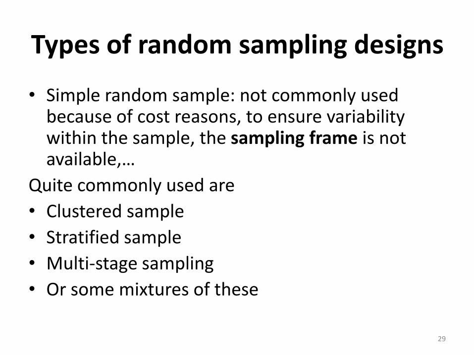
Types of random sampling designs
• Simple random sample: not commonly used because of cost reasons, to ensure variability within the sample, the sampling frame is not available,…
Quite commonly used are
• Clustered sample
• Stratified sample
• Multi-stage sampling
• Or some mixtures of these
29

Non-probability Samples
Cheaper, less time consuming
• Convenience sampling
• Purposive sampling
• Snowballing or respondent driven sampling
• Quota sampling
Cannot determine the statistical properties of the estimators based on these samples so cannot judge how good those estimators are
30

Example: Simple Random sample (SRS)
A simple random sample of n elements from a population of N elements is one in which each of the possible samples of n elements has the same probability of selection, namely 1/
• Each person has the same probability of being selected,
n
N
n
N
N
n
31
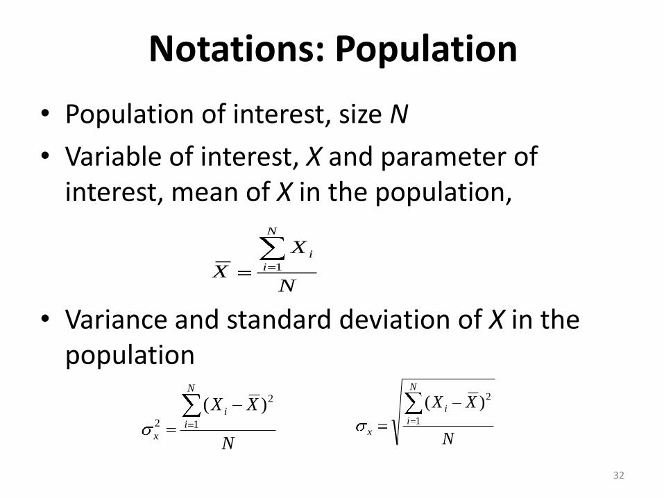
Notations: Population
• Population of interest, size N
• Variable of interest, X and parameter of interest, mean of X in the population,
• Variance and standard deviation of X in the population
N
X
X
N
i
i
1
N
XXN
i
i
x1
2
2
)(
N
XXN
i
i
x1
2)(
32

• A sample of size n is drawn, realizations of X in the sample are
• Sample mean
• Variance and standard deviation of x in the sample
n
i
ixn
x1
1
1
)(1
2
2
n
xx
s
n
i
i
x1
)(1
2
n
xx
s
n
i
i
x
nxxx ,..., 21
Notations: Sample
33
sample theof element ofselection ofy probabilit theis ipi
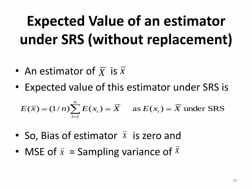
Expected Value of an estimator under SRS (without replacement)
• An estimator of is
• Expected value of this estimator under SRS is
• So, Bias of estimator is zero and
• MSE of = Sampling variance of
X x
34
x
x
SRSunder )( as )()/1()(1
XxEXxEnxE i
n
i
i
x
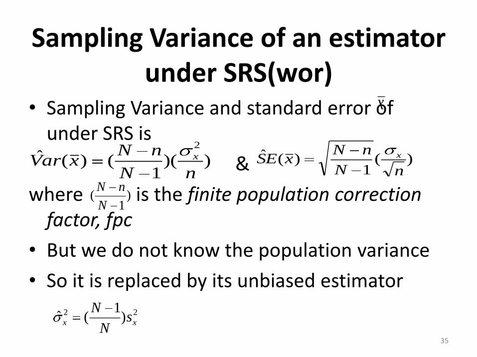
Sampling Variance of an estimator under SRS(wor)
• Sampling Variance and standard error of under SRS is
&
where is the finite population correction factor, fpc
• But we do not know the population variance
• So it is replaced by its unbiased estimator
))(1
()(ˆ2
nN
nNxarV x )(
1)(ˆ
nN
nNxES x
35
)1
(N
nN
x
22 )1
(ˆxx s
N
N

• fpc is close to 1 in most surveys (n<<<N)
• If fpc is ignored SE depends (positively) on population variance and (negatively) on sample size
• Note the difference between – standard deviation of X in the population
– estimate of the standard deviation of X,
– standard deviation of x in the sample
– standard error of the estimate of the mean of X,
xˆ
x
xs)(ˆ xES
))(()(ˆn
s
N
nNxES x
36
Other sample designs
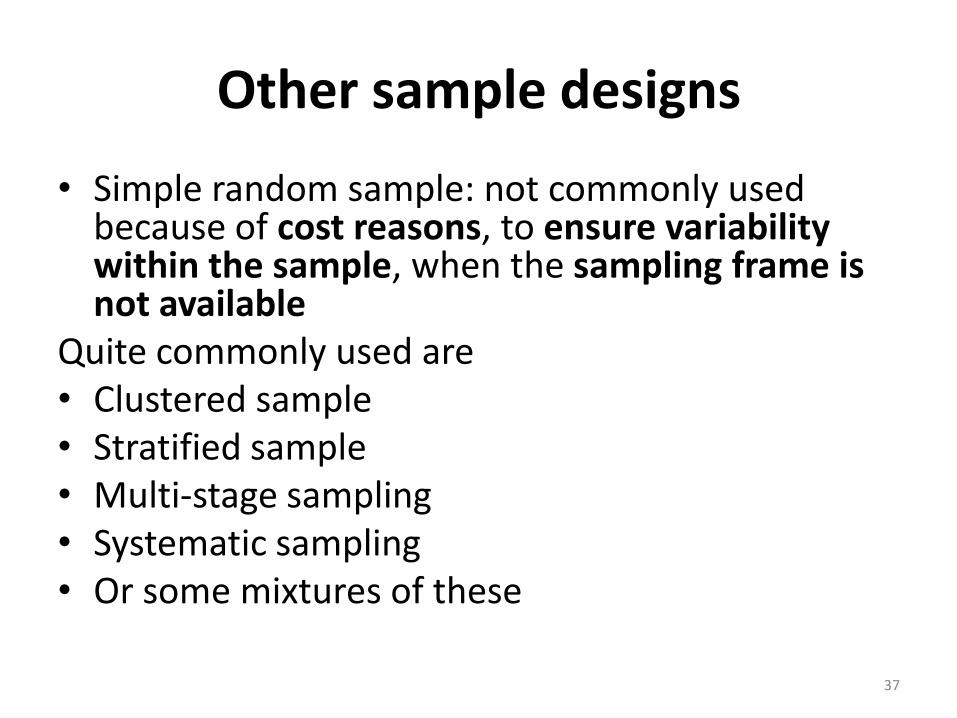
• Simple random sample: not commonly used because of cost reasons, to ensure variability within the sample, when the sampling frame is not available
Quite commonly used are• Clustered sample• Stratified sample• Multi-stage sampling• Systematic sampling• Or some mixtures of these
37

Cluster sampling
• Clusters: groups of population units, e.g., postcode sectors, schools, firms
• Clusters are selected instead of population units and then population units are selected within those clusters
• What are the advantages? – Frame of all population units not available, but
frame of clusters available
– Geographical clusters reduce interviewer costs
– Easier to access, e.g., students via schools38
One and multi-stage cluster sampling
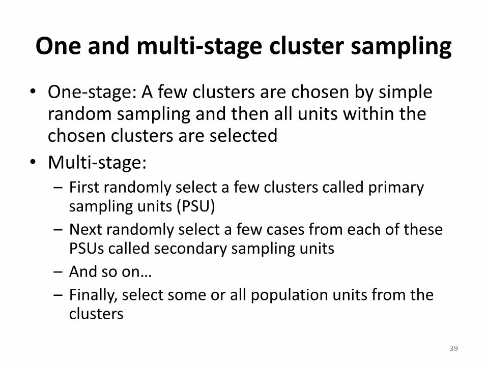
• One-stage: A few clusters are chosen by simple random sampling and then all units within the chosen clusters are selected
• Multi-stage: – First randomly select a few clusters called primary
sampling units (PSU)
– Next randomly select a few cases from each of these PSUs called secondary sampling units
– And so on…
– Finally, select some or all population units from the clusters
39
Stratified random sampling
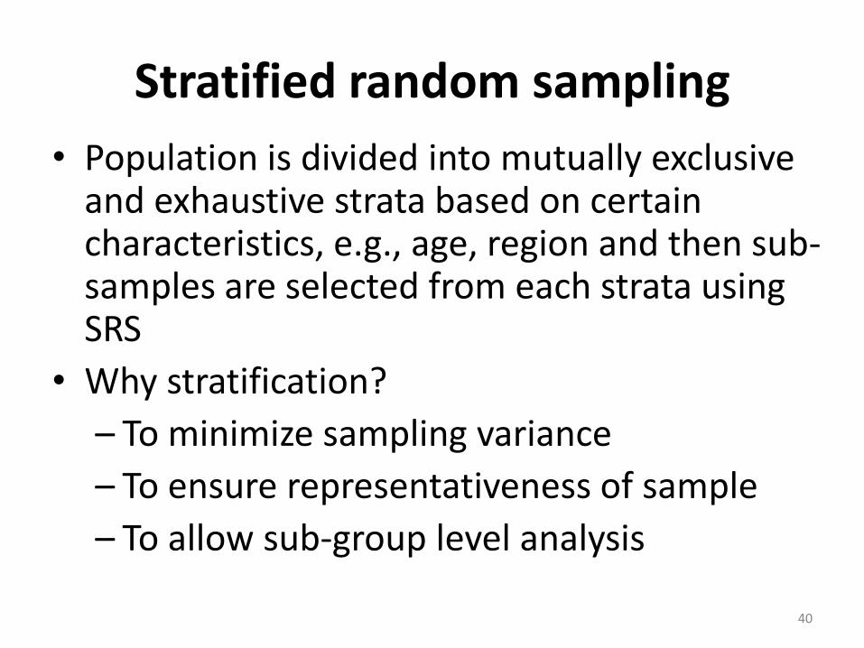
• Population is divided into mutually exclusive and exhaustive strata based on certain characteristics, e.g., age, region and then sub-samples are selected from each strata using SRS
• Why stratification?
– To minimize sampling variance
– To ensure representativeness of sample
– To allow sub-group level analysis
40

How to choose stratification variables?
Sampling variance depends only on within strata variance
– To minimize estimated variance of variable of interest, say wages
– We need to reduce within strata variance in terms of wages.
– As wages is not observed apriori, we need to choose a stratification variable say region, such that wages is highly correlated with region
41
How to choose stratification variables?
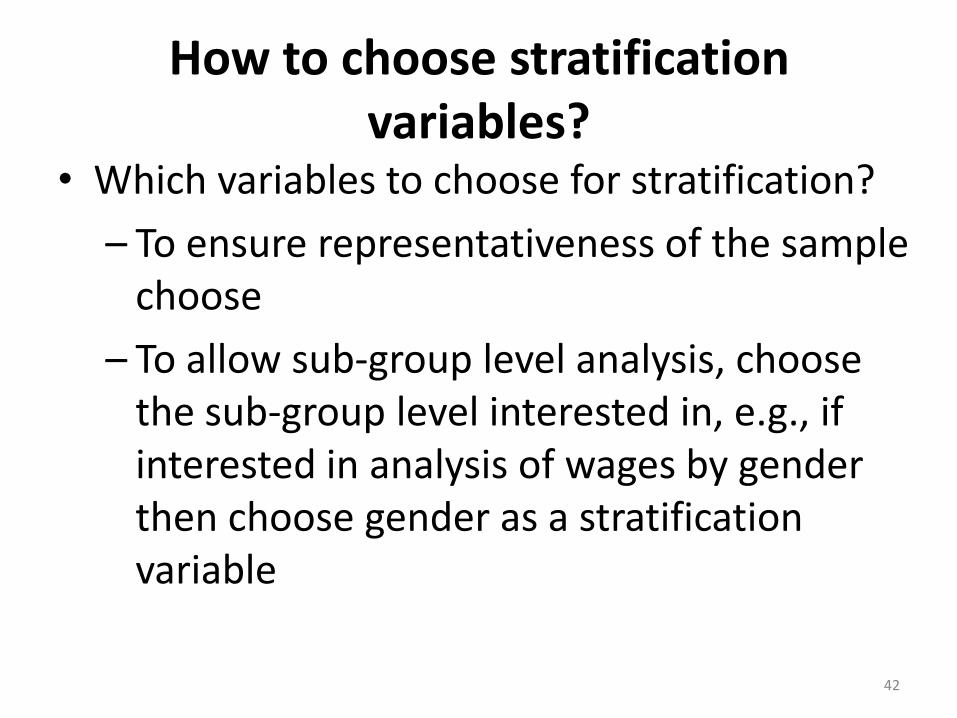
• Which variables to choose for stratification?
– To ensure representativeness of the sample choose
– To allow sub-group level analysis, choose the sub-group level interested in, e.g., if interested in analysis of wages by gender then choose gender as a stratification variable
42

Equal Probability Systematic Sampling
• Every kth unit is chosen where k, the sampling interval is the largest integer of N/n where (N: pop. Size, n: sample size)
• Start from a randomly selected unit within x1,…xk
• Useful when sampling frame is not known
• Only k possible samples
43

Equal Probability Systematic Sampling
• If k is an integer bias=0
• If k is not an integer, small bias. Modified method for unbiased estimates
• Variance is small if the units are completely randomly ordered w.r.t variable of interest
44

Variable Selection Fractions or Unequal Selection Probabilities
Sampling bias, unbiased estimators and weights
45

Variable Selection Fractions or Unequal Selection Probabilities
• Every population unit may not have the same selection probability (except in SRS)
• If those with different selection probabilities differ systematically from each other in terms of some variable, say wages, then we will get biased estimates of the population parameter, say, mean wages
• Think in terms of a stratified sample
46

VSF
47
Population units in this stratum = 100Sample units in this stratum = 10 Population units in
this stratum = 200Sample units in this stratum = 10
Population units in this stratum = 100Sample units in this stratum = 20

VSF
48
Selection probability or sampling fraction= 0.1 Selection
probability or sampling fraction = 0.05
Selection probability or sampling fraction = 0.2

VSF & biased estimators
49
condition this violatesVSF
fraction) sampling (equal allfor if )(
)()(
then stratain size sample
theis and stratain ofmean theis , stratain unit
offraction samplingor y probabilitselection theis N
n If
1
h
h
hN
n
N
nXxE
Xn
nxE
h
nhXXhi
h
h
h
n
h
h
hh
h

VSF & weights
50
Selection probability = 0.1Weights = 10
Selection probability = 0.05Weight = 20
Selection probability = 0.2Weight =5
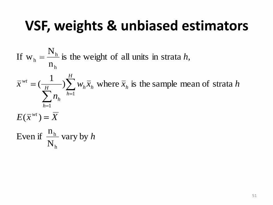
VSF, weights & unbiased estimators
51
h
XxE
hxxw
n
x
h
wt
h
H
h
hhH
h
h
wt
by vary N
n ifEven
)(
strata ofmean sample theis where)1
(
, stratain units all of weight theis n
N wIf
h
h
1
1
h
hh
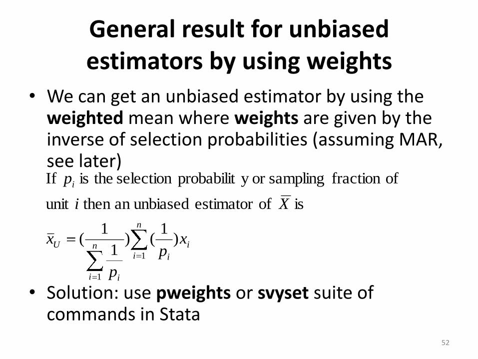
General result for unbiased estimators by using weights
• We can get an unbiased estimator by using the weighted mean where weights are given by the inverse of selection probabilities (assuming MAR, see later)
• Solution: use pweights or svyset suite of commands in Stata
52
i
n
i i
n
i i
U
i
xp
p
x
Xi
p
)1
()1
1(
is ofestimator unbiasedan then unit
offraction samplingor y probabilitselection theis If
1
1

Clustering, stratification
Sampling variance, design effect, correct standard errors
53
Design Effects, Effective sample size
• How do these sampling designs compare with SRS of equal size?
• Design effect, DEFF = Sampling Variance under complex sampling design/ Sampling Variance under SRS for samples of the same size
• Design factor, DEFT= Standard error under complex sampling design/ Standard error under SRS for samples of the same size
54
Design Effects, Effective sample size
• DEFF is not unique for each sample design although strongly affected by it
• DEFF varies by sample design, the variable of interest and the estimator
• Effective sample size, NEFF = Sample size required for a sample to produce the same sampling variance as a SRS
• Statistical softwares assume SRS
• Solution: use svyset suite of commands in Stata
55

DEFF for cluster sampling
56
1)1(1)(
sizecluster average theis andelation corr cluster -intra theis
)]1(1)[()(ˆ
)1
()
)1
(
1()(
PSU in SSU in element of prob.
selection theis )Pr()|Pr(),|Pr(
2
1 1 1
1 1 1
bxDEFF
b
bn
sxarV
xp
p
xE
kji
kkjkjip
uCLUSTER
xU
K
k
J
j
n
i
ijk
ijkK
k
J
j
n
i ijk
U
ththth
ijk
jk
jk
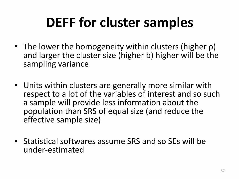
DEFF for cluster samples
• The lower the homogeneity within clusters (higher ρ) and larger the cluster size (higher b) higher will be the sampling variance
• Units within clusters are generally more similar with respect to a lot of the variables of interest and so such a sample will provide less information about the population than SRS of equal size (and reduce the effective sample size)
• Statistical softwares assume SRS and so SEs will be under-estimated
57
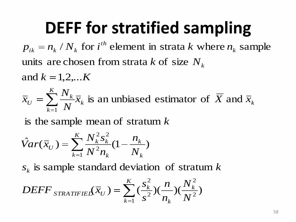
DEFF for stratified sampling
58
))()(()(
stratum ofdeviation standard sample is
)1()(ˆ
stratum ofmean sample theis
and ofestimator unbiasedan is
,...2,1 and
size of strata fromchosen are units
sample where stratain element for /
2
2
12
2
12
22
1
N
N
n
n
s
sxDEFF
ks
N
n
nN
sNxarV
k
xXxN
Nx
Kk
Nk
nkiNnp
k
k
K
k
kUSTRATIFIED
k
k
kK
k k
kkU
kk
K
k
kU
k
k
th
kkik

DEFF for stratified random samples
• DEFFSTRATIFIED(X)<1
– If units from different strata are different in terms of X
– If variance within strata are much smaller than overall variance (within strata variance is small & between strata variance is high)
• Statistical softwares assume SRS and so SEs will be over-estimated
59

Sources of Error
60

61
Sources of Error (Groves 1989)
Errors of Nonobservation
Sampling
Non-response
Coverage
Observational Errors
Interviewer
Respondent
Instrument
Coding

The survey process
62
Selecting the sample
Foot in the door
Interview
Coverage errorSampling error
Non-response error (locate-contact-interview)
Interviewer ErrorRespondent ErrorInstrument ErrorMode Error

Errors of nonobservation
• Sampling error
• Non-response error: Not every one selected into the sample takes part in the survey (unit non-response)
• Coverage error: The sample selected is such that some part of the population of interest had no chance of being selected
63

Unit Non-response
Eligible sample unit
Located
Contact
ParticipateRefuse to
participateUnable to participate
Non-contact
Not located
64
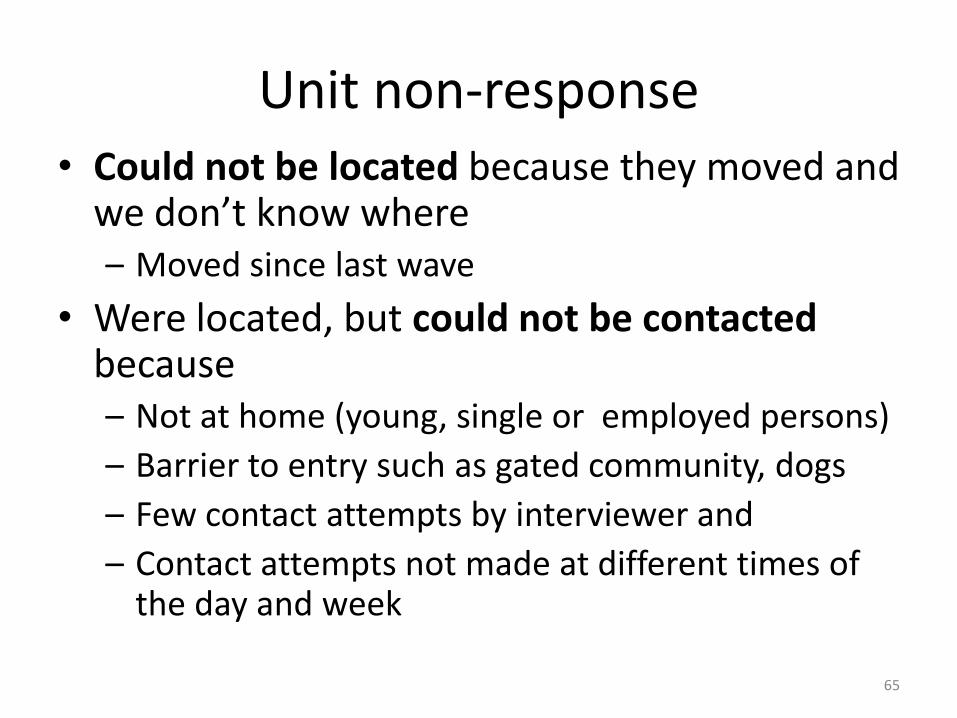
Unit non-response• Could not be located because they moved and
we don’t know where– Moved since last wave
• Were located, but could not be contacted because– Not at home (young, single or employed persons)
– Barrier to entry such as gated community, dogs
– Few contact attempts by interviewer and
– Contact attempts not made at different times of the day and week
65

Unit non-response• Could be contacted but refused to participate. This
could be because of – Security or confidentiality reasons– Not altruistic– Does not like inter-personal interactions– Time constraints, interview not worthwhile
• Could be contacted but unable to participate because of – Illness– Language problems
So, non-response is affected by the characteristics of the individual, the interviewer, survey topic, survey organization and also interview mode (Face-to-face, telephone, web, mail)
66

non-response Vs Ineligible• All those who are not in the population of
interest are considered to be ineligible
• In the BHPS all those living outside UK are considered to be ineligible or out-of-scope
• Compare this with non-respondents – they are eligible to be interviewed but could not be located, contacted or refused to participate
• This information is provided in the interview outcomes
67

Interview outcomes
Interview outcome
Full interview 500
Proxy interview 20
Refused to participate 20
Non-contact 60
Too ill 5
Language problems 5
Moved to outside UK 5
Unable to locate 5
68
response (ivfio)

Response rate
• Response rates - The number of complete interviews with reporting units divided by the number of eligible reporting units in the sample. [The American Association for Public Opinion Research. 2008. Standard Definitions: Final Dispositions
of Case Codes and Outcome Rates for Surveys. 5th edition. Lenexa,Kansas: AAPOR.]
• RR = Response units / Eligible sample units
• Different definitions for response rates –depends on how you deal with cases of unknown eligibility and how partial interviews are counted
69
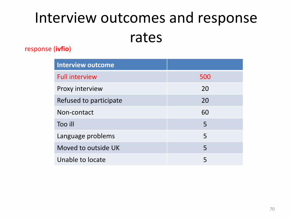
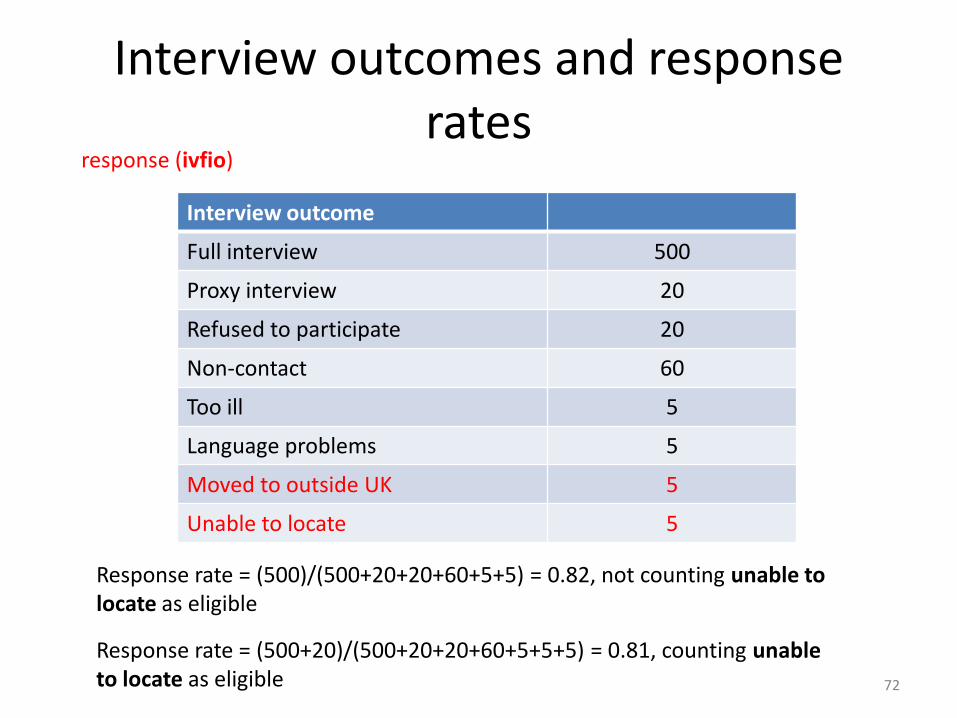
Interview outcomes and response rates
Interview outcome
Full interview 500
Proxy interview 20
Refused to participate 20
Non-contact 60
Too ill 5
Language problems 5
Moved to outside UK 5
Unable to locate 5
70
response (ivfio)

Interview outcomes and response rates
Interview outcome
Full interview 500
Proxy interview 20
Refused to participate 20
Non-contact 60
Too ill 5
Language problems 5
Moved to outside UK 5
Unable to locate 5
71
response (ivfio)
Interview outcomes and response rates
Interview outcome
Full interview 500
Proxy interview 20
Refused to participate 20
Non-contact 60
Too ill 5
Language problems 5
Moved to outside UK 5
Unable to locate 5
72
response (ivfio)
Response rate = (500)/(500+20+20+60+5+5) = 0.82, not counting unable to locate as eligible
Response rate = (500+20)/(500+20+20+60+5+5+5) = 0.81, counting unable to locate as eligible

73
Mean Square Error
(accuracy)
Variance
(precision)
Errors of Nonobservation
Coverage
Sampling
Non-response
Observational Errors
Interviewer
Respondent
Instrument
Mode
Bias
Errors of Nonobservation
Coverage
Sampling
Non-response
Observational Errors
Interviewer
Respondent
Instrument
Mode
Source: Robert M. Groves (1989) Survey Errors and Survey Costs, p.10

Mean square error
• Mean square error (MSE): is a measure of accuracy of the estimator as it is the mean squared deviations of the estimate from the true parameter value
• MSE = (Bias)2 + Variance
• Root mean square error (RMSE)
• If an estimator is unbiased then MSE = Variance
74
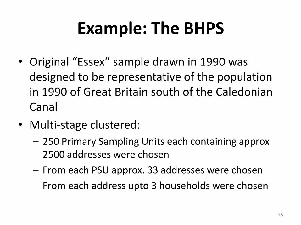
Example: The BHPS
• Original “Essex” sample drawn in 1990 was designed to be representative of the population in 1990 of Great Britain south of the Caledonian Canal
• Multi-stage clustered:
– 250 Primary Sampling Units each containing approx 2500 addresses were chosen
– From each PSU approx. 33 addresses were chosen
– From each address upto 3 households were chosen
75

Example: The BHPS
• Stratified by GOR regions, proportion of heads of households in professional or managerial positions proportion of pensionable age, metropolitan vs non-metropolitan areas
• (almost) Equal probability selection mechanism design
76

Example: The BHPS
• But at later waves additional samples from Scotland, Wales and Northern Ireland were added – with unequal selection probabilities
• Scotland and Wales added in 1999 and Northern Ireland added in 2001
• Survey design for Scotland and Wales samples was clustered and stratified – just as for the original Essex sample
77

Example: The BHPS
• Sample design for Northern Ireland sample was simple random sample
• wmemorig variable identifying the sample
• wmemorig is 1 for Original Essex sample
• wmemorig is 6 for Scottish sample
• wmemorig is 5 for Welsh sample
• wmemorig is 7 for Northern Ireland sample
78

79
Scotland is ‘over’ sampled
Each person living in Scotland has a much higher probability of being included in the BHPS than a person living in England
Example: BHPS sample members living in different countries in 1999
England n=12,566 (57%)
Scotland n=4,711 (21%)
Estimated UK population by region of residence in 1999 (National Statistics)
England N=49.75 m (84%)
Scotland N=5.12 m (9%)
But ...
Sample

Longitudinal non-response patternsExample: BHPS
80
Response type Wave
1 2 3 4 5 6 7 8 9
Full response R R R R R R R R R
Attrition 1 R
Attrition 2 R R R R R
Wave non-response R R R R R R R
• Wave non-response: When respondents do not participate in some of the waves
• Attrition: When respondents in panel studies drop out of the survey permanently
R: Response/interview adult

Example: The BHPS
• Estimate of UK wage will be biased if average wages in Scotland, Wales and Northern Ireland are different from that of England
• Estimate of UK wage will be biased if average wages or respondents are different from that of non-respondents
81

Weights? Think of VSF
• Those with lower probabilities of selection should have higher weights as they need to represent a larger number of units who are missing from the sample to produce unbiased estimates for the population of interest.
• Design weights are the inverse of selection probabilities
• Non-response weights are the inverse of response propensities/probability
82

How to choose weights?
• Most datasets provide different kinds of weights. To decide which weights to use
• Ask yourself what is your sample and which population are you interested in?
• To correct for unequal selection choose design weights
• To correct for non-response choose non-response weights
83
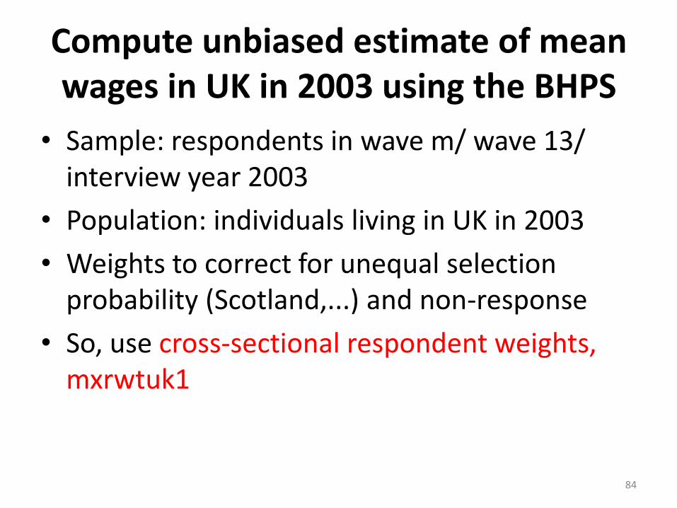
Compute unbiased estimate of mean wages in UK in 2003 using the BHPS
• Sample: respondents in wave m/ wave 13/ interview year 2003
• Population: individuals living in UK in 2003
• Weights to correct for unequal selection probability (Scotland,...) and non-response
• So, use cross-sectional respondent weights, mxrwtuk1
84

Compute unbiased estimate of standard errors of the estimates
Correct for clustering and stratification
• mpsu: variable identifying the primary sampling unit
• mstrata: variable identifying the strata
85
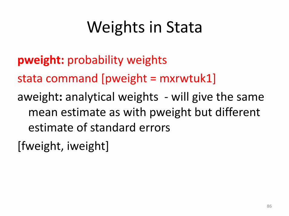
Weights in Stata
pweight: probability weights
stata command [pweight = mxrwtuk1]
aweight: analytical weights - will give the same mean estimate as with pweight but different estimate of standard errors
[fweight, iweight]
86

Accounting for complex survey design in Stata
Use svy suite of commands
• Tell Stata the details of the survey design
svyset pweight = mxrwtuk1 strata(mstrata) psu(mpsu)
• Next compute unbiased estimates & correct standard errors
svy: mean wage
svy: ci wage
svy: regress log(wage) education gender experience
87
Worksheet Part I
• Constructing sampling distributions
• Computing the sampling bias, sampling variance, sampling error
• Assume mean square error = sampling error
88

WorksheetPart II
• Compute estimates of mean wage in UK in 2003
—unweighted
—using weights
—using weights & correcting for sample design
—using both pweights and aweights
—using svy suite of commands
89

WorkseetPart II
• Compute and compare estimates of mean wage in different countries of UK in 2003
• How to account for Northern Ireland as it has a different sample design than the other samples
• Region of current residence is not identical to the sample origin – not all those currently living in Scotland were part of the Scottish sample
90

Variables used
• Dataset used: Week2Lecture1.dta• wage• xrwtuk1: cross-sectional respondent weights that
corrects for unequal selection probability, non-response, post stratification
• memorig: identifies the sample origin• strata: identifies the strata• psu: identifies the primary sampling unit• country: UK country currently living in• Week2Lecture1_Do&LogFiles.pdf• [Week2_data_prep_Do&LogFiles.pdf]
91

Week 2
Lecture 2
92

93
Mean Square Error
(accuracy)
Variance
(precision)
Errors of Nonobservation
Coverage
Sampling
Non-response
Observational Errors
Interviewer
Respondent
Instrument
Mode
Bias
Errors of Nonobservation
Coverage
Sampling
Non-response
Observational Errors
Interviewer
Respondent
Instrument
Mode
Source: Robert M. Groves (1989) Survey Errors and Survey Costs, p.10
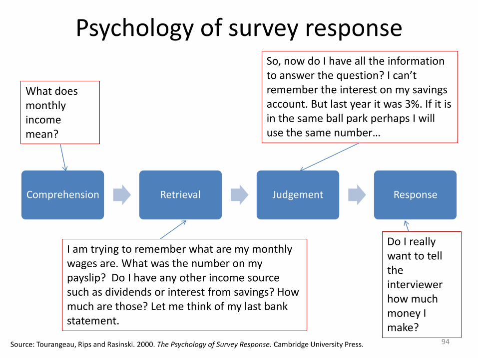
Psychology of survey response
94
Comprehension Retrieval Judgement Response
Source: Tourangeau, Rips and Rasinski. 2000. The Psychology of Survey Response. Cambridge University Press.
Do I really want to tell the interviewer how much money I make?
What does monthly income mean?
I am trying to remember what are my monthly wages are. What was the number on my payslip? Do I have any other income source such as dividends or interest from savings? How much are those? Let me think of my last bank statement.
So, now do I have all the information to answer the question? I can’t remember the interest on my savings account. But last year it was 3%. If it is in the same ball park perhaps I will use the same number…

Observational Errorsor Measurement Error
(not covered in this course)
• Data quality: Was the question answered correctly? Item non-response is an extreme case
• Respondent
• Interviewer
• Mode
• Instrument
95
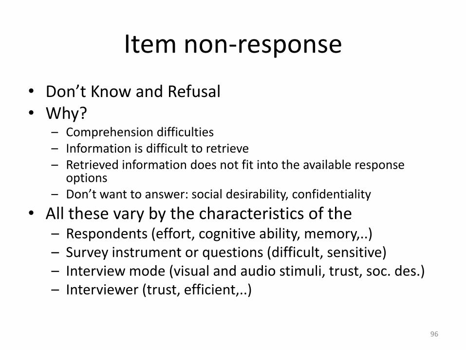
Item non-response
• Don’t Know and Refusal• Why?
– Comprehension difficulties– Information is difficult to retrieve– Retrieved information does not fit into the available response
options– Don’t want to answer: social desirability, confidentiality
• All these vary by the characteristics of the– Respondents (effort, cognitive ability, memory,..)– Survey instrument or questions (difficult, sensitive)– Interview mode (visual and audio stimuli, trust, soc. des.)– Interviewer (trust, efficient,..)
96

Errors of non-observation or issues of missing data?
97

Errors of non-observation/ Missing Data
• Unit non-response, item non-response, coverage error
• Some data will always be missing no matter how well the survey is done, e.g., wages of those who are not employed
• Some data will be missing because respondent is dead: No longer part of the population of interest and so not asked, e.g., health status of smokers who die during the course of the study
98

Missing DataXY *
vXZR*
0if 0
0 if 1
otherwise .
0if*
***
R
RR
RYY
99
Typology initially developed by Rubin (1976)
MCAR: Missing Completely At Random MAR: Missing At RandomNMAR: Not Missing At Random
observed is Y that phenomenon theis
observed be willY if determines which iablelatent var theis
interest of variableobserved theis interest, of iablelatent var theis
*
*
R
R
YY
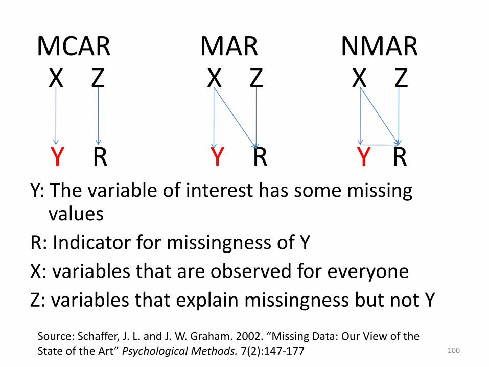
MCAR MAR NMARX Z X Z X Z
Y R Y R Y RY: The variable of interest has some missing
values
R: Indicator for missingness of Y
X: variables that are observed for everyone
Z: variables that explain missingness but not Y
100
Source: Schaffer, J. L. and J. W. Graham. 2002. “Missing Data: Our View of the State of the Art” Psychological Methods. 7(2):147-177

MCAR
• Missing Completely at Random (MCAR): The phenomenon of missing data is not affected by any observable or unobservable factors
• Example: Variable of interest is monthly pay and because of a mistake a random part of the proposed sample was not sampled
• So, there is no reason to believe that those not in the sample are different from those sampled.
101

MCAR
correlatednot are and
*
*
ZR
XY
0if 0
0 if 1
otherwise .
0if*
***
R
RR
RYY
102
• Pr(R=1|Y*,X,Z)=Pr(R=1|Z)• No estimation bias
MAR
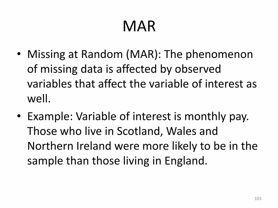
• Missing at Random (MAR): The phenomenon of missing data is affected by observed variables that affect the variable of interest as well.
• Example: Variable of interest is monthly pay. Those who live in Scotland, Wales and Northern Ireland were more likely to be in the sample than those living in England.
103

MAR
correlatednot are and
*
*
XZR
XY
0if 0
0 if 1
otherwise .
0if*
***
R
RR
RYY
104
• Pr(R=1|Y*,X,Z)=Pr(R=1|X,Z)• Estimation bias, if interested in making predictions
about Y*
• Solution: Weighting or imputation[In terms of our example: Y is monthly pay, R is 1 if the
person is selected into the sample and Z is region]

NMAR
• Not Missing at Random (NMAR): The phenomenon of missing data is affected by all values (missing or otherwise) of the variable of interest and other observable & unobservable factors
• Example: Variable of interest is women’s monthly pay, those who are not employed do not have a monthly pay and are likely to be different from women who are employed in terms of “unobserved” factors
105

Example: women’s earnings model
– Women with young children have higher reservation wages (childcare, utility from raising children)
– Women with young children who do participate do so because of some qualities that are rewarded highly in the labour market resulting in higher wage offers than other women
– These women are a non-random sub-sample of all women with young children
– These qualities are unobserved
106

NMAR
correlated are and
*
*
XZR
XY
0if 0
0 if 1
otherwise .
0if*
***
R
RR
RYY
107
• Pr(R=1|Y*,X,Z)=Pr(R=1|Y*-Xβ,X,Z)= Pr(R=1|ε,X,Z)• Estimation Bias, if interested in making
predictions about Y*
• Solution: Heckman selection

Correcting for selection bias: Heckman Two-stage
and of valuesestimated ofFunction a is
Ratio sMill' Inverse asprobit usingby and
estimatingby Ratio sMill' Inverse computefirst But
Ratio sMill' Inverse Re
:Solution sHeckman'
normal bivariate as ddistribute and :Assumption
0 if 0
0 if 1
0 if .
1 if
*
*
**
*
*
errortermsXYgress
R
RR
R
RYY
XZR
XY
108Heckman (1979), Vella (1998)
Correcting for selection bias: Heckman Two-stage
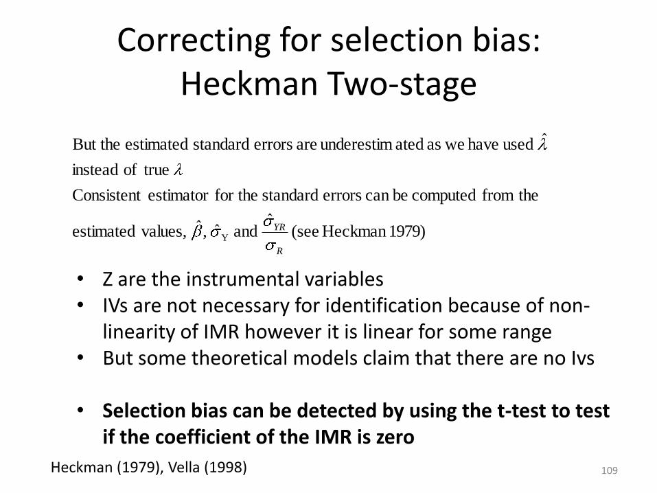
1979)Heckman (see ˆ
and ˆ ,ˆ values,estimated
thefrom computed becan errors standard for theestimator Consistent
trueof instead
ˆ used have weas atedunderestim are errors standard estimated But the
Y
R
YR
109
• Z are the instrumental variables• IVs are not necessary for identification because of non-
linearity of IMR however it is linear for some range• But some theoretical models claim that there are no Ivs
• Selection bias can be detected by using the t-test to test if the coefficient of the IMR is zero
Heckman (1979), Vella (1998)

Correcting for selection bias: MLE/Tobit type two
• Again assuming the error terms in the two equations are distributed jointly as bivariate normal then β can be consistently estimated using MLE (see Vella 1998)
• Advantage: most efficient under the assumption of joint normality of the two error terms
• Disadvantage: the maximization process may not converge
110
Heckman, MLE/Tobit type two in Stata
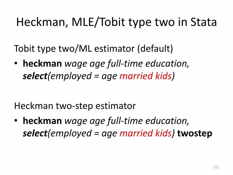
Tobit type two/ML estimator (default)
• heckman wage age full-time education, select(employed = age married kids)
Heckman two-step estimator
• heckman wage age full-time education, select(employed = age married kids) twostep
111

Weighted estimation
),0( 2* Niidxy
)1,0(* Niidvwherevzd
missing is if0if 0
observed is if 0if1
otherwise .
0if**
****
yd
ydd
dyy
)()|1Pr()|0*Pr(
of inverse by thegiven are Weights
zzdzd
z)x,|1Pr(dz)x,y*,|1Pr(d
variablesobservedgiven d oft independen *y
:(CIA) assumption ceindependen lconditionaor
(MAR) randomat missing of Assumption
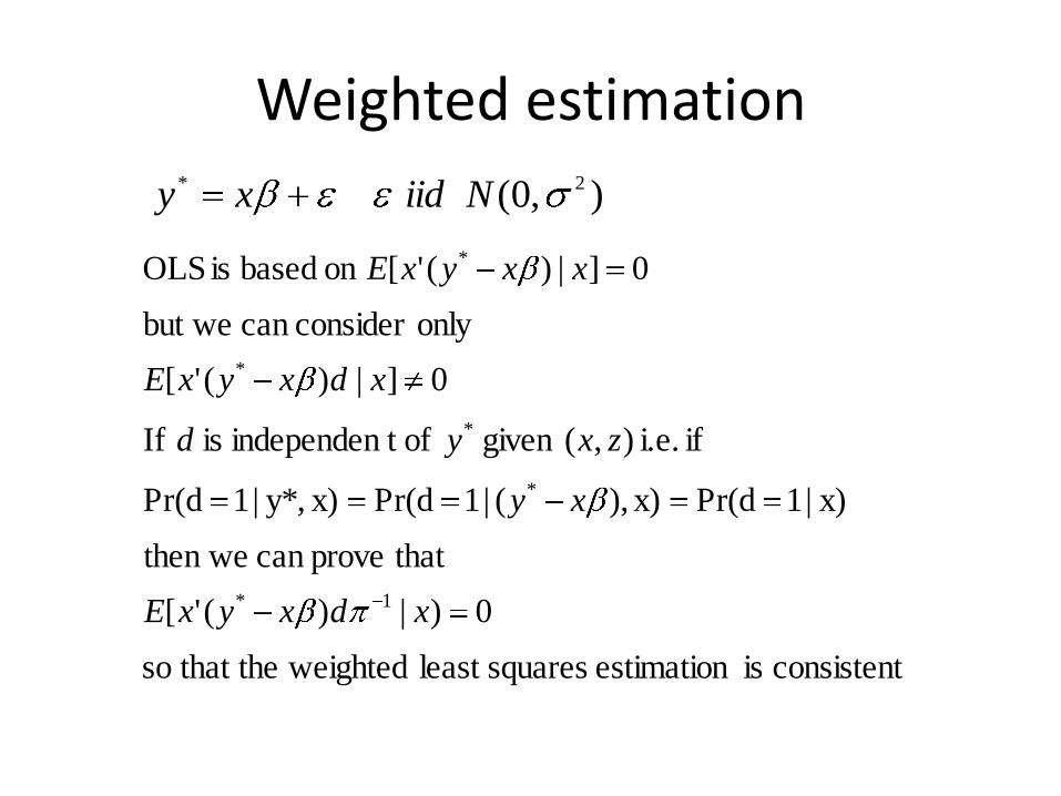
Weighted estimation
),0( 2* Niidxy
consistent is estimation squaresleast weighted that theso
0)|)('[
that provecan then we
x)|1Pr(dx),)( |1Pr(dx)y*, |1Pr(d
if i.e. ),(given oft independen is If
0]|)('[
onlyconsider can but we
0]|)('[on based is OLS
1*
*
*
*
*
xdxyxE
xy
zxyd
xdxyxE
xxyxE
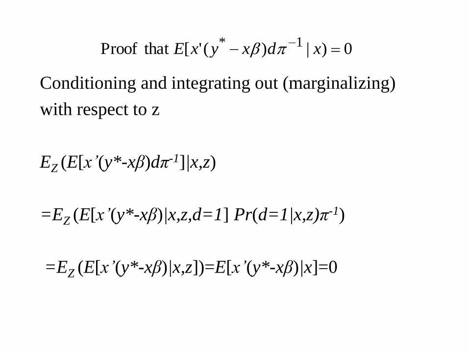
Conditioning and integrating out (marginalizing)
with respect to z
EZ (E[x’(y*-xβ)dπ-1]|x,z)
=EZ (E[x’(y*-xβ)|x,z,d=1] Pr(d=1|x,z)π-1)
=EZ (E[x’(y*-xβ)|x,z])=E[x’(y*-xβ)|x]=0
0)|)('[ that Proof 1* xdxyxE

Creating design & non-response weights
otherwise 0
0 if 1Re
as modelled becan behavior Response
*
*
Rsponse
ZR
115
• Estimate probability of response by probit or logit• Compute the non-response weight as the inverse of
the estimated probability of response (There are other methods to compute non-response weight)
i
i
i
pwii
p
1 is unit for ght design wei then unit
offraction samplingor y probabilitselection theis If
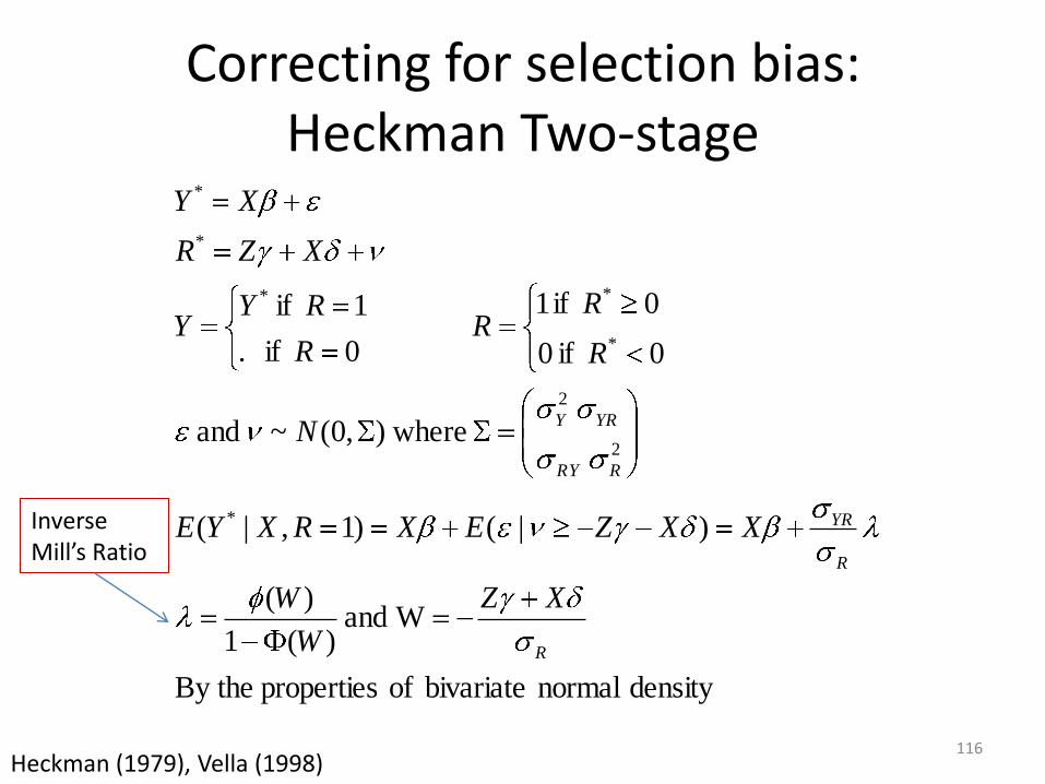
Correcting for selection bias: Heckman Two-stage
density normal bivariate of properties By the
Wand )(1
)(
)|()1,|(
where),0(~ and
0 if 0
0 if 1
0 if .
1 if
*
2
2
*
**
*
*
R
R
YR
RRY
YRY
XZ
W
W
XXZEXRXYE
N
R
RR
R
RYY
XZR
XY
116
Inverse Mill’s Ratio
Heckman (1979), Vella (1998)

Correcting for selection bias: Heckman Two-stage
0),,|(),,|(
),,|(),,|(
),,|()1,,|(
where
)1,|(
)()1,|(
So,
)1,|(
As
**
**
*
*
XZXEXZXE
XZXEXZXE
XZXERXE
RXYEY
RXYEY
XRXYE
XY
R
YR
R
YR
R
YR
R
YR
R
YR
R
YR
R
YR
117
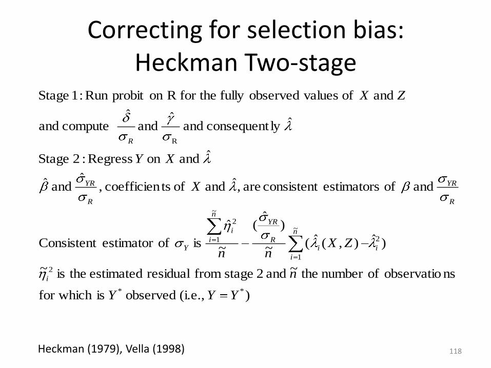
Correcting for selection bias: Heckman Two-stage
) (i.e., observed isfor which
nsobservatio ofnumber the~ and 2 stage from residual estimated theis ~
)ˆ),(ˆ(~
)ˆ
(
~
ˆ
is ofestimator Consistent
and of estimators consistent are ,ˆ and of tscoefficien ,ˆ
and ˆ
ˆ and on Regress :2 Stage
ˆly consequent and ˆ
andˆ
compute and
and of valuesobservedfully for the Ron probit Run :1 Stage
**
2
2
~
1
~
1
2
R
YYY
n
ZXnn
X
XY
ZX
i
i
n
i
iR
YRn
i
i
Y
R
YR
R
YR
R
118Heckman (1979), Vella (1998)