Stat BootcampSession 2-2

Professor P. K. Kannan1

Agenda

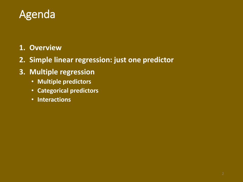
1. Overview2. Simple linear regression: just one predictor3. Multiple regression

• Multiple predictors• Categorical predictors • Interactions

2

Part I: Overview

3

Steps before modeling

• Again, eyeball your data • Ask yourself the following questions

• What is the unit of observation • Which variable is my dependent variable: the variable that we are

interested in explaining or predicting • Which variables are my independent variables (predictors)• What is the measurement type for each of the variables

• Categorical?• Continuous?

• Use the flowchart on the next page

4

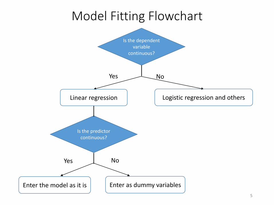
Model Fitting Flowchart

5

Is the dependent variable

continuous?

Yes No

Linear regression Logistic regression and others

Is the predictor continuous?

Yes No

Enter as dummy variablesEnter the model as it is

Part II: Simple Linear Regression

using the Airline.xlsx data

6

Roadmap

• Correlation: Pearson correlation

• Scatterplot

• Simple linear regression • Model specification • Coefficients interpretation • Overall goodness-of-fit of the model

7

• Correlation measures the strength and direction of the relationship between two continuous variables

• Direction • r → 0: X and Y are not linearly related• r → +1: X and Y have perfectly positive linear relation• r → -1: X and Y have perfectly negative linear relation

• Strength• Determined by the absolute value of r• The general guideline of effect size for r:

• But the thresholds may vary by applications—you should let your business application determine what is considered a strong correlation

8

Pearson correlation coefficient

Effect size r

Small 0.1

Medium 0.3

Large 0.5

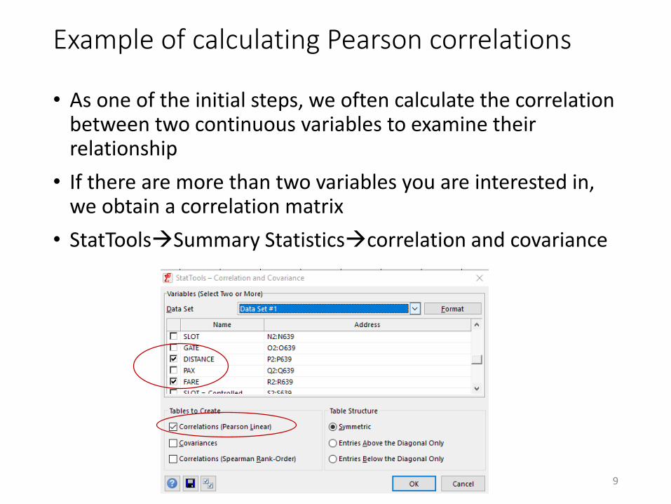
Example of calculating Pearson correlations

• As one of the initial steps, we often calculate the correlation between two continuous variables to examine their relationship

• If there are more than two variables you are interested in, we obtain a correlation matrix

• StatToolsSummary Statisticscorrelation and covariance

9

• A correlation matrix is symmetrical around the diagonal• Each entry is the Pearson correlation between the row

variable and the column variable • 0.670 = the Pearson correlation between fare (the row variable) and

distance (the column variable)

• Interpretation• 0.670>0: the correlation is positive• 0.670 indicates strong correlation • So, if we do a scatterplot between fare and distance, what kind of

plot do we expect to see?

10

Scatterplot between fare and distance

• StatToolsSummary GraphsScatterplot

11

• As expected, we see a positive and strong relationship in the plot.

• But a correlation or a scatterplot cannot do prediction. So, we need a model.

• A linear relationship seems appropriate here let’s fit a linear regression model

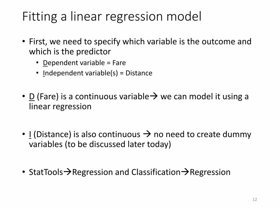
Fitting a linear regression model

• First, we need to specify which variable is the outcome and which is the predictor

• Dependent variable = Fare• Independent variable(s) = Distance

• D (Fare) is a continuous variable we can model it using a linear regression

• I (Distance) is also continuous no need to create dummy variables (to be discussed later today)

• StatToolsRegression and ClassificationRegression

12

•

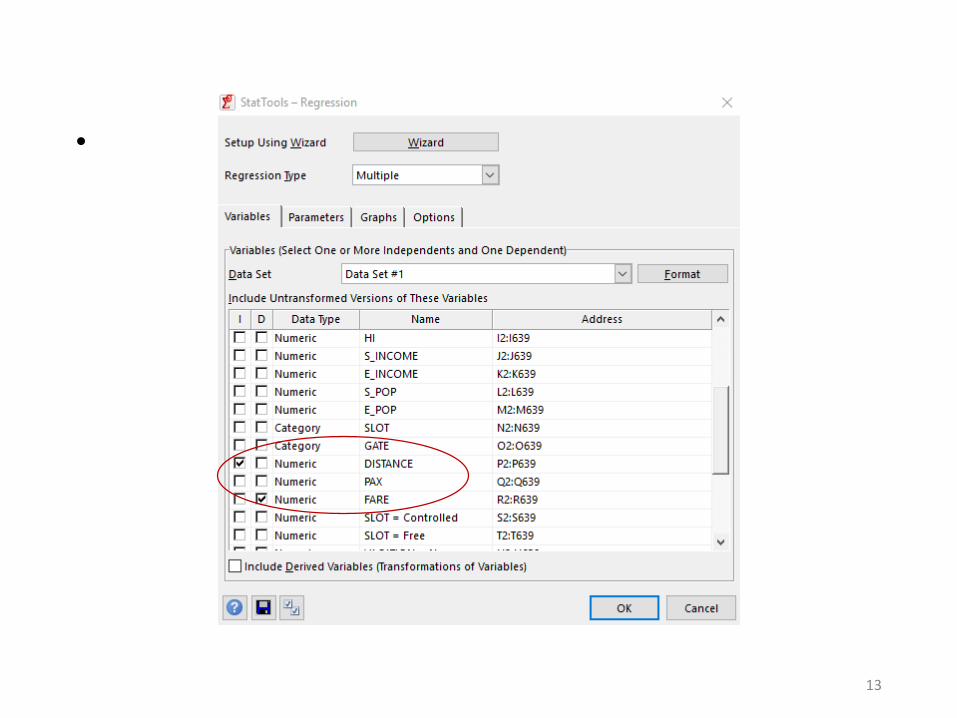
13

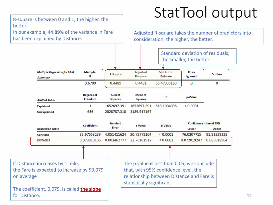
StatTool output

14

R-square is between 0 and 1; the higher, the better. In our example, 44.89% of the variance in Fare has been explained by Distance.

Adjusted R-square takes the number of predictors into consideration; the higher, the better.

Standard deviation of residuals; the smaller, the better

If Distance increases by 1 mile,the Fare is expected to increase by $0.079 on average

The coefficient, 0.079, is called the slopefor Distance.

The p value is less than 0.05, we conclude that, with 95% confidence level, the relationship between Distance and Fare is statistically significant

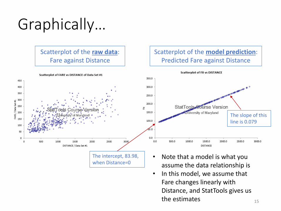
Graphically…

15

Scatterplot of the raw data: Fare against Distance

Scatterplot of the model prediction: Predicted Fare against Distance

The intercept, 83.98, when Distance=0

The slope of this line is 0.079

• Note that a model is what you assume the data relationship is

• In this model, we assume that Fare changes linearly with Distance, and StatTools gives us the estimates

Part III: Multiple Regression

16

• Multiple predictors

• Categorical variables

• Interactions

Linear regression with multiple predictors• Now, let’s expand our model to include three predictors:

coupon, distance, and Pax𝐹𝐹𝐹𝐹𝐹𝐹𝐹𝐹 = 𝐼𝐼𝐼𝐼𝐼𝐼𝐹𝐹𝐹𝐹𝐼𝐼𝐹𝐹𝐼𝐼𝐼𝐼 + 𝑏𝑏1𝐶𝐶𝐶𝐶𝐶𝐶𝐼𝐼𝐶𝐶𝐼𝐼+𝑏𝑏2𝐷𝐷𝐷𝐷𝐷𝐷𝐼𝐼𝐹𝐹𝐼𝐼𝐼𝐼𝐹𝐹+𝑏𝑏3𝑃𝑃𝐹𝐹𝑃𝑃 + e

17

The adjusted R-square is smaller than the previous one, 0.4481, suggesting that the two added variables are not predictive of Fare

The p-values for Coupon and Pax are greater than 0.05, indicating that, after controlling for other variables, neither is a significant predictor for Fare (in other words, the coefficient for Coupon or Pax is not statistically different from zero)

Prediction

• Using the estimated coefficients, we can now write the prediction equation:

• What is the predicted average fare for a route of 2,000 miles, with an average number of coupons of 1.5, and the number of passengers being 6,500?

18

𝐹𝐹𝐹𝐹𝐹𝐹𝐹𝐹 = 95.81 − 9.62 ∗ 𝐶𝐶𝐶𝐶𝐶𝐶𝐼𝐼𝐶𝐶𝐼𝐼+0.08 ∗ 𝐷𝐷𝐷𝐷𝐷𝐷𝐼𝐼𝐹𝐹𝐼𝐼𝐼𝐼𝐹𝐹-0.0017 ∗ 𝑃𝑃𝐹𝐹𝑃𝑃

𝐹𝐹𝐹𝐹𝐹𝐹𝐹𝐹 = 95.81 − 9.62 ∗ 1.5+0.08 ∗ 2000-0.0017 ∗ 6500= $230.33

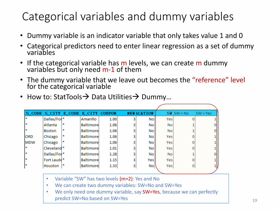
Categorical variables and dummy variables• Dummy variable is an indicator variable that only takes value 1 and 0• Categorical predictors need to enter linear regression as a set of dummy

variables• If the categorical variable has m levels, we can create m dummy

variables but only need m-1 of them• The dummy variable that we leave out becomes the “reference” level

for the categorical variable• How to: StatTools Data Utilities Dummy…

19

• Variable “SW” has two levels (m=2): Yes and No• We can create two dummy variables: SW=No and SW=Yes• We only need one dummy variable, say SW=Yes, because we can perfectly

predict SW=No based on SW=Yes

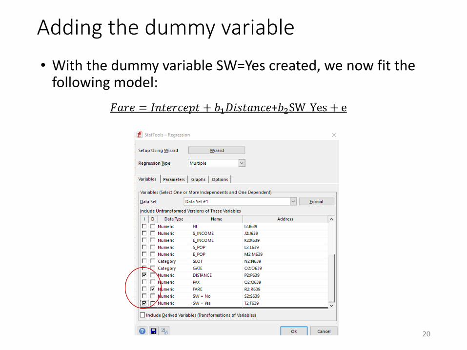
Adding the dummy variable

• With the dummy variable SW=Yes created, we now fit the following model:

20

𝐹𝐹𝐹𝐹𝐹𝐹𝐹𝐹 = 𝐼𝐼𝐼𝐼𝐼𝐼𝐹𝐹𝐹𝐹𝐼𝐼𝐹𝐹𝐼𝐼𝐼𝐼 + 𝑏𝑏1𝐷𝐷𝐷𝐷𝐷𝐷𝐼𝐼𝐹𝐹𝐼𝐼𝐼𝐼𝐹𝐹+𝑏𝑏2SW_Yes + e

StatToolsoutput

21

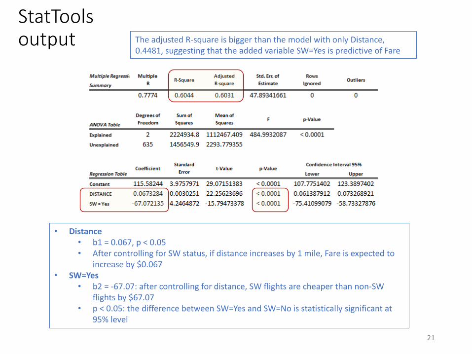
The adjusted R-square is bigger than the model with only Distance, 0.4481, suggesting that the added variable SW=Yes is predictive of Fare

• Distance• b1 = 0.067, p < 0.05• After controlling for SW status, if distance increases by 1 mile, Fare is expected to

increase by $0.067• SW=Yes

• b2 = -67.07: after controlling for distance, SW flights are cheaper than non-SW flights by $67.07

• p < 0.05: the difference between SW=Yes and SW=No is statistically significant at 95% level

Interactions between predictors

• In the previous example, we fit this model:

• By setting the model as above, we assume that the slope for Distance is the same between SW flights and non-SW flights

• How do we know? Because there is only one slope for Distance specified in the regression

• We might want to answer this question: is there a different relationship between Distance and Fare for SW flights?

• To answer this question, we need to have a separate slope for Distance for SW flights and another slope for non-SW slights

• We do so by adding a Distance X SW_Yes interaction into the model

22

𝐹𝐹𝐹𝐹𝐹𝐹𝐹𝐹 = 𝐼𝐼𝐼𝐼𝐼𝐼𝐹𝐹𝐹𝐹𝐼𝐼𝐹𝐹𝐼𝐼𝐼𝐼 + 𝑏𝑏1𝐷𝐷𝐷𝐷𝐷𝐷𝐼𝐼𝐹𝐹𝐼𝐼𝐼𝐼𝐹𝐹+𝑏𝑏2SW_Yes + e

𝐹𝐹𝐹𝐹𝐹𝐹𝐹𝐹 = 𝐼𝐼𝐼𝐼𝐼𝐼𝐹𝐹𝐹𝐹𝐼𝐼𝐹𝐹𝐼𝐼𝐼𝐼 + 𝑏𝑏1𝐷𝐷𝐷𝐷𝐷𝐷𝐼𝐼𝐹𝐹𝐼𝐼𝐼𝐼𝐹𝐹+𝑏𝑏2SW_Yes+𝑏𝑏3𝐷𝐷𝐷𝐷𝐷𝐷𝐼𝐼𝐹𝐹𝐼𝐼𝐼𝐼𝐹𝐹XSW_Yes + e

Adding an interaction to the model

• Steps: 1. Use StatToolsData Utilities Interactions to create an

interaction term between Distance and SW_Yes

2. The interaction is added as a new variable in the dataset, named “Interaction(Distance, SW=Yes)”

3. Add the new variable to regression model as a continuous variable in StatToolsRegression and classification

23

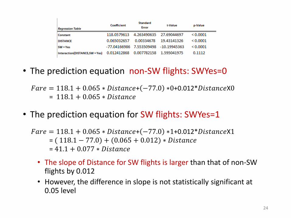
• The prediction equation non-SW flights: SWYes=0

• The prediction equation for SW flights: SWYes=1

• The slope of Distance for SW flights is larger than that of non-SW flights by 0.012

• However, the difference in slope is not statistically significant at 0.05 level

24

𝐹𝐹𝐹𝐹𝐹𝐹𝐹𝐹 = 118.1 + 0.065 ∗ 𝐷𝐷𝐷𝐷𝐷𝐷𝐼𝐼𝐹𝐹𝐼𝐼𝐼𝐼𝐹𝐹+ −77.0 ∗0+0.012*𝐷𝐷𝐷𝐷𝐷𝐷𝐼𝐼𝐹𝐹𝐼𝐼𝐼𝐼𝐹𝐹X0= 118.1 + 0.065 ∗ 𝐷𝐷𝐷𝐷𝐷𝐷𝐼𝐼𝐹𝐹𝐼𝐼𝐼𝐼𝐹𝐹

𝐹𝐹𝐹𝐹𝐹𝐹𝐹𝐹 = 118.1 + 0.065 ∗ 𝐷𝐷𝐷𝐷𝐷𝐷𝐼𝐼𝐹𝐹𝐼𝐼𝐼𝐼𝐹𝐹+ −77.0 ∗1+0.012*𝐷𝐷𝐷𝐷𝐷𝐷𝐼𝐼𝐹𝐹𝐼𝐼𝐼𝐼𝐹𝐹X1= ( 118.1 − 77.0) + (0.065 + 0.012) ∗ 𝐷𝐷𝐷𝐷𝐷𝐷𝐼𝐼𝐹𝐹𝐼𝐼𝐼𝐼𝐹𝐹= 41.1 + 0.077 ∗ 𝐷𝐷𝐷𝐷𝐷𝐷𝐼𝐼𝐹𝐹𝐼𝐼𝐼𝐼𝐹𝐹

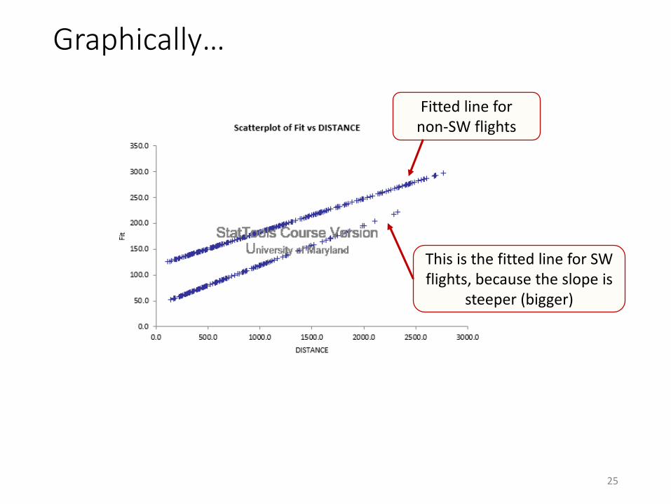
Graphically…

25

This is the fitted line for SW flights, because the slope is

steeper (bigger)

Fitted line for non-SW flights