Embed Size (px)
Citation preview

Preface
This documentation accompanies the WebCab Portfolio J2SE Component. The purposeof this documentation is to provide a clear and concise description of all aspects that arelikely to be encountered in real life applications by developers and users of this J2SE Com-ponent. WebCab Portfolio contains methods which use the Markowitz and Capital AssetPricing Model to construct a portfolio which for a given level of risk offers the greatestexpected return.
The first chapter of this documentation contains a brief introduction to the most im-portant implemented features and related system requirements. In chapter two we let thedeveloper quickly get started with deploying the component by detailing deployment tech-niques on the most widely used application servers. We also detail how the functionalityof this component can be tested through connecting to online web service demos hostedat J2SE Homepage. The third chapter contains the mathematical documentation, whichrepresents the theoretical background of this component’s implemented features. Chapterfour contains the programmer’s guide containing a road map for developers to take advan-tage of every feature and capability. In chapter five we provide some examples to illustratehow features detailed within the programmer’s guide can be applied in practice. Finally,we introduce WebCab Components, its philosophy and approach to serving the JavaTM
development community with robust and powerful J2SE Components.
If you have any suggestions for additional functionality, which we could include into futuredevelopment cycles or any other queries then please feel free to contact us via our supportforum at:
http://www.webcabcomponents.com/support/index.php
Good luck with your project and thank you for your interest in our components.
The WebCab Components Team
i

Contents
Preface i
1 Introduction 11.1 Product Description . . . . . . . . . . . . . . . . . . . . . . . . . . . . . . 1
1.1.1 Overview . . . . . . . . . . . . . . . . . . . . . . . . . . . . . . . . 11.1.2 Details . . . . . . . . . . . . . . . . . . . . . . . . . . . . . . . . . . 1
1.2 Package Details . . . . . . . . . . . . . . . . . . . . . . . . . . . . . . . . . 31.3 Prerequisites and Compatibility . . . . . . . . . . . . . . . . . . . . . . . . 3
1.3.1 System Requirements . . . . . . . . . . . . . . . . . . . . . . . . . . 31.3.2 Compatibility . . . . . . . . . . . . . . . . . . . . . . . . . . . . . . 4
2 Where do I Start? 52.1 Using the J2SE JAR file . . . . . . . . . . . . . . . . . . . . . . . . . . . . 5
2.1.1 Compilation . . . . . . . . . . . . . . . . . . . . . . . . . . . . . . . 52.1.2 Packaging . . . . . . . . . . . . . . . . . . . . . . . . . . . . . . . . 6
3 Mathematical Documentation 103.1 Assumptions, Questions, Functionality and Problems . . . . . . . . . . . . 10
3.1.1 Assumptions of Markowitz Theory . . . . . . . . . . . . . . . . . . 103.1.2 Assumptions of Capital Asset Pricing Model (CAPM) . . . . . . . . 113.1.3 What problems do these Models address . . . . . . . . . . . . . . . 113.1.4 Range of Functionality contained within the :services: . . . . . . . . 123.1.5 Problems with the Application of the Markowitz Theory and CAPM 13
3.2 Preliminaries and Auxiliary class’s . . . . . . . . . . . . . . . . . . . . . . . 163.2.1 Choices in Approach and other issues . . . . . . . . . . . . . . . . . 163.2.2 Basic Formulae for the Return, Covariance, Correlation and Risk . 17
3.3 Expected Return and Risk from a Portfolio with two Assets . . . . . . . . 213.3.1 Motivation . . . . . . . . . . . . . . . . . . . . . . . . . . . . . . . . 213.3.2 Formulation for a Portfolio of two assets . . . . . . . . . . . . . . . 223.3.3 Minimum risk of a portfolio with two assets . . . . . . . . . . . . . 22
3.4 Markowitz Theory . . . . . . . . . . . . . . . . . . . . . . . . . . . . . . . 233.4.1 Overview of Markowitz Theory Implemented . . . . . . . . . . . . . 233.4.2 Construction of the Efficient Frontier . . . . . . . . . . . . . . . . . 233.4.3 Constraints effect on the range of the Efficient Frontier . . . . . . . 25
ii
CONTENTS CONTENTS
3.4.4 Consistency of the Assets and Effects on the Efficient Frontier . . . 263.4.5 Selecting the Optimal Portfolio . . . . . . . . . . . . . . . . . . . . 323.4.6 Discovering the Investors risk - return profile . . . . . . . . . . . . . 353.4.7 Examples of selecting the Optimal Portfolio from the Investors Util-
ity Function . . . . . . . . . . . . . . . . . . . . . . . . . . . . . . . 363.5 Capital Asset Pricing Model (CAPM) . . . . . . . . . . . . . . . . . . . . . 39
3.5.1 Overview . . . . . . . . . . . . . . . . . . . . . . . . . . . . . . . . 393.5.2 Nature of the Capital Asset Pricing Model (CAPM) . . . . . . . . . 403.5.3 Applying the CAPM . . . . . . . . . . . . . . . . . . . . . . . . . . 423.5.4 Summary of the CAPM . . . . . . . . . . . . . . . . . . . . . . . . 463.5.5 Putting constraints on the level of borrowing and lending . . . . . . 47
3.6 Performance Evaluation . . . . . . . . . . . . . . . . . . . . . . . . . . . . 493.6.1 Comparing the Sharpe and Treynor Performance Measures . . . . . 50
3.7 Further and Supplementary Reading . . . . . . . . . . . . . . . . . . . . . 503.7.1 Supplementary Reading . . . . . . . . . . . . . . . . . . . . . . . . 503.7.2 Further Reading . . . . . . . . . . . . . . . . . . . . . . . . . . . . 50
4 Programmer’s Guide 514.1 Developing with J2SE . . . . . . . . . . . . . . . . . . . . . . . . . . . . . 51
4.1.1 Stand-alone Java Applications . . . . . . . . . . . . . . . . . . . . . 514.1.2 Java Applets . . . . . . . . . . . . . . . . . . . . . . . . . . . . . . 53
4.2 J2EETM Solutions Using J2SE Components . . . . . . . . . . . . . . . . . . 544.2.1 Writing JSP Pages . . . . . . . . . . . . . . . . . . . . . . . . . . . 544.2.2 Designing EJBTM Components with J2SE Components . . . . . . . 55
4.3 Using JDBC Mediator with our J2SE Components . . . . . . . . . . . . . 574.3.1 Overview . . . . . . . . . . . . . . . . . . . . . . . . . . . . . . . . 574.3.2 Connecting to your Database Server . . . . . . . . . . . . . . . . . 574.3.3 J2SE JDBC Components . . . . . . . . . . . . . . . . . . . . . . . . 59
4.4 The Portfolio J2SE Methods . . . . . . . . . . . . . . . . . . . . . . . . . . 614.5 Exceptions . . . . . . . . . . . . . . . . . . . . . . . . . . . . . . . . . . . . 624.6 Support for Developers . . . . . . . . . . . . . . . . . . . . . . . . . . . . . 62
4.6.1 Compilation and Custom Modification of Source Code . . . . . . . 624.6.2 Online . . . . . . . . . . . . . . . . . . . . . . . . . . . . . . . . . . 62
5 Examples 645.1 Question and Answer (QA) Client Examples . . . . . . . . . . . . . . . . . 64
5.1.1 Overview . . . . . . . . . . . . . . . . . . . . . . . . . . . . . . . . 645.1.2 Structure of QA Examples Directory . . . . . . . . . . . . . . . . . 645.1.3 Top Four levels of the QA Directory Structure . . . . . . . . . . . . 655.1.4 Bottom Two levels of the QA Directory Structure . . . . . . . . . . 655.1.5 Quick Start Guide . . . . . . . . . . . . . . . . . . . . . . . . . . . 655.1.6 Explanation of the QA Directory Structure and its files . . . . . . . 665.1.7 Remarks on Java compilers . . . . . . . . . . . . . . . . . . . . . . 67
5.2 Custom QA Examples . . . . . . . . . . . . . . . . . . . . . . . . . . . . . 68
iii
CONTENTS CONTENTS
5.2.1 Markowitz Custom Clients . . . . . . . . . . . . . . . . . . . . . . . 685.2.2 Capital Market Custom Clients . . . . . . . . . . . . . . . . . . . . 735.2.3 Asset Parameters Custom Clients . . . . . . . . . . . . . . . . . . . 765.2.4 Two Asset Portfolio Custom Clients . . . . . . . . . . . . . . . . . . 78
5.3 Database Example with JDBC Mediator . . . . . . . . . . . . . . . . . . . 785.4 How to use Markowitz Theory? . . . . . . . . . . . . . . . . . . . . . . . . 80
5.4.1 How to find the portfolio from a collection of assets that exhibit thelowest risk for a given expected future return? . . . . . . . . . . . . 80
5.4.2 How to construct the Efficient Frontier? . . . . . . . . . . . . . . . 805.4.3 How to estimate the expected return from the historical returns? . . 815.4.4 How can I measure the performance characteristics of a portfolio? . 83
6 Guide to WebCab Components 846.1 The Company . . . . . . . . . . . . . . . . . . . . . . . . . . . . . . . . . . 846.2 Presentation of Products . . . . . . . . . . . . . . . . . . . . . . . . . . . . 846.3 Supported Clients, IDEs, Containers and DBMSs . . . . . . . . . . . . . . 846.4 Transparent Functionality . . . . . . . . . . . . . . . . . . . . . . . . . . . 856.5 Code Conventions . . . . . . . . . . . . . . . . . . . . . . . . . . . . . . . . 856.6 Company Culture and Activity . . . . . . . . . . . . . . . . . . . . . . . . 856.7 Product Life cycle . . . . . . . . . . . . . . . . . . . . . . . . . . . . . . . . 856.8 Support, Warranty and Upgrades . . . . . . . . . . . . . . . . . . . . . . . 85
iv

Chapter 1
Introduction
1.1 Product Description
1.1.1 Overview
Apply the Markowitz and Capital Asset Pricing Model (CAPM) to analyze and constructthe optimal portfolio with/without asset weight constraints with respect to MarkowitzTheory by giving the risk, return or investors utility function; or with respect to CAPM bygiven the risk, return or Market Portfolio weighting. Also includes Performance Evaluation,extensive auxiliary classes/methods including equation solve and interpolation procedures,analysis of Efficient Frontier, Market Portfolio and CML.
1.1.2 Details
This suite includes the following features:
• Markowitz Model - Construct optimally diversified portfolios.
– Efficient Frontier - Construct the Efficient Frontier with or without con-straints on the asset weights.
– Utility Function - Discover and set the investors utility function.
– Optimal Portfolio - Select the optimal portfolio or set of portfolios by pro-viding the expected return desired, the maximum risk or the investors utilityfunction.
• Capital Asset Pricing Model (CAPM) - Construct optimally diversified port-folios with can hold or borrow cash.
– Efficient Frontier - Construct the Efficient Frontier with or without con-straints on the asset weights.
– Market Portfolio - Find the Market Portfolio which offer the greater expectedreturn per unit of risk.
1

Introduction Chapter 1
– Capital Market Line (CML) - Construct the CML with contains the optimalportfolio with respect to the CAPM.
– Selecting Optimal Portfolio - Select the optimal portfolio by given expectedreturn, risk or the Market Portfolio weighting.
– Analysis of Optimal Portfolio - Evaluate the risk, expected return or Mar-ket Portfolio weighting of the optimal portfolio whenever one of these threeproperties is known.
• Auxiliary Classes
– Interpolation - Cubic spline and general polynomial interpolation proceduresto assist in the study and manipulation of curves such as the Efficient Frontierwhich are evaluated at a finite number of points.
– SolveFrontier - Solve the Efficient Frontier with respect to the risk, return, orthe investors utility function which may be given as a function of the risk or theexpected return.
– TwoAssetPortfolio - Evaluate of the optimal weighting of a portfolio with twoassets. This functionality can be used to analyze the effect of a single purchaseor sale from an arbitrary portfolio
– AssetParameters - Evaluation of the covariance matrix, expected return,volatility, portfolio risk/variance, ARCH model for expected price.
– MaxRange - Evaluates the maximum range of the values of the expected returnfor which Efficient Frontier should be considered when the historical data setdoes is not consistent within the assumptions of Markowitz Theory and CAPM.
– Performance Evaluation - Offers a number of procedures for accessing thereturn and risk adjusted return (Treynors Measure, Sharpes Ratio).
This product also contains the following features:
• GUI Bundle - we bundle a suite of graphical user interface JavaBean components al-lowing the developer to plug-in a wide range of GUI functionality (including charts/graphs)into their client applications.
• JDBC Mediator - A J2SE Component which mediates between a J2SE compo-nent, its J2SE Clients and the Database server. The JDBC Mediator J2SE classesare a convenient way of enhancing all financial and mathematical specific methodswith JDBC-based functionality. Check the jdbc subpackage of every J2SE class forJavaDocs documentation.
• Web Application Example - A Java WAR file which contains a JSP example thatmakes use of the functionality provided by our J2SE Component.
• Synthetic JDBC - The JDBC functionality provided by the Web Application ex-ample included within this package. This Web Application is an example of how
2

Introduction Chapter 1
to make a JSP client using our J2SE Component while manually implementing theJDBC code. The JSP Application applies J2SE methods to certain rows from thedatabase and lists the output in HTML format.
1.2 Package Details
The WebCab Portfolio v4.2 J2SETM Component package has the following structure:
• Introductory Text File (README.TXT)
• License Agreement
• Documentation in PDF Format
– Product Description
– System Requirements
– Compatibility Issues
– Deployment Guide (How to get started?)
– Mathematical Documentation
– Programmer’s Guide
– Examples
– Guide to WebCab Components
• JavaDocs Documentation
– Class Descriptions
– Methods Descriptions
• Deployment Archives (Java JAR file)
• Examples and Related Source Code Files
• WebCab Components J2SE Brochure
1.3 Prerequisites and Compatibility
1.3.1 System Requirements
• An Operating System running JavaTM
• Pentiumr
III 500 MHz
• 128MB RAM
3

Introduction Chapter 1
1.3.2 Compatibility
Operating System for Deployment
• Windows 2003, XP, 2000, NT, 9x
• Sun Solaris
• Linux/Unix
• IBM AIX
• HP-UX
Component Type
• JavaBeansTM/Java API Library
Built Using
• JavaTM 2 SDK Standard Edition 1.3.1/1.4.x
Compatible IDE Tools
• Borland JBuilder
• BEA Studio
• Sun One IDE (formally Forte for Java)
• Eclipse
• Oracle JDeveloper
4
Chapter 2
Where do I Start?
Start using the Portfolio v4.2 J2SE Component right away by following the few quick andsimple steps described in this chapter. If you require additional information regarding the useof this J2SE Component, then please don’t hesitate to contact us via our support forum at:http://www.webcabcomponents.com/support/index.php
2.1 Using the J2SE JAR file
The Portfolio v4.2 component comes wrapped inside a Java JAR file located inside the/Deployment directory of this package1. This class library contains all classes that providethe functionality offered by this J2SE Component as documented inside the API referencedirectory in this package (/JavaDocs). Regardless of the Java solution you are developingyou will need to include this file within your project, or distribute it with your completedApplication. Please note that whenever using the J2SE-JARFile.jar name throughoutthe next pages we will be referring to this Java JAR file located inside the /Deploymentdirectory.
2.1.1 Compilation
When compiling a Java solution that makes use of this J2SE Component you will need tomake sure that the path to the J2SE JAR file is specified inside the CLASSPATH environmentvariable. The two most popular ways to compile an application are through calling thecompiler via the command line or by using an IDE via JBuilder.
Compiling at the Command Line
If you compile and run your Java classes at the command prompt you should make surethat the CLASSPATH environment contains the path to the J2SE JAR file. In order toaccomplish this under Windows you will need to type the following line at the command
1If you are using the Demo version of this product, the name of the J2SE JAR file is Portfo-lioJ2SEDemo.jar. The name of the J2SE JAR file for one or more developers and Site-wide licensedproducts is PortfolioJ2SE.jar.
5
Where do I Start? Chapter 2
prompt:
set CLASSPATH=%CLASSPATH%;J2SEPath
where J2SEPath is the full path to the J2SE JAR file such as:
C:\My Downloads\Portfolio\Deployment\PortfolioJ2SE.jar
Under Linux the corresponding line is:
export CLASSPATH=$CLASSPATH:J2SEPath
Once you have correctly set the CLASSPATH you may invoke the javac/java tools to com-pile and run your Java classes. Another way to set the CLASSPATH variable is by directlypassing its contents to these tools when typing them at the command prompt. For exam-ple, under Windows you would type:
javac -classpath %CLASSPATH%;J2SEPath ClassName.java
which would compile the ClassName.java file with the specified classpath, without af-fecting the global classpath after the compilation is done. The equivalent for the Linuxjavac tool is:
javac -classpath $CLASSPATH:J2SEPath ClassName.java
Compiling in Borland’s JBuilderTM
In order to use the functionality provided by our J2SE Components within your JBuilderTM
projects, you will need to add the J2SE JAR file located inside the /Deployment directoryof this package to the project’s list of required libraries.
Open the Project Properties dialog from the Project menu and select the Required Librariestab. Click the Add... button, and then click the New... button in the newly opened dialog.Type in a distinctive name for this library and click the Add... button. Pick the J2SE JARfile from its location by browsing through the directory structure and press OK. As soonas you close each dialog by pressing the OK button you will be ready to compile and runyour Java project together with the J2SE Components.
2.1.2 Packaging
Certain types of Java solutions require special packaging such as JAR, WAR or EAR files.For example, by packaging our JAR file within an WAR archive the JAR file may bedeployed onto a Web container such as Tomcat. In order to deploy this component onto aJ2EE Application server you may provide the JAR within either a WAR or EAR archive.
6

Where do I Start? Chapter 2
Adding a J2SE JAR file to the list of libraries required by a Borland JBuilder project.
Java Applets
It is always recommended that a Java Applet be archived together with its referencedclass files in a Java JAR file which can then be downloaded and unpacked on the client’smachine. If your Java Applet uses functionality provided by any of the classes of our J2SEComponent, you will need to unpack the J2SE JAR file and repackage it with all the otherfiles the Applet requires to run properly. In order to unpack the J2SE JAR file you will
7

Where do I Start? Chapter 2
type at command prompt:
jar xf J2SE-JARFile.jar
Then you can take the unpacked files and folders and add them to your Java AppletJAR file inputting the command:
jar cfM Applet-JARFile.jar <classfiles-and-resources>
JSP/Servlet Pages
Deployment of JSP Pages onto an Application Server is done through a special archivecalled Web Archive (WAR). If your JSP pages make calls to our J2SE Component, youshould add the J2SE JAR file to the WEB-INF/lib subdirectory of the deployment WARfile. For this purpose you should create a directory named WEB-INF and a subdirectorynamed WEB-INF/lib, where you should put a copy of the J2SE JAR file. Then run thefollowing command, adjusting the name of the WAR file accordingly:
jar uf JSP-WARFile.war WEB-INF
You may then deploy the Web Application as usual.
J2EE Deployment
When deploying a complete Enterprise Application which contains enterprise modules thatrequire the presence of the classes provided by this J2SE Component, you should makesure to include the J2SE JAR file to the Enterprise Application Archive (EAR) and add aClass-path entry to the manifest file of the modules that reference this component.
First, create a file named manifest.tmp which contains the following:
Manifest-Version: 1.0
Class-Path: J2SE-JARFile.jar
an empty line
Then, run the following command:
jar ufm MODULEFile manifest.tmp
where MODULEFile is the name of the module which uses the functionality within theJ2SE JAR file (for example SessionBean.jar. The final step is to package the EAR fileas usual and run the following command:
8

Where do I Start? Chapter 2
jar uf J2EE-EARFile.ear J2SE-JARFile.jar
After performing all these steps the enterprise archive should be ready for ApplicationServer deployment.
9

Chapter 3
Mathematical Documentation
Within this component we offer a though and flexible implementation of a number of ideasand model frameworks from from Portfolio1 Theory. Portfolio Theory in general dealswith the interrelation between risk2 and return3 for Portfolios which are constructed froma given collection of assets. In particular, within our component we allow the user to applyMarkowitz Theory and the Capital Asset Pricing Model (CAPM). Within this chapterof the PDF documentation we describe the theoretical content and application of thesetheories.
3.1 Assumptions, Questions, Functionality and Prob-
lems
The construction of Markowitz Theory and the Capital Asset Pricing Model (CAPM) isbased upon a number of assumptions concerning the investment market, the behavior ofthe participants of these markets and the assets from which the investors portfolio can beconstructed.
3.1.1 Assumptions of Markowitz Theory
The assumptions underlying Markowitz Theory from which the model in derived is asfollows:
1. Investors seek to maximize the expected return of total wealth.
2. All investors have the same expected single period investment horizon.
3. All investors are risk-adverse, that is they will only accept greater risk if they arecompensated with a higher expected return.
1A Portfolio is just collection of assets.2Also know as the volatility. It is a measure which determines the degree to which an asset’s return (or
sometimes price) fluctuates.3The absolute or relative (i.e. percentage) change if the price of an asset, that is, we speak about the
return of an asset.
10

Mathematical Documentation Chapter 3
4. Investors base their investment decisions on the expected return and risk (i.e. thestandard deviation of an assets historical returns).
5. All markets are perfectly efficient (e.g. no taxes and no transaction costs).
3.1.2 Assumptions of Capital Asset Pricing Model (CAPM)
The CAPM is an extension of the Markowitz Theory and hence requires all of its assump-tions. The addition to these assumptions it also requires that the investors is able to lendor borrowing (risk free) cash from the market in order to leverage or un-leverage a portfolio.In particular, we require the following provisions:
1. Lend excess capital at the Market Rate: The investor may lend money at theprevailing market rate. This constitutes the ability to hold within the portfolio arisk free asset which will provide the prevailing return available on cash. In practice,such assets are often referred to as a money market accounts and will yield a returnin the region of LIBOR.
2. Borrow capital at the Market Rate: The investor may borrow money from themarket at the prevailing market rate in order to invest within (risky) assets. Thiswill increase the expected return of the original capital base and also increase itsrisk. In practice, the rate at which money can be lent from the market by a fund willbe in the region of LIBOR (at least if the fund structure the loan as a REPO typeagreement).
Remark The rate of which money can be borrowed or lend from or to the market is thesame.
3.1.3 What problems do these Models address
Though it may not be obvious from the assumptions of these models but using the theoriesbased upon these assumptions we are able to select the optimal portfolio which balances therisk/reward profile in accordance with the investors risk tolerance or reward requirements.The principle questions which we are able to address within each of the models are asfollows:
• Markowitz Theory - Allows the optimal portfolio constructed from a collected ofassets to be selected when the risk, expected return or investors utility function isknown.
1. What is the portfolio which can be constructed from a given set of assets whichhas the lowest risk for a given value of the expected return? (See the :Portfo-lio:Markowitz:efficientFrontier(double, int): :Portfolio:Markowitz:efficientFrontier(double,double[][], double[], double): methods from the Markowitz class).
11

Mathematical Documentation Chapter 3
2. What is the portfolio which can be constructed from a given set of assetswhich has the greatest expected return for a given value of the total risk?(See the :Portfolio:SolveFrontier: class and in particular the methods :Portfo-lio:SolveFrontier:findReturn(double, double[], double[]): and :Portfolio:SolveFrontier:findReturn(double[],double[], double[], double[], double): of that class)
3. What is the portfolio(s) which can be constructed from a given set of assetswhich is optimal with respect to the investors risk/reward utility function? (Seethe :Portfolio:Markowitz:optimalPortfolio: and :Portfolio:Markowitz:optimalPortfolioMaxExpected:methods from the Markowitz class).
• Capital Asset Pricing Model (CAPM) - Allows the optimal portfolio con-structed from a collection of assets with the option of either lending or borrowingcash, to be selected when the risk, expected return, weighting of the Market Portfolioare known.
1. What is the portfolio which can be constructed from a given set of assets withthe option of borrowing or lending cash at the prevailing market rate, suchthat the total risk is minimized for a given value of the expected return? (See:Portfolio:CapitalMarket:weightCML: to construct the optimal portfolio and:Portfolio:CapitalMarket:riskCML: to evaluate its total risk from the :Portfo-lio:CapitalMarket: class).
2. What is the portfolio which can be constructed from a given set of assets withthe option of borrowing or lending cash at the prevailing market rate, such thatexpected return is maximized for a given value of the total risk? (See :Portfo-lio:CapitalMarket:returnCML: to evaluate associated expected return and then:Portfolio:CapitalMarket:weightCML: to construct the optimal portfolio fromthe :Portfolio:CapitalMarket: class).
3. What is the weighting of the Market Portfolio (i.e. non-cash part) within theoptimal portfolio given by its expected return when the portfolio can be con-structed from a given set of assets with the option of borrowing or lending cashat the prevailing market rate? (See :Portfolio:CapitalMarket:weightCML: in or-der to evaluate the weighting and then :Portfolio:CapitalMarket:riskCML: toevaluate its risk from the :Portfolio:CapitalMarket: class).
3.1.4 Range of Functionality contained within the :services:
This Component contains the following business :services:¡/p¿
• :Portfolio:AssetParameters: - Auxiliary class which offers methods to assist in theevaluation and estimation of various parameters which are then used within themethods of the main classes.
• :Portfolio:CapitalMarket: - Implements the Capital Asset Pricing Model (CAPM).The CAPM is an extension of the Markowitz theory in that in the construction of an
12

Mathematical Documentation Chapter 3
optimal portfolio along with (risky) assets you may borrow or lend (zero risk) cashat the prevailing market rate.
• :Portfolio:Interpolation: - Offers methods by which the Efficient Frontier can beconstructed from a finite set of points.
• :Portfolio:Markowitz: - Implements the Markowitz model, that is, we offer methodwhich allow the portfolio with the least return to be constructed from a collection ofassets.
• :Portfolio:PerformanceEvaluation: - Offers a number of procedures for accessing thereturn and risk adjusted return (Treynors Measure, Sharpes Ratio).
• :Portfolio:SolveFrontier: - This class complements the methods found within theMarkowitz class which allow you to find for a given expected return the correspondedportfolio on the Efficient Frontier. Here we also allow yo to provide the value of thetotal risk and we will find the corresponding values of the expected return of theportfolio on the efficient frontier.
• :Portfolio:TwoAssetPortfolio: - Evaluation of the optimal weighting of a portfoliowith two assets which can be used to analysis the effect of a single purchase or salefrom an arbitrary portfolio.
• :Portfolio:Volatility: - Auxiliary class which offers methods to assist in the evaluationof the volatility, variance and covariance of the assets.
3.1.5 Problems with the Application of the Markowitz Theoryand CAPM
When applying the Markowitz Theory and CAPM to real world problems concerning theconstruction of portfolios, we will in general be faced with the following difficulties.
Estimation of the Parameters
Problem: To apply any of these models we requires knowledge of the expectation andvariance of the return for every available investment and the covariance between every pairof investments. This information in practice is not obtainable. To get around this we usethe historical rates as estimates, the idea being that in the near term at least, the rateswill not vary significantly from there historical rates.
Our Approach: Within our Component we have offered a number of utility :services:which assist in the evaluation and estimation of these quantities. The major of these aux-iliary methods will be found within the :Portfolio:AssetParameters: class. With this classwe offer methods for the estimation of the expected returns, variance and covariance inaccordance with a historical and scenario based approach.
13
Mathematical Documentation Chapter 3
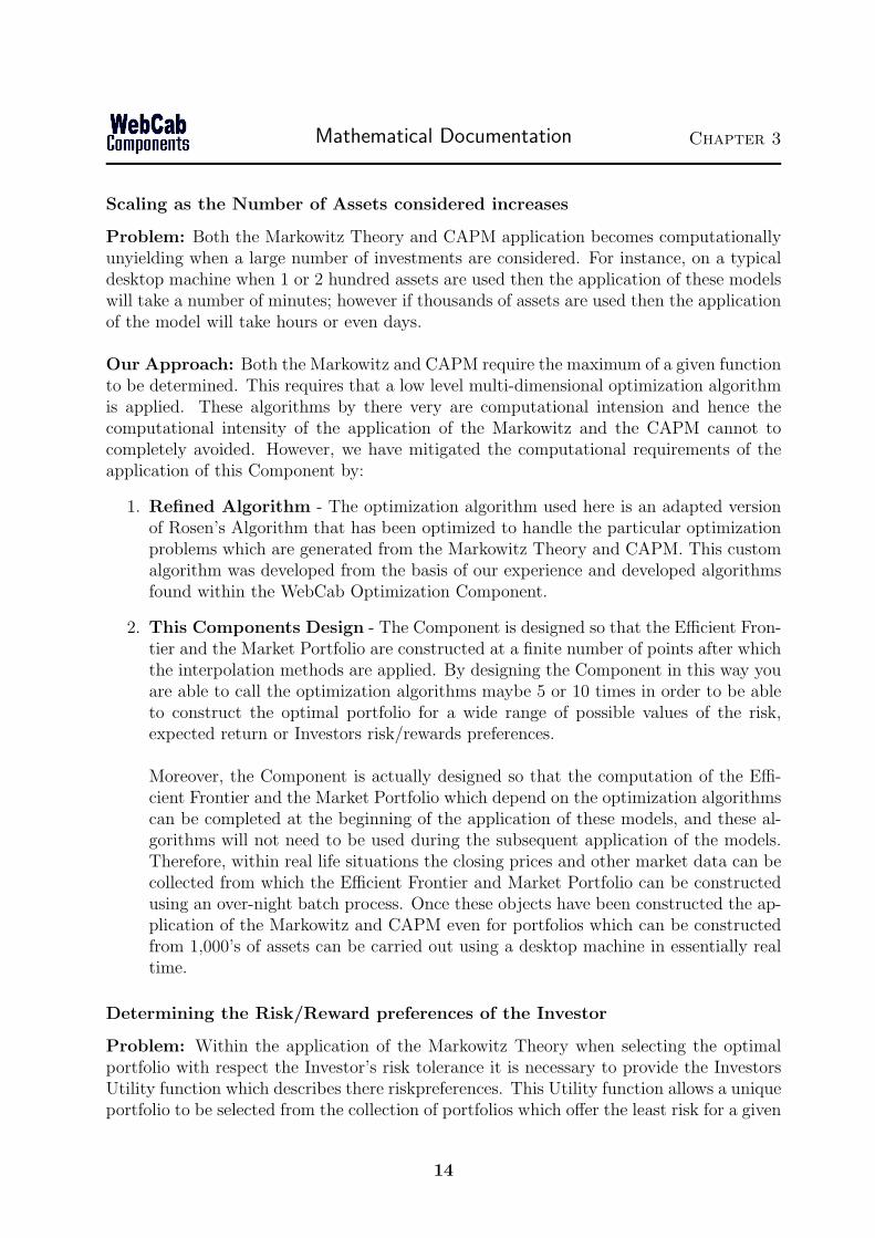
Scaling as the Number of Assets considered increases
Problem: Both the Markowitz Theory and CAPM application becomes computationallyunyielding when a large number of investments are considered. For instance, on a typicaldesktop machine when 1 or 2 hundred assets are used then the application of these modelswill take a number of minutes; however if thousands of assets are used then the applicationof the model will take hours or even days.
Our Approach: Both the Markowitz and CAPM require the maximum of a given functionto be determined. This requires that a low level multi-dimensional optimization algorithmis applied. These algorithms by there very are computational intension and hence thecomputational intensity of the application of the Markowitz and the CAPM cannot tocompletely avoided. However, we have mitigated the computational requirements of theapplication of this Component by:
1. Refined Algorithm - The optimization algorithm used here is an adapted versionof Rosen’s Algorithm that has been optimized to handle the particular optimizationproblems which are generated from the Markowitz Theory and CAPM. This customalgorithm was developed from the basis of our experience and developed algorithmsfound within the WebCab Optimization Component.
2. This Components Design - The Component is designed so that the Efficient Fron-tier and the Market Portfolio are constructed at a finite number of points after whichthe interpolation methods are applied. By designing the Component in this way youare able to call the optimization algorithms maybe 5 or 10 times in order to be ableto construct the optimal portfolio for a wide range of possible values of the risk,expected return or Investors risk/rewards preferences.
Moreover, the Component is actually designed so that the computation of the Effi-cient Frontier and the Market Portfolio which depend on the optimization algorithmscan be completed at the beginning of the application of these models, and these al-gorithms will not need to be used during the subsequent application of the models.Therefore, within real life situations the closing prices and other market data can becollected from which the Efficient Frontier and Market Portfolio can be constructedusing an over-night batch process. Once these objects have been constructed the ap-plication of the Markowitz and CAPM even for portfolios which can be constructedfrom 1,000’s of assets can be carried out using a desktop machine in essentially realtime.
Determining the Risk/Reward preferences of the Investor
Problem: Within the application of the Markowitz Theory when selecting the optimalportfolio with respect the Investor’s risk tolerance it is necessary to provide the InvestorsUtility function which describes there riskpreferences. This Utility function allows a uniqueportfolio to be selected from the collection of portfolios which offer the least risk for a given
14

Mathematical Documentation Chapter 3
expected return. The difficulty here like with other non-observable quantities is in our abil-ity to estimate this function from information which is provided by the investor.
Our Approach: The difficulty in obtaining the Investors Utility Function is in providinga framework which is both comprehensive and user friendly. Ideally, the Investors wouldbe in a position to submit a function (in analytic form or otherwise) which relates the riskand expected return in accordance with his preferences. However, this requirement and re-sulting construction of the Utility function if not sufficiently intuitive in order to be widelyapplied. The approach we have taken here is to allow the Investor to given his risk/rewardpreferences at a finite number of sweet stops around which we will interpolate in order toobtain the Utility function itself. Clearly, one of the assumptions we are forced to makein this approach is that the Utility function is smoothly varying between the interpolationpoints given.
Remark The interval between and the location of the interpolation points should re-flect nature of the investors preferences. In particular, in regions where the cubic splineinterpolation function is likely to differ most from the (true) Utility function more inter-polation points should be requested from the investor.
For further details concerning the application of this (and other) approaches please seethe section ‘Discovering the Investors risk - return profile’).
Practicalities of Diversification
Problem: Though this problem is not particular to our (or others) implementations itis important to point out that in practice costs will be incurred when an asset is broughtor sold, and the effects of diversification (in accordance with the Markowitz Theory andCAPM) will diminish as the number of assets considered within the collection of assetincreases. Therefore in practice one should balance the benefits of diversification with thecosts incurred in re-balancing a portfolio.
Solution: The level of costs will vary according to the type and quantity of assets beingheld within the portfolio. Generally speaking the more liquid the asset the lower the rel-ative transaction costs will be for a given transaction size. Moreover, several studies haveshown that it is possible to derive most of the benefits of diversification with a portfolioconsisting of 12 to 18 holdings. That is, to be adequately diversified does not require 200holdings in a portfolio which could incur significant trading costs.
Another approach to deducing the effects of trading costs is to use derivatives on the un-derlying assets rather than the assets themselves in order to rebalance the portfolios. Thereason being that derivatives trading generally has significantly lower costs than tradingin the underlying security.
15

Mathematical Documentation Chapter 3
3.2 Preliminaries and Auxiliary class’s
Within this section we details a number of auxiliary notions and the procedures with willbe required by the main functionality offered by this Component.
Within the :Portfolio:AssetParameters: class we provide procedures for the evaluationof various quantities which are required within the application of this Component. Theseparameters include:
• Estimate of the Volatility of an asset prices:
1. Historical Approach: :Portfolio:AssetParameters:volatility(double[]):
2. Scenario Approach: :Portfolio:AssetParameters:volatility(double[], double[]):
• Estimate Expected Return of an asset:
1. Historical Approach: :Portfolio:AssetParameters:expectedReturn(double[]):
2. Scenario Approach: :Portfolio:AssetParameters:expectedReturn(double[], dou-ble[]):
3. ARCH based Approach: :Portfolio:AssetParameters:archExpectedPriceEstimate:
• Estimate Covariance Matrix of the collection assets:
1. Historical Approach: :Portfolio:AssetParameters:covarianceMatrix(double[][]):
2. Scenario Approach: :Portfolio:AssetParameters:covarianceMatrix(double[],double[][]):
Note Further methods for the estimation of the Volatility are provided within the :Port-folio:Volatility: class.
3.2.1 Choices in Approach and other issues
As listed about the main two approaches by which the expected return, volatility andcovariance are estimates is the historical and scenarios based approaches. Here we motivatethe essential differences between these methods. We also give a brief explanation of theARCH procedure for the estimation of the expected returns along with advice concerningthe number of historical values which should be used within the application of the historicalestimate.
When should the scenario approach be used?
One such instance is when a takeover of a quoted company has been announced andthe share price converges to almost the offer price in anticipation of the takeover beingcompleted. In this scenario the more likely the takeover will be completed the closer theprice will converge to the offer price. However, if the takeover breaks down then the priceis likely to experience sharp moves to the price level found prior to the intended takeoverbeing announced. By estimating the likely-hood of each scenario and the likely level ofvolatility resulting we are able to give a realistic forward looking estimate.
16

Mathematical Documentation Chapter 3
When should the historical approach be used?
If the market under consideration goes through seasonal or business cycles, or if a givencompany has transformed itself then the observations used in order to estimate the expectedvolatility should reflect these issues. For example, if company which was a diversifiedgeneral industrial company has since refocused on certain key areas, then in terms ofestimating its expected volatility from historical values it is reasonable to only considerthe period after the company refocused.
The number of historical values which should be used
The number of historical values used here in order to estimate the volatility should reflectthe length of the period over which a reliable estimate of the volatility is required. Forexample, if an estimate of the 1-month volatility is sort then it is reasonable to use at leastthe last 1-months historical values up to a few years of historical values.
ARCH type models for Estimate Returns and Volatility
The ARCH model in the general sense can be thought of as a (linear) weighted scheme.Here we allow the past historical asset prices to have a weighted effect, along with aweighted measurement of the expected value in accordance with the assets characteristicline. Note, that when we set all the weights of the historical values to zero this estimatereduces to an estimate based on extrapolation of the characteristic line.
When to use the ARCH approach
This method assumes that the asset under consideration exhibits a long term drift (inparticular, linear correlation) with respect to some market index. Therefore, this estimateis particularly applicable to assets which have been observed to exhibit significant linearlycorrelation to market indexes such as the FT100, S&P500 etc.
3.2.2 Basic Formulae for the Return, Covariance, Correlationand Risk
Within this subsection we collect together a number of formulae which illustrate how thescenario and the historical approach can be used in order to either define or investigaterelationships between the return, covariance, correlation or risk of a portfolio and its assets.
Definition of the Return of a Portfolio
Before we move onto the Markowitz Theory we should define exactly what we mean by thereturn of a portfolio. The return of a portfolio over a given period is simply the weightedarithmetic average of the returns of the individual assets. That is, the return rp of a
17
Mathematical Documentation Chapter 3
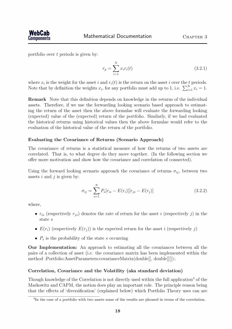
portfolio over t periods is given by:
rp =N∑
i=1
xiri(t) (3.2.1)
where xi is the weight for the asset i and ri(t) is the return on the asset i over the t periods.Note that by definition the weights xi, for any portfolio must add up to 1, i.e.
∑Ni=1 xi = 1.
Remark Note that this definition depends on knowledge in the returns of the individualassets. Therefore, if we use the forwarding looking scenario based approach to estimat-ing the return of the asset then the above formulae will evaluate the forwarding looking(expected) value of the (expected) return of the portfolio. Similarly, if we had evaluatedthe historical returns using historical values then the above formulae would refer to theevaluation of the historical value of the return of the portfolio.
Evaluating the Covariance of Returns (Scenario Approach)
The covariance of returns is a statistical measure of how the returns of two assets arecorrelated. That is, to what degree do they move together. (In the following section weoffer more motivation and show how the covariance and correlation of connected).
Using the forward looking scenario approach the covariance of returns σij, between twoassets i and j is given by:
σij =N∑
s=1
Ps[ris − E(ri)][rjs − E(rj)] (3.2.2)
where,
• ris (respectively rjs) denotes the rate of return for the asset i (respectively j) in thestate s
• E(ri) (respectively E(rj)) is the expected return for the asset i (respectively j)
• Ps is the probability of the state s occurring
Our Implementation: An approach to estimating all the covariances between all thepairs of a collection of asset (i.e. the covariance matrix has been implemented within themethod :Portfolio:AssetParameters:covarianceMatrix(double[], double[][]):.
Correlation, Covariance and the Volatility (aka standard deviation)
Though knowledge of the Correlation is not directly used within the full application4 of theMarkowitz and CAPM, the notion does play an important role. The principle reason beingthat the effects of ‘diversification’ (explained below) which Portfolio Theory uses can are
4In the case of a portfolio with two assets some of the results are phrased in terms of the correlation.
18
Mathematical Documentation Chapter 3
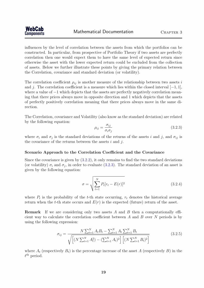
influences by the level of correlation between the assets from which the portfolios can beconstructed. In particular, from prospective of Portfolio Theory if two assets are perfectlycorrelation then one would expect them to have the same level of expected return sinceotherwise the asset with the lower expected return could be excluded from the collectionof assets. Below we further illustrate these points by giving the primary relation betweenthe Correlation, covariance and standard deviation (or volatility).
The correlation coefficient ρij is another measure of the relationship between two assets iand j. The correlation coefficient is a measure which lies within the closed interval [−1, 1],where a value of −1 which depicts that the assets are perfectly negatively correlation mean-ing that there prices always move in opposite direction and 1 which depicts that the assetsof perfectly positively correlation meaning that there prices always move in the same di-rection.
The Correlation, covariance and Volatility (also know as the standard deviation) are relatedby the following equation:
ρij =σij
σiσj
(3.2.3)
where σi and σj is the standard deviations of the returns of the assets i and j, and σij isthe covariance of the returns between the assets i and j.
Scenario Approach to the Correlation Coefficient and the Covariance
Since the covariance is given by (3.2.2), it only remains to find the two standard deviations(or volatility) σi and σj, in order to evaluate (3.2.3). The standard deviation of an asset isgiven by the following equation:
σ =
√√√√ N∑t=1
Pt[rt − E(r)]2 (3.2.4)
where Pt is the probability of the t-th state occurring, rt denotes the historical averagereturn when the t-th state occurs and E(r) is the expected (future) return of the asset.
Remark If we are considering only two assets A and B then a computationally effi-cient way to calculate the correlation coefficient between A and B over N periods is byusing the following expression:
σij =N
∑Nt=1 AtBt −
∑Nt=1 At
∑Nt=1 Bt√[
(N∑N
t=1 A2t )− (
∑Nt=1 At)2
] [(N
∑Nt=1 Bt)2
] (3.2.5)
where At (respectively Bt) is the percentage increase of the asset A (respectively B) in thetth period.
19

Mathematical Documentation Chapter 3
Evaluating the Expected Return(s) (Scenario Approach)
The following expression is often used to define (average) expected return E(r) of an assetover some (future) time period:
E(r) =N∑
s=1
Psrs (3.2.6)
where Ps is the probability of the state s occurring and rs is the corresponding expectedreturn of that given state.
Our Implementation: Such an approach has been implemented within :AssetParam-eters:expectedReturn)double[], double[]):.
Covariance of the Expected Return (Historical Approach)
Similarly, we may use an historical approach in order to estimate the covariance betweenthe expected return of assets. That is, if we know the historical rates of return then thecovariance is given by the expression:
σij =1
N
N∑t=1
(rit − ri)(rjt − rj) (3.2.7)
where,
• N is the number of equally likely paired observations
• rit (respectively rjt) is the return of the asset i (respectively j) in the tth period
• ri (respectively rj) is the historical average return for the asset i (respectively j)
Our Implementation: The allow the covariance to be evaluated/estimated uses a sce-nario or historical approach within :Portfolio:AssetParameters:covariance(double[],double[],double[]):, or :Portfolio:AssetParameters:covariance(double[],double[]): respectively. Theevaluation of the covariance is only required when portfolio with only two assets are re-quired. For portfolio with more than two assets you will be required to evaluate the covari-ance matrix of the collection of assets from which the portfolio can be constructed. Withinthe :Portfolio:AssetParameters: class we provide the methods :Portfolio:AssetParameters:covarianceMatrix(double[][]):,and :Portfolio:AssetParameters:covariance(double[],double[][]):, which allow the covariancematrix to be evaluated via historical or a scenario based approach respectively.
Variance and Expected Return of a Portfolio with n holdings
We give the general formula for the variance σ2(rp), of the returns for a portfolio of Nassets:
var(rp) = σ2(rp) =N∑
i=1
x2i σii +
N∑i=1
N∑j=1
xixjσij for i = j (3.2.8)
20
Mathematical Documentation Chapter 3
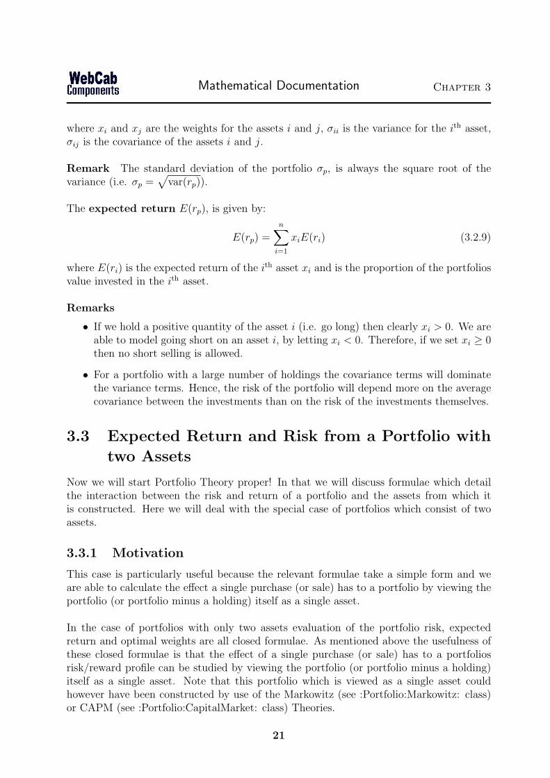
where xi and xj are the weights for the assets i and j, σii is the variance for the ith asset,σij is the covariance of the assets i and j.
Remark The standard deviation of the portfolio σp, is always the square root of thevariance (i.e. σp =
√var(rp)).
The expected return E(rp), is given by:
E(rp) =n∑
i=1
xiE(ri) (3.2.9)
where E(ri) is the expected return of the ith asset xi and is the proportion of the portfoliosvalue invested in the ith asset.
Remarks
• If we hold a positive quantity of the asset i (i.e. go long) then clearly xi > 0. We areable to model going short on an asset i, by letting xi < 0. Therefore, if we set xi ≥ 0then no short selling is allowed.
• For a portfolio with a large number of holdings the covariance terms will dominatethe variance terms. Hence, the risk of the portfolio will depend more on the averagecovariance between the investments than on the risk of the investments themselves.
3.3 Expected Return and Risk from a Portfolio with
two Assets
Now we will start Portfolio Theory proper! In that we will discuss formulae which detailthe interaction between the risk and return of a portfolio and the assets from which itis constructed. Here we will deal with the special case of portfolios which consist of twoassets.
3.3.1 Motivation
This case is particularly useful because the relevant formulae take a simple form and weare able to calculate the effect a single purchase (or sale) has to a portfolio by viewing theportfolio (or portfolio minus a holding) itself as a single asset.
In the case of portfolios with only two assets evaluation of the portfolio risk, expectedreturn and optimal weights are all closed formulae. As mentioned above the usefulness ofthese closed formulae is that the effect of a single purchase (or sale) has to a portfoliosrisk/reward profile can be studied by viewing the portfolio (or portfolio minus a holding)itself as a single asset. Note that this portfolio which is viewed as a single asset couldhowever have been constructed by use of the Markowitz (see :Portfolio:Markowitz: class)or CAPM (see :Portfolio:CapitalMarket: class) Theories.
21

Mathematical Documentation Chapter 3
3.3.2 Formulation for a Portfolio of two assets
If we can construct portfolios from two assets A and B, then the general portfolio P ,will take the form:
P = αE(RA) + (1− α)E(RB)
where {α : 0 ≤ α ≤ 1}, determines the weighting of the portfolio between the two assetsA and B.
If the corresponding expected returns of the two asset from which portfolio can beconstruct are E(RA) and E(RB), then the expected return of the general portfolio E(Rp)is:
E(Rp) = αE(RA) + (1− α)E(RB) (3.3.10)
with a standard deviation of:
σp =√
α2σ2A + (1− α)2σ2
B + 2α(1− α)σAB (3.3.11)
By using the identity (3.2.3), σAB = σAσBρAB, we can rewrite (3.3.11) as:
σ2p = α2σ2
A + (1− α)2σ2B + 2α(1− α)σAσBρAB (3.3.12)
3.3.3 Minimum risk of a portfolio with two assets
By direct calculation for a two-asset portfolio composed of the assets A and B, the portfoliowith the minimum risk for some corresponding value of the expected return occurs whenthe weighting of the asset A (α) is equal to:
α =σ2
B − ρABσAσB
σ2A + σ2
B − 2ρABσAσB
where α is the percentage (in decimal format) invested in asset A within the two assetportfolio. Hence the percentage invested in the other asset B is (1− α).
In particular, for the special cases when the assets are uncorrelated (i.e. knowledge ofthe movement of one asset either up or down does not imply anything concerning themovement of the other) and perfectly negatively correlated (i.e. the assets always move ofopposite directions)we have:
• A and B are uncorrelated (i.e. σAB = 0) is given by:
α =σ2
B
σ2A + σ2
B
(3.3.13)
• A and B are perfectly negatively correlated (i.e. σAB = −1) is given when:
α =σB
σA + σB
(3.3.14)
22
Mathematical Documentation Chapter 3
Concluding Remarks: Above we have constructed the portfolio under various conditionswhich exhibits the minimal risk which some expected return. However, often an investorwill wish to balance the risk against the return which is the main question we will considerthe following sections.
3.4 Markowitz Theory
The Markowitz Model is used to analyze the construction and qualitative nature of a port-folio’s risk-return characteristics. In particular, we offer methods by which the continuum(in risk and expected return) of the portfolios (known as the Efficient Frontier) whichconsists of the portfolios with the minimum risk for a given value of the expected returnconstructed from a given collection of assets. Moreover, from this collection of Portfoliosa unique optimal portfolio can be selected with respect to a given value of the expectedreturn, risk or an investors risk - return profile given in terms of a utility function.
3.4.1 Overview of Markowitz Theory Implemented
The Efficient Frontier is the collection of portfolios constructed from the given set of assetswhich have the lowest possible risk for a given level of the expected return. Note that theweights of the assets making up the portfolio may themselves be subject to constraints (forexample, no one asset can have a weighting more than 20 percent or less the 5 percent)which we will deal with below.
Once the Efficient Frontier is known, we are able to select from this continuum a uniqueportfolio which represent the optimal portfolio with respect to an investors risk - returnprofile. The return profile of the investor may be given in three distinct ways and thecorrespond optimal portfolio can them be constructed. The by one of the following means:
1. With respect to the investors risk - reward utility function, see :Portfolio:Markowitz:setUtilityFunctionInterp,:Portfolio:Markowitz:setUtilityFunctionPoly:.
2. Maximum Risk - the investor gives the (maximum) risk which they are prepared toaccept and then the corresponding portfolio with the highest expected return for thatgiven level of risk is constructed.
3. Expected Return - the investor gives the expected return which they desire and theportfolio with the least risk for that given level of expected return is constructed.
3.4.2 Construction of the Efficient Frontier
For a given collection of securities with various risk profiles, an investor can construct awhole range of portfolios with various risk-return characteristics. In particular, there ex-ists a continuous family of portfolios within the range of the risk and expectation of theindividual securities. The investor will wish to choose a portfolio from this family whichoffers the lowest level of risk for a given expected return, according to the assumptions of
23

Mathematical Documentation Chapter 3
the Markowitz model.
We consider the family of all possible portfolios formed from a combination of the availablesecurities. Within this family we choose a locus of points by selecting the portfolios whichoffer the least risk for a given level of the expected return. Such optimal portfolios willexist within the range of the expected returns. This locus of points is referred to as theEfficient Frontier.
The Efficient Frontier is constructed by the following steps:
1. Evaluated the Efficient Frontier at a finite number of points. That is find the portfoliowhich exhibit the lowest risk for a given expected return.
2. Interpolate about these points using cubic spline (or some other method) in order toconstruct the Efficient Frontier.
The points on the Efficient Frontier are portfolios constructed from the set of assets con-sidered which exhibit the lowest risk for a given expected return. These portfolio arecharacterized by the following three characteristics:
1. Expected Return - The expected return of the portfolio which is estimated from thehistorical returns of the assets within the portfolio.
2. Total Risk - The total risk of the portfolio which is estimated from the historicalreturns of the assets within the portfolio.
3. Asset Weights - the weights of the collection of assets from which the portfolio canbe constructed.
It is important to point out that the Efficient Frontier in monotonically increasing functionin risk and expected return. This means that if we are given a value of the expected returnthen there will correspond a unique portfolio on the Efficient Frontier with a given totalrisk. Conversely, if we are given the total risk of the portfolio then there will exist a uniqueportfolio on the Efficient Frontier with a corresponding value its expected return.
Constraining the Weights of the assets of the Efficient Frontier’s Portfolios
Within our implementation we offer the possibility to constrain the weights of the assetsfrom which the portfolios on the Efficient Frontier are constructed. The constraints on theweights on the portfolios are set by using the method setConstraints. We illustrate the useconstraints with the following example.
Say an investor requires a portfolio selected from n asset which has the lowest risk fora given expected return but also has the requirement that all of the assets must have aweight between 0.05 and 0.1 (i.e. between 5 and 10 percent). In this instance we wouldneed to set the constraints on the assets to be:
24

Mathematical Documentation Chapter 3
lowerBounds = { 0.05, 0.05, 0.05,...., 0.05 }upperBounds = { 0.1, 0.1, 0.1, ......, 0.1 }
where each of the arrays above has the same number of terms as the number of assetsfrom which the portfolio can be constructed. Constraints can be set on the assets fromwhich the Efficient Frontier is constructed by using :Portfolio:Markowitz:setConstraints:,constraints can also be added within the context of the evaluation of the Efficient Frontierwithin the CAPM using :Portfolio:Markowitz:setConstraints:.
Remark: If the constraints are not set then they will take there default values whichare 0 and 1, for the lower bound respectively upper bound of each asset. That is, they willremain as weights in the usual sense.
3.4.3 Constraints effect on the range of the Efficient Frontier
The placing of constraints on the weights of the assets effects the range of expected returnsfor which the resulting portfolios can be constructed. Since the (constrained) EfficientFrontier is just a collection of portfolios subject also subject to the constraints which min-imize the risk for a given level of the expected return. The range of values over which theEfficient Frontier exists must correspond to the range of expected returns of the possibleconstructed portfolios.
Within the Markowitz and the CapitalMarket class’s we provide the methods maxFrontierReturn,and minFrontierReturn we allow the maximum and respectively minimum values of theexpected return over which the (possibly constrained) Efficient Frontier exists. We alsooffer two associated methods maxFrontierReturnWeights and minFrontierReturnWeights,which evaluate the assets weights of the portfolio at these two ends points. These twomethods which construct the Portfolios on the Efficient Frontier at its end points have thesignificant advantage of having almost no computational overhead, unlike the constructionof the portfolios on the Efficient Frontier at other points.
Also, note that since the Efficient Frontier is monotonically increase in risk and expectedreturn, the therefore the point at which the maximum and minimum expected return onthe Efficient Frontier occur is also the points at which the maximum respectively minimumof the risk of the portfolios on the Efficient Frontier occur.
Performance Issues
The introduction of constraints on the weights of the portfolios which form the EfficientFrontier will have the following consequences with regards to overall performance:
• Upper Bounds - the presence of upper bounds (not all equal to 1) on the assetweights will result in the construction of the corresponding Efficient Frontier requiringsignificantly more computational resources. If however the upper bounds are all setto 1 (i.e. there default value), then they will not effect the computational demands
25
Mathematical Documentation Chapter 3
required to evaluate the points on the Efficient Frontier. This allows lower boundsto be set on the asset weight without reducing the performance of this class.
• Lower Bounds - the presence of lower bounds on the asset weights will have nosignificant effects on the efficiency of the construction and analysis of portfolio onthe Efficient Frontier.
Notes on the Evaluation of the Efficient Frontier and the Optimal Portfolio
To calculate the Efficient Frontier, Rosen’s gradient projection optimization algorithm isused. If you directly try to evaluate the optimal portfolio with respect to an investorsutility function then you will need numerous applications of Rosen’s algorithm which willbecome computationally intensive. Therefore, we designed this class so that this wouldnot be necessary by allowing the computation at the beginning a number of points onthe Efficient Frontier, from which the other points will be deduced (in fact, estimated)through the use of cubic spline interpolation. These interpolation points are determinedby calculateEfficientFrontier, which must be called prior to any subsequent method whichdepends on the Efficient Frontier being known.
The use of this approach will also allow us to deal with the possible situation.
3.4.4 Consistency of the Assets and Effects on the Efficient Fron-tier
This section deals with a rather technical issue concerning how the consistency of the col-lection of assets from which the Portfolio on the Efficient Frontier can be constructed. Byconsistency we mean consistency with the assumptions of Markowitz Theory and CAPM,and how these inconsistencies effect are ability the construct optimal portfolio in a neigh-borhood of the lower bound of the expected returns over which the Efficient Frontier exists.That is, how appropriate the portfolios constructed from the available (“inconsistent”) as-sets are to issues concerning the selection of the optimal portfolio. Hence the selectionof either portfolios with the lowest risk for a given expected return or portfolio with thehighest expected return with a given maximum risk.
When these effects occur
Note that the effects we will consider with this section will have relevance in the followingsituations:
• Only effect a neighborhood of the lower bound of the expected returns over whichthe Efficient Frontier exists.
• Will only occur when the portfolio considered are constructed from collections ofassets which are not consistent (see note below) the assumptions of Markowitz Theoryand CAPM.
26
Mathematical Documentation Chapter 3
Remark Similar effects do not occur in a neighborhood of the upper bound of the ex-pected return of the Efficient Frontier because at the upper bound by definition there donot exist any portfolios with a higher expected returns so for that level of returns thereare no preferred portfolios.
Advice to the Reader
We advise the reader to skip this section at the first reading, and refer back if you en-counter such effects with the collection of assets you are using in order to construct theportfolios within your given application.
Nature of Inconsistency
The way in which the collection of assets can be inconsistent lies in the fact that theMarkowitz Theory (and as we will see later the CAPM) assume that the investor will onlytake on additional risk for a higher level of expected return. Therefore, in order for acollection of assets to be consistent with these assumptions there must exist a portfoliowith a greater return if it has a higher risk. Unfortunately, this may not be the case if theassets do not obey the rule that for a higher level of the expected return the risk increases.
If such a portfolio exists then the Efficient Frontier should only be considered on a subsetover the entire range of expected values on which it exists when selecting an optimal port-folio. In particular, we will need to increase the lower bound of the expected returns overwhich the Efficient Frontier is considered. The precise construction of the lower bound willin general involve analysis of the differential of the Efficient Frontier. We implement theseprocedures within the MaxRange class.
When Inconsistency will effect the Efficient Frontier application
He we detail when the effects of inconsistency of the historical source data will effectthe Efficient Frontiers ability the select the optimal portfolio. We only offer conditionsunder which such effects are certain to take place. We refer the reader to the section onprecise lower bounds for a precise statement under which this effect take place take place.
When the asset with the lowest expected return does not have an upper bound on itsweight then this effect is certain to occur when:
‘the asset with the lowest expected return does not have the lowest risk anddoes not have a constraint placed on its upper bound’
In the case when this asset does not have an upper bound on its asset weight then theseeffects are certain to take place if:
‘The portfolio constructed by taking the maximum weight of the asset with thelowest expected return, then the maximum weight of the asset with the next
27
Mathematical Documentation Chapter 3
to lowest expected return and so on... until the sum of the weights is one. Ifthere exists an asset from the remaining assets with a higher expected returnwith a lower risk.’
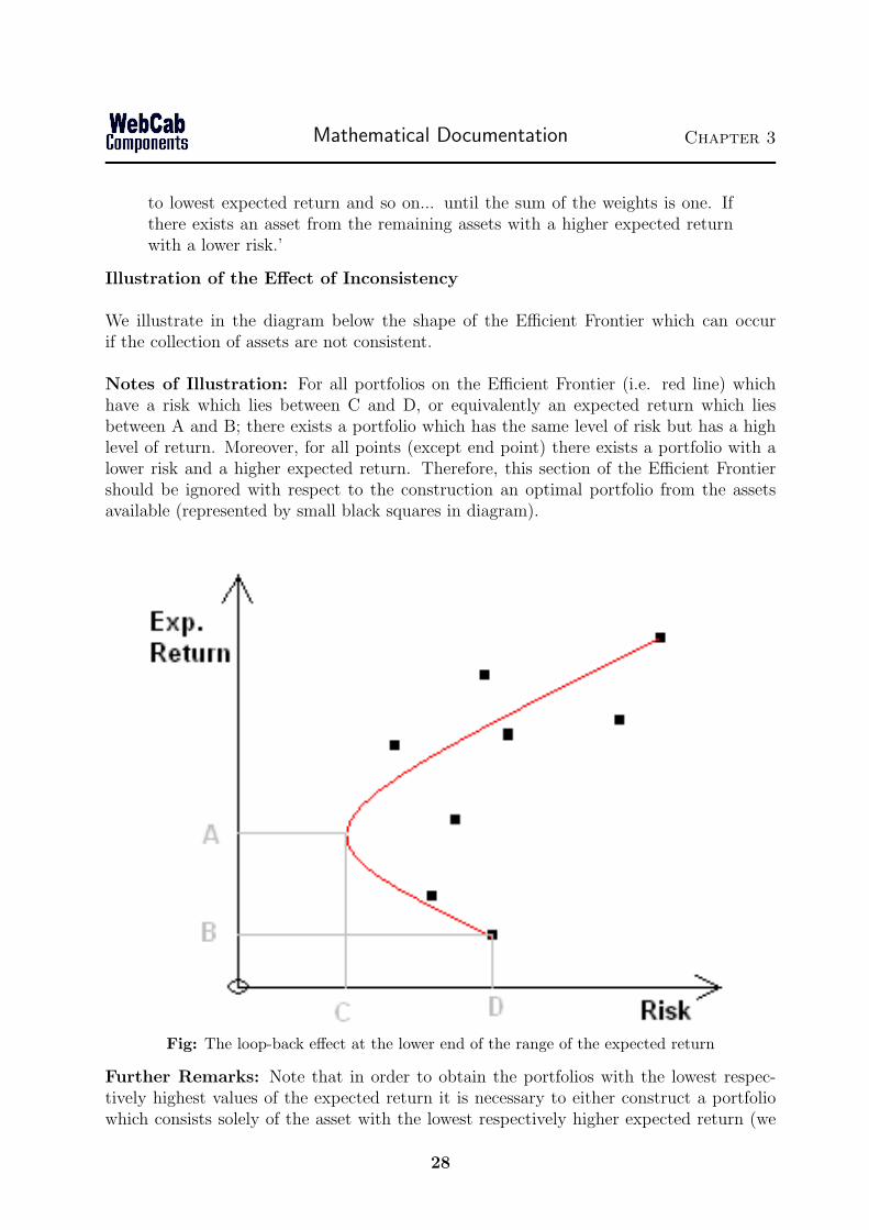
Illustration of the Effect of Inconsistency
We illustrate in the diagram below the shape of the Efficient Frontier which can occurif the collection of assets are not consistent.
Notes of Illustration: For all portfolios on the Efficient Frontier (i.e. red line) whichhave a risk which lies between C and D, or equivalently an expected return which liesbetween A and B; there exists a portfolio which has the same level of risk but has a highlevel of return. Moreover, for all points (except end point) there exists a portfolio with alower risk and a higher expected return. Therefore, this section of the Efficient Frontiershould be ignored with respect to the construction an optimal portfolio from the assetsavailable (represented by small black squares in diagram).
Fig: The loop-back effect at the lower end of the range of the expected return
Further Remarks: Note that in order to obtain the portfolios with the lowest respec-tively highest values of the expected return it is necessary to either construct a portfoliowhich consists solely of the asset with the lowest respectively higher expected return (we
28

Mathematical Documentation Chapter 3
assume that these assets weights are not constrained). For this reason there is a rationalefor considering the Efficient Frontier at both of these points, since they are unique theymust by definition be the portfolio with that given (exact) level of return with the lowestrisk. However from the prospective of selecting the optimal portfolio corresponding to anexpected return at A (in the above diagram), it is not appropriate.
Another motivation for including the portfolio corresponding the A, and similar non-optimalportfolios in the Efficient Frontier is that the portfolios at the extremes of the Efficient Fron-tier lie at the vertex of the arced region (see dark gray shading in diagram below) in whichall the possible portfolios which can be constructed from the available assets lie.
Fig: All possible portfolios lie within the dark gray region.
Approximate Lower Bound of the ‘Maximum Range’
Therefore, from the point of view of applying the Efficient Frontier to selecting the optimalportfolio we will need to evaluate a (new) lower bound greater than the bound over whichthe Efficient Frontier exists over which the Frontier does only contain (justifiable) optimalportfolios. Here we will provide a quick and easy approach which allows a lower bound tobe evaluated. Note that this lower bound will often not be optimal.
No Upper Bound Constraint on asset with the Lowest Risk
29

Mathematical Documentation Chapter 3
In the case when there are no constraints placed on the weight of the asset with the lowestrisk we are able to evaluate the (approx.) range of the expected return which should beused when constructing the optimal portfolio is given by:
• Upper Bound on the Expected Returns: The expected return of the asset with thehighest expected return.
• Lower Bound on the Expected Returns: The expected return of the asset with thelowest RISK.
If you use this range of expected returns then the Efficient Frontier constructed will notdisplay the problem of suggesting the below optimal portfolio. Note that in this instance ifyou require a portfolio below this lower bound of the expected return for which the existsan portfolio (i.e. an expected return is above the expected return of the asset with thelowest expected return and below the lower bound set). Then you should just select theportfolio on the Efficient Frontier with a risk equal to the risk of the asset with the lowestrisk.
With Constraints
In the case when there are constraints on the weights of the assets (or at least an upperbound constraint on the asset with the lowest risk) then a construction based on similarprinciples applies. This construction is as follows:
• Upper Bound on the Expected Returns: The expected return of the asset with thehighest expected return.
• Lower Bound on the Expected Returns: If you have an upper bound on the assetwith the lowest risk then form a portfolio by taking the maximum weight of this assetthen the asset with the next highest risk and so on... until the sum of the weights isone. Then the lower bound on the expected return should be the expected return ofthe portfolio constructed in this means.
These constructions have been implemented and offered as public methods within theMaxRange class.
Discussion and Illustration of this Approach
In the below diagram we illustrate this approach. Note that in this case the lower boundcorresponding to a risk of F, is not optimal since the optimal points has an expected returnof A, and risk of C. Also, note that only the Efficient Frontier to the right of the intersectionwill be considered (denoted by the arrow).
30
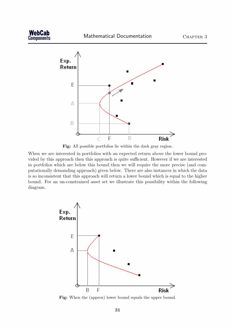
Mathematical Documentation Chapter 3
Fig: All possible portfolios lie within the dark gray region.
When we are interested in portfolios with an expected return above the lower bound pro-vided by this approach then this approach is quite sufficient. However if we are interestedin portfolios which are below this bound then we will require the more precise (and com-putationally demanding approach) given below. There are also instances in which the datais so inconsistent that this approach will return a lower bound which is equal to the higherbound. For an un-constrained asset set we illustrate this possibility within the followingdiagram.
Fig: When the (approx) lower bound equals the upper bound.
31
Mathematical Documentation Chapter 3
Exact Evaluation of the Lower Bound of the ‘Maximum Range’
Though the above approach will yield an range over which all portfolios of the EfficientFrontier are optimal portfolios, the lower bound on the range of expected returns will notin general be optimal. In order to provide a precise evaluation of the lower bound of theexpected return we will need to use an algorithm which considers the differential of theEfficient Frontier. In particular, we will need to construct the Efficient Frontier of thepossibly constrained assets and evaluate unique point (if it exist) where the rate of changeof the risk with respec to the expected return is zero. If this point is a minimum thenthe corresponding value of the expected return at that point is the precise lower boundover which the Efficient Frontier should be considered when used to construct an optimalportfolio.
We use this indirect (i.e. via Frontier) approach because even if the historical source datais not consistent with the assumptions of Portfolio Theory the above mentioned effects maynot take effect. We offer procedures which deal with this case within the MaxRange class.
3.4.5 Selecting the Optimal Portfolio
The construction of a portfolio with regard to an investors risk - reward profile lies at thecore of Markowitz Theory. By obtaining information concerning the value judgments tothe various risk - reward combinations which will be available to the investor we are able toselect the optimal (or preferred) portfolio for the continuum of portfolios on the EfficientFrontier. If we where not aware of a given investors risk preferences then it would not bepossible to select a preferred portfolio on the Efficient Frontier. There are different levelof granularity of the investors preferences which are sufficient in order to select an optimalportfolio. At one end the investor may only provide information concerning the maximallevel of risk acceptable or the level of expected return desired from which an optimal port-folio can be selected. On the other hand the investors utility function may be given whichoffers much more fine grained information concerning this investors risk-reward preferencesand allows a value judgment to be assign to a continuum of risk-reward combinations.
As mentioned above and within the over view of this section within Markowitz Theorythere are essentially three ways in which to select an optimal portfolio from the selectionof portfolios known as the Efficient Frontier which are each optimal for there correspond-ing value of the expected return or risk. The three mechanism for selection the optimalportfolio are as follows:
1. Give value of the Expected Return - Since the Efficient Frontier is monotonicallyincreasing and continuous in the expected return a point and hence portfolio can beselected for a given value of the expected return over the range of the expected return.Once the (possibly constrained) Efficient Frontier has been constructed we are able toselect an optimal portfolio by using :Portfolio:Markowitz:efficientFrontier(double,int):;alternatively you may wish to use the approach of :Portfolio:Markowitz:findRisk(double,double[], double[]):
32

Mathematical Documentation Chapter 3
2. Given value of the Risk - Since the Efficient Frontier is monotonically increasingand continuous in the value of the risk a point and hence portfolio can be selectedfor a given value of the expected return over the range of the total risk. Once the(possibly constrained) Efficient Frontier is known we are able to select an optimalportfolio by using :Portfolio:SolveFrontier:findReturn(double, double[], double[]):
3. Provide the Investors Utility Function - The investors utility function is thelocus of points at which the investor gets a particular level of satisfaction or utilityfrom a combination of expected return and risk. This function may be a functionwith respect to the expected return or risk. By identifying the points at which theutility function and Efficient Frontier coincide we are able to identify a collection ofportfolios which are optimal with respect to the investors expressed risk/return pref-erences. If the utility function is given as a function of the expected return then youcan use :Portfolio:Markowitz:optimalPortfolio(double, double, double[][]):, :Portfo-lio:Markowitz:optimalPortfolioMaxExpected(double, double, double[][]):, or alterna-tively you may wish to use the approach; :Portfolio:SolveFrontier:findRisk(double[],double[], double[], double[], double):. If the utility function is given as a function ofthe total risk then the you will need to used :Portfolio:SolveFrontier:findReturn(double[],double[], double[], double[], double):. For further details concerning the details of ourimplementation we refer the reader to :Portfolio:Markowitz: or :Portfolio:CapitalMarket:
Since the Efficient Frontier is monotonically increasing in the expected return and riskthe application and nature of selecting the optimal portfolio from knowledge of the ex-pected return or risk is reasonably straightforward and we refer the reader to the :Portfo-lio:Markowitz: and :Portfolio:SolveFrontier: for further discussion. However, with regardto the use of the investors utility function there are a number of issues such as the meansand equivalent of the ways in which the utility function are given and the means by whicha solution is found which should be detailed further. In the following discussion we willtreat each one of these issues in turn.
Providing the Investors Utility function
A utility function is the locus of points at which the investor gets a particular level ofsatisfaction or utility from a combination of expected return and risk. Clearly, each in-vestor will have their own utility function depending on their individual trade-off betweenexpected return and risk.
We provide methods by which the optimal portfolio can be selected from the EfficientFrontier when the investors utility function is given. Within our implementation you areable to provide the investors utility function in one of two ways:
• Set of Interpolation Points - The utility function is given on a finite set of pointsaround which it can be interpolated in order to construct a continuous utility function.This can be done by using :Portfolio:Markowitz:setUtilityFunctionInterp:.
33

Mathematical Documentation Chapter 3
• Given as a polynomial expansion by providing its coefficients - We are ableto construct a polynomial which represents the utility function if the coefficients of thepolynomial are given. This can be done by using :Portfolio:Markowitz:setUtilityFunctionPoly:.
Structure of the ‘Polynomial’ and ‘Interpolated’ Utility Function
As mentioned above the investors utility function can be given as a set of interpolationpoints or in polynomial form. Here we provide further details as to the exact structure of theutility function (in either form) which will need to be provided within our implementation.
1. Structure of the polynomial which defines the Utility Function
The polynomial which defines the investors utility function takes the following form:
p(x) = coef [0] + (coef [1] ∗ xi) + . . . + (coef [n− 1] ∗ xn−1)
where the coef [i], i = 0, ..., n − 1 are coefficients of the polynomial utility functionwhich are provided as a parameter. Now within this representation the values at thevariable x, corresponds to the risk level of a polynomial and the corresponding valueof p(x), is the value of the expected return which to investors demands in order tobe exposed to the chosen level of risk.
2. Structure of the Interpolation Utility Function
The interpolation utility function is generated by interpolating a tabulated func-tion which is provided as two arrays. The first array corresponds to an orderedsequence of the various total risk levels of the portfolio and is denote by x[0.., n− 1](with x[0] < x[1] < ... < x[n − 1]). The first term of the second array correspondsto the expected return for the total risk x[0]. The second term of the second arraycorresponds to the expected return for the total risk x[1]. The third term is definedin a similar fashion and so on. This provides n coordinate points or equivalentlya tabulated function which we can interpolate in order to provide a unique utilityfunction which expresses the investors risk-reward profile.
The relationship between the Interpolation and Polynomial methods of settingthe Utility Function
Note that the two means of setting the utility function namely the interpolation and poly-nomial procedures are closely related. Moreover we are able to roughly map between thesetwo means of representing the investors utility function.
If the interpolation points are known at (xi, yi), for i = 0, 1, ..., n − 1 then we can con-struct the utility function given as a polynomial of order n, by solving the following npolynomial expressions which will allow us to deduce to values of the coefficients of thepolynomial which takes the same values at the interpolation points:
p(xi) = coef [0] + (coef [1] ∗ xi) + . . . + (coef [n− 1] ∗ xn−1i )
34
Mathematical Documentation Chapter 3
where i = 0, . . . , n and coef [i] are the coefficients of the utility function given in poly-nomial form. Alternatively, if we are given a polynomial p(x) = y, which represents theutility function of the investor then we are able to read off the interpolation points atxi : i = 0, . . . , n − 1, by which the utility function can be defined in accordance with theinterpolation approach. That is, the interpolation points (xi, yi), for i = 0, 1, . . . , n− 1, forsome xi, i = 0, . . . , n− 1, are given by:
p(xi) = yi
where i = 0, . . . , n− 1.
The above procedure illustrates that there is a close relationship between the polynomialand interpolation ways of defining the utility function. However care should be taken topoint out that though they are closely related they are not equivalent. The reason for thisis that the interpolation method uses cubic spline interpolation in order to construct theutility function from the interpolation points. The polynomial method in general uses ann degree polynomial in order to define the utility function. Therefore, except in the case ofthe polynomial method using a cubic polynomial these two approaches can not represent autility curve which is identical for all points. However, in practice the above procedure willresult in a polynomial and interpolation representation which agrees on the interpolationpoints and is generally qualitatively and quantitatively very close for non-interpolationpoints.
3.4.6 Discovering the Investors risk - return profile
One final and in fact rather essential practical issue is how best to go about discoveringthe investors utility function which can naturally only be done by obtaining informationfrom the investor themselves. However, information concerning the investors risk profile ina usable quantitative form is often difficult to obtain because the investor has no naturalway in order to quantize his attitude to risk. Moreover, the nature (i.e. granularity) ofthe information concerning the investors risk - reward profile you are able to obtain willdetermine the form of the Markowitz Theory you are able to apply. For example, if you areonly able to obtain either the investors maximum risk or a lower bound of the level of theexpected return desired then you will only be able to obtain the portfolio on the EfficientFrontier which corresponds to the upper bound on the expected return (in the case ofknowledge of the maximum risk) or a lower bound on the risk (in the case of knowledge ofthe lower bound of the expected return).
Here we suggest a few approaches which should assist in your attempt to discover aninvestors risk profile and translate this understanding into a usable quantitative form. Of-ten the discovery of the investors risk profile will be closely related to the aims, objectives,financial situation and motivation of the investor. By understanding the investment driv-ing forces better you will be able to better tailor an investment portfolio which suits thereneeds. Below we offer three scenarios and approaches which allow the investors risk profile
35

Mathematical Documentation Chapter 3
to be discovered sufficiently well that a unique optimal portfolio can be chosen from thecontinuum of portfolios on the efficient frontier. The approaches include:
1. Investors attitude to differing loses: What probability of a 5%, 10%, 15%, 20%,30% loss can the investor live with? From such information you will be able to esti-mate the investors utility function if you assume that the distribution of asset returnsis in accordance with a given distribution (such as the LogNormal distribution). Theprocedure required in order to estimate the investor utility function is to fit the dis-tribution as closely as possible to the answers given. Since to distribution has beenwe are able to read off the values of the standard deviation (i.e. risk) for differentvalues of the expected return (i.e. the utility function).
2. Learning of the investors objectives: Say an investor wishes to obtain a givensum at a future date, that is, his utility is very much focused at achieving a certainfinance goal. Such instances come about with retirement planning where a given sumis desired at retirement and we wish to achieve this sum by taking to lowest risk inorder to achieve this return.
In this instance you just need the investor to inform you of the return required.Once this is known you can select the portfolio from the efficient frontier given forthis level of expected return. That is, the portfolio which can be constructed fromthe available assets which has the desired expected return with the lowest risk.
3. Understanding the Investors Obligations: An investors has a sum for which hewish to obtain the maximum return but also at the same time can not afford to losemore than a given amount. Such instances could occur within a large corporationwhich wishes to invest surplus cash within the market but cannot obtain loses of acertain level on this cash if it is to retain its present credit rating. In such instances thelevel of which the lose which the investor wishes to avoid at all possible costs shouldbe stated. Then assuming the distribution of returns follows a given distribution(such as the LogNormal distribution) you will be able to state the change of such aloss occurring for a given portfolio on the efficient frontier.
The type of procedure performed above in order to ascertain the investors risk profile isin general referred to as calibration. Often the success of the application of a given modelfrom the theory of quantitative finance will come down the success with which we are ableto calibrate the parameters on which it depends.
3.4.7 Examples of selecting the Optimal Portfolio from the In-vestors Utility Function
Within this section we include a number of examples which illustrate how the optimalportfolio can be selected from the Efficient Frontier with the use of the investors utilityfunction.
36

Mathematical Documentation Chapter 3
Cross Below Efficient Frontier
This is the most common example which you will encounter. The range of the risk of theutility function lies within a fairly narrow range implying that the investor is focused oncontrolling the risk of the portfolio and hence is not prepared to significantly increase thelevel of risk for significantly higher expected returns.
Note that if on the utility function the value of the risk is strictly positive when theexpected return is zero. Then the utility function will always determine at least one op-timal portfolio if there exists a value of the expected return such that the correspondingvalue of the risk of the Efficient Frontier is greater than the corresponding value of the riskof the investors utility function.
Fig: Typical Utility function shape.
Concave Utility Function
This example is fairly typical with the concave (i.e increasing positive gradient) Utilityfunction usually resulting in an optimal portfolio with a relatively high value of the ex-pected return. The reason being that the for relatively high values of the expected returnthe investor is prepared to take on proportionally larger amounts of risk in order to achievea given increase in the expected return. Therefore, this utility functions shape would leadus to believe that the investor places paramount importance in obtaining a high level ofexpected return.
37
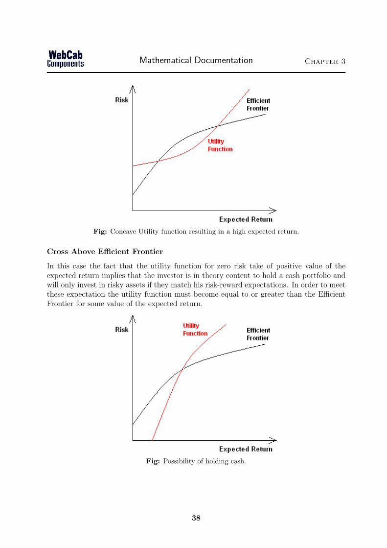
Mathematical Documentation Chapter 3
Fig: Concave Utility function resulting in a high expected return.
Cross Above Efficient Frontier
In this case the fact that the utility function for zero risk take of positive value of theexpected return implies that the investor is in theory content to hold a cash portfolio andwill only invest in risky assets if they match his risk-reward expectations. In order to meetthese expectation the utility function must become equal to or greater than the EfficientFrontier for some value of the expected return.
Fig: Possibility of holding cash.
38

Mathematical Documentation Chapter 3
Utility Function as a function of Risk
The following example was included to illustrate how the methods provided within the:Portfolio:SolveFrontier: class allow the use of utility functions which are functions of risk(rather than the expected return). What this means in practice is that you are able toinvestigate the investors risk-reward profile by asking the required expected return for alevel of risk. If the investors provides this information for a range of values of the risk thenyou will be able to construct the (risk) utility function. We use the term ‘(risk) utilityfunction’ because by collection the investors profile in this form we are only certain thatthe result utility function will be a function in risk. That is, given a value of the risk overthe range for which the Utility function is given there exists a unique corresponding valueof the expected return. However, if we select a value of the expected return there may notexist a corresponding unique value of the risk of the utility function constructed by thismeans.
In the following diagram we provide a example of a (risk) utility function).
Fig: (risk) Utility Function
3.5 Capital Asset Pricing Model (CAPM)
3.5.1 Overview
The CAPM allows the investors portfolio to be constructed from risky assets and ‘cash’holdings or borrowings which are either lent or borrow from the market at some prevailingrate. These additional options of allowing the portfolio to either borrow or lend cash at aprevailing market rate accurately reflects the possibilities available and practices used withthe management of portfolios. That is, when a managed portfolio has excess capital it willtypical be lent to the market at the prevailing rate (which is typically around LIBOR).
39
Mathematical Documentation Chapter 3
Conversely, if the portfolio wishes to increase its positions (and hence expected return)above the capital available within the fund then it will often borrow money at approxi-mately the prevailing market rate (which is typically around LIBOR).
Remark The CAPM simplifies the situation in that it does not take into effect thecredit worthiness of the fund when it wishes to borrow cash from the market. However,the assumptions are not unreasonable if we assume that the fund does not become veryleveraged, since the fund could in principle at least arrange repo agreements which wouldallow it to borrow additional capital at close to the prevailing market rate.
Comparison of CAPM with Markowitz Model
The Capital Asset Pricing Model (CAPM) is an extension of the Markowitz Model. That is,within the construction of the CAPM we assume all the assumption of the Markowitz Model(see 3.1.1) but in addition the investor has the following two options when constructing aportfolio:
1. Lend excess capital at the Market Rate: The investor may lend money at theprevailing market rate. This constitutes the ability to hold within the portfolio arisk free asset which will provide the prevailing return available on cash. In practice,such assets are often referred to as a money market accounts and will yield a returnin the region of LIBOR.
2. Borrow capital at the Market Rate: The investor may borrow money from themarket at the prevailing market rate in order to invest within (risky) assets. Thiswill increase the expected return of the original capital base and also increase itsrisk. In practice, the rate at which money can be lent from the market by a fund willbe in the region of LIBOR (at least if the fund structure the loan as a REPO typeagreement).
Remark Note that the rate of which money can be borrowed or lend from or to themarket is the same.
The similarity of the assumptions of the two models are reflected in there development.In particular, the Efficient Frontier in the sense of Markowitz Theory also plays in centralrole within the CAPM. In the following section we will explain why the optimal portfoliowhich in the Markowitz Theory consisted of a locus (i.e. curve) have been transformed tolie of a line in the case of CAPM.
3.5.2 Nature of the Capital Asset Pricing Model (CAPM)
The introduction of the risk free asset, namely cash along with the risky assets transformsthe ‘curve’ on which the optimal portfolios found with respect to the Markowitz Theoryinto a straight line, known as the Capital Market Line (CML) on which the optimal port-folios with respect to the CAPM lie. The reason for this is that in all cases in order toobtain the optimal portfolio with respect to the CAPM, that is the portfolio which offers
40

Mathematical Documentation Chapter 3
a given return for the minimal risk. You will need to construct a portfolio which consistsof a ‘weighting’ of the ‘Market Portfolio’ (explained below) and either lend excess cashto the market or borrow cash from the market in order to purchase more (baskets) of theMarket Portfolio.
The Market Portfolio is the portfolio on the Efficient Frontier in the sense of MarkowitzTheory (see 3.4.2) which offers the greatest return per unit of risk. Expressing this analyt-ically the Market Portfolio is the portfolio on the Efficient Frontier which maximizes:
Expected Return of the Portfolio
Total Risk of the Portfolio
The reason for this is that the investor whatever his risk/reward profile will seek the port-folio which offers the greatest return of a given level of risk, or the minimum risk for agiven level of return. Clearly, at the level of the expected return of the Market Portfo-lio, the Market Portfolio itself is the optimal portfolio. However, if you wish to obtaina portfolio with a higher expected return then you should borrow cash (with zero risk)from the market in order to purchase more (baskets) of the ‘Market Portfolio’. Since theMarket Portfolio is the cheapest way in terms of risk to increase the return of the portfolio.Similarly, if you wish to obtain a portfolio with a lower expected return than the MarketPortfolio. You will need to hold a sufficient weighting of the Market Portfolio in order thata portfolio consisting of a weighting of the Market Portfolio with the remaining capitalheld as (zero risk) cash holdings will ensure the desired level of the expected return. Againthe rationale for this construction is that the cheapest way to increase the expected returnof a portfolio invested in cash is to move some of the cash into the Market Portfolio whichby definition offers the cheapest means with regard to risk in obtained a higher expectedreturn.
Therefore, when selecting the optimal portfolio with respect to the CAPM one of threepossible scenarios will occur:
1. Borrow money at the prevailing market rate in order to purchase further blocksof the Market Portfolio. That is, the portfolio which offers the greatest expectedreturn per unit of risk. Since the cash borrowings are risk free and unlimited youcan in principle hold an arbitrarily large amount of the Market Portfolio using thesame (original) capital base. Allowing the portfolio to be geared to a level where arearbitrarily high value of the expected return can be obtained.
2. Lend Money at the prevailing rate if you do not require the level of expected returnwhich is offered by investing all the available capital in the Market Portfolio. Thatis, the portfolio with the highest expected return per unit of risk. The rationalebeing that even if you require a lower level of expected return a weighted portfoliobetween the cash with zero risk (and a positive return) and the most efficient meansto purchasing additional expected return (i.e. the Market Portfolio) is going to bemost efficient means of obtaining the desired level of the expected return.
41

Mathematical Documentation Chapter 3
3. No cash holdings or borrowing: if the expected return (or risk) you require isthe same as the expected return (or risk) of the Market Portfolio.
The line within the risk/reward plain which replaces the Efficients Frontier of MarkowitzTheory is known as the Capital Market Line (CML). Where each point on the CMLcorresponds to an optimal portfolio (i.e. minimum risk for a given value of the expectedreturn) with respect to the CAPM.
3.5.3 Applying the CAPM
Since the optimal portfolios with regard to the CAPM all lie on the CML within applica-tions we will nearly always proceed along the following lines:
1. Construction of the Efficient Frontier
2. Evaluation of the Market Portfolio
3. Constructing the CML
4. Selecting a Portfolio from the CML
Construction of the Efficient Frontier
The implementation of the construction of the Efficient Frontier for the CAPM followsalong exactly the same lines as the implementation provided for the Markowitz Theoryand we refer the reader to the earlier section 3.4.2 for general advice concerning the settingof constraints and other issues effecting the construction of the Efficient Frontier. Thoughthe techniques used within the construction does following along similar lines within theimplementation of the CAPM we have only exposed the functionality necessary for theapplication of CAPM. In particular, you will find the followings two methods within the:Portfolio:CapitalMarket: class:
1. :Portfolio:CapitalMarket:setConstraints: - Sets of the constraints (lower and upperbounds) on the assets within the collection of (risky) assets from which the marketportfolio and the other portfolios on the Efficient Frontier will be evaluated.
2. :Portfolio:CapitalMarket:calculateEfficientFrontier: - Evaluates a finite number ofpoints on the Efficient Frontier of the collection of assets from which the marketportfolio can be constructed and store them within a private field. It is necessaryto evaluate the Efficient Frontier because by definition the Market Portfolio is theportfolio on the Efficient Frontier which offers the maximum expected return per unitof risk.
Remark In order to make a more detailed study of the Efficient Frontier we refer you tothe methods contained within the Markowitz class.
By applying these two methods the Efficient Frontier is constructed as follows:
42

Mathematical Documentation Chapter 3
1. Evaluated the Efficient Frontier at a finite number of points. That is, find the port-folio which exhibits the lowest risk for a given expected return from the collection ofasset available. Note that the weights of the assets may be subject to constraints.
2. Interpolate about these points using cubic spline (or some other method) in orderto construct the Efficient Frontier. Since the Efficient Frontier by nature is ‘smooth’using cubic spline interpolation to construct the Efficient Frontier will not introducesignificant errors.
The points on the Efficient Frontier are portfolios constructed from the set of assets con-sidered which exhibit the lowest risk for a given expected return. These portfolio arecharacterized by the following three characteristics:
1. Expected Return - The expected return of the portfolio which is estimated from thehistorical returns of the assets within the portfolio.
2. Total Risk - The total risk of the portfolio which is estimated from the historicalreturns of the assets within the portfolio.
3. Asset Weights - the weights of the collection of assets from which the portfolio canbe constructed.
It is important to point out that the Efficient Frontier in monotonically increasing functionin risk and expected return. This means that if we are given a value of the expected returnthen there will correspond a unique portfolio on the Efficient Frontier with a given totalrisk. Conversely, if we are given the total risk of the portfolio then there will exist a uniqueportfolio on the Efficient Frontier with a corresponding value its expected return.
Evaluation of the Market Portfolio
The Efficient Frontier is the collection of portfolios constructed from the given set of avail-able assets. These portfolios have the lowest risk for a given value of the expected returnwith the possibility of constraints on the weights of the assets.
Once the Efficient Frontier has been constructed are next aim within the application of theCAPM is to find which portfolio on the Efficient Frontier which is the Market Portfolio.That is, the portfolio on the Efficient Frontier which maximizes:
Expected Return of the Portfolio
Total Risk of the Portfolio
The Market Portfolio is selected from the Efficient Frontier using the method :Portfo-lio:CapitalMarket:marketPortfolio:, which will return the (possibly constrained) weights ofthe Market Portfolio which has the highest expected return per unit of risk of the portfolioson the Efficient Frontier constructed from the available set of (risky) assets.
43
Mathematical Documentation Chapter 3
Uniqueness of the Market Portfolio
Here we discuss the ‘uniqueness’ of the market portfolio subject to some remarks concern-ing the given collection of assets from which the portfolios of the Efficient Frontier areconstructed. These remarks though assisting in a deeper understanding of CAPM (andMarkowitz Theory) can be safely skipped for those solely interested in the application ofthe CAPM (or Markowitz Theory).
The uniqueness of the Market Portfolio depends in the nature of the collection of as-sets from which the Efficient Frontier is constructed. Clearly the Efficient Frontier isconvex and hence if we assume that there are two (or more) distinct Market Portfoliosthen it follows that one Market Portfolio is a leveraged version of the other in the follow-ing sense. The covariance between the two (distinct) market portfolios must be one sinceotherwise by holding a weighting of both market portfolios and gaining from the effectsof diversification we are able to construct a portfolio with a higher expected return perunit of risk. Therefore, the covariance between any distinct Market Portfolios must be one.
In fact, if there are two distinct market portfolios with differing values of the risk andexpected return then there exists an continuous range of Market Portfolios (i.e. an infinitenumber) in risk and expected return within the intervals of the risk and expected returnof the two given Market Portfolios. The reason for this is that we can form a weight-ing of the two Market portfolios which forms another Market Portfolio (i.e. it has thesame expected return per unit of risk) which has any value of the expected return or riskwithin there respective intervals. This possibility becomes clear if we consider the portfolioR = aP + (a − 1)Q, where a lies in the interval [0, 1], and where P, Q are the two givenMarket Portfolios. Now as a varies from 0 to 1 the portfolio R’s expected return and riskwill vary over all values within the respective domains but the expected return per unit ofrisk will remain fixed. That is, they will all be Market Portfolios.
Constructing the CML
The Capital Market Line (CML) is simple the line within the risk - expected return plainwhich passes through the Market Portfolio and cash. Below we derive formulae for theconstruction, expected return and risk of an arbitrary portfolio on the CML. We also referthe reader to the diagram of the CML at 3.5.4 which is probably to quickest and easiestmeans to obtain a better understanding on the CML and its construction.
Expressing this analytically: If we construct a portfolio from a (positive or negative)weighting of cash (C) where the prevailing market rate on lending and borrowing cashis r, and the Market Portfolio (M) for a given collection of (possibly constrained) assetsdenoted by M with an expected return of E(M) and risk of R(M), then all portfolios (P )on the CML will take the following form:
P = xcashC + xmarketM
44

Mathematical Documentation Chapter 3
where xcash + xmarket = 1; with the real numbers xcash, xmarket denoting the weighting ofcash and the Market Portfolio within the constructed portfolio on the CML P .
The expected return E(P ), of the constructed portfolio P is given by:
E(P ) = xcashR + xmarketE(M)
where as mentioned above R is the return on cash and E(M) is the expected return of theMarket Portfolio, and where again xcash +xmarket = 1; with the real numbers xcash, xmarket
denoting the weighting of cash and the Market Portfolio within the constructed portfolioon the CML P .
Similarly, the risk σP , of the portfolio P is given by:
σP = (1− xcash)σm = xmarketσm
where σm is the risk of the Market Portfolio, and where again xcash +xmarket = 1; with thereal numbers xcash, xmarket denoting the weighting of cash and the Market Portfolio withinthe constructed portfolio on the CML P .
Remark With the :Portfolio:CapitalMarket: class we provide methods by which theexpected return and risk of the Market Portfolio can be constructed. Moreover, we alsooffer within this class means by which the weighting of the Market Portfolio of an arbitraryportfolio on the CML can be found. In fact, in turns out (see 3.5.3) that if we know anyone of the expected return, risk or Market Portfolio weighting of a portfolio on the CMLthen we are able to deduce the other two properties.
Selecting a Portfolio from the CML
The Capital Market Line (CML) is a collection of portfolios which can be constructed fromthe available (risky) assets with the option of borrowing or lending (risk free) cash at theprevailing market rate. Since by default the amount of cash which can be borrowed orlend is not restricted the expected return of the resulting portfolios can be anything equalor greater than the return available from cash. Similarly, the risk from possible portfolioscan (by default) be any positive number.
We allow within this Component the portfolios on the CML to be selected from knowledgeany one of the following:
1. Expected Return
2. Total Risk
3. Weighting of the Market Portfolio
This in fact allows for the greatest generality and moreover which even property is used inthe identification the other two properties can be deduced as described below.
45
Mathematical Documentation Chapter 3
Completeness of the Methods: riskCML, weightCML, returnCML, weight2Riskof the CapitalMarket class
The portfolio on the CML can be selected when one of the following three properties isknown:
1. Total Risk of the optimal portfolio on the CML.
2. Expected Return of the optimal portfolio on the CML.
3. Weighting of the market portfolio on the CML.
Then using the above mentioned methods we are able to evaluate the other (two) quanti-ties from the three properties which are listed above. For example, if the expected returnof the portfolio is known then the weight of the market portfolio can be evaluated usingweightCML and the risk can be evaluated using riskCML. If on the other hand the totalrisk of the portfolio is known then the corresponding expected return of the portfolio canbe evaluated by returnCML, and then using this deduced value we are able to evaluated theweight of the market portfolio using weightCML. For completeness we include the methodweight2Risk which evaluates the risk of a portfolio on the CML when the weight of themarket portfolio within the CML portfolio is known. From knowledge of the risk of theCML portfolio we able to evaluate the corresponding value of the expected return usingthe method returnCML.
Therefore, using the three ‘. . .CML’ methods along with ‘weight2Risk’, which ever oneof: total risk, expected return or weight of market portfolio, is used in order to selectthe optimal portfolio from the CML we are able to deduce the other two quantitativeproperties.
3.5.4 Summary of the CAPM
We summarize the CAPM with the following diagram which contains the Efficient Frontier(the black curve) which is first evaluated, then the Market Portfolio (denoted by a redsquare) is found on the Efficient Frontier. After which when ‘cash’ (denoted by red squareon Expected return axis) we are able to construct the CML (red line) by drawing a linethrough cash and the Market Portfolio.
46

Mathematical Documentation Chapter 3
Fig: The CML, Market Portfolio, and the Efficient Frontier
The gray perpendicular lines on the diagram running off from the Market Portfolio indicatesthe values of the risk and expected return of the Market Portfolio. Any portfolios to theleft on the risk axis to the Market Portfolio on the CML are portfolio which borrow cashfrom the market. Similarly, any portfolio to the right on the risk axis on the CML areportfolio which lend cash to the market. In a similar fashion, any portfolios on the CMLwith an expected return greater than the Market Portfolio (i.e. above the gray horizontalline) borrow cash from the market, and any with a lower expected return (i.e. below thegray) lend cash to the market.
3.5.5 Putting constraints on the level of borrowing and lending
At present we are able to place constraints on the weights of the (risky) assets from whichthe portfolios on the Efficient Frontier used within the Markowitz Theory and CAPM canbe evaluated. This allows the risky asset held within the portfolios on the Efficient Frontierfrom which in the case of Markowitz Theory the optimal portfolio will be selected. Hence,within the framework on Markowitz Theory we have a means by which to place constraintson all the assets of the optimal portfolio.
In the case of the CAPM, a portfolio can also contain either cash holdings (i.e. free riskassets yielding the prevailing market rate on cash) or borrowings (i.e. money borrowedfrom the market at the prevailing market rate). Are aim here is to rationalize and detail
47

Mathematical Documentation Chapter 3
the issues related to why and how constraints can also be placed on the cash holdings orborrowings.
Rational of Borrowing Limit
Within the mandate of a fund, the manager will often be set a maximum amount of gearingwhich the fund can take. If the manager ever wishes to go above this level then they willneed to obtain authorization from the funds board.
From the point of view of risk management and hence credit rating and regulation. Ifthere is maximum level of gearing then there is a worst case scenario otherwise the worstcase scenario since the gearing is unlimited is unlimited losses.
Rational for a Cash Limit
The existence of a cash limit forces the fund to invest within the market which it addresses.The primary motivation for introduction such a limit are as follows:
1. Role of a Fund Manager: A portfolio manager to paid to invest money by selectingassets within a given sector or market. After all if the money is just deposited within abank account the fund manager will still collect the management fee without reflectinghis mandate. The mandate explicitly said invest in... If the investor wants to be outof the market then they can take money out of the fund.
2. Reflect fund description/mandate: An equity fund should not be a money mar-ket fund. I.e. Having limit like no more the 40% in cash at any time is reasonable.If this is not possible then capital should be returned to investors for similar reasonsas within any other business.5
Mechanics of controlling the Cash/Borrowing Level
Within the CAPM the optimal portfolios which are constructed from a combination of theMarket Portfolios with the possibility of cash holdings or borrowings lie on the CML. Ifthere is a pre-defined limit on the level of cash holdings or borrowings then these limitswill translate into a limit on the weighting the Market Portfolio within the portfolio ofthe CML. From limits on the weighting we will be able to imply the limits on the risk, orexpected returns of the portfolio on the CML which satisfies the cash and borrowing limitssince as shown above if one of the following three: weighting, risk, expected return; areknown then the other two can be deduced.
5For further discussion on the effect of retaining earners and compounding we refer the invested readerto; The Essays of Warren Buffet, Lessons for Investors and Managers, edited by L.Cunningham.
48
Mathematical Documentation Chapter 3
Implemented as an Example
We provide within this package a client example which illustrates how constraints on thelevel of cash lending or borrowing can be used. The client is entitled:
CapitalMarketClient CashConstraints
This example illustrate how constraints may be placed onto the levels of the cash heldor borrowed to the market by an optimal portfolio constructed in accordance within theCapital Asset Pricing Model. We show how the resulting continuous range of the valuesof the expected return and total risk can then be deduced which identify which optimalportfolios can be selected when the cash level constraints are observed.
In particular we consider the following problem:
We know that the market portfolio of a collection of assets has an expectedreturn of 10 percent per year and a risk of 20 percent per year, we also knowthat cash can be borrow or lend from the market at a prevailing rate of 5 percenta year. According to the CAPM if the portfolio manager can only leverage hisportfolio by 20 percent, and must also never hold more than 30 percent of thefunds capital in cash then what is the range of total risk and expected returnof the (optimal) portfolios which the fund manager can hold?
3.6 Performance Evaluation
As we discussed earlier since there is a relation between the risk and the expected returnfrom an asset (CAPM) an assessment of a portfolios performance based only on the abso-lute return is misleading and unfair. Therefore, we describe standard methods which areused to given a risk adjusted performance measure.
Within the US mutual fund market there are more than 12,000 funds which apply a varietyof investment styles and have a different mix of investment assets. Broadly speaking USmutual funds can be split into the following categories growth funds, balanced funds, in-come funds, government bonds funds, junk bond funds and international funds. Accordingthe CAPM the investors would expect a greater return from a growth fund which investsin stocks than a government bond fund because the growth fund will exhibit more volatil-ity. The amount of “out performance” of the growth fund over the bond fund which theinvestor would expect is the topic of this section.
We offer various methodologies which are used for the evaluation of portfolio performancein the broad sense. These measures are widely used and offer a fast and efficient way inorder to make informed comparisons between portfolio performance taking into accountrisk, return, asset class mix, yield and market conditions.
Within our components we implement the following methods:
49
Mathematical Documentation Chapter 3
• totalReturn - calculates the total return of the portfolio over a given period takinginto account any disbursements and dividends payments
• geometricMeanReturn - the geometric mean of the return over a number of periods.Say the return is quoted for a 2 year period then by taking the number of periods as2 the method will return the equivalent return over a 1 year period
• sharpesRatio - we implement Sharpe’s ratio which takes into account both thereturn and risk when accessing a portfolios performance
• treynorsMeasure - Treynor’s performance measure which takes into account the sys-tematic risk (or beta) and the average return when assessing the overall performance
3.6.1 Comparing the Sharpe and Treynor Performance Measures
The Sharpe portfolio performance measure is based on the capital market line (CML) andtotal risk, which makes it more suitable for evaluating portfolios rather than individualassets. On the other hand, Treynor performance measure is based on the capital assetpricing model (CAPM) and are more flexible because by using systematic risk (beta) itcan be used to evaluate the performance of both portfolios and individual assets. Bothperformance measures tend to rank a group of diversified portfolios similarly.
3.7 Further and Supplementary Reading
3.7.1 Supplementary Reading
• H. Markowitz Portfolio Selection, Journal of Finance, 1952, p77-91
This fundamental paper establishes the basis of the Markowitz theory andshows that portfolios dominate individual assets from a risk and returnstandpoint. Further it shows how to construct optimal portfolios withideal risk - return characteristics.
3.7.2 Further Reading
• H. Markowitz Portfolio Selection, Efficient Diversification of Investments, BasilBlackwell
Expands on the classic 1952 article listed above detailing the modern treat-ment and development of the theory.
• W. Sharp A Simplified Model for Portfolio Analysis, Management Science, Vol. 9,p27-93
50

Chapter 4
Programmer’s Guide
This chapter describes development techniques for various business solutions that make use ofthe functionality provided by our J2SETM Component. We analyze both standard and enterpriseJava solutions including stand-alone Java applications, Java Applets, JSP pages and EnterpriseJavaBeansTM .
4.1 Developing with J2SE
The J2SE Edition of this product offers core-level functionality to the Java developer al-lowing the implementation of fully personalized components and applications for specificbusiness problems on a variety of deployment environments. Irrespective of the complexityof the project a programmer may be working on, this J2SE Component can be integratedin an equally straightforward manner by providing the needed functionality in a compactand precise way.
The Portfolio v4.2 component comes wrapped inside a Java JAR file called PortfolioJ2SE.jar.This class library contains all classes that provide the functionality offered by this J2SEComponent as documented inside the API reference directory of this package (/JavaDocs).Depending on the type of Java solution you are developing, you will be using this JARfile in a specific way. Once you have chosen a particular implementation of a deploymentframework, the structure of your source code will need to adapt accordingly. In the follow-ing discussion we describe several basic J2SE implementation examples that can be usedto make use of our product’s functionality.
4.1.1 Stand-alone Java Applications
A stand-alone Java application is a Java class which acts as a client for any type of Javacomponents ranging from JavaBeans, class libraries and EJB components. The source codelisted below defines a standard stand-alone application skeleton which communicates witha class within a J2SE Component. By creating an instance, calling a method, sending ina set of parameters and then retrieving the returned result of the method call. As soonas the method call has gone through successfully the method continues by displaying its
51

Programmer’s Guide Chapter 4
result on the screen.
/*
* The class we are using is located in the webcab.lib.j2sepackage package.*/
import webcab.lib.j2sepackage.*;
public class StandAloneExample {
public static void main (String[] args) {
/*
* Creates an instance of the J2SEClass class*/
J2SEClass instance = new J2SEClass ();
/*
* Defines the method parameter.*/
double parameter = 25;
/*
* Invokes a method with the specified parameter* and puts the result in the result variable.*/
double result = instance.computeResult (parameter);
/*
* Prints out the retrieved result.*/
System.out.println ("Method ’computeResult’ in class J2SEClass
returned " + result + ".");
}
}
If the method computeResult of the J2SEClass class returned 100, this stand-alone ap-plication would print the following:
Method ’computeResult’ in class J2SEClass returned 100.
52

Programmer’s Guide Chapter 4
4.1.2 Java Applets
Applets run within a Java enabled web container allowing real-time user interaction onthe Internet. The source code listed below defines an Applet which performs the samecalculations as the stand-alone example above and then graphically displays the result.
/*
* The class we are using is located in the webcab.lib.j2sepackage package,* while the Applet specific classes reside in javax.swing.*/
import webcab.lib.j2sepackage.*;
import javax.swing.*;
public class AppletExample extends JApplet {
public void init () {
/*
* Creates an instance of the J2SEClass class*/
J2SEClass instance = new J2SEClass ();
/*
* Defines the method parameter.*/
double parameter = 25;
/*
* Invokes a method with a specified parameter* and puts the result in the result variable.*/
double result = instance.computeResult (parameter);
/*
* Prints out the retrieved result.*/
getContentPane ().add (new JLabel ("Method ’computeResult’ in
class J2SEClass returned " + result + "."),
java.awt.BorderLayout.CENTER);
}
}
53

Programmer’s Guide Chapter 4
This Applet source code will be compiled and placed together with all classes from thePortfolioJ2SE.jar file in another Java JAR file and be deployed inside a web container.Users connecting through a web browser will first download this newly created Java JARfile and then interact with the Applet’s graphical interface.
4.2 J2EETM Solutions Using J2SE Components
The JavaTM2 Enterprise Edition platform provides a great variety of business frameworksolutions, which transfer hard-coding to the Application Server providers and enables thedeveloper to exclusively concentrate on the business problem. In the following sections wediscuss two of the most popular J2EE technologies, Java Server Pages (JSP) and EnterpriseJavaBeans (EJB), which are universally supported by all Application Server providers.
4.2.1 Writing JSP Pages
JSP Pages are very much like Applets since they both basically offer the same functionalityto the end-user, interaction within a web page. But even though they both display theirresults in a browser, the main difference is the fact that JSP pages are server-side applica-tions, which never get downloaded onto the client’s machine and never use local CPU ormemory resources. Yet as previously stated the code you will write when designing yourJSP pages to use our J2SE Components will be very similar to client side applications wehave already described. That is, you will need to make the following steps:
• Create an instance of the class you wish to use
• Make a method call by sending the required parameters
• Display the result in HTML form
54

Programmer’s Guide Chapter 4
The following JSP page exemplifies this process:
<!-- The class we are using is located in the webcab.lib.j2sepackage package.-->
<%@page import="webcab.lib.j2sepackage.*"%>
<HTML>
<HEAD><TITLE>JSP using J2SE Component Example</TITLE></HEAD>
<BODY>
<%
/*
* Creates an instance of the J2SEClass class*/
J2SEClass instance = new J2SEClass ();
/*
* Defines the method parameter.*/
double parameter = 25;
/*
* Invokes a method with the specified parameter* and puts the result in the result variable.*/
double result = instance.computeResult (parameter);
%>
<!-- The JSP page displays the result inside the web browser. -->
Method ’computeResult’ in class J2SEClass returned <%=result%>.
</BODY>
</HTML>
The JSP page will be compiled into an HTML page by the web container on the serverand be served to the client’s machine where the end-user will be able to read the computedresult, as if it had been run locally.
4.2.2 Designing EJBTM Components with J2SE Components
Enterprise JavaBeansTM are server-side components which provide the same business func-tionality as J2SE Components while not taking up local system resources. Developerswriting EJB components that use the functionality provided by J2SE Components willneed to include the PortfolioJ2SE.jar file with their enterprise deployment archive (EAR)and perform local calls like shown in the previous examples. The following source code de-fines the implementation class of a stateless Session Bean which makes calls to a J2SE class.
55
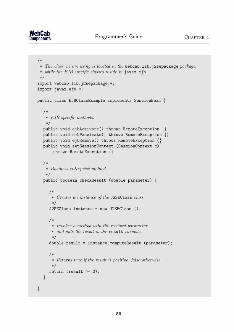
Programmer’s Guide Chapter 4
/*
* The class we are using is located in the webcab.lib.j2sepackage package,* while the EJB specific classes reside in javax.ejb.*/
import webcab.lib.j2sepackage.*;
import javax.ejb.*;
public class EJBClassExample implements SessionBean {
/*
* EJB specific methods.*/
public void ejbActivate() throws RemoteException {}public void ejbPassivate() throws RemoteException {}public void ejbRemove() throws RemoteException {}public void setSessionContext (SessionContext c)
throws RemoteException {}
/*
* Business enterprise method.*/
public boolean checkResult (double parameter) {
/*
* Creates an instance of the J2SEClass class*/
J2SEClass instance = new J2SEClass ();
/*
* Invokes a method with the received parameter* and puts the result in the result variable.*/
double result = instance.computeResult (parameter);
/*
* Returns true if the result is positive, false otherwise.*/
return (result >= 0);
}
}
56

Programmer’s Guide Chapter 4
Together with its home and remote interfaces this class will encapsulate a stateless SessionEJB that serves client-side requests by making local J2SE calls.
Remark For further details concerning the use of this component as an EJB, pleasesee the Programmers Guide of the J2EE Editions PDF documentation.
4.3 Using JDBC Mediator with our J2SE Components
4.3.1 Overview
The JDBC mediator is a J2SE Component which mediates between a J2SE Component,its clients, and DBMS. For each J2SE Component there exists a corresponding mediatorwith its own exception class. The mediator receives an input and an output SQL queryfor the DBMS and a method name to analyze. The mediator sends the SQL input queryto the (input) DBMS and then applies the method from the J2SE Component to each rowof the input query results. Each result row is written into the (output) DBMS accordingto the output SQL query.
A diagram that illustrates how JDBC Mediator intermediates the communication between the J2SE
client, the J2SE Component, and the Database Servers.
4.3.2 Connecting to your Database Server
If you wish to connect by JDBC to your Database server in order to run a select queryan update statement or a stored procedure you will need to describe the connection withcertain properties.
57

Programmer’s Guide Chapter 4
• DriverThe driver is a Java class provided by your Database vendor that implements thejava.sql.Driver interface.
• URLThis property defines the address of your DBMS, the port number and additionalinformation such as service and database name.
• Username and PasswordFor authentication reasons, most connections will not work without providing a username and a password.
• Additional PropertiesThis field allows you to customize even more your JDBC connection as described inthe JavaDocs
We describe these properties individually for best known database systems. Please feel tojump to the section which refers to the particular DBMS you plan to use with our J2SEJDBC Components.
Oracle 9i
We recommend the JDBC thin driver oracle.jdbc.driver.OracleDriver. You maydownload this driver from http://otn.oracle.com/software/tech/java/sqlj jdbc/content.html.The Oracle URL has the following format:
jdbc:oracle:thin:@servername:port:service
where servername is the Internet name of your Oracle DBMS, port is usually 1521 andservice is the name of the service you are going to connect to.
IBM DB2
The name of the DB2 driver is COM.ibm.db2.jdbc.net.DB2Driver and can be down-loaded off the IBM site at http://www-3.ibm.com/software/data/db2/java. The format ofthe DB2 URL is:
jdbc:db2://[servername]:[port]/[database]
where servername is the Internet name of your DB2 DBMS, port may be ignored anddatabase is the name of the database you plan to connect to.
Microsoft SQL Server
The name of the SQL Server driver is com.microsoft.jdbc.sqlserver.SQLServerDriverand can be downloaded off the Microsoft site at http://msdn.microsoft.com/.... The for-mat of the Microsoft SQL Server URL is:
58

Programmer’s Guide Chapter 4
jdbc:microsoft:sqlserver://servername:1433
where servername is the Internet name of your SQL Server.
Sybase
The name of the Sybase driver is com.sybase.jdbc.SybDriver and can be downloaded offthe Sybase site at http://www.sybase.com/home. The format of the Sybase JDBC URL is:
jdbc:sybase:Tds:servername:port/
where servername is the Internet name of your Sybase DBMS and port is the port numberwhere the Sybase server is running.
4.3.3 J2SE JDBC Components
Most methods implemented by our components accept numeric parameters and returnnumbers or arrays of numbers. The JDBC Mediator enables these methods to take theirnumeric parameters from a Database server and return the numbers by writing them backinto the same or another Database server.
The following modules within this J2SE Component implement the JDBC Mediator func-tionality:
• The ‘Portfolio’ package
For every class implementing number-based methods (methods with numeric parametersand numeric return values) there’s a class in a sub package called “jdbc” bearing a sim-ilar name. For example, if there’s a class called “Volatility” within a package called“webcab.lib.finance.options”, the corresponding J2SE JDBC class would be named“webcab.lib.finance.options.jdbc.VolatilityJDBC”.
A J2SE JDBC class may be instantiated by specifying all necessary JDBC connectionparameters, such as drivers, url, username and password plus the constructing parametersof the underlying J2SE class. Every J2SE JDBC class contains several methods that invokemethods from its underlying J2SE class and apply them directly to your Database tablesand/or write the answer back into the same or another Database. These J2SE JDBCmethods accept the name of the method as the first parameter and an SQL Query or anarray of Java objects for the method’s input and output.
The following source code listing illustrates how to use an input/output SQL query JDBCmethod for a generic J2SE class “webcab.lib.finance.FinancialClass” and a genericmethod “double calculateAmount(double, double)”.
59

Programmer’s Guide Chapter 4
import webcab.lib.finance.*;
import webcab.lib.finance.jdbc.*;
...
try {...
/*
* The first construction parameter (riskFreeInterestRate) is FinancialClass* specific. The next parameters define the input and the output* DBMS connections by driver, url, username, password and additional* properties.*/
FinancialClassJDBC jdbcMediator = new FinancialClassJDBC
(riskFreeInterestRate,
"oracle.jdbc.driver.OracleDriver", // Input Connection
"jdbc:oracle:thin:@inputserver.com:1521:ORACLE",
"SCOTT", "tiger", null,
"oracle.jdbc.driver.OracleDriver", // Output Connection
"jdbc:oracle:thin:@updateserver.com:1521:ORACLE",
"MIKE", "wolf", null);
jdbcMediator.call ("calculateAmount",
"SELECT C ID, SHARES, VALUE FROM TRADES",
"UPDATE CUSTOMER SET MONEY=? WHERE C ID=?",
new int[][] {{2, 1}});catch (Exception e) {e.printStackTrace ();
}
The first parameter of the call method represents the FinancialClass method name.The second parameter is the input query, a select query which returns three columns C ID,
SHARES and VALUE. The third parameter is a prepared statement that is meant to write thevalue returned by calculateAmount in the MONEY field and the C ID primary key in thewhere clause. This assignment is described by the last parameter, an array of integer pairsthat specifies the index of the IN parameter in the output query and the column numberof the input query. Both indices start counting from 1. In our case, the second IN param-eter is the second question mark in the update statement and the first input column is C ID.
Every output update is made according to a primary key C ID. Even though this isreturned by the select statement it is not used for computation by the two-parameter“calculateAmount” method.
60

Programmer’s Guide Chapter 4
4.4 The Portfolio J2SE Methods
This component offers portfolio analysis according to Markowitz and Capital Market The-ory. There are two main categories of methods which are provided within this component:
• statistical parameter calculation
• portfolio analysis
The values returned from the first category are used when calling portfolio analysis meth-ods. You can calculate either individual asset parameters (e.g. the expected return froman asset), or portfolio parameters (e.g. the expected return of the portfolio). Usually youwill be interested more in the analysis functions. Almost all of these functions require thecovariance matrix and / or the expected returns vector. You can obtain them by callingcovMatrix, respectively expArray. Also, when calculating statistical parameters, you cangive the probabilities as parameters or you can use an estimation based on historic ratesof return (see 3.1.1 for details).
The most time consuming part of the analysis is the determination of the efficient fron-tier (see 3.4). This requires a series of minimizations, which are done using Rosen’sgradient projection algorithm. Because it is inefficient to do this every time you wantto know the portfolio on the efficient frontier corresponding to a given expected return,the result is determined by interpolating through a series of points. The interpolationpoints must be calculated before a call to efficientFrontier(double, int) is made. Themethod calculateEfficientFrontier does this. If you are interested instead in only onepoint from the efficient frontier, you can use efficientFrontier(double, double[][],
double[], int, double). In order to determine the optimum portfolio (according toMarkowitz model) a utility function (indifference curve) must be provided (see 3.5). Itcan be given either as a set of interpolation points, or as a polynomial (by specifyingcoefficients). Having a utility function and an efficient frontier, you can determine theset of optimal portfolios (i.e. the set of intersection points between the two curves) usingoptimalPortfolio. If you are interested only in one value you can use optimalPortfolioMaxExpectedwhich determines the point in the set with the maximum expected return. The maximumnumber of optimal portfolios found is 100. If this number is exceeded, an exception willbe thrown.
We provide a method for calculating the equity portfolio (see 3.6). This also requiresthe efficient frontier to be calculated.
Remarks You should be aware that there are two sources of errors: the first is theoptimization procedure, the second is the interpolation. Usually the errors generated bythe interpolation are much bigger than that resulting from the optimization. You can re-duce the interpolation errors by increasing the number of interpolation points. It is muchharder to control the optimization errors. If you are especially interested in an accurateresult, you can adjust the ‘portal’ parameter to lower values, otherwise this should always
61

Programmer’s Guide Chapter 4
be set between 1E − 3 and 1E − 6. The ‘projtol’ parameter is not the tolerance of theresult, so there are no guarantees that the error will be less than a specific number. Alsothe increase in duration of the algorithm does not depend linearly on the value of ‘projtol’,so a small decrease of it can cause a great increase in time consumption. Generally, theaccuracy of the result depends on the input data. Usually, the more assets are in theportfolio, the bigger optimization errors are.
4.5 Exceptions
If one of the methods which require the efficient frontier to be calculated is called beforecalculateEfficientFrontier, the exception EfficientFrontierNotCalculatedException
will be thrown.
If one of the methods which require the utility function is called without initializing it,the exception UtilityFunctionNotInitializedException will be thrown.
If the number of optimum portfolios found is greater than 100, the exception TooManyPortfoliosException
is thrown.
The expected return of a portfolio cannot be greater than the maximum expected re-turn of the assets. If you want an expected return higher than this, the problem has nosolutions. So, when calling efficientFrontier with such an expected return, you will geta NoSolutionException . Also if the range given to calculateEfficientFrontier containsany points for which there is no solution, the exception will be raised.
4.6 Support for Developers
4.6.1 Compilation and Custom Modification of Source Code
This J2SE Components source files have been compiled using Sun’s J2SDK1.4.2, shouldyou prefer compilation of the source code using another compiler then please contact us.Some functions (for example standard mathematical operations) are embedded within thesource code, if you license classes which you believe offer a similar level of functionalityfrom a third party and wish to include these classes within our components then pleasecontact us. Both of the above services are offered free of charge at WebCab’s discretion.
4.6.2 Online
Should you have any questions or queries, please feel free to contact us via our supportforum at:
http://www.webcabcomponents.com/support/index.php
For updates and new releases, visit:
62

Programmer’s Guide Chapter 4
http://www.WebCabComponents.com/Java/index.shtml
63
Chapter 5
Examples
Within this chapter we illustrate how the Portfolio Component can be applied to solve reallife problems. We provide with this Component examples of two types:
1. QA Examples
2. Custom Examples
5.1 Question and Answer (QA) Client Examples
5.1.1 Overview
Within this folder we offer Java client examples for the J2SE Business Components providedwithin this package. In particular, for each business method contained within each businessComponent we provide a client side example; which illustrates how functionality containedwithin this component can be applied to solve real world problems. In addition, to theseexamples we also include custom applications which solve some of the generic problemswhich this Component is designed to address.
5.1.2 Structure of QA Examples Directory
By drilling down the QA Client directory structurr you will find the following six directorylevels:
1. Client Level2. Technology Level3. Business Module Level4. Business Class Level5. Example Level6. Custom Example Level
which have the structure as shown in the following diagrams.
64

Examples Chapter 5
5.1.3 Top Four levels of the QA Directory Structure
(Technology Level) (Business Module Level) (Business Class Level)
Client +
|
+ Java -------+
| |
+ Readme.txt + ‘Business Module 1’ -------+
| |
+ ‘Business Module 2’ --+... + ‘Business Class 1’ ----------
| |
+ QALibrary.jar + ‘Business Class 2’ --+...
|
+ ...
5.1.4 Bottom Two levels of the QA Directory Structure
(Example Level) (Custom Example Level)
-----+
|
+ ‘BusinessClass’.java
|
+ compile.cmd (.sh for Linux)
|
+ run.cmd (.sh for Linux)
|
+ run_gui.cmd (.sh for Linux)
|
+ ‘CustomClient’ -----------------+ ‘CustomClient’.java
| |
+ ... + compile.cmd (.sh for Linux)
|
+ run.cmd (.sh for Linux)
5.1.5 Quick Start Guide
Browse down to the particular client within the business module for the given client tech-nology you are interested in. Run the compile.cmd (.sh for Linux), script in order tocompile the example and then run the run.cmd (.sh for Linux), script in order to run theexample.
65

Examples Chapter 5
5.1.6 Explanation of the QA Directory Structure and its files
1. Client Level
The directory containing the Questions and Answer Examples is named ‘QAClients’.This directory can be located by using the Index.html file, which is presented at theend of the installation process, by selecting:
Run Examples > Client Examples Directory
Within this folder you will also find the following file:
• Readme.txt - this readme file
2. Client Technology Level
Within the ‘Client’ folder is the Technology Level of the QA directory structure.Within this folder you will find sub-directories; which contain examples written ineach of the Java Client Technologies in which the clients have been implemented.
As mentioned above within the overview we provide an implementation of each ‘Ques-tion and Answer (QA)’ example using each of the client technologies used. Selectingone of these folders in order to view the client implemented within the correspondingtechnology.
3. Business Module Level
After selecting one of the technology sub-folders at the ‘Client Technology Level’ (see(2) above) you will enter a folder which contains a sub-folder for each of the modulescontained within this component package. The modules are convenient collectionsof business classes containing the business functionality offered by this component.Each module has a sub-folder which contains the ‘Question and Answer’ examples ofeach method of the classes which it contains.
This directory will also contain the following file:
• QALibrary.jar - contains utility functionality necessary for running the clients.
4. Business Class Level
At the business class level under the module level we are presented with one sub-folderfor each of the classes within the business module. Each of these folders contains thefiles of the examples for each of the methods contained with the respective class.
5. Example Level
At the Example level you will be presented with the files which allow you to compile
66

Examples Chapter 5
and then run the examples of the application of the Business methods of the respec-tive class. The files within this directory which constitute the Client example are asfollows:
• Source Code File(s) - Depending on the Java compatible technology selected atthe ‘Technology Level’ this folder will contain a source code file(s) of the client.
• Compile Batch File - Assuming that you have access to the relevant compilerthe compile batch file (compile.cmd or compile.sh) once run will compile theclient example from the folders source code file. Below we include some remarkson how to obtaining suitable Java compiler in order to be able to compile andthen run the Java examples.
• Run Batch File - The run batch file (run.cmd or run.sh) will run the examplesexecutable file (exe) which is generated from the compilation of the source codefile. If the example over runs your console screenful then press space in orderto page down or enter is order to scroll down.
6. Custom Example Level
At the Custom Example level you will find a source code file containing the im-plementation of the Application which addresses a typical question for which theComponent is designed. The source code has a linear structure with full inline com-mentary. By just running the compile and then run scripts contained within thisdirectory you will be able to solve to given problems view the results obtained. Thefiles contained within each Custom Client Example directory are as follows:
• Source Code File(s) - The custom clients source code in the appropriate clienttechnology.
• Compile Batch File - Assuming that you have access to the relevant compilerthe compile batch file (compile.cmd or compile.sh) once run will compile theclient example from the folders source code file.
• Run Batch File - The run batch file (run.cmd or run.sh) will run the examplesexecutable file which is generated from the compilation of the source code file.If the example over runs your console screenful then press space in order to pagedown or enter in order to scroll down..
5.1.7 Remarks on Java compilers
1. Required compilers and how to test for them
In order to compile the Java examples you will require a suitable Java compilerwhich should be installed and configured within your environment variable PATH.The easiest way in which to test whether you have access to a Java compiler at yourcommand prompt is to type the follow command at the command line:
67
Examples Chapter 5
java - Invokes the Java compiler
2. How to obtain the required Java compiler
Compilers for the Java programming language are provided within Sun’s Java SDKwhich can be obtained from:
http://java.sun.com
5.2 Custom QA Examples
Portfolio theory addresses the very practical aim of trying to get the highest expectedreturn from a portfolio for a given level of risk. Within this section we detail the customexamples which we provide with the portfolio components standard QA Example, whichillustrate the application of the Portfolio Component.
5.2.1 Markowitz Custom Clients
Within this section we describe the custom examples which we provide for the Morkowitzclass. The source code for these examples can be found within sub-directories of thedirectory:
Clients > QAClients > “Language/Technology” > Portfolio > Markowitz
where ”Language/Technology” refers the program language and/or technology (for ex-ample Java, C, Delphi, EJB, COM, Web services, CORBA etc) by which the example arewritten in.
1) AbsoluteRelative
This example demonstrates that whether the absolute or relative values are used for thesource data of the historical returns the Portfolio Component will yield the “same” resultsin terms of selecting the optimal portfolio.
In particular, we will show the independence of the Weights of the Portfolio found onthe Efficient Frontier for a given expected return. Moreover, we will show that whether weuse absolute or relative values for the historical returns the weights of the optimal portfoliofound are identical.
One reason for this independence is that the units in which the historical returns are givendoes not effect the weights of the portfolio of the Efficient Frontier, include the weights ofthe optimal portfolio is that asset weights themselves are nit-less’ (in the sense of Measure-ment Theory). Hence intuitively speaking during the computation of the asset weights theunits are being canceled out with the end result (i.e. the weights) being recording withoutan attached unit.
68

Examples Chapter 5
2) Efficient Subdirectory
This example demonstrates how we are able to evaluate a single Portfolio on the EfficientFrontier. That is, we demonstrate how we are able to find any portfolio of the EfficientFrontier with only one call to the underlying Rosen’s optimization algorithm.
In instances when we only require to evaluate a few portfolios on the Efficient Frontierthen this direct approach is not only more efficient but also more accurate.
Level of the Precision
Another aspect of this example is that we show how the portfolio found depends on theprecision used. In particular, we find that a precision of 1E-12 (or higher) should be usedin order to assure that the weights of the portfolio are corrects to 2 decimal places.
Historical Values Used
Within this example we use the following relative historical values of five assets histor-ical returns over the last five periods:
• 1st Asset: 0.03, 0.04, 0.02, 0.05, 0.03
• 2nd Asset: 0.03, 0.040, 0.1, 0.03, 0.035
• 3rd Asset: 0.03, 0.032, 0.033, 0.035, 0.036
• 4th Asset: 0.02, 0.021, 0.021, 0.021, 0.0205
• 5th Asset: 0.02, 0.01, 0.02, 0.015, 0.028
Where the portfolios on the Efficient Frontier can be constructed with respect to thefollowing asset weight constraints:
• 1st Asset Weight Constraints: Lower bound of = 0.05, Upper bound = 0.2
• 2nd Asset Weight Constraints: Lower bound = 0.05, Upper bound = 1
• 3rd Asset Weight Constraints: Lower bound = 0.05, Upper bound = 1
• 4th Asset Weight Constraints: Lower bound = 0.05, Upper bound = 0.5
• 5th Asset Weight Constraints: Lower bound = 0.05, Upper bound = 1
3) Optimal Subdirectory
With this example we select the Optimal Portfolio in accordance with Markowtiz Theoryusing an Investors (risk/reward) Utility Function. Here the returns are given in absoluteterms.
69

Examples Chapter 5
Suppose you have the historic rates of return for 5 assets given in the table:
Month Asset1 Asset2 Asset3 Asset4 Asset5January 100 75 120 50 150February 105 76 120 50 150March 107 76.5 130 50 145April 110 77 130 51 135May 90 70 125 45 120June 75 71 105 46 110July 80 73 105 46 110August 80 75 110 47 170September 90 77 120 48 200October 97 79 120 49 200November 105 78 125 50 205December 115 77 135 51 210
Problem: What are the asset weights of the optimal portfolio which has an expectedreturn of 120?
That is, what are the weights of the 5 assets such that the risk of the resulting portfo-lio is minimized and the return is equal to 120. We have chosen to use a tolerance of 1E−3.
Solution: The reqwuired weights are:
Asset weightAsset1 0Asset2 0.01067Asset3 0.98764Asset4 0Asset5 0.00169
For further details we refer the reader to the source code and in-line documentation of thisexample.
4) Optimal2 Subdirectory
Within this example we will consider the construction the efficient frontier for the portfoliowhich can be constructed from three managed fund with returns of 12 periods of:
• Fund 1: 1.14, 0.47, 0.84, 0.93, 1.1, 0.82, 0.63, 0.72, 0.8, 1.06, 0.79, 0.78
• Fund 2: -6.06, -4.15, 1.37, 4.29, 1.37, -1.21, 4.11, 2.19, -3.71, 1.18, -1.25, 1.29
• Fund 3: -1.7, -4.9, 3.64, 4.14, 1.14, 1.66, 4.18, 4.01, -0.11, 4.24, -2.26, 4.33
70
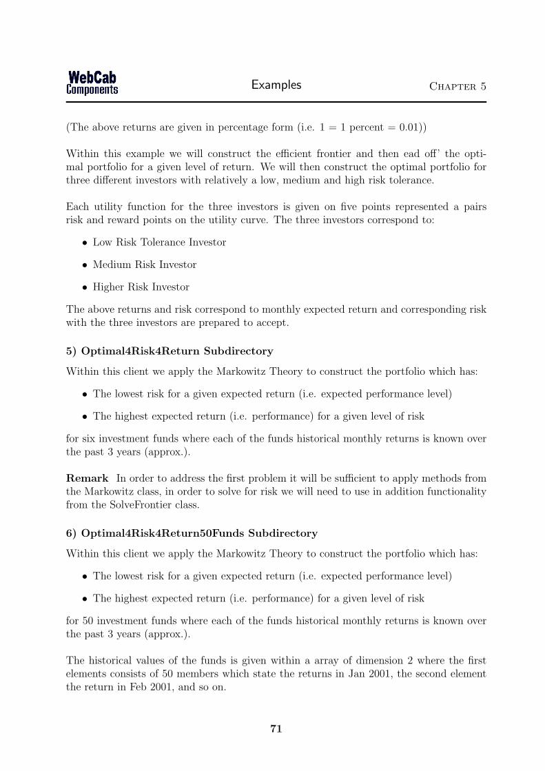
Examples Chapter 5
(The above returns are given in percentage form (i.e. 1 = 1 percent = 0.01))
Within this example we will construct the efficient frontier and then ead off’ the opti-mal portfolio for a given level of return. We will then construct the optimal portfolio forthree different investors with relatively a low, medium and high risk tolerance.
Each utility function for the three investors is given on five points represented a pairsrisk and reward points on the utility curve. The three investors correspond to:
• Low Risk Tolerance Investor
• Medium Risk Investor
• Higher Risk Investor
The above returns and risk correspond to monthly expected return and corresponding riskwith the three investors are prepared to accept.
5) Optimal4Risk4Return Subdirectory
Within this client we apply the Markowitz Theory to construct the portfolio which has:
• The lowest risk for a given expected return (i.e. expected performance level)
• The highest expected return (i.e. performance) for a given level of risk
for six investment funds where each of the funds historical monthly returns is known overthe past 3 years (approx.).
Remark In order to address the first problem it will be sufficient to apply methods fromthe Markowitz class, in order to solve for risk we will need to use in addition functionalityfrom the SolveFrontier class.
6) Optimal4Risk4Return50Funds Subdirectory
Within this client we apply the Markowitz Theory to construct the portfolio which has:
• The lowest risk for a given expected return (i.e. expected performance level)
• The highest expected return (i.e. performance) for a given level of risk
for 50 investment funds where each of the funds historical monthly returns is known overthe past 3 years (approx.).
The historical values of the funds is given within a array of dimension 2 where the firstelements consists of 50 members which state the returns in Jan 2001, the second elementthe return in Feb 2001, and so on.
71

Examples Chapter 5
Remark In order to address the first problem it will be sufficient to apply methodsfrom the Markowitz class, in order to solve for risk we will need to use in addition func-tionality from the SolveFrontier class.
WARNING: This example will take several minutes to run.
7) Optimal4Risk4Return200Funds Subdirectory
Within this client we apply the Markowitz Theory to construct the portfolio which has:
• The lowest risk for a given expected return (i.e. expected performance level)
• The highest expected return (i.e. performance) for a given level of risk
for 200 investment funds where each of the funds historical monthly returns is known overthe past 3 years (approx.).
The historical values of the funds is given within a array of dimension 2 where the firstelements consists of 200 members which state the returns in Jan 2001, the second elementthe return in Feb 2001, and so on.
Remark In order to address the first problem it will be sufficient to apply methodsfrom the Markowitz class, in order to solve for risk we will need to use in addition func-tionality from the SolveFrontier class.
WARNING: This examples will take more than an hour to complete on a desktop ma-chine.
8) EfficientAlternative Subdirectory
Within this example we evaluate using the same historical values as within the examplecontained within the folder ‘Efficient’ and evaluate the portfolio on the Efficient Frontier.The difference between this example and the example contained within the ‘Efficient’ folderin that here we do not use the direction approach of evaluating the portfolio, but use theapproach via the evaluate of the Efficient Frontier at a number of interpolation points.
The rationale for including this examples is to allow the comparison between these two ap-proaches to the evaluation of the optimal portfolio for a given values of the expected return.
Historical Values Used
Within this example we use the following relative historical values of five assets histor-ical returns over the last five periods:
• 1st Asset: 0.03, 0.04, 0.02, 0.05, 0.03
• 2nd Asset: 0.03, 0.040, 0.1, 0.03, 0.035
72

Examples Chapter 5
• 3rd Asset: 0.03, 0.032, 0.033, 0.035, 0.036
• 4th Asset: 0.02, 0.021, 0.021, 0.021, 0.0205
• 5th Asset: 0.02, 0.01, 0.02, 0.015, 0.028
Where the portfolios on the Efficient Frontier can be constructed with respect to thefollowing asset weight constraints:
• 1st Asset Weight Constraints: Lower bound of = 0.05, Upper bound = 0.2
• 2nd Asset Weight Constraints: Lower bound = 0.05, Upper bound = 1
• 3rd Asset Weight Constraints: Lower bound = 0.05, Upper bound = 1
• 4th Asset Weight Constraints: Lower bound = 0.05, Upper bound = 0.5
• 5th Asset Weight Constraints: Lower bound = 0.05, Upper bound = 1
5.2.2 Capital Market Custom Clients
Within this section we describe the custom examples which we provide for the CapitalMarket class. The source code for these examples can be found within sub-directories ofthe directory:
Clients > QAClients > ”Language/Technology” > Portfolio > CapitalMarket
where ”Language/Technology” refers the program language and/or technology (for ex-ample Java, C, Delphi, EJB, COM, Web services, CORBA etc) by which the example arewritten in.
1) CashConstraints Subdirectory
Within this example we illustrate how constraints may be placed onto the levels of thecash held or borrowed to the market by an optimal portfolio constructed in accordancewithin the Capital Asset Pricing Model. We show how the resulting continuous range ofthe values of the expected return and total risk can then be deduced which identify whichoptimal portfolios can be selected when the cash level constraints are observed.
2) Equity Subdirectory
This example illustrates the construction in accordance with the Capital Asset PricingModel (CAPM) of the Optimal Portfolio on the CML where constraints are placed on theasset weights from which the portfolios can be constructed.
This example illustrates the application of the Capital Asset Pricing Model (CAPM) func-tionality implemented within the class CapitalMarket.
73

Examples Chapter 5
In particular, we seek the solution to the following question:
What is the weighting of the Market Portfolio and risk of the optimal portfolios withrespect to the CAPM which can be constructed from 5 assets with historical returns of:
Time interval Asset1 Asset2 Asset3 Asset4 Asset51st interval 500 500 300 200 2502nd interval 450 450 320 210 2703rd interval 500 400 330 215 3004th interval 550 300 350 210 2805th interval 600 350 360 205 290
where the weights of each of the assets of the portfolio constructed must lie between 0.1and 0.5, that is, each asset can have a minimum weights in 10 percent and a maximumweighting of 50 percent with the constructed portfolio.
Question: What if the Market Portfolio’s risk and expected return? In accordance, withrespect to the CAPM what is the optimal portfolios (i.e. lowest risk with a given expectedreturn) which has an expected absolute return of 300 and 210?
Overview of Approach
Once the source data is given we we provide to find the constrained optimal portfoliobe following the below steps:
• Instantiate the Capital Market (main class) and Asset Parameter classes which pro-vide the functionality required.
• Evaluate the covariance and expected returns of the collection of assets from whichthe portfolios can be constructed. This is done using two auxiliary methods from theAsset Parameters class.
• Set the constraints on the asset weights from which the portfolios are constructed.
• We then evaluate the Efficient Frontier on the entire range on which it exists and setits interpolation points to a private field.
• Next we construct the Market Portfolio.
• We then evaluate the risk and expected return of the Market Portfolio which will beused within the follow calculations.
• In order to find the optimal portfolios with respect to the CAPM we evaluate theportfolios of the CML with an expected return of 210 and 300. That is, we evaluatethe weighting of the market portfolio and the risk of each of the portfolios.
74
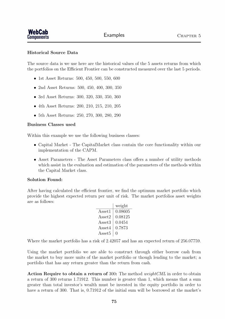
Examples Chapter 5
Historical Source Data
The source data is we use here are the historical values of the 5 assets returns from whichthe portfolios on the Efficient Frontier can be constructed measured over the last 5 periods.
• 1st Asset Returns: 500, 450, 500, 550, 600
• 2nd Asset Returns: 500, 450, 400, 300, 350
• 3rd Asset Returns: 300, 320, 330, 350, 360
• 4th Asset Returns: 200, 210, 215, 210, 205
• 5th Asset Returns: 250, 270, 300, 280, 290
Business Classes used
Within this example we use the following business classes:
• Capital Market - The CapitalMarket class contain the core functionality within ourimplementation of the CAPM.
• Asset Parameters - The Asset Parameters class offers a number of utility methodswhich assist in the evaluation and estimation of the parameters of the methods withinthe Capital Market class.
Solution Found:
After having calculated the efficient frontier, we find the optimum market portfolio whichprovide the highest expected return per unit of risk. The market portfolios asset weightsare as follows:
weightAsset1 0.08605Asset2 0.08125Asset3 0.0454Asset4 0.7873Asset5 0
Where the market portfolio has a risk of 2.42057 and has an expected return of 256.07759.
Using the market portfolio we are able to construct through either borrow cash fromthe market to buy more units of the market portfolio or though lending to the market; aportfolio that has any return greater than the return from cash.
Action Require to obtain a return of 300: The method weightCML in order to obtaina return of 300 returns 1.71912. This number is greater than 1, which means that a sumgreater than total investor’s wealth must be invested in the equity portfolio in order tohave a return of 300. That is, 0.71912 of the initial sum will be borrowed at the market’s
75
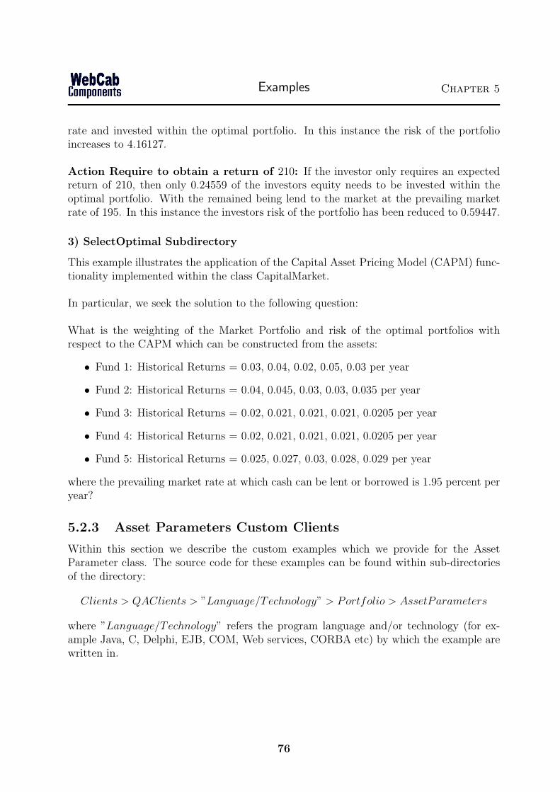
Examples Chapter 5
rate and invested within the optimal portfolio. In this instance the risk of the portfolioincreases to 4.16127.
Action Require to obtain a return of 210: If the investor only requires an expectedreturn of 210, then only 0.24559 of the investors equity needs to be invested within theoptimal portfolio. With the remained being lend to the market at the prevailing marketrate of 195. In this instance the investors risk of the portfolio has been reduced to 0.59447.
3) SelectOptimal Subdirectory
This example illustrates the application of the Capital Asset Pricing Model (CAPM) func-tionality implemented within the class CapitalMarket.
In particular, we seek the solution to the following question:
What is the weighting of the Market Portfolio and risk of the optimal portfolios withrespect to the CAPM which can be constructed from the assets:
• Fund 1: Historical Returns = 0.03, 0.04, 0.02, 0.05, 0.03 per year
• Fund 2: Historical Returns = 0.04, 0.045, 0.03, 0.03, 0.035 per year
• Fund 3: Historical Returns = 0.02, 0.021, 0.021, 0.021, 0.0205 per year
• Fund 4: Historical Returns = 0.02, 0.021, 0.021, 0.021, 0.0205 per year
• Fund 5: Historical Returns = 0.025, 0.027, 0.03, 0.028, 0.029 per year
where the prevailing market rate at which cash can be lent or borrowed is 1.95 percent peryear?
5.2.3 Asset Parameters Custom Clients
Within this section we describe the custom examples which we provide for the AssetParameter class. The source code for these examples can be found within sub-directoriesof the directory:
Clients > QAClients > ”Language/Technology” > Portfolio > AssetParameters
where ”Language/Technology” refers the program language and/or technology (for ex-ample Java, C, Delphi, EJB, COM, Web services, CORBA etc) by which the example arewritten in.
76

Examples Chapter 5
1) ForwardLooking Sub-directory
Suppose you have the following data regarding 3 securities.
State 1st Asset 2nd Asset 3rd Asset Probability1st state 100 120 200 0.12nd state 120 130 150 0.73rd state 130 140 140 0.2
Each cell in this table contains two values: the return of the asset in one of three states,and the probability of that state occurring.
In our example we evaluate the following:
• The expected variance of each asset:
– for the 1st asset var = 60
– for the 2nd asset var = 29
– for the 3rd asset var = 261
• The expected return for each asset:
– for the 1st asset exp = 120
– for the 2nd asset exp = 131
– for the 3rd asset exp = 153
• The covariance between the 1st and 2nd Asset is: 40
Remark Since the returns of the assets are given as absolute valuee of the expected returnsevaluate will also be given in absolute values rather than in relative (i.e. percentage) terms.
Portfolio constructed with Equal Weighting between the three assets avail-able
Suppose that you have a portfolio containing equal shares from each of the three As-sets available. That is, the weighting of each of 1st, 2nd and 3rd asset is 1/3. For thisconstructed portfolio we evaluate the following properties:
• The expected return which is evaluated to be: 134.66667
• The portfolio’s risk which is evaluated to be: 2.21108
• The variance of returns which is evaluated to be: 4.88889
77
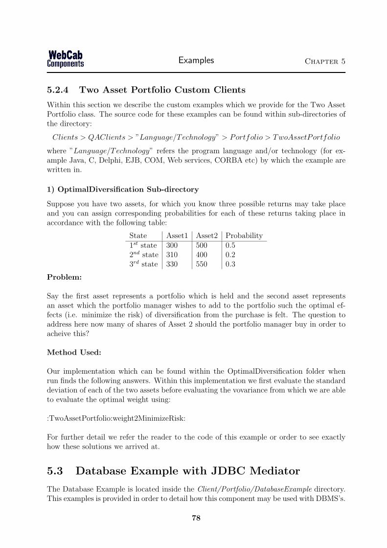
Examples Chapter 5
5.2.4 Two Asset Portfolio Custom Clients
Within this section we describe the custom examples which we provide for the Two AssetPortfolio class. The source code for these examples can be found within sub-directories ofthe directory:
Clients > QAClients > ”Language/Technology” > Portfolio > TwoAssetPortfolio
where ”Language/Technology” refers the program language and/or technology (for ex-ample Java, C, Delphi, EJB, COM, Web services, CORBA etc) by which the example arewritten in.
1) OptimalDiversification Sub-directory
Suppose you have two assets, for which you know three possible returns may take placeand you can assign corresponding probabilities for each of these returns taking place inaccordance with the following table:
State Asset1 Asset2 Probability1st state 300 500 0.52nd state 310 400 0.23rd state 330 550 0.3
Problem:
Say the first asset represents a portfolio which is held and the second asset representsan asset which the portfolio manager wishes to add to the portfolio such the optimal ef-fects (i.e. minimize the risk) of diversification from the purchase is felt. The question toaddress here now many of shares of Asset 2 should the portfolio manager buy in order toacheive this?
Method Used:
Our implementation which can be found within the OptimalDiversification folder whenrun finds the following answers. Within this implementation we first evaluate the standarddeviation of each of the two assets before evaluating the vovariance from which we are ableto evaluate the optimal weight using:
:TwoAssetPortfolio:weight2MinimizeRisk:
For further detail we refer the reader to the code of this example or order to see exactlyhow these solutions we arrived at.
5.3 Database Example with JDBC Mediator
The Database Example is located inside the Client/Portfolio/DatabaseExample directory.This examples is provided in order to detail how this component may be used with DBMS’s.
78

Examples Chapter 5
Before being able to run this examples you will need to complete the following steps:
1. Installing our Tables (MySQL Only)In order to create the database structure from which you are able to load the outputresults, you will need to run the ‘create.sql’ scripts in the ‘Data’ subdirectory. Openthe MySQL prompt from the ‘Data’ subdirectory and:
• Select (or create and then select) a database you can spare for a table namedHISTORICAL RETURNS. For example, if you have decided using the ‘test’database, you would optinally type the SQL command to create it (unless italready exists):
CREATE DATABASE test;
and then, you would type the following to select it:
USE DATABASE
• Run the ‘create.sql’ SQL script located in the ‘Data’ subdirectory of the currentdirectory by typing at the same MySQL prompt the following:
source create.sql
If this fails, make sure you have started the MySQL prompt from the ‘Data’subdirectory (this is where the database files for this example are stored).
2. Configuring the Database ConnectionEdit the Java source code file by filling out JDBC information about your database,such as:
(a) Driver Name (e.g. com.jdbc.mysql.Driver)
(b) JDBC Url (e.g. jdbc:mysql://localhost/test)
(c) Username and Password
If you are unsure whether you have a JDBC Driver for your Database, skip this stepand try running the example with the predefined values. If that fails, you will needto probably download the latest driver.
3. Running the example
Run the ‘compile’ script (compile.sh for Linux, compile.bat for Windows) to compilethe Java source code, and then the ‘run’ script to see the results.
Uninstalling the Source Data
To delete all the tables used in this example, open the MySQL prompt from the ‘Data’subdirectory, select the database where you created the tables, and run the following:
source delete.sql
79
Examples Chapter 5
5.4 How to use Markowitz Theory?
Within this section we provide several step-by-step guides on how to perform many ofthe most required tasks when apply Markowitz Theory. The methods references withinthis section will correspond to methods of the same name found within the Markowitz,AssetParameters or PerformanceEvaluation class’s.
5.4.1 How to find the portfolio from a collection of assets thatexhibit the lowest risk for a given expected future return?
The problem of finding the optimal portfolio with the lowest risk with a given expectedreturn from a collection of assets of which the historical performance is known, involvesapplying two methods, namely:
• calculateEfficientFrontier - we construct the efficient frontier that consists of a con-tinuously varying family of portfolios
• efficientFrontier - this method selects a portfolio determined by its expected returnfrom the family of portfolios on the efficient frontier
Constructing such a portfolio is the main application of classical Markowitz Theory. Thatis, if you take a collection of assets historical performance from which you imply expectedperformance. By evaluating the covariance matrix of the assets (see section entitled, Howto evaluate the covariance matrix?”) and the efficient frontier (see section entitled, Howto construct the Efficient Frontier?”), you may evaluate the optimal risk by applying themethod:
efficientFrontier(double expectedReturn, int numberOfAssets)
from the Markowitz component.
Remark When we refer to the optimal risk we mean the minimal risk for a given ex-pected return which is the same thing as saying the portfolio which is expected to exhibitthe smallest standard deviation of its value for a given level of expected return.
5.4.2 How to construct the Efficient Frontier?
The Efficient Frontier is constructed by applying the following Markowitz class method:
public void calculateEfficientFrontier(double minimumExpectedReturn,
double maximumExpectedReturn,
double[][] covarianceMatrix,
double[] expectedReturns,
int numberInterpolationPoints,
double precision)
80

Examples Chapter 5
The developer will need to provide the correct input parameters starting with the fol-lowing two:
double minimumExpectedReturndouble maximumExpectedReturn
The minimum and maximum expected returns can be taken to be the minimum andmaximum historical returns from the best performing and worst performing assets withinthe given collection which we will use to construct the optimal portfolio. Since these twoextremes certainly suffice (i.e. allow all potential optimal portfolio’s to be considered), andin the general case these extreme values may even themselves represent optimal portfolios,which in fact only be the case if the covariance matrix is the Identity matrix.
double[][] covarianceMatrix
We apply the method ‘covarianceMatrix’ within the AssetParameters class to the databasetable that contains the assets historical values from which the portfolio will be constructed.The historical data we are provided with should be stored within a database table in orderto apply this method directly.
double[] expectedReturns
Please see the section entitled ”How to estimate the expected return for the historicalreturns?”
int numberInterpolationPoints, double precision
The input value’s for these parameters is just a matter of balancing speed and accuracy.
Remark The Markowitz class uses highly optimized algorithms to construct the Effi-cient Frontier that leads to the construction of the optimal risk-return portfolio. Thisallows the optimal Portfolio to be constructed in one or two minutes for 100+ assets usinga commodity desktop PC. Saving the end user time and offering the convenience of beingable to use a desktop PC equipment rather than specialist server hardware.
5.4.3 How to estimate the expected return from the historicalreturns?
Say your source data is the ‘historical’ monthly performance of a given fund. If we assumethat the historical returns of this fund will be closely related to the future expected returns.
81

Examples Chapter 5
Then we will be able to estimate the future expected returns using the method:
expectedReturn(double[])
from the AssetParameters class.
Further Discussion
Here as in all estimates of the fluctuation of the price (or risk) there will always be twotypes of risk related to the application of the model. Namely the market risk itself and therisk that the market risk (or structure) will change. The success of any model will dependon its ability to adapt to changes in the market dynamics.
Towards this end we offer a number of approaches to estimating the expected returnedwhich one could use for a variety of differing market dynamics. These procedures arecontained within the AssetParameter class and include:
• Arithmetic Historical average - Take the historical return over a given period and takethe expected future return to be the arithmetic average of the historical values. Saywe take the last 6 monthly historical returns, then the probability of the market stateswhich deliver each of these 6 historically recorded returns over the last 6 months is16.
• ARCH Type Model - This is an averaging procedure which attaches more weight tomore recently measured values. For example, we could take:
expectedReturn =∑
(exp(−i)historicalReturn[i])
Say we take the last 6 monthly value again in order to estimate the expected futurereturn. The probability of the market states that delivered each of the return foundin the last six months is:
exp(−i)∑i exp(i)
for i = 0, . . . , 6.
Our implementation of the ARCH model assumes that the underlying asset hasa drift in accordance to the characteristic line. Under this assumption the ARCHmodel provides an effective model for assets, which depend linearly on stocks or stockindexes.
Remark Predictive models of ARCH/GARCH type or models involving technical orfundamental analysis are not prescriptive and hence will depend heavily on the choices ofthe parameters the user makes. Saying this, these models enable the user to ensure thatwhatever the variables used the resulting model will exhibit certain qualitative propertieswhich are embodied within the model itself.
82
Examples Chapter 5
5.4.4 How can I measure the performance characteristics of aportfolio?
One of the core principles of ‘Markowitz Theory’ (and CAPM), is that investors will onlyaccept higher risk for a higher expected return. Therefore, since we are working withinthis framework it is only natural to consider the risk adjusted performance of a portfolioand related methods thereof. Within this product we have including methods by whichthe risk adjusted and non-risk adjusted return can be evaluated.
Risk Adjusted Performance
In order to evaluate the risk adjusted return we use methods from the PerformanceEvalu-ation class. In particular, we use one of the following two methods:
• Sharpes Ratio - This performance measurement parameter is the most widely used.The higher the value the better the portfolios risk return profile is said to be. Toevaluate Sharpes Ratio use the method SharpesRatio.
• Treynors Ratio - This measure takes into account the systematic risk (or beta) andthe average return when assessing the overall risk adjusted return of the portfolio.To evaluate Treynor’s performance measure use the method treynorsMeasure.
Non-risk adjusted Performance
The non-risk adjusted performance of a portfolio can be evaluated by using the methodsTotal Return and Portfolio Return within the performance evaluation class. The Portfo-lio Return method evaluates the arithmetic return of the portfolio over a period of timewhere the return of each asset over the period and its initial portfolio weight is known.The total return method allows you to evaluate the return form the portfolio when cashdisbursements or dividends are taken into account.
Even though these measures are not risk adjusted the user can still use then in injunctionwith a measure of the risk of the portfolio in order to get a better feel for a portfoliosoverall characteristics. The risk of a portfolio, can be evaluated by the method:
portfolioRisk(double[] weight, double[][] covarianceMatrix)
which is contained within the portfolio class.
83

Chapter 6
Guide to WebCab Components
6.1 The Company
WebCab is a privately owned British company that has built business solutions since itsinception in 1999. We continue to refine and develop our Mathematical and FinancialFramework which we have implemented within the J2SE, J2EE and .NET platforms.
6.2 Presentation of Products
We aim to provide good quality, useful information to help you decide which J2SE Com-ponent best suits your development needs. WebCab is committed to honesty and realismwhen presenting our products. In order to achieve this a detailed, clear and factual stylefor presentation is adopted within our documentation and marketing material.
6.3 Supported Clients, IDEs, Containers and DBMSs
We support all major development, server and client side technologies. Each product con-tains detailed examples and advice concerning the integration of our components withinexisting infrastructure. Our documentation provides the information that the developerneeds to get their applications up and running as quickly and as easily as possible.
We detail exactly how the developer can use our J2SE Components with the followingtechnologies:
• Client containers - Internet Explorer, Netscape Navigator, Mozilla, Opera
• IDEs - JBuilder, BEA Studio, Sun ONE (formerly Forte For Java), Eclipse, OracleJDeveloper
• Client Side Technologies - Application Clients, Frames, Applets
• DBMS - Oracle, IBM DB2, SQL Server, Sybase, MySQL
84
Guide to WebCab Components Chapter 6
• Platforms - Windows XP/2000/NT, Linux, Solaris, IBM AIX, HP-UX
For these technologies we include all the installation scripts and template examples whichwill help the developer quickly and easily assemble their multi-tier enterprise application.
6.4 Transparent Functionality
All technical and business intelligence incorporated within our products is described withinthe associated documentation. This allows the developer to see the nature of the method-ology implemented within our proprietary algorithms.
6.5 Code Conventions
WebCab adheres to the ‘Code Conventions for the Java Programming Language’ as spec-ified on April 20, 1999 by Sun Microsystems Inc. These conventions cover filenames, fileorganization, indentation, comments, declarations, statements, white space, naming con-ventions and programming practices. Code conventions improve the readability of thesoftware, allowing engineers to understand new code more quickly and thoroughly.
6.6 Company Culture and Activity
WebCab Components is focused solely on the production of high quality software moduleswithin our Mathematical and Financial Framework. The WebCab team contains a widerange of expertise and experience within the academic, investment banking and softwaredevelopment worlds.
Within the company there exists significant internal competitive pressures with constantpeer review and evaluation, resulting in higher quality products, which adhere to highprofessional standards and offer extended functionality.
6.7 Product Life cycle
We continuously add value to our products by evolving them according to new J2SE spec-ifications, customer feedback and market demands. We give particular emphasis to incor-porating our clients suggested modifications and additions into our product developmentcycle.
6.8 Support, Warranty and Upgrades
WebCab warrants that each component will perform substantially in accordance with theaccompanying written material. We provide with all our products without charge sixty
85
Guide to WebCab Components Chapter 6
(60) days product support services including fixing bugs, compatibility issues and othertechnical support issues.
All maintenance updates (including service packs) will be distributed free of additionallicense cost. New version releases of this product will be offered to present licensee holdersat a greatly reduced rate.
Dr Ben Fairfax
Founder and CEO
WebCab Components - From Developer, To Developer
Java and all Java-based marks are trademarks or registered trademarks of Sun Microsystems, Inc. in
the U.S. and other countries.
86


![i.uran.rui.uran.ru/webcab/system/files/journalspdf/journal... · A Promising Ionic Liquid [BMIMl[FeC14] for the Extractive Separation of Aromatic and Aliphatic Hydrocarbons Salem](https://img.pdfslide.us/doc/110x75/5eb72f46dc05b955910a61c7/iuranruiuranruwebcabsystemfilesjournalspdfjournal-a-promising-ionic.jpg)