€¦ · Web viewSome important consequences of anthropic changes in land use and land cover in South America have ... 2012; The World Bank ... on wheat, rice and corn crops

CLIMATE CHANGE AND AGRICULTURE: DO ECOSYSTEM SERVICES MATTER?

Bruno César Brito Miyamoto1a, Alexandre Gori Maia1b, Junior Ruiz Garcia2c

1Center for Agricultural and Environmental Economics, University of Campinas, Brazil 2Department of Economics, Federal University of Parana, Brazil

aE-mail: [email protected] bE-mail: [email protected]

cE-mail: [email protected]

Área 11 - Economia Agrícola e do Meio Ambiente

JEL: C23,Q51,Q57

Abstract

Climate change is expected to cause several impacts on agriculture. Nonetheless, adaptive strategies such as access to irrigation and environmentally sustainable techniques may affect the ability to cope with these impacts. We analyze how agricultural technologies and environmental preservation have attenuated the impacts of extreme climate events on agricultural production. Analyses are based on a panel with information for 568 municipalities in the state of São Paulo (Brazil) between 1990-2014. We first use multivariate statistical analysis to define six groups of localities according to their levels of agricultural development and land cover. Secondly, based on fixed effect estimates, we analyze the relationship between the dynamics of extreme climate events and agricultural production in each group of localities. Results highlight that both technological and environmental factors contribute to increases in agricultural productivity. More importantly, agriculture practiced with high levels of environmental preservation tends to be more resilient to extreme temperature and precipitation events.Keywords: extreme events, agricultural production, environmental sustainability, production practices

Resumo

Espera-se que as mudanças climáticas causem vários impactos na agricultura. No entanto, estratégias adaptativas, como o acesso à irrigação e técnicas ambientalmente sustentáveis, podem afetar a capacidade de lidar com esses impactos. Analisamos como as tecnologias agrícolas e a preservação ambiental atenuaram os impactos de eventos climáticos extremos na produção agrícola. As análises são baseadas em um painel com informações para 568 municípios do estado de São Paulo (Brasil) entre 1990-2014. Utilizamos primeiro análises estatísticas multivariadas para definir seis grupos de localidades de acordo com os seus níveis de desenvolvimento agrícola e tipos de cobertura. Em segundo lugar, com base em estimativas de efeitos fixos, analisamos a relação entre a dinâmica de eventos climáticos extremos e a produção agrícola em cada grupo de localidades. Os resultados destacam que tanto fatores tecnológicos como ambientais contribuem para o aumento da produtividade agrícola. Mais importante ainda, a agricultura praticada com altos níveis de preservação ambiental tende a ser mais resiliente a temperaturas extremas e aos eventos de precipitação.Palavras-chave: eventos extremos, produção agrícola, sustentabilidade ambiental, práticas de produção.

1

mailto:[email protected]



1. IntroductionClimate change is expected to cause several impacts on agriculture, primarily through increases in average temperature and in the intensity and frequency of extreme events, such as heavy precipitation and prolonged droughts (IPCC 2014). Studies have highlighted how less developed regions and more vulnerable farmers tend to be specially affected by climate change, since they lack the basic social and economic capital needed for adaptive strategies, such as access to irrigation and drought-tolerant crops (Wreford, Moran, and Adger 2010; Mendelsohn and Dinar 2009). South American countries, for example, are already suffering significant changes in average rainfall and temperature, increases in the occurrence of warmer nights in tropical regions, and dry spells in semiarid regions (Vergara 2009; PBMC 2014; Marengo et al. 2010). The patterns of land use and the provision of ecosystem services are also expected to affect the ability to cope with climate change. Although humans have appropriated an increasing share of the planet’s resources, changes in land use and land cover have potentially undermined the capacity of ecosystems to sustain food production, maintain freshwater and forest resources, regulate climate and air quality, and ameliorate infectious diseases (Foley et al. 2005). Some important consequences of anthropic changes in land use and land cover in South America have been hydric degradation, loss of soil fertility, erosion, and desertification (Marengo et al. 2012; The World Bank 2012). We analyze how agricultural technologies and environmental preservation practices may attenuate the impacts of extreme climate events on agricultural production in the state of São Paulo, Brazil. Firstly, we use multivariate statistical analysis to define six groups of MCAs according to their levels of agricultural development and land cover. Secondly, based on a panel with 568 Minimum Comparable Areas (MCAs, which are groups of historically comparable municipalities) between 1990 and 2014, we use fixed effect estimates to analyze the relationship between the dynamics of climatic variables and agricultural production in each group of MCAs. We analyze the impacts on the (i) total value of production and (ii) the log of the physical production of sugarcane and orange, the main agricultural activities in the region. São Paulo is the most developed state, and the state with the second largest value of agricultural production in the country. Although agriculture represents only 2% of the state’s GDP, the activity is important for local and regional economies because industrial and high-paying services employment are concentrated in a few metropolitan areas. Furthermore, São Paulo’s agricultural sector plays an important role in Brazilian agribusiness, since the state is the leading national producer of sugarcane/ethanol, sugarcane/sugar and orange juice. In 2013, the state of São Paulo possessed the highest gross value of agricultural production among Brazilian states. Currently, São Paulo ranks second in the national ranking, only behind the state of Mato Grosso, the largest producer of soybeans and cotton in Brazil. The cultivation of the main agricultural product in the state, sugarcane, is based on rainfed irrigation, making it more dependent on environmental and climate conditions, especially rain patterns. Despite the fact that São Paulo is located in a region with high levels of precipitation and a rich supply of fresh water, it has experienced critical moments of water shortage in recent years as a result of both growth in demand and the reduction in regular supply of water resources. Observers have identified climate change as one of the main factors responsible for the extremely low levels of precipitation observed in the early 2010s.

2. Literature Review

The changes in land use and land cover are affecting the ecosystem dynamic (IPCC, 2014; World Bank, 2012; PBMC, 2013). Many regions are suffering with the hydric degradation, fast changes in climate, loss of soil fertility, erosion, desertification, and so on (Marengo, 2007a; Marengo et al., 2011). The IPCC is the global main research’s institution assessing of the potential impacts of climate change (IPCC, 2014). In Brazil, the National Institute for Space Research (INPE) projected an increase in average temperature by

2

2100 from 4° C to 6° C in pessimistic scenario, or from 1° C to 3° C in optimistic scenario (Marengo 2007a; PBMC, 2013).According to IPCC (2007a; 2007b), Marengo (2007a; 2007b) and PBMC (2013), the main impacts rising of average temperature may be: advance arid and semiarid areas; desertification; loss of biodiversity; decrease agricultural production and productivity; changes in rainfall; and other effects. In Brazil, INPE’s projections indicate decrease in rainfall in the North region and rise in droughts in the Northeast (Marengo 2007b; PBMC, 2013).The Brazilian agriculture can be strongly affected by climate change (Monteiro, 2011). Estimate realized by Monteiro (2011) indicate that the rising of the global average temperature can reduce the area for soybean, coffee, corn, rice, and other crops. These impacts can result in loss of the R$ 7.5 billion by 2020 to Brazilian agriculture. Other estimate was realized by Moraes (2010), where the loss to Brazilian agriculture can reach 0.29% of the GDP (Gross Domestic Product) based on A2/2020 scenario, or 1.09% of the GDP in B2/2070 scenario. Besides, IPCC’s report (2014) indicate clear impacts on wheat, rice and corn crops.Changes in the frequency and intensity of extreme weather events at the local level are also expected with the long-term transformations that will be imposed by global climate change. Extreme precipitation events such as droughts and floods tend to represent more and more sources of agricultural losses due both to direct and indirect effects of changes in soil moisture conditions (Rosenzwieg et al., 2001).Severe droughts can contribute to the elevation of plant temperature, due to the closure of the stomata and the reduction of transpiration, and to the increase of pests and diseases due to the reduction of the population size of natural enemies (Rosenzwieg et al., 2001; Van Der Velde, 2012). Prolonged droughts also increase the risk of soil erosion by winds, and when followed by heavy rains, increase the potential for flooding due to reduced soil water absorption capacity, which creates favorable conditions for fungal infestation in leaves and roots (Rosenberg et al., 2001, Várallyay, 2010, Knapp et al., 2008).In addition to physically damaging the plants, high levels of precipitation, storms and floods can generate productive losses in agriculture by delaying planting and harvesting operations (Van Der Velde, 2012). Excessive precipitation can also cause long-term adverse effects such as leaching and erosion, if there is no conservation-oriented soil management (Vallesley, 2010; Deelstra et al., 2011; Jorgensen & Termansen, 2015).Soil water storage capacity is one of the factors that determine how ecosystems will respond to future changes in precipitation regimes. Soil water storage depends on soil and subsurface soil conditions, as well as vegetation characteristics, such as type, density, species composition and root characteristics (Várallyay, 2010). Ecosystems where there is a predominance of deep roots may present greater resilience to water fluctuations in the soil (Knapp et al., 2008, Nepstad 1994, Kustura et al. 2007) The role of biological diversity in the stability of ecosystems due to environmental fluctuations is an object of intense debate in ecological research. One of the most important themes linked to this debate is "insurance hypothesis"(Yachi e Loreau, 1999; Naeem & Li, 1997; Mariotte et al., 2013). According to "insurance hypothesis" the diversity of species in an ecosystem increases the chance that ecosystem functions will remain stable in the face of an environmental disturbance or extreme climatic event (Mariotte et al., 2015). An ecosystem with greater diversity would be more likely to have a species capable of replacing one less adapted to the new environmental condition imposed and thus guarantee the stability of a given ecosystem service (Borrval & Ebenman, 2008).

3. Data and Methods

3

3.1. Clusters of land cover

Based on the maps of land cover provided by the Brazilian Institute of Geography and Statistics (IBGE), we identified eight classes of land cover in São Paulo: agriculture; urban areas; water and humid forests; mosaic of agriculture and remaining forests (agriculture/forests); mosaic of natural vegetation, forests and agriculture (forest/agriculture); pastures; silviculture; and forests. This information was available for the years 2000, 2010, 2012 and 2014 (Table 1). The main change observed in this period was the shift from forests (declining from 10.7% of the total in 2000 to 9.1% in 2014) and pasture (declining from 12.1% to 10.8%) to agricultural areas (increasing from 26.5% to 31.4%), mainly sugarcane.

Table 1 – Percentage of the total area according to land cover type, São Paulo

Land CoverYear

2000 2010 2012 2014Agriculture 26.5 27.5 29.1 31.4Urban 3.3 3.3 3.3 3.3Water 3.5 3.5 3.5 3.5Agriculture/forest 33.8 33.6 32.7 32.5Forest/agriculture 6.5 6.2 6.0 5.7Pasture 12.1 12.3 12.6 10.8Silviculture 3.6 3.9 3.5 3.8Forest 10.7 9.7 9.3 9.1

Source: Elaborated by the authors using data from the IBGE

We then computed the average percentage value of each MCA’s total area covered by each one of the eight classes in the whole period. The classification of municipal observations in clusters of land cover was defined by the technique of cluster analysis. Cluster analysis defines hierarchical groups of observations within a data set. There are several methods that may be employed in this process, but all are based on the same principle of hierarchical clustering. Initially, each observation is considered as a cluster. The two closest clusters are then joined to form a new cluster, and so on until the method forms a maximum number of clusters predetermined by the researcher. The difference between alternative clustering methods is basically the way in which the distance (or dissimilarity) between clusters is calculated.

The clustering method employed in this study is the Ward method, an aggregation strategy based on the analysis of variance within and between the groups formed. The aim of this method is to create hierarchical groups in such a way that the variance within groups is minimal and the variance between groups is maximal (Crivisqui 1999). The aggregation criterion consists of finding the next group that minimizes the variability within the newly-formed group. To facilitate the understanding of the variability within groups, they are usually divided by the total variance to represent a ratio of the maximum achieved variability (semipartial R2).

3.2. Factors of production practices in agriculture

Variables relating to production practices in agriculture were obtained from the Survey of Agricultural Production Units from 2007/2008 (LUPA, Levantamento Censitário de Unidades de Produção Agrícola), provided by the Institute of Agricultural Economics (IEA, Instituto de Economia Agrícola). These variables refer to ratios between the number of units of technological systems or techniques per farm (Table 2): irrigation systems, sowing machines, plowing machines; tractors; other machines; and adoption of soil treatment.

4

Table 2 – Ratio between number of units of technological systems or techniques and farms, São Paulo

Technique units / farm

Irrigation 0.082Sowing machine 0.076Plowing machine 0.259Tractor 0.484Other machines 0.123Soil treatment 0.954

Source: Elaborated by the authors using data from the LUPA

Next, factor analysis was applied to identify a common factor of production practices that was strongly and positively correlated with these variables. The method assumes that observable variables related to production practices can be expressed by linear combinations of unobservable and uncorrelated factors (Kim and Mueller 1978). These factors are also called common factors, since they contribute to explain the variability of the group of observable variables. In the factor analysis, commonality represents the share of the total variability of the i-th observable variable explained by the common factor. The total variability explained by each common factor represents the discriminatory power of the respective factor over all observable variables. It is also typically expressed in relative terms, i.e., as a percentage of the total variability of the observed variables. In turn, the factor loadings are used to interpret the factors’ meaning, considering their linear relation and their relevance in predicting each observable variable. To obtain the common factor, we use principal-component factor analysis due to its operational simplicity and the analytical consistency of its results in our case. This technique provides the factor that contributes most to explaining the variability of observable variables. Since the common factor has an average value of 0 (and standard deviation equal to 1), we divide the MCAs into two groups of production practices: (i) positive factor scores were classified into a high-technology group; and (ii) those with negative factor scores were classified into a low-technology group.

3.3. Climate variables

Climate variables for the MCAs were obtained by interpolating point data from conventional weather stations of the National Meteorological Institute (INMET). Daily data on temperature and precipitation were interpolated for all MCAs located in the State of São Paulo. The interpolation was performed by the Inverse Distance Weighted method, which is based on the weighted linear combination of the data collected in each meteorological station, using the inverse of the distance as a weighting factor (Amorin et al. 2011). After interpolation, we computed the average values of temperature and precipitation for each MCA and for each season: spring, summer, autumn and winter (Figure 1). The most striking changes were the decline in precipitation during summer and spring in the 2010’s, and the overall trend of rising temperature in the winter.

5

Figure 1 – Average values of temperature (oC) and precipitation (mm/day) by season, São PauloTemperature Precipitation

Source: Elaborated by the authors using data from INMET

Extreme temperature and precipitation events were controlled for by 16 dummy variables identifying the seasons of the year t (p, for spring, s for summer, a for autumn and w for winter) with average temperature (Tkt, where k=p, s, a or w) and total precipitation (Pkt) lower or higher than a historical threshold. Historical

thresholds are defined by one standard deviation (σ T k for temperature and

σ Pk for precipitation) from the average value (T k or Pk ) in season k. In other words, we have for temperature:

T k +=¿¿ and T k−¿¿¿

And for precipitation we have:

Pk +=¿¿ and Pk−¿¿¿

3.4. Production model

Information on agricultural production was obtained from the Brazilian Institute of Geography and Statistics (IBGE), and refers to the Municipal Agricultural Survey (PAM, Pesquisa Agrícola Municipal). We analyze the total value of production in each MCA (in constant values) and the total physical production (in tons) of the two main crops in the state: sugarcane (58% of the total value) and oranges (10% of the total value).

The relationship between the dynamics of climate variables and agricultural production in each group was analyzed by panel data models. The dependent variables Y are (i) the log of total value of production and (ii) the log of the physical production of sugarcane and orange. The explanatory variables are the binary climate

variables defined in topic 2.3 (T k+ , T k− , Pk+ and Pk− ) and the total harvested area A of each crop. In the case of the total value of production, Ai represents the total harvested area in each MCA i. Unobserved regional (ri) and temporal (ct) factors are controlled by fixed effects. This relationship is given by:

6

Y it=α+δAit+ ∑k=p , s ,a , w

βk(T k it+)+ ∑

k=p , s ,a , wθk (T k it

−)+ ∑k=p , s , a ,w

φk (Pk it+)+ ∑

k=p , s ,a , wϕk ( Pkit

−)+ri +c t +εit(1)

The coefficients of interest are β , θ , φ ϕ , which represent the impact of extreme events on agricultural production Y, after controlling for area (A) and unobserved regional (r) and temporal effects (c). We adjust equation (1) for each group of MCAs, which were defined by the combination of the clusters of land cover (defined in 2.1) and the groups of production practices (defined in 2.2). The idea is to analyzed to what extent differing levels of environmental preservation and production techniques can mitigate the impacts of extreme events on agricultural production.

Since we do not have historical values for the levels of environmental preservation and production techniques across the whole period, we assume that changes observed in time (ct) are independent of differences between MCAs (ri). This may not be totally true, given that the dynamics of agricultural advances and land cover may have been more pronounced in some specific regions. In other words, some MCAs may shift between groups of land cover and/or production practices in the period of analysis. Nonetheless, we believe that the period 1990-2014 is short enough to consider that differences between regions are constant over time. Later versions of this study would consider the interaction between ri and ct.

4. Results

4.1. Groups of land cover and production practices

The cluster analysis was applied to identify groups of MCAs with relatively homogeneous percentages of land cover. We selected three clusters, and the differences between the mean values of these clusters accounted for 51% of the total variability (semipartial R2) observed between the annual values of MCAs. The average characteristics of the three clusters are presented in Table 3.

The first cluster (agriculture) contains 145 MCAs (26% of the total) and represents predominantly agricultural areas. The largest share of land is covered exclusively by agriculture (70.5%) and by mosaics of agriculture and remaining areas of forest (13.5%). Only 2% of the area is covered by forest or by areas of forest integrated with small areas of agriculture.

Cluster two (agriculture/forest), the largest group with 243 MCAs (43% of the total), represents agricultural areas with a larger level of environmental preservation. It is predominantly covered by mosaics of agriculture and forest (59.6%) and by agriculture alone (18.9%). In comparison with the first cluster (agriculture), this second group also highlights a larger share of areas covered by forest integrated to agriculture (6.5% compared to 1.6%), silviculture (3.3% compared to 1.5%) and forest (1% compared to 0.4%).

Table 3 – Proportion of each land cover type according to clusters of MCAs, São Paulo

VariableGroup of land cover

Agriculture Agriculture / forest

Urban / Pasture Total

N 145 243 180 568

Agriculture 0.705 0.189 0.079 0.286Urban 0.045 0.028 0.103 0.056Water 0.025 0.030 0.034 0.030Agriculture/forest 0.135 0.596 0.226 0.361Forest/agriculture 0.016 0.065 0.089 0.060

7

Pasture 0.055 0.050 0.252 0.115Silviculture 0.015 0.033 0.008 0.020Forest 0.004 0.010 0.208 0.071

Source: Elaborated by the authors using data from IBGE

The third cluster, urban/pasture, represented by 180 MCAs (32% of the total), is predominantly urban (10% of the area). Areas covered exclusively by agriculture or by the integration between agriculture and forests represent only 39.4% of the territory, as opposed to 85% in the first two clusters. This cluster is also characterized by the dichotomy between pastures (25.2%) and forest (20.8%).

Next, each cluster of land cover was disaggregated into two groups: low and high technology. The technology groups were defined using scores obtained by factor analysis (topic 2.2). We selected the first common factor, which represented 46.1% of the total variability of the six observed variables of production techniques (irrigation systems, sowing machines, plowing machines, tractors, other machines, and adoption of soil treatment). All observed variables presented positive correlations with the selected common factor, with coefficients ranging from 0.40 (irrigation) to 0.87 (tractor). The correlations (factor patterns) and the standardized scoring coefficients of each variable with the common factor are presented in Appendix A. The MCAs with positive factor scores were classified into a high-technology group, while those with negative factor scores were classified into a low-technology group..

Table 4 characterizes the groups of land cover and production techniques. The use of production techniques differs sharply between the high and low technology groups. For example, within the group of urban/pasture land cover, the use of irrigation systems is almost six times higher in the high-technology group (31.8 / 100 farms) than in the low-technology group (5.4 / 100 farms). Differences in the use of irrigation systems are also notable within the high-technology groups. The use of irrigation is more pronounced in the group of urban/pasture land cover (31.8 /100 farms), and rare in the group of agriculture land cover (6.8 / 100 farms). These differences may reflect both the type of crop and environmental needs.

Table 4 - Ratio between the number of technological systems or techniques per farm according to groups of land cover and production techniques (High and Low), São Paulo

Production Technique

Agriculture Agriculture / Forest Urban / Pasture

High Low High Low High LowN 91 54 107 136 43 137

Irrigation system 0.068 0.022 0.115 0.040 0.318 0.054Sowing machine 0.158 0.048 0.107 0.040 0.095 0.033Plowing machine 0.396 0.167 0.379 0.175 0.359 0.148Tractor 0.794 0.323 0.682 0.310 0.729 0.255Other machines 0.271 0.072 0.172 0.061 0.148 0.053Soil treatment 1.133 0.881 1.200 0.789 1.157 0.748

Source: Elaborated by the authors using data from LUPA

Table 5 presents the average values over the entire period of analysis (1990-2014) for the agricultural production of each group of land cover and production techniques. The groups agriculture and agriculture/forest concentrate roughly 90% of the total value of production, as well as more than 90% of the

8

total production of sugarcane and oranges. In these two groups of land cover, a higher rate of use of production techniques has a positive effect on the sugarcane yield, where the production per hectare is roughly 5% higher in the high-technology group than in the low-technology group.

Table 5 – Average agricultural production according to groups of land cover and production techniques (High and Low), São Paulo

Agricultural Production

Agriculture Agriculture / Forest Urban / PastureHigh Low High Low High Low

Total Value R$ / ha 1,893 2,056 2,487 2,364 2,548 2,550 % of total 32.8 12.1 24.3 19.3 3.7 7.8

Sugarcane ton / ha 81.1 77.6 81.8 78.2 76.5 75.6 % total 41.9 16.4 19.6 15.2 2.0 4.9

Orange ton / ha 69.0 79.5 69.8 71.4 74.9 78.4 % total 32.1 11.8 31.1 19.4 1.4 4.2

Source: Elaborated by the authors using data from PAM

Another important finding is that the value of production per hectare is remarkably higher in the group agriculture/forest land cover when compared to the group agriculture (31% higher between the high-technology groups and 15% higher between the low-technology groups). Since no major differences exist between sugarcane and orange yields, this difference in production value is mainly related to the adoption of more profitable cultures, which are better adapted to local environments. Municipalities of the groups agriculture and agriculture/forest are spatially concentrated in the most traditional areas of agricultural development, in the center of the state (Map 1). In turn, municipalities of the group urban/pasture are concentrated in the east and west parts of the state. The eastern region is characterized by areas of preservation of the tropical forest (Mata Atlântica), urban areas in the coast and pastures. In turn, in the western side the pastures has been recently replaced by sugarcane crops.

Map 1 – Spatial distribution of the groups of groups of land cover and production techniques (High and Low), São Paulo

9

Source: Elaborated by the authors using data from INMET and PAM

4.2. The impacts of extreme climate eventsThe relationship between the dynamics of extreme climate events and agricultural production in the MCAs is based on estimates of panel data models (Equation 1). The aim of this analysis is to understand how extreme events affect the groups of land cover and production techniques in different ways. Figure 2 summarizes the marginal effects of extreme temperature events (Tk+ and Tk) on the total value of production. The whole set estimates and significance levels are presented in Appendix B. The most startling result is that the marginal effects are more homogenous and closer to zero in the agriculture/forest group. In other words, the total value of production in the group with a larger share of integration between agriculture and forest seems to be less affected by extreme temperature events. In the agriculture group, marginal effects are more homogenous and closer to zero within the high technology group . In other words, the group where agriculture is less integrated with forest areas appears to rely more on technology to mitigate the dependency of extreme climate events. In turn, the group of urban/pasture presents the most heterogenous and irregular pattern of marginal effects.

Figure 2 – Marginal effects of temperature below (-) and above (+) the historical average on the log of total value of production, São Paulo

High Technology Low Technology

Source: Elaborated by the authors.

10

Figure 3 – Marginal effects of precipitation below (-) and above (+) the historical average on the log of total value of production, São Paulo



Similar results are obtained for the marginal effects of precipitation below and above the historical average (Pk+ and Pk) on the total value of production (Figure 3). Nonetheless, in this case both the agriculture and agriculture/forest groups present similar marginal effects, which are more homogenous and closer to zero. The urban/pasture group is the one depending more strongly on extreme precipitation events to increase the total value of production.

Figures 4 and 5 present the marginal effects of extreme events of temperature and precipitation, respectively, on sugarcane production. Production is mainly concentrated in the cluster agriculture, which tends to be unaffected by extreme temperatures when practiced using high levels of technology. When practiced using low levels of technology, the production of sugarcane in this cluster tends to be negatively affected by extreme low temperatures in the spring. The same extreme event tends to have a positive impact in the group agriculture/pasture. Unsurprisingly, the group urban/pasture presents the most unstable impacts from extreme events on sugarcane production.

Sugarcane production appears to be resilient to extreme precipitation events, even in the low technology group, where irrigation is scarce. Most marginal effects are insignificant or close to zero for this group. The group most affected by extreme precipitation events is urban/pasture.

Figure 4 – Marginal effects of temperature below (-) and above (+) the historical average on the log of sugarcane production, São Paulo


11


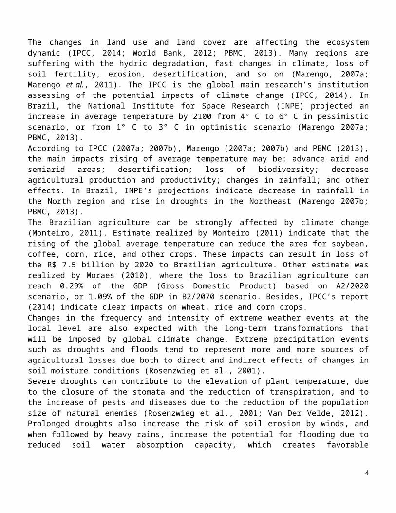
Finally, Figures 6 and 7 present the marginal effects of extreme events on orange production. Production is concentrated in the group agriculture/forest with high-technology, and tends to be negatively impacted by freezes in spring and winter. Extreme heat in the summer and spring also tend to negatively affect the production in the low-technology group, likely due to lack of irrigation. While the marginal effects in the agriculture and agriculture/forest groups present similar levels of heterogeneity, variability is remarkably larger in the urban/pasture group.

Figure 5 – Marginal effects of precipitation below (-) and above (+) the historical average on the log of sugarcane production, São Paulo



The marginal effects of extreme precipitation events on orange production are roughly null in the high technology groups. In turn, these events exhibit diverse impacts in the low technology groups of agriculture

12

and urban/pasture. In other words, no matter the level of technology, orange production is more resilient to extreme precipitation events in areas of agriculture that are integrated with forests.

Figure 6 – Marginal effects of temperature below (-) and above (+) the historical average on the log of orange production, São Paulo



Figure 7 – Marginal effects of precipitation below (-) and above (+) the historical average on the log of orange production, São Paulo



13

5. Discussion

Agricultural production will face relevant challenges from the threats imposed by climate change scenarios. Regions that are highly dependent on natural resources tend to be especially affected by extreme events, since many of them lack the economic and social resources necessary to alleviate the impacts of changes in temperature and precipitation distributions. São Paulo is the most developed state in Brazil, with a significant share of industrial and service activities. Nonetheless, agricultural production plays an important role in the socio-economic dynamics of the state and the country. This is especially the case because the state is the world's leading producer of sugarcane, a strategic crop for the production of sustainable energy (ethanol).

Roughly 70% of São Paulo’s territory is dedicated to agriculture, but municipalities differ substantially in their levels of environmental preservation. The group of municipalities with high environmental preservation (agriculture/forest) have almost 70% of its territory covered by forests and/or mosaics of forests with croplands. Another group of municipalities (agriculture), which feature lower levels of environmental preservation, has 70% of its territory covered exclusively by agriculture and just 17% covered by areas of forests (including mosaics). The last group (urban/pasture) is characterized by the prevalence of urban areas (10%) and by the dichotomy between areas of pasture (25%) and forests (21%).

In addition to environmental preservation, the adoption of production techniques may also play an important role in mitigating the impacts of climate change. As expected, both technological and, especially environmental factors contribute significantly to increases in agricultural productivity: the total value of production is between 15% and 31% higher in the group agriculture/forest when compared to the group agriculture. In turn, the adoption of production practices seems to be more effective in increasing the total value of production when agriculture is practiced with low levels of environmental preservation (i.e. the agriculture group).

The impacts of extreme temperature and precipitation events on agricultural production differ across crops and groups of localities. Sugarcane is more resilient to climate change, while orange production appears to be especially affected by extreme temperatures. In turn, orange production is more resilient to extreme precipitation events in areas of agriculture integrated with forests. Overall, extreme temperature and precipitation events tend to cause more severe impacts (positive or negative) on the total value of production for those groups that feature lower levels of integration between agriculture and environmental preservation (agriculture and urban/pasture). In other words, the group of agriculture integrated with mosaics of forests tends to be more resilient to extreme events.

Finally, we highlight that technologies are necessary but not sufficient to mitigate the impacts of climate change on agricultural development. This is particularly true because degraded areas can disrupt the surface water balance and compromise the adoption of irrigation systems. Furthermore, degraded ecosystem conditions may indirectly introduce pests and pathogens, reduce the benefits of natural pollination, and create a warmer and drier local climate. Farms may introduce technologies and shift to more resilient activities in order to overcome environmental constraints (as sugarcane cultivators have done in São Paulo (Filho and Gasques 2016)), and preserved areas have shown themselves to be related to more profitable and resilient agricultural production. In this sense, sustainable agricultural development policies must prioritize both (i) the adoption of technologies to overcome climate change, such as more resistant seeds and improved land management practices, and (ii) programs of preservation and recuperation of ecosystem services, especially in areas that already face high levels of anthropic intervention.

ReferencesBORRVALL, C., EBENMAN, B. Biodiversity and persistence of ecological communities in variable environments. Ecological Complexity, v. 5, p. 99-105, 2008.

14

Crivisqui, E. 1999. “Presentación de Los Métodos de Clasificación.”

Filho, José Eustáqui Ribeiro Vieira, and José Garcia Gasques. 2016. Agricultura, Transformação Produtiva E Sustentabilidade. Brasília: IPEA.

Foley, Jonathan a, Ruth Defries, Gregory P Asner, Carol Barford, Gordon Bonan, Stephen R Carpenter, F Stuart Chapin, et al. 2005. “Global Consequences of Land Use.” Science 309 (5734): 570–74. doi:10.1126/science.1111772.

IPCC. 2014. Climate Change 2014: Synthesis Report. Contribution of Working Groups I, II and III to the Fifth Assessment Report of the Intergovernmental Panel on Climate Change. IPCC.

DEELSTRA, J. et al. Climate change and runnoff from agricultural catchments in Norway. International Journal of Climate Change Strategies and Management, v. 3, p. 345-360, 2011.

INTERGOVERNMENTAL PANEL ON CLIMATE CHANGE – IPCC (2014). Fifth Assessment Report – AR5. Available at: <http://www.ipcc.ch/report/ar5/>. Accessed on July 20, 2016.

INTERGOVERNMENTAL PANEL ON CLIMATE CHANGE – IPCC (2007a). Fourth Assessment Report – AR4. Available at: <http://www.ipcc.ch/report/ar4/>. Accessed on: July 20, 2016.

INTERGOVERNMENTAL PANEL ON CLIMATE CHANGE – IPCC (2007b). Climate change 2007: the physical science basis. Available at: <http://goo.gl/7bWqXH>. Accessed on: July 20, 2016.

JORGENSEN, S., TERMANSEN, M. Linking climate change perceptions to adaptation and mitigations action. Climatic Change, v. 138, p. 283-296, 2016.

KNAPP, A. K. et al. Consequences of More Extreme Precipitation Regimes for Terrestrial Ecosystems. v. 58, n. 9, p. 811–821, 2008

Kim, Jae-on., and Charles W. Mueller. 1978. Factor Analysis : Statistical Methods and Practical Issues. SAGE Publications.

KUSTURA, A. et al. Soil erosion by water in perennial plantations of Ilok region. Agric. conspec. sci, v. 73, p. 75-83, 2008.

Marengo, Jose A., Tercio Ambrizzi, Rosmeri P. da Rocha, Lincoln M. Alves, Santiago V. Cuadra, Maria C. Valverde, Roger R. Torres, Daniel C. Santos, and Simone E T Ferraz. 2010. “Future Change of Climate in South America in the Late Twenty-First Century: Intercomparison of Scenarios from Three Regional Climate Models.” Climate Dynamics 35 (6): 1089–1113. doi:10.1007/s00382-009-0721-6.

Marengo, Jose A., Sin Chan Chou, Gillian Kay, Lincoln M. Alves, José F. Pesquero, Wagner R. Soares, Daniel C. Santos, et al. 2012. “Development of Regional Future Climate Change Scenarios in South America Using the Eta CPTEC/HadCM3 Climate Change Projections: Climatology and Regional Analyses for the Amazon, São Francisco and the Paraná River Basins.” Climate Dynamics 38 (9–10). Springer-Verlag: 1829–48. doi:10.1007/s00382-011-1155-5.

MARENGO, J. A. (2007a). Mudanças climáticas globais e seus efeitos sobre a biodiversidade. 2ª edição, Brasília-DF, 2007.

MARENGO, J. A. (2007b). Relatório 1: caracterização do clima no século XX e cenários no Brasil e na América do Sul para o século XXI derivados dos Modelos de Clima do IPCC. Available at: <www.inpe.br>. Accessed on: July 20, 2016.

MONTEIRO, F. E. B. de A. Mudança climática será nociva para a agricultura na maior parte do Brasil. Gazeta, Bento Gonçalves, p. 9, 24/05/2011. Available at: <http://www. agrosoft.org.br>. Accessed on: July 16, 2016.

15

MORAES, G. I. de. Efeitos econômicos de cenários de mudança climática na agricultura brasileira: um exercício a partir de um modelo de equilíbrio geral computável. Tese (doutorado em Economia Aplicada), Escola Superior de Agricultura “Luiz de Queiroz”, Universidade de São Paulo, Piracicaba-SP, 2010, fls. 267. Available at: <http://goo.gl/qZYw1X>. Accessed on: July 20, 2016.

MARIOTTE, P. et al. Subordinate plant species enhance community resistance against drought in semi-natural grasslands. Journal of Ecology, v. 101, p. 763-773, 2013.

MARIOTTE, P. et al. Subordinate plants mitigate drought effect on soil ecosystem processes by stimulating fungi. Funcional Ecology, v. 29, p. 1578-1586, 2015.

Mendelsohn, Robert, and Ariel Dinar. 2009. Climate Change and Agriculture: An Economic Analysis of Global Impacts, Adaptation and Distributional Effects. Cheltenham: Edward Elgar.

NAEEM, D., LI, S. Biodiversity enhances ecosystem reliability. Nature, v. 390, p. 507-509,1997.

NEPSTAD, D. The role of deep roots in hydrological and carbon cycles of Amazonian forests and pastures. Nature, v. 372, p. 666-669, 1994.

Painel Brasileiro de Mudanças Climáticas – PBMC. Base científica das mudanças climáticas, volume 1 – primeiro relatório de avaliação nacional. COPPE, Universidade Federal do Rio de Janeiro, Rio de Janeiro, RJ, 2014.

PAINEL BRASILEIRO DE MUDANÇAS CLIMÁTICAS – PBMC (2013). Volume Especial – Primeiro Relatório de Avaliação Nacional. Sumário Executivo. Available at: <http://www.pbmc.coppe.ufrj.br>. Accessed on: July 18, 2016.

PBMC. 2014. Base Científica Das Mudanças climáticas.Base Científica Das Mudanças Climáticas. Contribuição Do Grupo de Trabalho 1 Do Painel Brasileiro de Mudanças Climáticas Ao Primeiro Relatório Da Avaliação Nacional Sobre Mudanças Climáticas. Edited by Tércio Ambrizzi and Moacir Araujo. COPPE, Universidade Federal do Rio de Janeiro, Rio de Janeiro. doi:10.13140/RG.2.1.1641.6883.

ROSENZWEIG, C. et al. Climate change and extreme weather events - Implications for food production, plant diseases, and pests. 2001.

The World Bank. 2012. “Turn Down the Heat: Why a 4°C Warmer World Must Be Avoided.” … Report for the World …, 106.

VÁRALLYAY, G. The impact of climate change on soils an on their water management. Agronomy Research, v. 8, p. 385-396, 2010

VAN DER VELDE, M. et al. Impacts of extreme weather on wheat and maize in France: Evaluating regional crop simulations against observed data. Climatic Change, v. 113, n. 3–4, p. 751–765, 2012

Vergara, Walter. 2009. “Assessing the Potential Consequences of Climate Destabilization in Latin America.” 32. Latin America and Caribbean Region Sustainable Development Working Paper. Washington, DC.

Wreford, Anita, Dominic Moran, and Neil Adger. 2010. Climate Change and Agriculture: Impacts, Adaptation and Mitigation. Source OECD Agriculture & Food, Volume 9.

WORLD BANK (2012). 4° turn down the heat: why a 4 °C warmer world must be avoided? A report for the World Bank by the Potsdam Institute for Climate Impact Research and Climate Analytics. Available at: <http://documents.worldbank.org>. Accessed on: July 20, 2016.

YACHI D., LOREAU, M. Biodiversity and ecosystem productivity in fluctuating environment: The insurance hypothesis, v. 96, p. 1463-1468, 1999.

16

Appendix A

Factor Pattern and Scoring coefficient for the first common factorProduction Technique

Factor Pattern

Scoring Coefficient

Irrigation system 0.402 0.146Sowing machine 0.697 0.252Plowing machine 0.859 0.311Tractor 0.870 0.315Other machines 0.610 0.221Soil treatment 0.500 0.181

Source Elaborated by the authors using data from LUPA

17

Appendix B - Marginal effects of the fixed effects model for the log of total value of production, São Paulo

VariableAgriculture Agriculture/Forest Urban/Pasture

High Low High Low High LowIntercept 1.306 0.950 1.393 2.231 2.260 3.620

(0.291) (0.320) (0.314) (0.229) (0.297) (0.228)

log Area 0.958 0.992 0.946 0.914 0.910 0.808(0.020) (0.021) (0.021) (0.015) (0.030) (0.015)

Tp + 0.015 + 0.005 + -0.005 + -0.008 + 0.117 0.125(0.018) (0.025) (0.021) (0.018) (0.047) (0.026)

Ts + -0.042 -0.068 -0.004 + -0.024 + -0.156 -0.026 +(0.019) (0.027) (0.021) (0.017) (0.048) (0.026)

Ta + -0.029 + -0.055 0.041 0.013 + 0.012 + 0.017 +(0.023) (0.033) (0.025) (0.022) (0.056) (0.032)

Tw + 0.002 + 0.059 0.007 + 0.031 -0.023 + 0.014 +(0.019) (0.027) (0.021) (0.018) (0.048) (0.026)

Tp -0.092 -0.125 -0.035 + 0.027 + 0.021 + -0.153(0.043) (0.056) (0.049) (0.041) (0.169) (0.084)

Ts 0.028 + 0.047 + -0.037 + -0.028 + 0.137 + 0.045 +(0.037) (0.052) (0.041) (0.035) (0.129) (0.058)

Ta 0.055 0.119 0.082 0.052 + 0.067 + 0.055 +(0.029) (0.046) (0.039) (0.037) (0.142) (0.062)

Tw 0.007 + 0.056 + -0.013 + -0.128 -0.037 + -0.131(0.030) (0.039) (0.035) (0.030) (0.084) (0.051)

Pp + 0.007 + 0.022 + 0.045 -0.036 0.033 + 0.105(0.020) (0.027) (0.026) (0.022) (0.047) (0.029)

Ps + 0.003 + -0.022 + 0.038 0.009 + 0.011 + 0.003 +(0.016) (0.023) (0.020) (0.018) (0.041) (0.024)

Pa + 0.008 + -0.009 + -0.019 + 0.004 + 0.003 + 0.002 +(0.017) (0.025) (0.022) (0.018) (0.046) (0.024)

Pw + -0.010 + -0.059 + -0.032 + -0.070 0.056 + 0.052 +(0.027) (0.041) (0.032) (0.027) (0.060) (0.032)

Pp -0.021 + -0.031 + 0.042 0.050 -0.010 + 0.044(0.016) (0.023) (0.021) (0.018) (0.047) (0.024)

Ps -0.017 + -0.035 + -0.020 + -0.017 + -0.040 + -0.012 +(0.018) (0.030) (0.023) (0.020) (0.054) (0.027)

Pa 0.012 + -0.024 + 0.016 + 0.003 + 0.146 -0.038 +(0.021) (0.031) (0.027) (0.022) (0.060) (0.030)

Pw -0.043 0.035 + -0.011 + -0.037 + 0.043 + -0.021 +(0.026) (0.039) (0.029) (0.025) (0.071) (0.036)

n cross section 91 54 107 135 42 124n time series 25 25 25 25 25 25

Source: Elaborated by the authors using data from PAM, IBGE, INMET and LUPA. Standard deviations between parentheses. + Insignificant at 10% level.

18

Appendix C - Marginal effects of the fixed effects model for the log of sugarcane production, São Paulo



(0.070) (0.112) (0.112) (0.094) (0.136) (0.209)

log Area 0.981 1.100 1.026 1.045 1.003 0.980(0.004) (0.007) (0.007) (0.006) (0.010) (0.014)

Tp + 0.015 -0.002 + 0.011 + 0.025 0.065 0.013 +(0.009) (0.015) (0.016) (0.015) (0.033) (0.044)

Ts + -0.008 + -0.004 + -0.012 + 0.004 + -0.027 + 0.073(0.009) (0.015) (0.016) (0.014) (0.031) (0.040)

Ta + 0.005 + -0.010 + 0.001 + -0.005 + 0.009 + 0.018 +(0.011) (0.020) (0.019) (0.018) (0.040) (0.055)

Tw + 0.018 0.033 0.017 + -0.001 + 0.038 + 0.008 +(0.009) (0.016) (0.016) (0.014) (0.033) (0.039)

Tp -0.018 + -0.076 -0.004 + 0.056 -0.095 + -0.008 +(0.020) (0.032) (0.036) (0.033) (0.174) (0.196)

Ts 0.001 + 0.036 + -0.028 + 0.033 + 0.231 -0.061 +(0.018) (0.030) (0.030) (0.029) (0.088) (0.092)

Ta 0.003 + 0.032 + 0.013 + 0.016 + 0.023 + 0.091 +(0.014) (0.027) (0.029) (0.030) (0.119) (0.117)

Tw 0.010 + -0.024 + -0.006 + 0.005 + -0.076 + 0.036 +(0.014) (0.023) (0.027) (0.026) (0.070) (0.088)

Pp + -0.012 + 0.012 + 0.005 + 0.013 + -0.020 + 0.032 +(0.010) (0.016) (0.019) (0.017) (0.030) (0.044)

Ps + 0.015 -0.011 + 0.031 0.003 + -0.010 + 0.010 +(0.008) (0.014) (0.015) (0.014) (0.028) (0.035)

Pa + -0.002 + 0.033 -0.027 + -0.018 + 0.008 + -0.038 +(0.008) (0.015) (0.016) (0.014) (0.033) (0.038)

Pw + -0.006 + 0.003 + -0.002 + 0.020 + 0.042 + -0.002 +(0.013) (0.024) (0.026) (0.023) (0.045) (0.055)

Pp -0.001 + 0.006 + 0.025 + 0.009 + 0.040 + -0.076(0.008) (0.014) (0.016) (0.013) (0.030) (0.038)

Ps 0.002 + 0.005 + -0.016 + 0.002 + 0.036 + 0.041 +(0.009) (0.017) (0.017) (0.015) (0.036) (0.042)

Pa 0.006 + -0.024 + -0.023 + 0.018 + -0.029 + -0.027 +(0.010) (0.018) (0.020) (0.017) (0.039) (0.044)

Pw -0.019 + 0.010 + 0.002 + 0.037 -0.050 + 0.010 +(0.013) (0.023) (0.022) (0.019) (0.050) (0.057)



19

Appendix D - Marginal effects of the fixed effects model for the log of orange production, São Paulo



(0.164)

(0.168)

(0.127)

(0.128)

(0.194)

(0.197)

log Area 0.981 1.036 0.981 1.004 0.987 0.935(0.012

)(0.015

)(0.007

)(0.008

)(0.020

)(0.015

)

Tp + 0.046 + 0.000 +-

0.062-

0.061-

0.005 +-

0.010 +(0.030

)(0.038

)(0.022

)(0.024

)(0.057

)(0.034

)

Ts + 0.005 + 0.031 + 0.035 +-

0.066 0.004 + 0.080(0.031

)(0.042

)(0.022

)(0.022

)(0.056

)(0.030

)

Ta +-

0.092-

0.031 + 0.026 +-

0.024 +-

0.191 0.068(0.035

)(0.047

)(0.026

)(0.028

)(0.069

)(0.038

)

Tw +-

0.036 + 0.060 +-

0.009 + 0.028 + 0.025 + 0.021 +(0.032

)(0.043

)(0.022

)(0.024

)(0.054

)(0.030

)

Tp -

0.001 +-

0.090 +-

0.147-

0.029 +-

0.185 +-

0.132 +(0.060

)(0.074

)(0.050

)(0.052

)(0.176

)(0.124

)

Ts 0.037 + 0.049 + 0.023 +-

0.030 + 0.344-

0.038 +(0.054

)(0.080

)(0.043

)(0.049

)(0.196

)(0.081

)

Ta 0.064 +-

0.048 +-

0.059 +-

0.054 +-

0.021 +-

0.063 +(0.041

)(0.060

)(0.041

)(0.048

)(0.195

)(0.083

)

Tw -

0.032 +-

0.019 +-

0.066-

0.048 +-

0.081 +-

0.035 +(0.046

)(0.058

)(0.038

)(0.040

)(0.110

)(0.070

)

Pp + 0.010 + 0.031 +-

0.027 + 0.023 + 0.079 + 0.005 +(0.031

)(0.039

)(0.027

)(0.028

)(0.059

)(0.033

)

Ps + 0.023 + 0.018 + 0.013 +-

0.010 + 0.008 +-

0.035 +(0.026

)(0.036

)(0.021

)(0.022

)(0.047

)(0.029

)

Pa +-

0.010 +-

0.021 + 0.056 0.011 +-

0.041 + 0.043 +(0.027

)(0.038

)(0.022

)(0.023

)(0.053

)(0.028

)

Pw + 0.022 + - + 0.004 + 0.001 + - + 0.059 +

20

0.077 0.021(0.041

)(0.063

)(0.034

)(0.034

)(0.072

)(0.040

)

Pp -

0.059 0.017 +-

0.004 +-

0.019 +-

0.056 +-

0.012 +(0.026

)(0.035

)(0.022

)(0.022

)(0.053

)(0.027

)

Ps -

0.062 0.090-

0.014 + 0.022 + 0.030 +-

0.022 +(0.030

)(0.046

)(0.024

)(0.024

)(0.061

)(0.032

)

Pa 0.030 +-

0.083 0.066 0.019 + 0.000 + 0.001 +(0.034

)(0.048

)(0.029

)(0.029

)(0.071

)(0.035

)

Pw 0.023 + 0.016 + 0.023 + 0.019 +-

0.063 +-

0.020 +(0.040

)(0.056

)(0.031

)(0.033

)(0.080

)(0.040

)



21

Documents

€¦ · Web viewSome important consequences of anthropic changes in land use and land cover in South America have ... 2012; The World Bank ... on wheat, rice and corn crops