eclass.uoa.gr€¦ · Web viewPRINCIPLES OF HEALTH ECONOMICS. for non-economists. Xavier Martinez-Giralt January 2008. This version March 2010. CODE. Center for …

PRINCIPLES OF HEALTH ECONOMICSfor non-economists

Xavier Martinez-Giralt

January 2008This version March 2010

CODECenter for the study of Organizations

and Decisions in Economics

Copyright Oc 2008 Xavier Martinez-Giralt.Permission is granted to copy, distribute and/or modify this document under the terms of the GNU Free Documentation

License, Version 1.2 or any later version published by the Free Software Foundation; with the Invariant Sections, with the

Front-Cover Texts, and with the Back-Cover Texts. A copy of the license is included in the section entitled “GNU Free

Documentation License”.

HEALTH ECONOMICS

1. Economics and Health Economics

1.1 What is economics about?1.2 What is health economics? Elements of HE;

Organization, actors of the health care market; Structure of a health care system

2. The agents of the economy

2.1 Demand: consumers, patients, elasticity2.2 Supply: firms, hospitals physicians;

Efficiency, Efficacy, Effectiveness, Equity, Opportunity cost

2.3 Insurers

3. The market and the health care market

3.1 Why is the health care market different?3.2 Perfectly competitive markets

4. Regulation

4.1 The public sector4.2 Mechanisms of regulation4.3 Reasons for regulation4.4 Regulation in the health care market

5. Public goods

6. Nonprofit organizations

6.1 Why do nonprofit enterprises exist?6.2 Modeling a nonprofit hospital

7. A health policy exercise

8. Uncertainty, risk and insurance

8.1 Attitudes facing risk8.2 Health insurance

9. Contract theory

9.1 Contracts, information and agency relation9.2 Adverse selection, moral hazard and signalling9.3 Supplier induced demand

10. Economic evaluation

10.1 QALYs10.2 Components in economic evaluation10.3 CEA, CUA, CBA

11. Macroeconomics

11.1 What is macroeconomics about?11.2 The working of the economy11.3 Macroeconomics of the health sector

References

Deeming, C., and J. Keen, 2004, Choice and equity: lessons from long term care, British Medical Journal, 328: 1390- 1391.

Drummond, M.F., B, O’Brien, G.L. Stoddart y G.W. Torrance, 2003, Methods for the economic evaluation of health care programmes, Oxford University Press, Oxford

Feldstein, P.J., 2004, Health Care Economics, Thomson, Lon- don.

Folland, S., A.C. Goodman, and M. Stano, 2009, The Eco- nomics of Health and Health Care, Pearson Education, Upper Saddle River, New Jersey.

Jacobs, P., 2003, The Economics of Health and Medical Care, Jones and Bartlett Publishers.

Jones, A.M., 2006, The Elgar Companion to Health Economics, Cheltenham, Edward Elgar.

Keating, B., 2008, Microeconomics for Public Managers, Black- well, London.

Lewis, T.R., J.H. Reichman, and A.D. So, 2007, The case forpublic funding and public oversight of clinical trials, Economists’ Voice, January.

Macho Stadler, I. and J. D. Pe´rez Castrillo, 2001, An Introduc- tion to the Economics of Information, New York, Oxford University Press.

McGuire, A., J. Henderson, and G. Mooney, 1995, The Eco- nomics of Health Care, Routledge, London.

Phelps, C.E., 2009, Health Economics, Addison Wesley, New York.

Porter, M.E., and E.O. Teisberg, 2006, Redefining Health Care, Boston (Ma.), Harvard Business School.

Santerre, R.E., and S.P. Neun, 2004, Health Economics, Thom- son, London.

Wonderling, D., R. Gruen, and N. Black, 2005, Introduction to Health Economics, Open University Press, Maidenhead, Berkshire.

Zweifel, P., F. Breyer, and M. Kifmann, 2009, Health Eco- nomics, Springer, London.

O

GNU Free Documentation License

Version 1.2, November 2002Copyright c 2000,2001,2002 Free Software Foundation, Inc. 59 Temple Place, Suite 330, Boston, MA 02111-1307 USA

Everyone is permitted to copy and distribute verbatim copies of this license document, but changing it is not allowed.

Preamble

The purpose of this License is to make a manual, textbook, or other functional and useful document ”free” in the sense of freedom: to assure everyone the effective freedom to copy and redistribute it, with or without modifying it, either commercially or noncommercially. Secondarily, this License preserves for the author and publisher a way to get credit for their work, while not being considered responsible for modifications made by others.

This License is a kind of ”copyleft”, which means that derivative works of the document must themselves be free in the same sense. It complements the GNU General Public License, which is a copyleft license designed for free software.

We have designed this License in order to use it for manuals for free software, because free software needs free documentation: a free program should come with manuals providing the same freedoms that the software does. But this License is not limited to software manuals; it can be used for any textual work, regardless of subject matter or whether it is published as a printed book. We recommend this License principally for works whose purpose is instruction or reference.

1 Applicability and Definitions

This License applies to any manual or other work, in any medium, that contains a notice placed by the copyright holder saying it can be distributed under the terms

of this License. Such a notice grants a world-wide, royalty-free license, unlimited in duration, to use that work under the conditions stated herein. The ”Document”, below, refers to any such manual or work. Any member of the public is a licensee, and is addressed as ”you”. You accept the license if you copy, modify or distribute the work in a way requiring permission under copyright law.

A ”Modified Version” of the Document means any work containing the Doc- ument or a portion of it, either copied verbatim, or with modifications and/or trans- lated into another language.

A ”Secondary Section” is a named appendix or a front-matter section of the Document that deals exclusively with the relationship of the publishers or authors of the Document to the Document’s overall subject (or to related matters) and contains nothing that could fall directly within that overall subject. (Thus, if the Doc- ument is in part a textbook of mathematics, a Secondary Section may not explain any mathematics.) The relationship could be a matter of historical connection with the subject or with related matters, or of legal, commercial, philosophical, ethical or political position regarding them.

The ”Invariant Sections” are certain Secondary Sections whose titles are designated, as being those of Invariant Sections, in the notice that says that the Docu- ment is released under this License. If a section does not fit the above definition of Secondary then it is not allowed to be designated as Invariant. The Document may contain zero Invariant Sections. If the Document does not identify any Invariant Sections then there are none.

The ”Cover Texts” are certain short passages of text that are listed, as Front- Cover Texts or Back-Cover Texts, in the notice that says that the Document is released under this License. A Front-Cover Text may be at most 5 words, and a Back-Cover Text may be at most 25 words.

A ”Transparent” copy of the Document means a machine-readable copy, rep- resented in a format whose specification is available to the general public, that is suitable for revising the document straightforwardly with generic text editors or (for images composed of pixels) generic paint programs or (for drawings) some widely available drawing editor, and that is suitable for input to text formatters or for automatic translation to a variety of formats suitable for input to text formatters. A copy made in an otherwise Transparent file format whose markup, or absence of markup, has been arranged to thwart or discourage subsequent modification by readers is not Transparent. An image format is not Transparent if used for any substantial amount of text. A copy that is not ”Transparent” is called ”Opaque”.

Examples of suitable formats for Transparent copies include plain ASCII without markup, Texinfo input format, LaTeX input format, SGML or XML using a publicly available DTD, and standard-conforming simple HTML, PostScript or PDF designed for human modification. Examples of transparent image formats include PNG, XCF and JPG. Opaque formats include proprietary formats that can be read and edited only by proprietary word processors, SGML or XML for which the DTD and/or processing tools are not generally available, and the machine- generated HTML, PostScript or PDF produced by some word processors for output

purposes only.The ”Title Page” means, for a printed book, the title page itself, plus such

following pages as are needed to hold, legibly, the material this License requires to appear in the title page. For works in formats which do not have any title page as such, ”Title Page” means the text near the most prominent appearance of the work’s title, preceding the beginning of the body of the text.

A section ”Entitled XYZ” means a named subunit of the Document whose title either is precisely XYZ or contains XYZ in parentheses following text that trans- lates XYZ in another language. (Here XYZ stands for a specific section name men- tioned below, such as ”Acknowledgements”, ”Dedications”, ”Endorsements”, or ”History”.) To ”Preserve the Title” of such a section when you modify the Document means that it remains a section ”Entitled XYZ” according to this definition.

The Document may include Warranty Disclaimers next to the notice which states that this License applies to the Document. These Warranty Disclaimers are considered to be included by reference in this License, but only as regards dis- claiming warranties: any other implication that these Warranty Disclaimers may have is void and has no effect on the meaning of this License.

2 Verbatim Copying

You may copy and distribute the Document in any medium, either commercially or noncommercially, provided that this License, the copyright notices, and the license notice saying this License applies to the Document are reproduced in all copies, and that you add no other conditions whatsoever to those of this License. You may not use technical measures to obstruct or control the reading or further copying of the copies you make or distribute. However, you may accept compensation in exchange for copies. If you distribute a large enough number of copies you must also follow the conditions in section 3.

You may also lend copies, under the same conditions stated above, and you may publicly display copies.

3 Copying in Quantity

If you publish printed copies (or copies in media that commonly have printed covers) of the Document, numbering more than 100, and the Document’s license notice requires Cover Texts, you must enclose the copies in covers that carry, clearly and legibly, all these Cover Texts: Front-Cover Texts on the front cover, and Back- Cover Texts on the back cover. Both covers must also clearly and legibly identify you as the publisher of these copies. The front cover must present the full title with all words of the title equally prominent and visible. You may add other material on the covers in addition. Copying with changes limited to the covers, as long as they

preserve the title of the Document and satisfy these conditions, can be treated as verbatim copying in other respects.

If the required texts for either cover are too voluminous to fit legibly, you should put the first ones listed (as many as fit reasonably) on the actual cover, and continue the rest onto adjacent pages.

If you publish or distribute Opaque copies of the Document numbering more than 100, you must either include a machine-readable Transparent copy along with each Opaque copy, or state in or with each Opaque copy a computer-network location from which the general network-using public has access to download using public-standard network protocols a complete Transparent copy of the Document, free of added material. If you use the latter option, you must take reasonably pru- dent steps, when you begin distribution of Opaque copies in quantity, to ensure that this Transparent copy will remain thus accessible at the stated location until at least one year after the last time you distribute an Opaque copy (directly or through your agents or retailers) of that edition to the public.

It is requested, but not required, that you contact the authors of the Document well before redistributing any large number of copies, to give them a chance to provide you with an updated version of the Document.

4 Modifications

You may copy and distribute a Modified Version of the Document under the conditions of sections 2 and 3 above, provided that you release the Modified Version under precisely this License, with the Modified Version filling the role of the Docu- ment, thus licensing distribution and modification of the Modified Version to who- ever possesses a copy of it. In addition, you must do these things in the Modified Version:

A. Use in the Title Page (and on the covers, if any) a title distinct from that of the Document, and from those of previous versions (which should, if there were any, be listed in the History section of the Document). You may use the same title as a previous version if the original publisher of that version gives permission.

B. List on the Title Page, as authors, one or more persons or entities responsible for authorship of the modifications in the Modified Version, together with at least five of the principal authors of the Document (all of its principal authors, if it has fewer than five), unless they release you from this requirement.

C. State on the Title page the name of the publisher of the Modified Version, as the publisher.

D. Preserve all the copyright notices of the Document.

E. Add an appropriate copyright notice for your modifications adjacent to the other copyright notices.

F. Include, immediately after the copyright notices, a license notice giving the public permission to use the Modified Version under the terms of this Li- cense, in the form shown in the Addendum below.

G. Preserve in that license notice the full lists of Invariant Sections and required Cover Texts given in the Document’s license notice.

H. Include an unaltered copy of this License.

I. Preserve the section Entitled ”History”, Preserve its Title, and add to it an item stating at least the title, year, new authors, and publisher of the Modified Version as given on the Title Page. If there is no section Entitled ”History” in the Document, create one stating the title, year, authors, and publisher of the Document as given on its Title Page, then add an item describing the Modified Version as stated in the previous sentence.

J. Preserve the network location, if any, given in the Document for public access to a Transparent copy of the Document, and likewise the network locations given in the Document for previous versions it was based on. These may be placed in the ”History” section. You may omit a network location for a work that was published at least four years before the Document itself, or if the original publisher of the version it refers to gives permission.

K. For any section Entitled ”Acknowledgements” or ”Dedications”, Preserve the Title of the section, and preserve in the section all the substance and tone of each of the contributor acknowledgements and/or dedications given therein.

L. Preserve all the Invariant Sections of the Document, unaltered in their text and in their titles. Section numbers or the equivalent are not considered part of the section titles.

M. Delete any section Entitled ”Endorsements”. Such a section may not be included in the Modified Version.

N. Do not retitle any existing section to be Entitled ”Endorsements” or to conflict in title with any Invariant Section.

O. Preserve any Warranty Disclaimers.

If the Modified Version includes new front-matter sections or appendices that qualify as Secondary Sections and contain no material copied from the Document, you may at your option designate some or all of these sections as invariant. To do this, add their titles to the list of Invariant Sections in the Modified Version’s license notice. These titles must be distinct from any other section titles.

You may add a section Entitled ”Endorsements”, provided it contains nothing but endorsements of your Modified Version by various parties–for example, state- ments of peer review or that the text has been approved by an organization as the authoritative definition of a standard.

You may add a passage of up to five words as a Front-Cover Text, and a passage of up to 25 words as a Back-Cover Text, to the end of the list of Cover Texts in the Modified Version. Only one passage of Front-Cover Text and one of Back-Cover Text may be added by (or through arrangements made by) any one entity. If the Document already includes a cover text for the same cover, previously added by you or by arrangement made by the same entity you are acting on behalf of, you may not add another; but you may replace the old one, on explicit permission from the previous publisher that added the old one.

The author(s) and publisher(s) of the Document do not by this License give permission to use their names for publicity for or to assert or imply endorsement of any Modified Version.

5 Combining Documents

You may combine the Document with other documents released under this License, under the terms defined in section 4 above for modified versions, provided that you include in the combination all of the Invariant Sections of all of the original documents, unmodified, and list them all as Invariant Sections of your combined work in its license notice, and that you preserve all their Warranty Disclaimers.

The combined work need only contain one copy of this License, and multiple identical Invariant Sections may be replaced with a single copy. If there are multiple Invariant Sections with the same name but different contents, make the title of each such section unique by adding at the end of it, in parentheses, the name of the original author or publisher of that section if known, or else a unique number. Make the same adjustment to the section titles in the list of Invariant Sections in the license notice of the combined work.

In the combination, you must combine any sections Entitled ”History” in the various original documents, forming one section Entitled ”History”; likewise combine any sections Entitled ”Acknowledgements”, and any sections Entitled ”Dedi- cations”. You must delete all sections Entitled ”Endorsements”.

6 Collections of Documents

You may make a collection consisting of the Document and other documents released under this License, and replace the individual copies of this License in the various documents with a single copy that is included in the collection, provided that you follow the rules of this License for verbatim copying of each of the documents in all other respects.

You may extract a single document from such a collection, and distribute it individually under this License, provided you insert a copy of this License into the extracted document, and follow this License in all other respects regarding verbatim copying of that document.

7 Aggregation With Independent Works

A compilation of the Document or its derivatives with other separate and independent documents or works, in or on a volume of a storage or distribution medium, is called an ”aggregate” if the copyright resulting from the compilation is not used to limit the legal rights of the compilation’s users beyond what the individual works permit. When the Document is included in an aggregate, this License does not apply to the other works in the aggregate which are not themselves derivative works of the Document.

If the Cover Text requirement of section 3 is applicable to these copies of the Document, then if the Document is less than one half of the entire aggregate, the Document’s Cover Texts may be placed on covers that bracket the Document within the aggregate, or the electronic equivalent of covers if the Document is in electronic form. Otherwise they must appear on printed covers that bracket the whole aggregate.

8 Translation

Translation is considered a kind of modification, so you may distribute translations of the Document under the terms of section 4. Replacing Invariant Sections with translations requires special permission from their copyright holders, but you may include translations of some or all Invariant Sections in addition to the original versions of these Invariant Sections. You may include a translation of this License, and all the license notices in the Document, and any Warranty Disclaimers, provided that you also include the original English version of this License and the original versions of those notices and disclaimers. In case of a disagreement between the translation and the original version of this License or a notice or disclaimer, the original version will prevail.

If a section in the Document is Entitled ”Acknowledgements”, ”Dedications”, or ”History”, the requirement (section 4) to Preserve its Title (section 1) will typi- cally require changing the actual title.

9 Termination

You may not copy, modify, sublicense, or distribute the Document except as ex- pressly provided for under this License. Any other attempt to copy, modify, sublicense or distribute the Document is void, and will automatically terminate your

rights under this License. However, parties who have received copies, or rights, from you under this License will not have their licenses terminated so long as such parties remain in full compliance.

10 Future Revisions of This License

The Free Software Foundation may publish new, revised versions of the GNU Free Documentation License from time to time. Such new versions will be similar in spirit to the present version, but may differ in detail to address new problems or concerns. See http://www.gnu.org/copyleft/.

Each version of the License is given a distinguishing version number. If the Document specifies that a particular numbered version of this License ”or any later version” applies to it, you have the option of following the terms and conditions either of that specified version or of any later version that has been published (not as a draft) by the Free Software Foundation. If the Document does not specify a version number of this License, you may choose any version ever published (not as a draft) by the Free Software Foundation.

1

Qc

Economics

Healthof

inciples Pr

HEALTH ECONOMICS

1. Economics and Health Economics

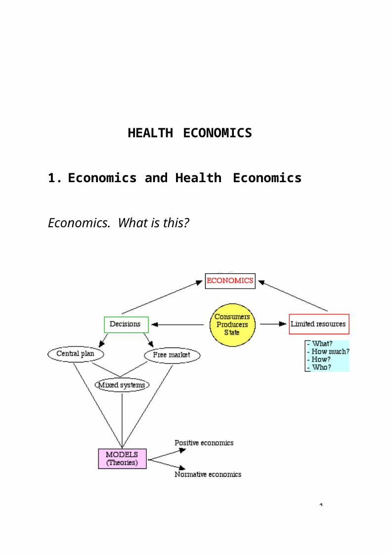
Economics. What is this?

Economics: Study of the way in which economic agents take their decisions regarding the use (allocation) of scarce resources.

Economic agents: Decision makers in the economy. Individuals, households, enterprises (for profit, nonprofit; production, distribution), State.

Decisions:

- what to produce/consume?

- how much to produce/consume?

- How to produce/consume?

- Who produces/consumes?

Answers to these questions depend on the organization of the economy: central plan, free market, mixed systems.

1-a

1-

Reality too complex. Study of an economy by means of models (theories): set of assumptions providing a simplified representation of reality capturing the fundamental relationships among economic agents [→ road map vs. road network].

Two (complementary) uses of models:

- description of decision making process → positive economics

- policy design (control and improvement of decision making) → normative economics

1

Scarcity: wants vs. limited resources

* Why do people demand (want) health care?

(i) Healthy status → Lo income → Lo leisure

1-

alt

tinez-Gir Mar

X

avier

Qc

Health of

inciples Pr

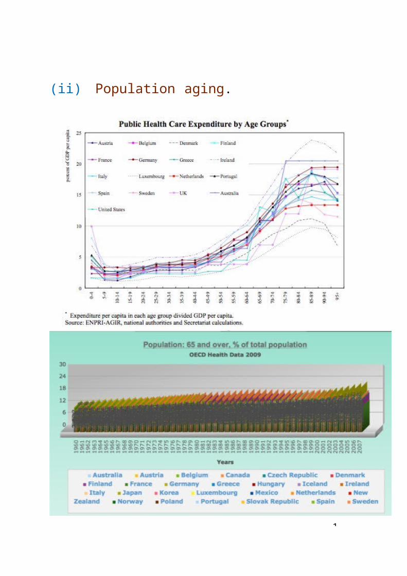
(ii) Population aging.

1-

Economic

s Healthof

inciples Pr

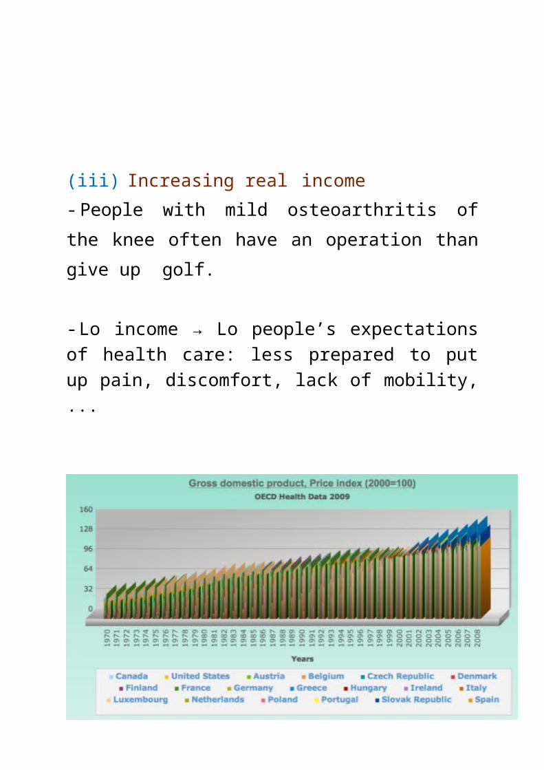
(iii) Increasing real income- People with mild osteoarthritis of the knee often have an operation than give up golf.

- Lo income → Lo people’s expectations of health care: less prepared to put up pain, discomfort, lack of mobility, ...

1

(iv) Improvement in medical technology:

- Technology increases range of possible treatments.

- Newer technology, more expensive

e.g. kidney dialysis → prevent people dying from kidney failure ⇒ machine is expensive, there are more patients (population aging) and they are treated longer (extended life expectancy).

Reading:Cutler, D., E. Glaeser, and A. Rosen, 2007, Is theU.S. Population Behaving Healthier?, NBER Work- ing Paper No. 13013

[http://www.nber.org/papers/w13013]

1-

M

artinez

Xavier

Qc

Economics

Healthof

-G

P

Publications | Research | Data | About | People Login or change prefs

Is the U.S. Population Behaving Healthier?

" Reduced smoking, better control of medical risk factors such as hypertension and cholesterol, and better education among the older population have been more important for mortality than the substantial increase in obesity."

Knowing whether health behaviors are improving over time is important in forecasting medical costs. And, a population that behaves in a healthier way will have a higher quality of life than one with a more adverse behavioral profile, even given length of life. In Is the U.S. Population Behaving Healthier? (NBER Working Paper No. 13013), authors David Cutler, Edward Glaeser, and Allison Rosen consider what has happened to the population's health behaviors over time and what the future may hold.

They find that the impact on longevity of trends in health behavior has not been uniform across different behaviors over the past three decades. For example, while fewer people smoke than used to, more people are obese. Examining these factors as a whole, the authors find significant improvement in the health-risk profile of the U.S. population between the early 1970s and the early 2000s. Reduced smoking, better control of medical risk factors such as hypertension and cholesterol, and better education among the older population have been more important for mortality than the substantial increase in obesity.

The results suggest substantial caution about the future, though. Where reductions in smoking can be expected to have a continued impact on improved health, future changes in obesity might more than overwhelm this trend. Two-thirds of the U.S. population is now overweight or obese. As a result, continued increases in weight from current levels will have a bigger impact on health than did increases in weight from lower levels of Body Mass Index (BMI).

A large part of the impact of BMI is moderated through its effect on hypertension and high cholesterol. Given that not everyone with these conditions takes medications, or is controlled by the medication they do take, the resulting impact of rising weight on health can be significant. The optimistic side of this picture, however, is the potential for better control of obesity. If the effectiveness of risk-factor control can be increased, through more people taking medication and those taking it using it more regularly, much of the impact of obesity on mortality risk can be blunted, according to the authors.

Understanding how to improve utilization of and adherence to recommended medications are key issues in health outcomes. The research to date has focused on two possible avenues. The first is performance-based payment: physicians are now paid for office visits, but not for ensuring follow- up with their recommendations. The idea behind pay-for-performance systems is to reward physicians (or insurance companies) for successful efforts to increase utilization and possibly adherence. Such efforts might involve having nurse outreach, automatic medication refills, or more convenient office hours to monitor side effects.

The second strategy involves use of information technology. Patients can receive electronic reminders about medication goals, information such as blood pressure can be transmitted and monitored electronically, and automated decision tools can help with dosing and medication switches. Whether these or other strategies offer the greatest promise of improved adherence is uncertain. The authors' results suggest that evaluating these strategies in practice is a high research priority.

The authors use as their primary data source the National Health and Nutrition Examination Survey (NHANES). In the United States, it is the leading survey and includes both physical examination and laboratory measurements. The authors use two NHANES surveys, the first from 1971-5 (NHANES I) and the second from 1999-2002 (NHANES IV). Their analysis begins with NHANES I because it is the first population health survey that asked about smoking status, a key variable in health risk.

-- Les Picker

The Digest is not copyrighted and may be reproduced freely with appropriate attribution of source.

1-

* Resources: inputs, factors of production.- land (physical resources of the planet)- labor (human resources)- capital (resources created by human to aid in production: tools, machinery, factories, ...)

enterprise: organization of resources to produce goods and services.

* Main concepts related with scarcity:

Efficiency

Opportunity cost

Production Possibility Frontier

2

⇒→

⇒

→

What is Health Economics?

Allocation of resources within the health system in the economy, as well as the functioning of the health care markets.

health system: set of interrelated elements (environment, education, labor conditions, etc) having as objective the transformation of some sanitary resources (inputs) into a health status (final output) through the production of health care services (intermediate output).

Health vs. Health care:Health is lack of illness illness: restrictions im- posed on the development of daily activities value in use but no value in exchange.Health care: provision of services to improve health status of individuals intermediate output. Can be traded.

healthcare market: interaction between providers and consumers of health care services (and insurers).

Organization of HC market crucial element of analysis of HC system.

2-

Readings:

Rout, H.S., and P.K. Panda, 2007, Health and Health Economics: A conceptual framework, in Health Eco- nomics in India, edited by H.S. Rout, and P.K. Panda, New Century Publications, New Delhi: 13-29.

[http://mpra.ub.uni-muenchen.de/6546]

Chicaiza, L, M. Garc´ıa, and J. Lozano, 2008, Bring- ing Institutions into Health Economics, Documentos de Trabajo - Esc. de Admon. y Con Pub. 004687, Universidad Nacional de Colombia - RCE.

[http://ideas.repec.org/p/col/000179/004687.html]

2-

•

• Lo

Health economics

- Descriptive studies: long tradition

- Analytic studies: (relatively) recent. Stimulated by (EU) Maastricht: difficulties finance universal

public health systems(US) Efforts extend coverage beyond Medicaid and

Medicare - Clinton+Obama administration

Restructure health care sy⇓

stems via- stimulating competition- incentives: principals, agents, payment systems, insurance, risk, etc.

Taking into account the characterisitics of the health care system. (see p. 2n)

Consequences

Health economics as separate discipline from In- dustrial economics:

- scientific journals

- huge volume of resources

2

Why has Health Economics developed into a discipline itself?

Size and differential characteristics of health care sector in the economy.

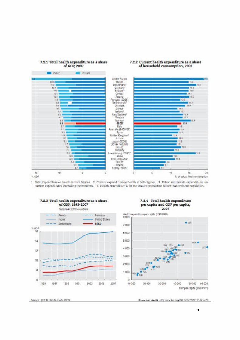
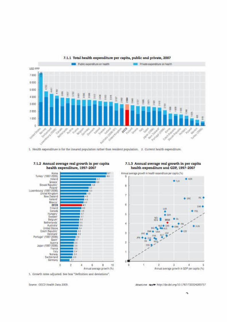
Size

OECD Health Data:

(a) Health expenditure

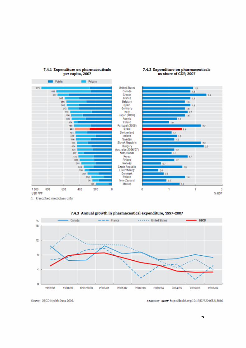
(b) Pharma expenditure

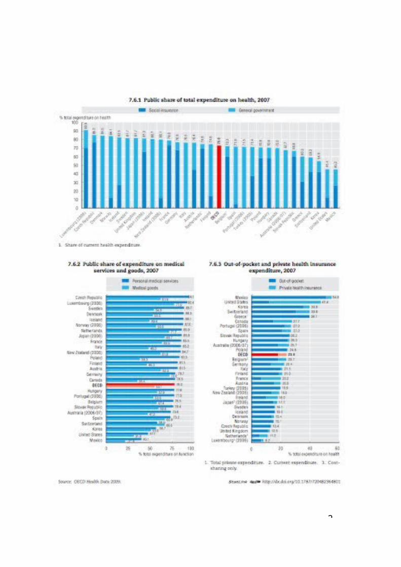
(c) Health financing

(d) Population

2-

Health of

inciples Pr

Total expenditure on health - % of gross domestic product

1960 1965 1970 1975 1980 1985 1990 1995 2000 2001 2002 2003 2004Australia 4.0 4.2 4.5 6.9 6.8 7.2 7.5 8.0 8.8 8.9 9.1 9.2 ..Austria 4.3 4.6 5.2 7.0 7.5 6.5 7.0 9.7 9.4 9.5 9.5 9.6 9.6Belgium .. .. 3.9 5.6 6.3 7.0 7.2 8.2 8.6 8.7 8.9 10.1 ..Canada 5.4 5.9 7.0 7.1 7.1 8.2 9.0 9.2 8.9 9.4 9.7 9.9 9.9Czech Republic .. .. .. .. .. .. 4.7 7.0 6.7 7.0 7.2 7.5 7.3Denmark .. .. 7.9 8.7 8.9 8.5 8.3 8.1 8.3 8.6 8.8 8.9 8.9Finland 3.8 4.8 5.6 6.2 6.3 7.1 7.8 7.4 6.7 6.9 7.2 7.4 7.5France 3.8 4.7 5.3 6.4 7.0 7.9 8.4 9.4 9.2 9.3 10.0 10.4 10.5Germany .. .. 6.2 8.6 8.7 9.0 8.5 10.3 10.4 10.6 10.8 10.9 ..Greece .. .. 6.1 6.6 7.4 7.4 9.6 9.9 10.4 10.3 10.5 10.0Hungary .. .. .. .. .. .. 7.1 7.4 7.1 7.3 7.7 8.3 8.3Iceland 3.0 3.5 4.7 5.7 6.2 7.2 7.9 8.4 9.2 9.3 10.0 10.5 10.2Ireland 3.7 4.0 5.1 7.3 8.3 7.5 6.1 6.7 6.3 6.8 7.2 7.2 7.1Italy .. .. .. .. .. 7.5 7.7 7.1 7.9 8.0 8.2 8.2 8.4Japan 3.0 4.4 4.5 5.6 6.5 6.7 5.9 6.8 7.6 7.8 7.9 8.0 ..Korea .. .. 4.4 4.1 4.4 4.2 4.8 5.4 5.3 5.5 5.6Luxembourg .. .. 3.1 4.3 5.2 5.2 5.4 5.6 5.8 6.4 6.8 7.7 8.0Mexico .. .. .. .. .. .. 4.8 5.6 5.6 6.0 6.2 6.3 6.5Netherlands .. .. 6.6 6.9 7.2 7.1 7.7 8.1 7.9 8.3 8.9 9.1 9.2New Zealand .. .. 5.1 6.5 5.9 5.1 6.9 7.2 7.7 7.8 8.2 8.0 8.4Norway 2.9 3.4 4.4 5.9 7.0 6.6 7.7 7.9 8.5 8.9 9.9 10.1 9.7Poland .. .. .. .. .. .. 4.9 5.6 5.7 6.0 6.6 6.5 6.5Portugal 2.6 5.4 5.6 6.0 6.2 8.2 9.4 9.3 9.5 9.8 10.0Slovak Republic .. .. .. .. .. .. .. 5.8 5.5 5.5 5.6 5.9 ..Spain 1.5 2.5 3.5 4.6 5.3 5.4 6.5 7.4 7.2 7.2 7.3 7.9 8.1Sweden .. .. 6.8 7.6 9.0 8.6 8.3 8.1 8.4 8.7 9.1 9.3 9.1Switzerland 4.9 4.6 5.5 7.0 7.4 7.8 8.3 9.7 10.4 10.9 11.1 11.5 11.6Turkey .. .. .. 3.0 3.3 2.2 3.6 3.4 6.6 7.5 7.4 7.6 7.7United Kingdom 3.9 4.1 4.5 5.5 5.6 5.9 6.0 7.0 7.3 7.5 7.7 7.9 8.3United States 5.1 5.6 7.0 7.9 8.8 10.1 11.9 13.3 13.3 14.0 14.7 15.2 15.3

Source: OECD HEALTH DATA 2006

18.0AustraliaAustria Belgium

16.0 CanadaCzech Republic Denmark

14.0 FinlandFrance Germany

12.0 GreeceHungaryIceland Ireland

10.0 ItalyJapan Korea

8.0 LuxembourgMexico Netherlands

6.0 New ZealandNorwayPoland Portugal

4.0 Slovak RepublicSpain Sweden

2.0 SwitzerlandTurkeyUnited Kingdom United States

0.01960 1965 1970 1975 1980 1985 1990 1995 2000 2001 2002 2003 2004

2-

alt

tinez-Gir Mar

Xavier

Qc

Economics

Healthof

inciples Pr

2

alt

tinez-Gir Mar

Xavier

Qc

Economics

Healthof

inciples Pr

2-

Marvier

Qc

Healthof

HEALTH: SPENDING AND RESOURCESHealth spending and financing

Total expenditure as

% of GDP

Publicexpenditure as

% of total expenditure on

health

Averag e

growth rate

Health expenditure Per capita USD PPP

Pharmaceuticalexpenditure as

% of total expenditure on

health2003 1993 2003 1993 1998-

20032003 1993 2003 1993

Australia 19.3 a 8.2 68 a 66 4.1 d 2 699 a 1 542 14 e 10

Austria 7.6 a 7.8 70 a 74 1.8 d 2 280 a 1 669 16 a 11 h

Belgium 9.6 8.1 .. .. 4.2 2 827 1 601 17 f 17Canada 9.9 b 9.9 70 b 73 4.2 3 003 b 2 014 17 13Czech Republic 7.5 6.7 90 95 5.4 1 298 760 22 19Denmark 9 8.8 83 83 2.8 2 763 1 763 9.8 8.5Finland 7.4 8.3 | 77 76 | 4.1 2 118 1 430 | 16 12France 10 b 9.4 76 b 77 3.5 2 903 b 1 878 21 18Germany 11 9.9 78 80 1.8 2 996 1 988 15 13Greece 9.9 8.8 51 b 55 4.9 2 011 1 077 16 17Hungary 7.8 a 7.7 70 a 87 6 | 1 115 a 638 28 a 28Iceland 11 b 8.4 84 b 83 5.9 3 115 b 1 745 15 12Ireland 7.3 a 7 75 a 73 11 | 2 386 a 1 039 11 a 11Italy 8.4 8 75 76 3.1 2 258 1 529 22 20Japan 7.9 a,b 6.5 82 a,b 79 3 | 2 139 a,b 1 365 18 a 22Korea 5.6 4.3 49 36 10 1 074 453 29 31Luxembourg 6.1 a 6.2 85 a 93 5.3 | 3 190 a 1 891 12 a 12 i

Mexico 6.2 5.8 46 43 4 583 397 21 ..Netherlands 9.8 8.6 62 74 4.6 2 976 1 701 11 11New Zealand 8.1 7.2 79 77 3.4 1 886 1 115 14 f 15Norway 10 b 8 84 b 85 5.3 3 807 b 1 695 9.4 a 9.6Poland 6 a 5.9 72 a 74 3 | 677 a 378 .. ..Portugal 9.6 7.3 70 63 3.7 1 797 881 23 g 26Slovak Republic 5.9 .. 88 .. 4.1 777 .. 39 ..Spain 7.7 7.5 71 77 2.6 1 835 1 089 22 19 h

Sweden 9.2 a 8.6 | 85 a 87 | 5.4 | 2 594 a 1 644 | 13 a 11Switzerland 12 b 9.4 59 b 54 2.8 3 781 b 2 401 11 9.7Turkey 6.6 c 3.7 63 c 66 .. 452 c 200 25 c 32 i

United Kingdom 7.7 a 6.9 83 a 85 5.7 | 2 231 a 1 232 16 f 15United States2

15 13 44 43 4.6 5 635 3 357 13 8.6

Source:: OECD Health Data 2005

2-

Mar

Xavier

Qc

Economics

Healthof

inciples

2

Health of

inciples Pr

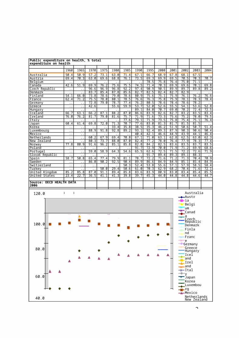
Public expenditure on health, % total expenditure on health

1960 1965 1970 1975 1980 1985 1990 1995 2000 2001 2002 2003 2004Australia 50.4 50.9 57.2 73.1 63.0 71.4 67.1 66.7 68.9 67.8 68.1 67.5 ..Austria 69.4 70.3 63.0 69.6 68.8 76.1 73.5 69.3 69.9 69.5 70.5 70.3 70.7Belgium .. .. .. .. .. .. .. 78.5 75.8 76.4 75.0 71.1 ..Canada 42.6 51.9 69.9 76.2 75.6 75.5 74.5 71.4 70.3 69.9 69.6 70.1 69.8Czech Republic .. .. 96.6 96.9 96.8 92.2 97.4 90.9 90.5 89.9 89.7 89.8 89.2Denmark .. .. 83.7 85.4 87.8 85.6 82.7 82.5 82.4 82.7 82.9 .. ..Finland 54.1 66.0 73.8 78.6 79.0 78.6 80.9 75.6 75.1 75.9 76.1 76.2 76.6France 62.4 71.2 75.5 78.0 80.1 78.5 76.6 76.3 75.8 75.9 78.1 78.3 78.4Germany .. .. 72.8 79.0 78.7 77.4 76.2 80.5 78.6 78.4 78.6 78.2 ..Greece .. .. 42.6 55.6 59.9 53.7 52.0 52.6 55.5 54.1 53.6 52.8Hungary .. .. .. .. .. .. 89.1 84.0 70.7 69.0 70.2 72.4 72.5Iceland 66.7 63.1 66.2 87.1 88.2 87.0 86.6 83.9 82.6 82.7 83.2 83.5 83.4Ireland 76.0 76.2 81.7 79.0 81.6 75.7 71.9 71.6 73.3 75.6 75.2 78.0 79.5Italy .. .. .. .. .. 77.6 79.1 71.9 73.5 75.8 75.4 75.1 76.4Japan 60.4 61.4 69.8 72.0 71.3 70.7 77.6 83.0 81.3 81.7 81.5 81.5 ..Korea .. .. .. .. 33.4 35.8 38.5 35.3 46.2 51.9 50.6 50.7 51.4Luxembourg .. .. 88.9 91.8 92.8 89.2 93.1 92.4 89.3 87.9 90.3 90.6 90.4Mexico .. .. .. .. .. .. 40.4 42.1 46.6 44.9 43.9 44.1 46.4Netherlands .. .. 60.2 67.9 69.4 70.8 67.1 71.0 63.1 62.8 62.5 63.0 62.3New Zealand .. .. 80.3 73.7 88.0 87.0 82.4 77.2 78.0 76.4 77.9 78.3 77.4Norway 77.8 80.9 91.6 96.2 85.1 85.8 82.8 84.2 82.5 83.6 83.5 83.7 83.5Poland .. .. .. .. .. .. 91.7 72.9 70.0 71.9 71.2 69.9 68.6Portugal .. .. 59.0 58.9 64.3 54.6 65.5 62.6 72.5 71.5 72.2 72.6 71.9Slovak Republic .. .. .. .. .. .. .. 91.7 89.4 89.3 89.1 88.3 ..Spain 58.7 50.8 65.4 77.4 79.9 81.1 78.7 72.2 71.6 71.2 71.3 70.4 70.9Sweden .. .. 86.0 90.2 92.5 90.4 89.9 86.6 84.9 84.9 85.1 85.4 84.9Switzerland .. .. .. .. .. 50.3 52.4 53.8 55.6 57.1 57.9 58.5 58.4Turkey .. .. .. 50.0 29.4 50.6 61.0 70.3 62.9 68.2 70.4 71.6 72.1United Kingdom 85.2 85.8 87.0 91.1 89.4 85.8 83.6 83.9 80.9 83.0 83.4 85.4 85.5United States 23.4 22.7 36.5 41.1 41.3 39.8 39.7 45.3 44.0 44.8 44.8 44.6 44.7


120.0 AustraliaAustria Belgium CanadaCzech Republic

100.0 DenmarkFinland France

Germany80.0 Greece

HungaryIceland Ireland Italy

60.0 JapanKorea Luxembourg Mexico

40.0 NetherlandsNew ZealandNorway Poland Portugal

20.0 Slovak RepublicSpain Sweden Switzerland

0.0 TurkeyUnited Kingdom

1960 1965 1970 1975 1980 1985 1990 1995 2000 2001 2002 2003 2004 United States

2

alt

tinez-Gir Mar

Xavier

Qc

Economics

Healthof

inciples Pr

2

Health of

inciples Pr

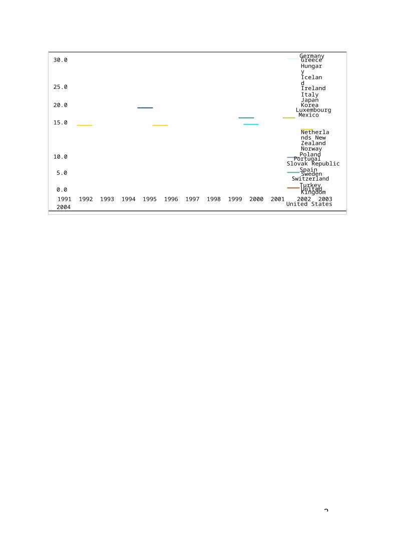
Total expenditure on pharmaceuticals (% TEH)1991 1992 1993 1994 1995 1996 1997 1998 1999 2000 2001 2002 2003 2004

AustraliaAustria Belgium CanadaCzech Republic Denmark FinlandFrance Germany Greece Hungary Iceland Ireland Italy Japan KoreaLuxembourg Mexico Netherlands New Zealand Norway Poland PortugalSlovak Republic SpainSweden Switzerland TurkeyUnited KingdomUnited States

9.5 9.9 10.4 11.0 11.2 11.5 11.7 12.0 12.6 13.5 14.0 14.29.2 9.3 11.1 12.1 12.7 12.6 12.3 12.8 13.1 13.0

15.6 16.3 17.4 17.5 16.8 16.2 16.5 11.311.8 12.4 13.0 13.1 13.8 14.0 14.8 15.2 15.5 15.9 16.2 16.7 17.0 17.718.4 21.1 19.4 24.7 25.1 25.0 24.9 22.9 23.0 22.4 21.5 22.08.0 7.9 8.5 8.8 9.1 8.9 9.0 9.0 8.7 8.8 9.2 9.8 10.0 9.49.9 10.8 12.3 13.4 14.1 14.4 14.8 14.6 15.0 15.5 15.8 16.0 16.0 16.3

17.2 17.1 17.5 17.4 17.6 17.6 18.0 18.6 19.5 20.3 20.9 18.7 18.8 18.914.7 13.2 12.9 12.7 12.8 12.9 13.4 13.5 13.6 14.2 14.5 14.6

16.3 17.0 16.6 16.1 15.7 16.1 16.2 13.9 14.4 15.0 15.1 16.2 17.1 17.427.6 26.5 28.4 28.0 25.0 26.0 25.9 28.5 27.612.3 13.0 12.4 13.1 13.4 14.0 15.1 14.8 14.3 15.1 14.4 14.7 14.5 14.811.6 11.1 10.7 10.6 10.4 10.5 10.2 10.4 10.5 10.6 10.3 11.0 11.8 12.420.8 20.8 20.2 20.3 21.1 21.3 21.5 22.0 22.6 22.4 22.6 22.5 22.1 21.422.9 22.0 22.3 21.1 22.3 21.6 20.6 18.9 18.4 18.7 18.8 18.4 18.935.0 33.3 32.3 31.3 31.4 30.2 27.7 25.8 25.1 27.8 27.6 27.9 27.6 27.415.0 12.2 12.0 11.5 12.6 12.3 11.9 11.0 11.5 10.3 9.4 8.5

18.6 19.4 19.6 21.2 21.5 20.99.6 10.5 11.0 10.9 11.0 11.0 11.0 11.2 11.4 11.7 11.7 11.5

14.1 14.2 14.9 15.8 14.8 14.5 14.47.3 7.5 9.6 8.8 9.0 9.1 9.1 8.9 8.9 9.5 9.3 9.4 9.2 9.5

28.4 30.3 29.624.3 24.7 25.6 25.2 23.6 23.8 23.8 23.4 22.4 23.0 23.3 22.6 23.2

34.0 34.0 34.0 37.3 38.519.2 19.8 20.8 21.0 21.5 21.3 21.1 21.8 22.8 22.8

8.7 9.7 10.7 11.8 12.3 13.6 12.4 13.6 13.9 13.8 13.2 13.0 12.6 12.39.8 9.4 9.7 9.8 10.0 10.0 10.3 10.2 10.5 10.7 10.6 10.3 10.5 10.4

31.6 24.3 24.813.8 14.2 14.8 15.1 15.3 15.6 15.89.0 8.7 8.5 8.5 8.9 9.3 9.7 10.3 11.1 11.7 12.0 12.3 12.4 12.3


45.0Australia Austria

40.0 BelgiumCanadaCzech Republic

35.0 DenmarkFinlandFrance

30.0 GermanyGreeceHungary Iceland25.0 IrelandItaly Japan

20.0 KoreaLuxembourg

Mexico15.0 Netherlands

New Zealand Norway

10.0 PolandPortugalSlovak Republic

5.0 SpainSwedenSwitzerland

0.0 Turkey

United Kingdom1991 1992 1993 1994 1995 1996 1997 1998 1999 2000 2001 2002 2003 2004 United States

2

alt

tinez-Gir Mar

Xavier

Qc

Economics

Healthof

inciples Pr

2-

alt

tinez-Gir Mar

Xavier

Qc

Economics

Healthof

inciples Pr

2-

Reading:

Doyle, J., 2007, Returns to Local-Area Health Care Spending: Using health stocks to patients far from home, NBER WP 13301

[http://www.nber.org/papers/w13301]

2-

alt

tinez-Gir Mar

Xavier

Qc

Economics

Healthof

inciples rP

National Bureau of Economic ResearchHTTP://WWW.NBER.ORG/

Higher Health Spending Saves Lives

"A typical comparison of a high-spending area and a low-spending one means a 50 percent difference in health care spending intensity�This disparity is associated with a 1.6 percentage-point lower mortality rate among heart emergency patients. Based on that estimate, the additional cost of a statistical life-year-saved is on the order of $50,000."

Health care spending is a major concern in the United States, amounting to over $2 trillion per year or 16 percent of GDP. These figures are expected to increase with the aging of the population and are likely to strain government budgets and private-sector profitability. And, there is controversy over exactly what we are getting for that health care spending.

Among counties or regions within the United States, there are large disparities in spending, yet health outcomes are remarkably similar. One study of Medicare data found that end-of-life spending levels -- a measure of treatment intensity that controls for the health outcome -- are 60 percent higher in high spending areas of the United States than in low spending areas. Yet there is no difference across regions in five-year mortality rates after such health events as heart attacks or hip fractures.

One difficulty that arises when comparing regions is that populations in worse health may receive greater levels of treatment. For example, at the individual level higher spending is strongly associated with higher mortality rates, because more is spent on sicker patients. At the regional level, long-term investments in capital and labor also may reflect the underlying health of the population.

In Returns to Local-Area Health Care Spending: Using Health Shocks to Patients Far From Home (NBER Working Paper No. 13301), author Joseph Doyle compares outcomes of patients who are exposed to different health care systems that were not designed for them: patients who are far from home when a health emergency strikes. These visitors vacation in areas that provide different levels of health care. They may have a health emergency in an area that spends a great deal on patients or in one that tends to spend less. By comparing similar visitors across these locations, Doyle is able to use differences in health outcomes to shed light on the returns to health care spending, at least in emergency situations.

He finds that if the medical emergency occurred in a high-spending area, the patient was significantly more likely to survive. This result comes from analyzing groups of counties with similar lodging prices that are also popular tourist destinations -- areas that are likely to be close substitutes in terms of vacations, and that provide credible variation in health care systems.

In particular, Doyle uses data from hospital discharges in the state of Florida -- one of the most frequently visited states, which also gathers a wealth of data on patient characteristics. A typical comparison of a high-spending area and a low- spending one means a 50 percent difference in health care spending intensity. Doyle finds that this disparity is associated with a 1.6 percentage-point lower mortality rate among heart emergency patients. Based on that estimate, the additional cost of a statistical life-year-saved is on the order of $50,000 -- similar to the estimate from health improvements over time, and well below the typical value of a life-year-saved of $100,000.

Doyle's results also confirm earlier findings of little relationship between spending and mortality among the populations the health care systems are designed to serve. Instead, those who have a serious health emergency far from home are exposed to different health care systems, but they are unlikely to affect the resources available in the systems.

Doyle points out that visitors choose their destinations, and if relatively healthy individuals were to choose high-spending areas, then his main results would reflect these differences. However, his estimates are robust across different types of patients, including those with various income levels, and within groups of destinations that can be characterized as close substitutes. The returns to spending are lower in places where the visitors were more likely to select the destination with the health care system in mind -- this suggests that Doyle's main results may understate the benefits of health care spending.

-- Les Picker

The Digest is not copyrighted and may be reproduced freely with appropriate attribution of source.

2-

alt

tinez-Gir Mar

Xavier

Qc

Economics

Healthof

inciples Pr

2-

alt

tinez-Gir Mar

Xavier

Qc

Economics

Healthof

inciples Pr

2

⊗

0

⊗ →

−→

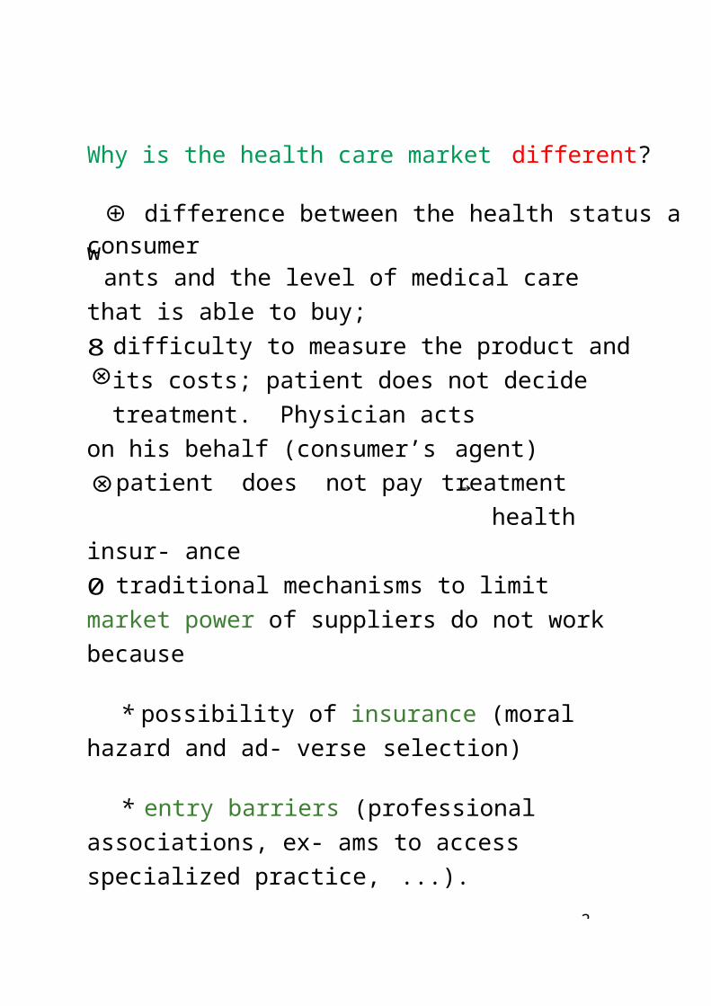
Why is the health care market different?

w⊕ difference between the health status a consumerants and the level of medical care that is able to

buy;difficulty to measure the product and its costs; patient does not decide treatment. Physician acts

on his behalf (consumer’s agent)patient does not pay treatment health insur-

ancetraditional mechanisms to limit market power of

suppliers do not work because

* possibility of insurance (moral hazard and adverse selection)

* entry barriers (professional associations, exams to access specialized practice, ...).

Also, external factors contribute:

† population aging,

‡ technological development.

Consequence: MARKET INTERVENTION. [ no guarantee of proper behavior!!]

8

2

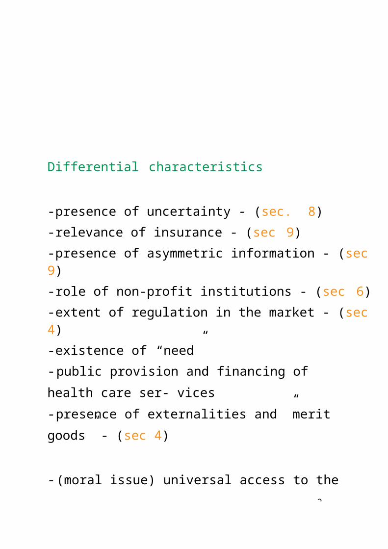
Differential characteristics

- presence of uncertainty - (sec. 8)- relevance of insurance - (sec 9)- presence of asymmetric information - (sec 9)- role of non-profit institutions - (sec 6)- extent of regulation in the market - (sec 4)- existence of “need”- public provision and financing of health care services- presence of externalities and ”merit goods” - (sec 4)

- (moral issue) universal access to the health care system

2

→

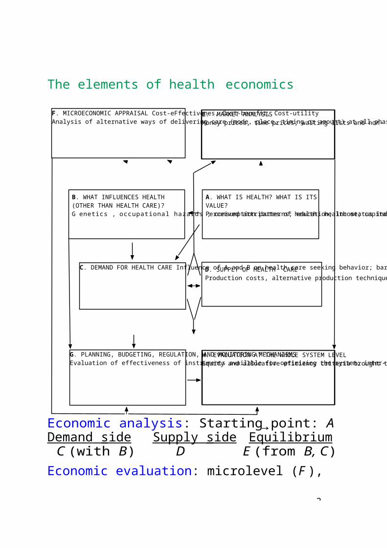
B. WHAT INFLUENCES HEALTH(OTHER THAN HEALTH CARE)?G enetics , occupational hazards ; consumption patterns; education; income; capital (human and physical), family background, etc.

A. WHAT IS HEALTH? WHAT IS ITSVALUE?Perceived attributes of health; health status indices; value of life; utility scaling oh health.

D. SUPPLY OF HEALTH CAREProduction costs, alternative production techniques, input substitution; markets for inputs; remuneration methods and incentives; forprofit and nonprofit organizations.

C. DEMAND FOR HEALTH CARE Influence of A and B on health care seeking behavior; barriers to care seeking; agency relationship; need; altruism; insurance; demand for care and its effects.

G. PLANNING, BUDGETING, REGULATION, AND MONITORING MECHANISMSEvaluation of effectiveness of instruments available for optimizing the system; inter- play of budgeting, manpower allocations, regulation, and their incentive structures.

F. MICROECONOMIC APPRAISAL Cost-eFfectivenes, Cost-benefit, Cost-utilityAnalysis of alternative ways of delivering care (mode, place, timing or amount) at all phases (detection, diagnsis, treatment, etc.)

E. MARKET ANALYSISMoney prices, time prices; waiting lists and non- price rationing systems as equilibrating mechanisms and their differential effects in markets for physician and hospital services.

H. EVALUATION AT THE WHOLE SYSTEM LEVELEquity and allocative eficiency criteria brought to bear on E and F; inter-regional and international comparisons of performance; financing methods.

The elements of health economics

Economic analysis: Starting point: ADemand side Supply side Equilibrium

C (with B) D E (from B, C)Economic evaluation: microlevel (F ), macrolevel (G) Policy analysis: H

3

tinez-Gir Mar

Xavier

Qc

Economics

Healthof

inciples Pr

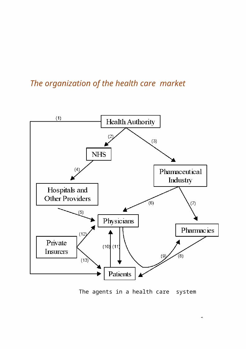
The organization of the health care market

The agents in a health care system

3-

M

artinez

Xavier

Qc

Economics

Healthof

-G

Structure of the health care system

Private provision with and without insurance

3-

Qc

Economics

Healthof

nciples ri

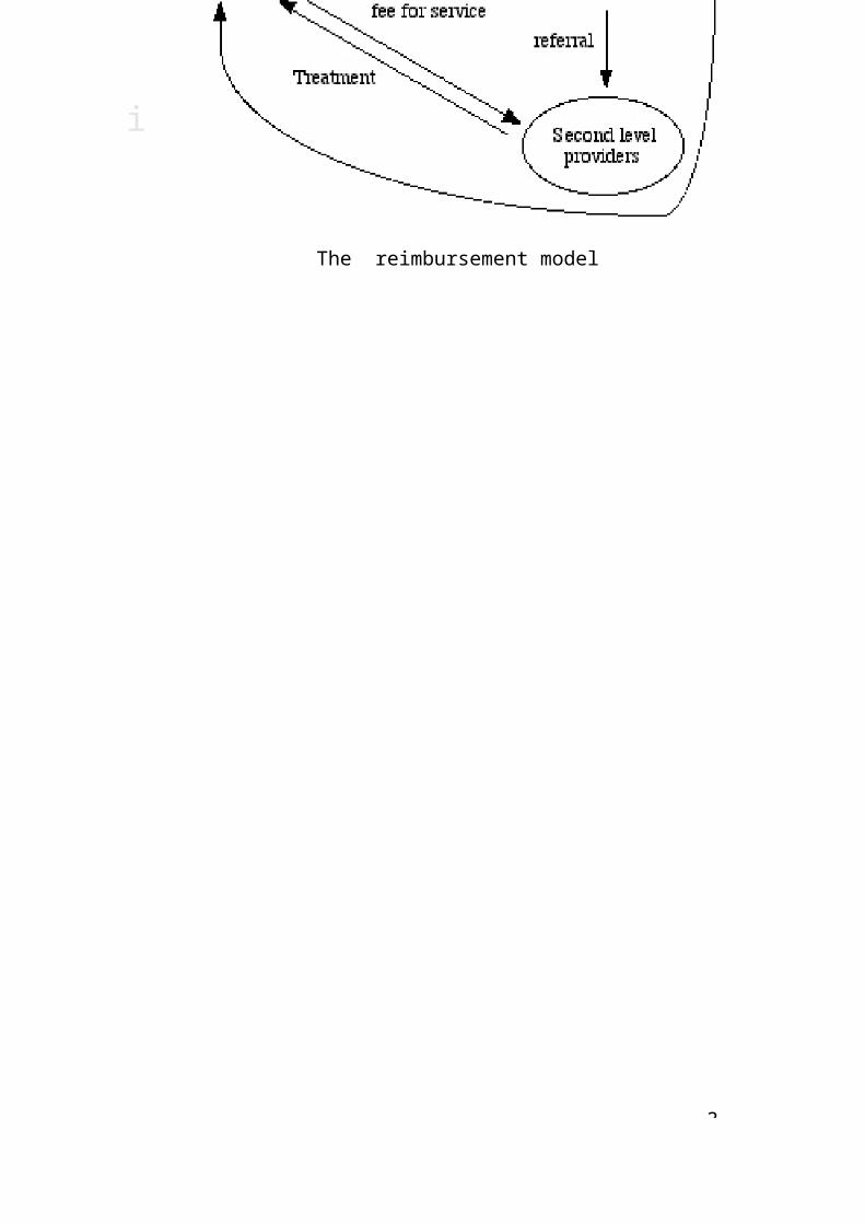
The reimbursement model

Public version (France) and private version (UK, The Netherlands).Separation between providers and 3PP.Patient advances payment and is reimbursed (par- tially or totally) by 3PP .

The reimbursement model

3

XaQc

Economics

Healthof

inciples rP

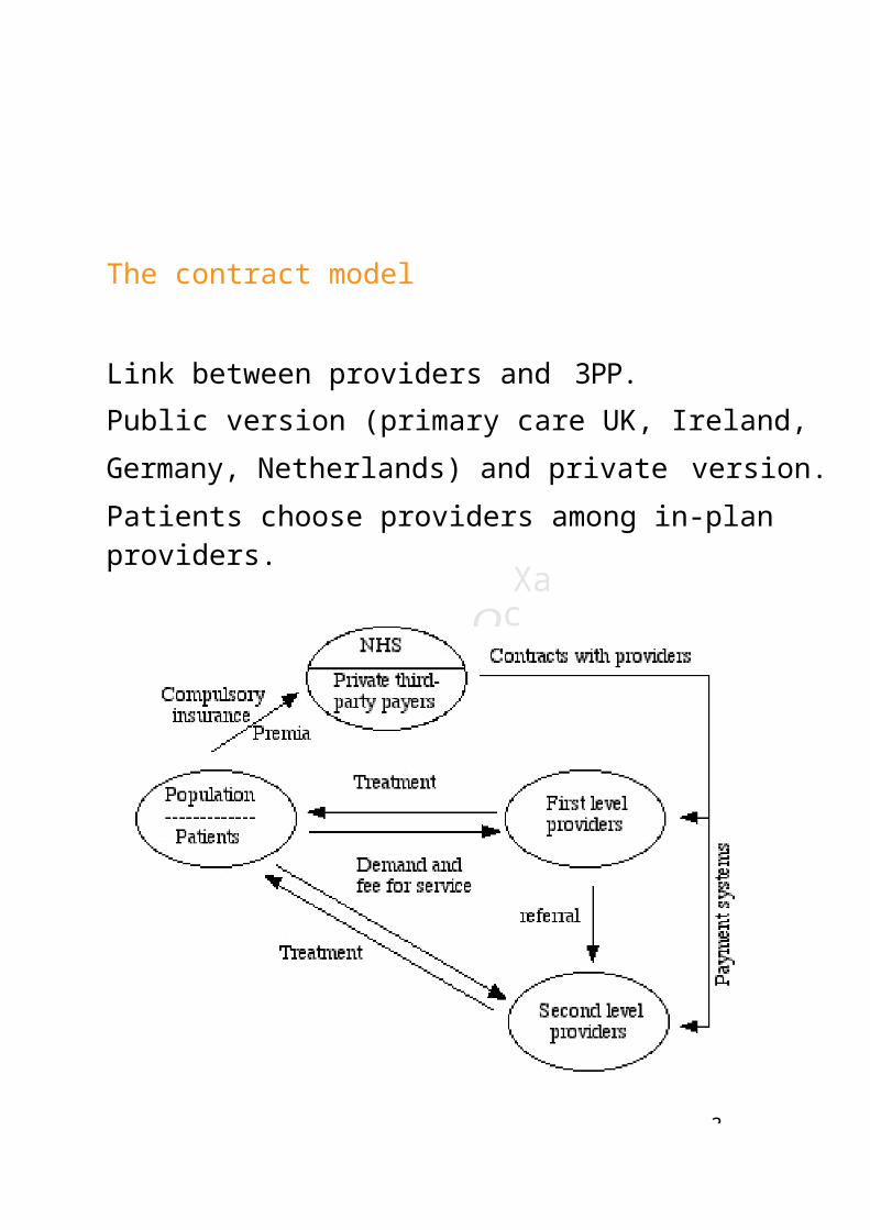
The contract model

Link between providers and 3PP.Public version (primary care UK, Ireland, Germany, Netherlands) and private version.Patients choose providers among in-plan providers.

The contract model

3-

XaQc

Economics

Healthof

inciples rP

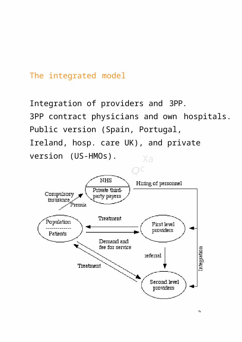
The integrated model

Integration of providers and 3PP.3PP contract physicians and own hospitals.Public version (Spain, Portugal, Ireland, hosp. care UK), and private version (US-HMOs).

The integrated model

4

alt

tinez-Gir Mar

Xavier

Qc

The actors of the health care market

- Market of insurers (3PP): Private vs Public

- Market of hospital services: Entry barriers, con- centration, Ecs. of scale, Regulation

- Market of physician services: Supplier-induced demand, Competitiveness, Costs and quality

- Also Regulation: reimbursement systems to providers

4-

Costs

Funds available

Flows of resources in industrial economics

Gross Revenues

Retained earnings

Stock market valuation

External funds

Prices / production

Markets

Demand SupplyProfits

Acquisitions Advertising Marketing

R&D Capital investment Dividends

4-

Gross Revenues

Costs

Retained earnings

Stock market valuationFunds available External funds

Prices / production

Markets

Demand Supply

Financial flows in industrial economics

- Generation of resources

- Distribution of profits

Profits


R&D Capital investment Dividends

4

Economic

s Healthof

Funds available

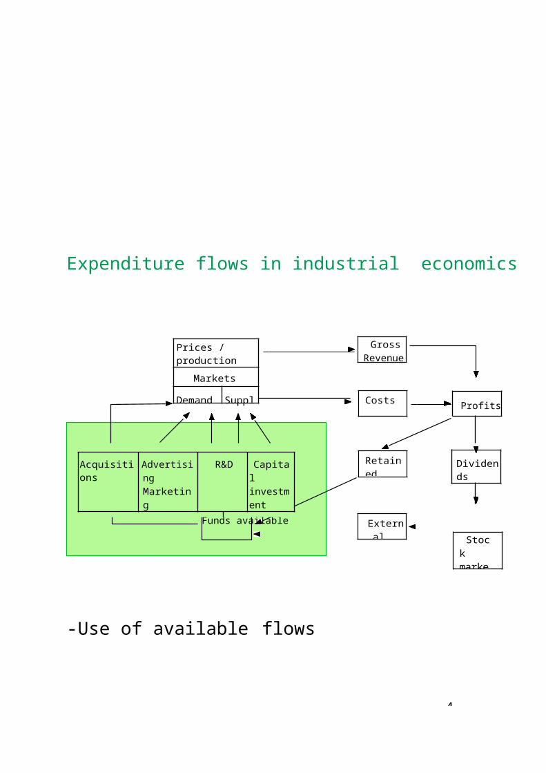
Expenditure flows in industrial economics

- Use of available flows


R&D Capital investment

External funds

Gross Revenues

Costs

Retained earnings


Prices / production

Markets

Demand SupplyProfits

Dividends

4-

Xavier

Qc

Gross Revenues

Costs Profits

Funds available

Market flows in industrial economics

Prices / production

Markets

Demand Supply

- Generation of profits

DividendsAcquisitions Advertising Marketing

R&D Capital investment

Retained earnings


External funds

5

Qc

Economics

Healthof

inciples Pr

2. The agents of the economy

Population/ Patients

(Demand)

5-

Ma Xa

vier

Qc

Economics

Healthf

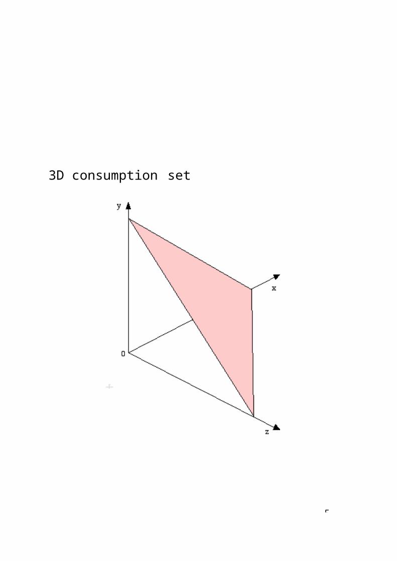
3D consumption set

5-

Health of

inciples r

x y

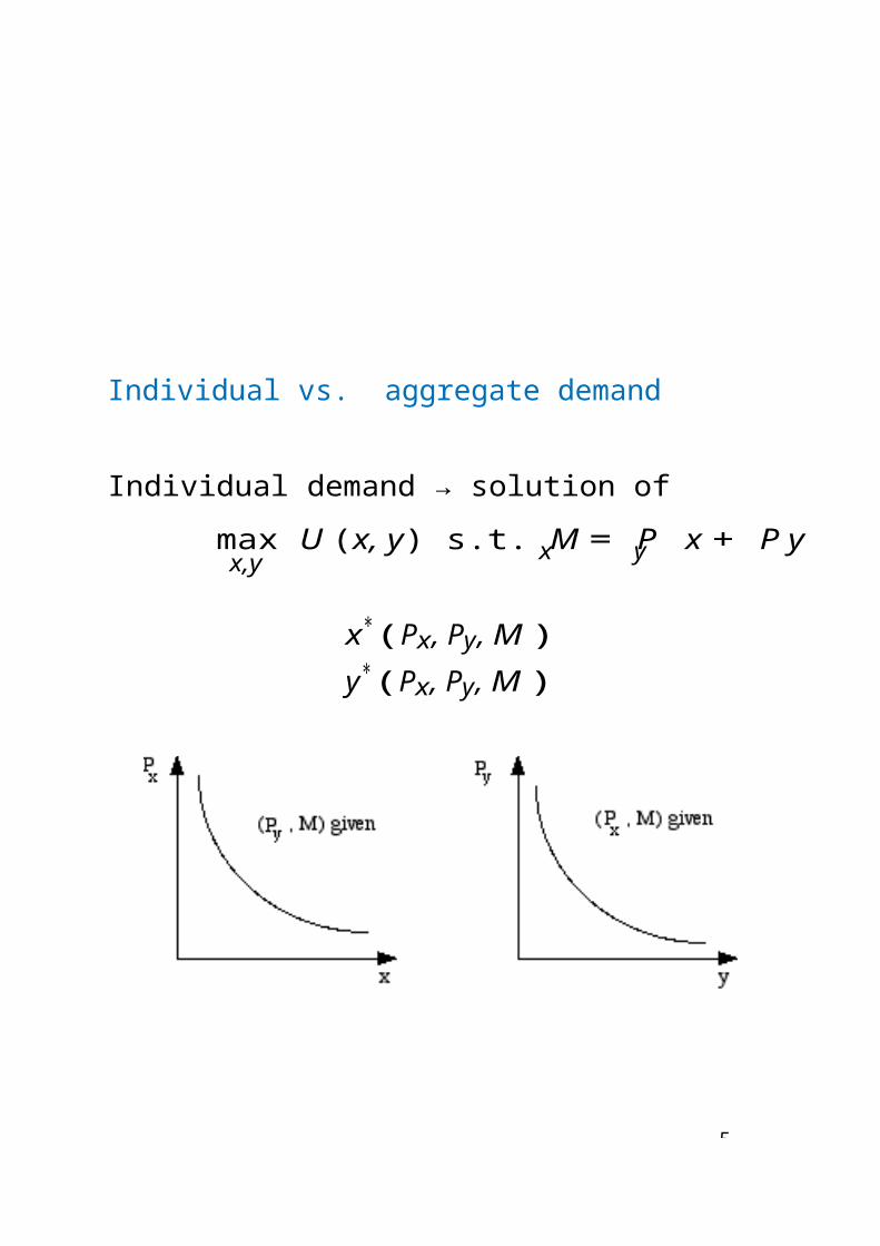
Individual vs. aggregate demand

Individual demand → solution of

max U (x, y) s.t. M = P x + P yx,y

x∗(Px, Py, M )y∗(Px, Py, M )

5

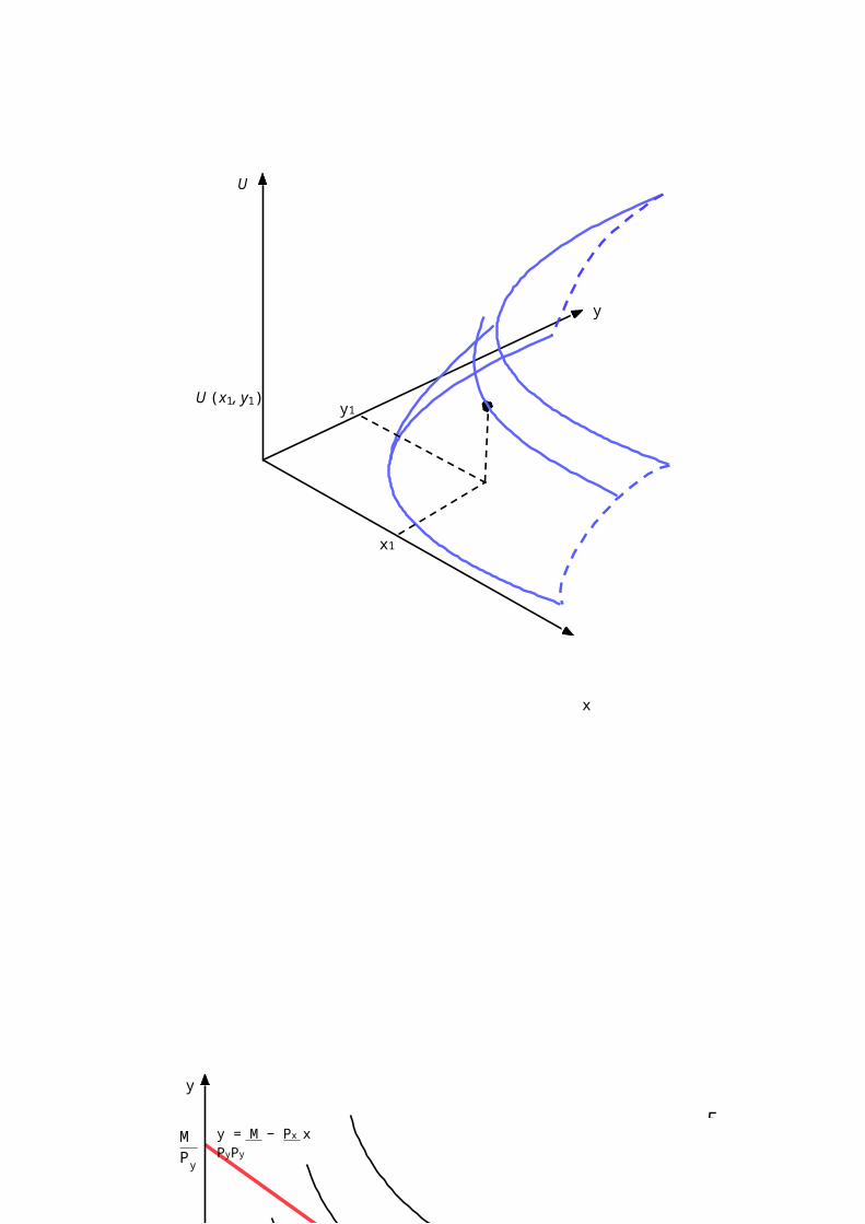
y

y1

x1

y

MP

y = M − Px xPyPy

y

y∗u3

u2Du

u1

U

U (x1, y1)

x

x∗ M xPx

5-

Qc

Economics

Healthof

inciples Pr

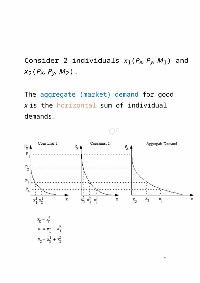
Consider 2 individuals x1(Px, Py, M1) andx2(Px, Py, M2).

The aggregate (market) demand for good x is the horizontal sum of individual demands.

5-

Economic

s Healthof

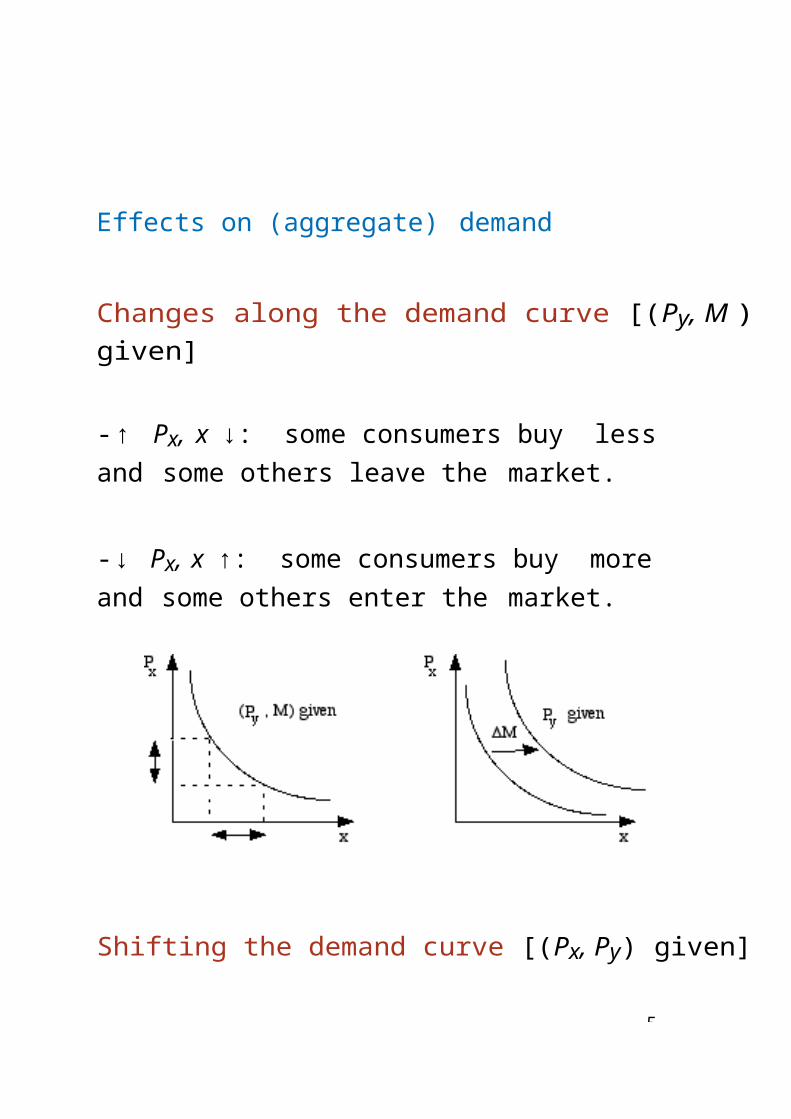
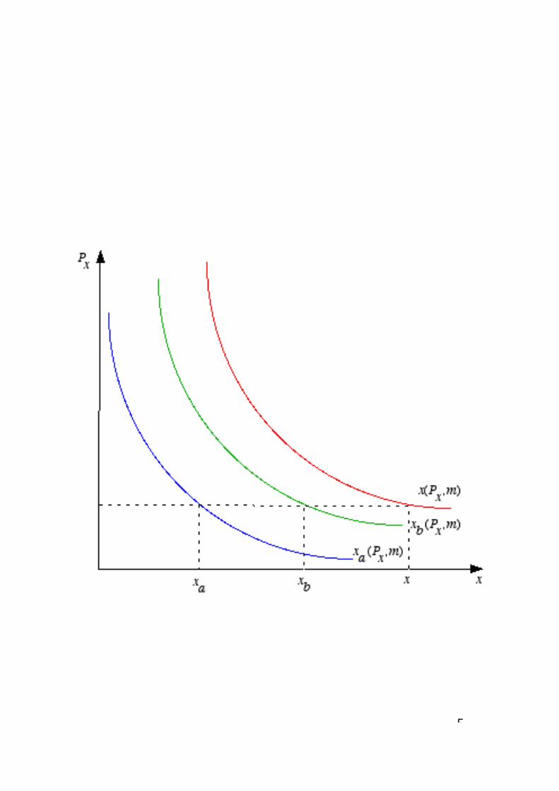
Effects on (aggregate) demand

Changes along the demand curve [(Py, M ) given]

- ↑ Px, x ↓: some consumers buy less and some others leave the market.

- ↓ Px, x ↑: some consumers buy more and some others enter the market.

Shifting the demand curve [(Px, Py) given]

- ↑ M −→ increase demand x and y: demand curve moves outwards.

5

↑

M given Py

M given Py

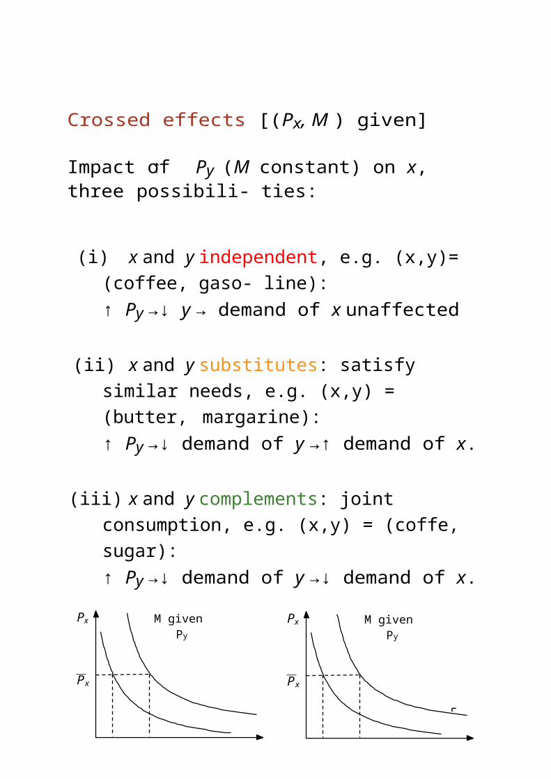
Crossed effects [(Px, M ) given]

Impact of Py (M constant) on x, three possibilities:

(i) x and y independent, e.g. (x,y)= (coffee, gasoline):↑ Py →↓ y → demand of x unaffected

(ii) x and y substitutes: satisfy similar needs, e.g. (x,y) = (butter, margarine):↑ Py →↓ demand of y →↑ demand of x.

(iii) x and y complements: joint consumption, e.g. (x,y) = (coffe, sugar):↑ Py →↓ demand of y →↓ demand of x.

Px Px

Px Px

x1 x2 x2 x1

(x, y) substitutes (x, y) complements

5-

1

Elasticity

How to measure the impact of ∆Px on

x? Method 1: Direct and simple

∆x∆Px

Problem: dependent on units

EURO US $Px

x Pxx

6 10 8 10

12 5 16 5

∆ x 1

1

1

= − 5 = −0.83

∆Px 1

1EU R 6 ∆ x

∆1

1$

5-

= − 5 8

= −0.625

5-

x

1

1%∆P

11

=

11 ∆Px

11

=Px

1

1∆Px1

1

2

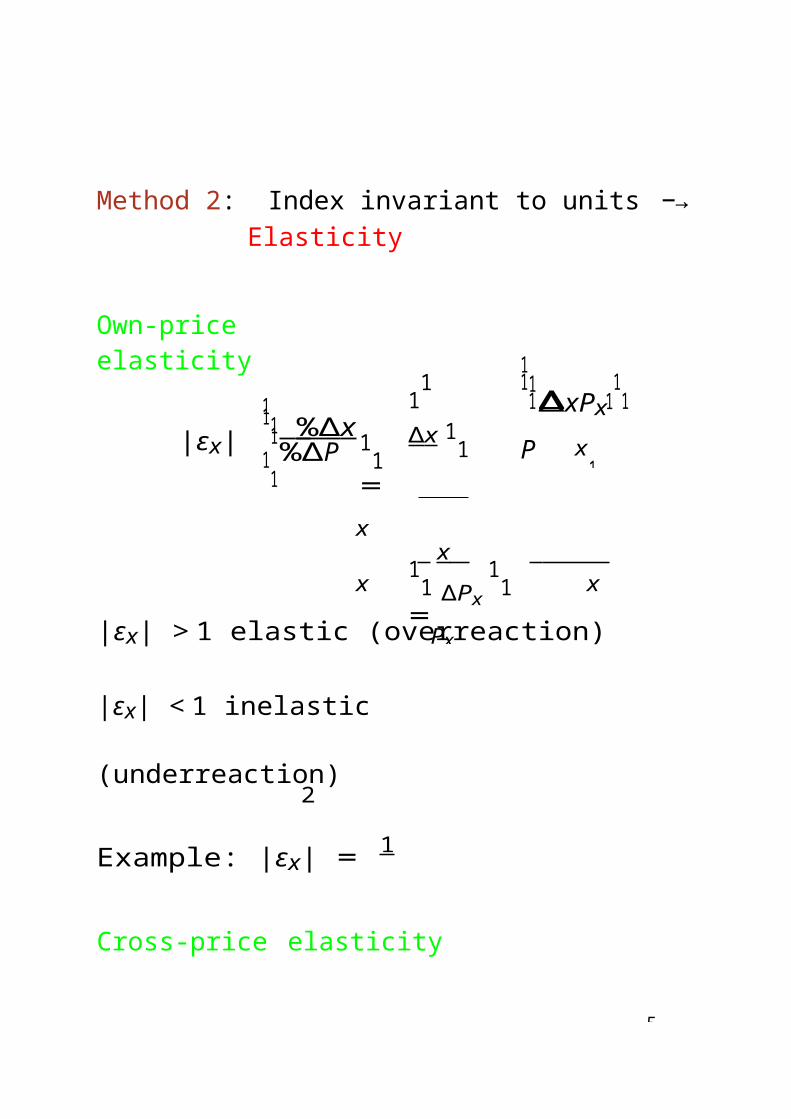
Method 2: Index invariant to units −→Elasticity

Own-price elasticity1

1 %∆ x 1

1

x

11 ∆x

11

11∆xPx

11

x x

|εx| > 1 elastic (overreaction)

|εx| < 1 inelastic

(underreaction) Example: |εx|

= 1

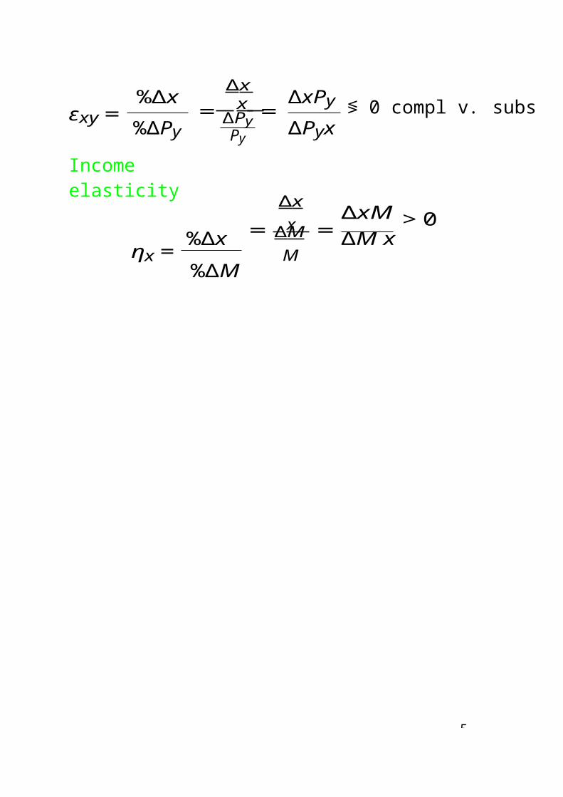
Cross-price elasticity

εxy =

%∆x%∆Py

∆ x

= x =∆PyPy

∆xPy∆Pyx

≶ 0 compl v. subs

Income elasticity %∆x ηx =

%∆M

x

|εx| =

5-

= x ∆x ∆xM∆M ∆M x

> 0

M

=

5

≥ x y

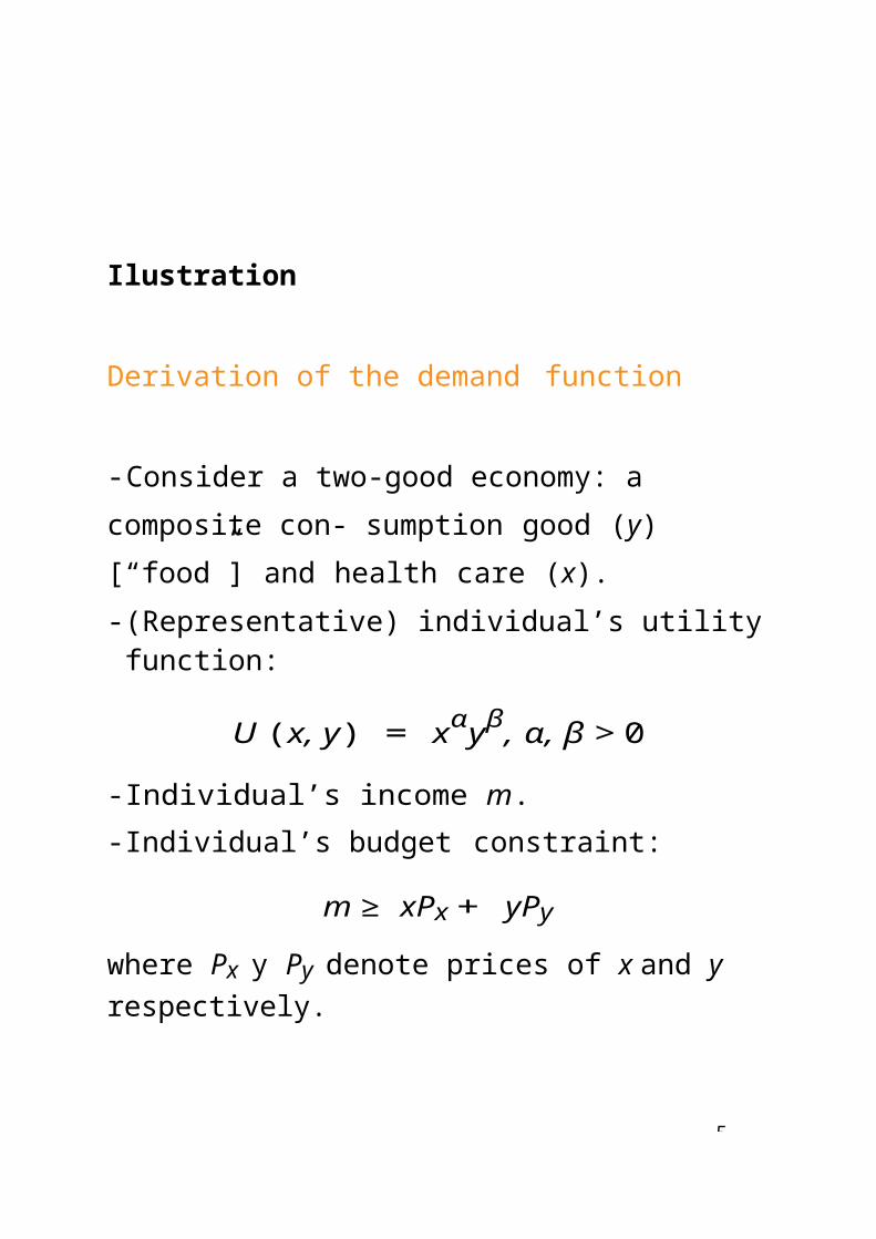
Ilustration

Derivation of the demand function

- Consider a two-good economy: a composite consumption good (y) [“food”] and health care (x).- (Representative) individual’s utility function:

U (x, y) = xαyβ, α, β > 0

- Individual’s income m.- Individual’s budget constraint:

m ≥ xPx + yPy

where Px y Py denote prices of x and y respectively.

- Individual’s problem:Select a bundle (x, y) to maximize utility given (Px, Py; m):

max xαyβ s.t. m xP + yPx,y

5

x,y

−∂L

−∂L

Solution:

max L(x, y) = xαyβ + λ(m − xPx − yPy)

First order conditions,

= αxα−1yβ λPx = 0 (1)∂x

= βyβ−1xα λPy = 0 (2)∂y

∂λ = m − xPx + yPy = 0 (3)

From (1) and (2),

That is,

αy =

Px βx Py

y = βx

Px(4)

α Py

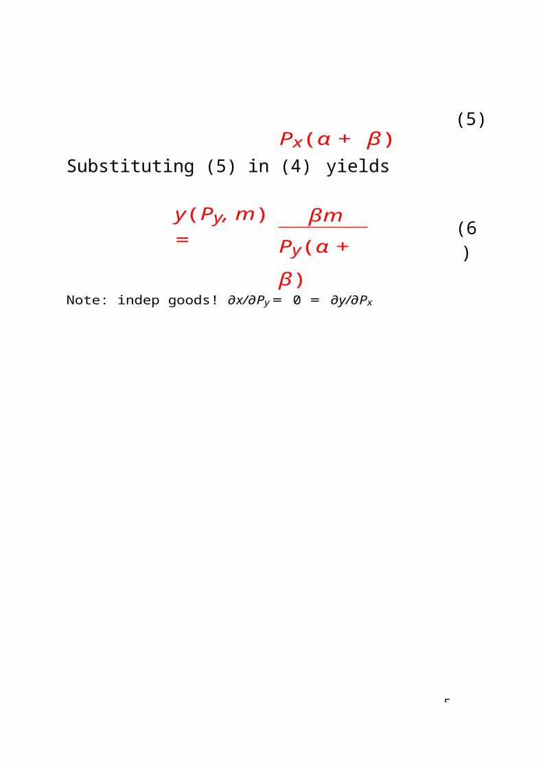
Substituting (4) in (3) yieldsx(Px, m) =

αm(5)

Px(α + β)Substituting (5) in (4) yields

y(Py, m) =

βm Py(α + β)

∂L

5

(6)Note: indep goods! ∂x/∂Py = 0 = ∂y/∂Px

5

Example Society with two consumers a and b and two goods x and y.

1 2Ua(xa, ya) = x3 y 3a a2 1

Ub(xb, yb) = x3 y 3b b

Individual demands:

xa(Px, m) =m

3Px

2mya(Py, m) =

3Py2m

xb(Px, m) = 3Pxm

yb(Py, m) = 3P

Market demands:y

x(Px, m) = m

Px y(Py, m) = m

Py

5

tinez-Gir Mar

Xavier

Qc

Economics

Healthof

inciples

5-

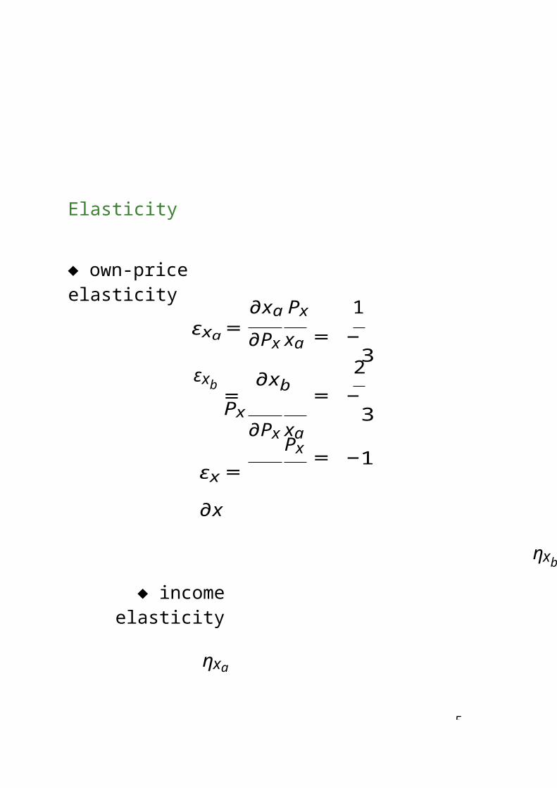
Elasticity

♦ own-price elasticity

∂xa Px 1εxa = ∂Px xa = −

3εxb

= ∂xb

Px∂Px xa

2= −

3

εx =∂x Px = −1

♦ income elasticity

ηxa

ηxb

∂Px xa

= ∂xa m

= 1∂m xa

= ∂xb m

= 1∂m xa

ηx = ∂x m = 1∂m xa

5-

tinez-Gir Mar

Xavier

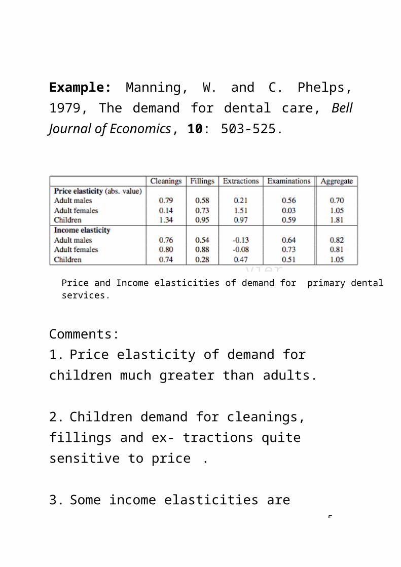
Example: Manning, W. and C. Phelps, 1979, The demand for dental care, Bell Journal of Economics, 10: 503-525.

Price and Income elasticities of demand for primary dental services.

Comments:1. Price elasticity of demand for children much greater than adults.

2. Children demand for cleanings, fillings and extractions quite sensitive to price .

3. Some income elasticities are substantial in cleanings and examinations.

4. Negative income elasticity for extractions in adults: “poor people’s dentistry”.

5-

Readings:

Manning, W. and C. Phelps, 1979, The demand for dental care, Bell Journal of Economics, 10: 503- 525.

[http://ideas.repec.org/a/rje/bellje/v10y1979iautumnp503-525.html]

AIHW, 2003, Demand for dental care, AIHW Dental Statistics and Research Unit Research Report No. 8.

[http://arcpoh.adelaide.edu.au/publications/report/research/]

Note: Usually dental care is not covered by health insurance. Demand for dental care is thus sensitive to price variations.

6

Possibilities Technology

Supply Feasible production set

C(x) F V (x)AC(x) C(x)xMC(x) C(x)

x

Producers (Suppliers).

Production functionTechnological costs

- Total- Average- Marginal

Opportunity costs. EfficiencyPPF

input 1Production possibility frontier

Opportunity set

input 2

output

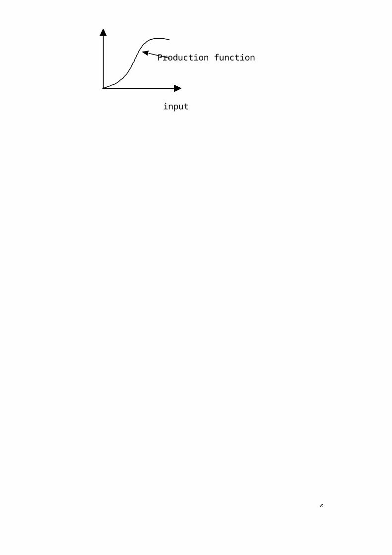
Production function

input

PRODUCERS What and how much to produce

Econ

omic

cos

ts

6-

Production function

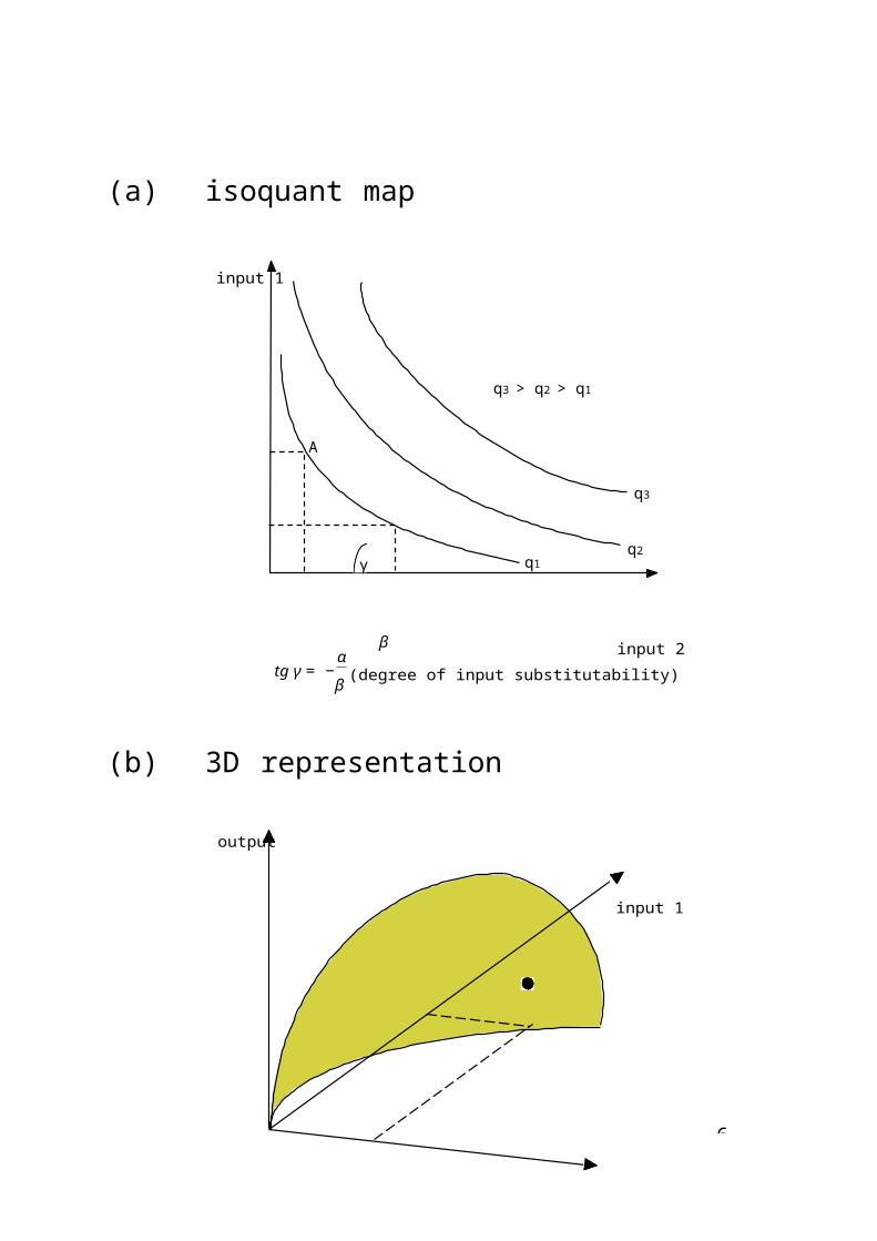
♠ relation between output and inputs: output = f(inputs).→ engineering approach to production activity.bread=f(flower, water, salt, labor, ...) surgery=f(surgery room, blood, anesthesia, nurse, surgeon, ...)e.g. q = f (K, L)

♠ Def.: represents the maximum amount of output that can be obtained from a given combination of inputs. (conveys efficiency)

♠ Graphical representation (1 output, 2 inputs):

(a) isoquant map → degree of substitutability of inputs.

(b) 3D

(c) Production possibility frontier (multiproduct)

6-

q3 > q2 > q1

A

q3

q2γ q1

(a) isoquant map

input 1

αβ input 2

tg γ = −β (degree of input substitutability)

(b) 3D representation

output

input 1

0

input 2

6

5045

B

25A

16 C

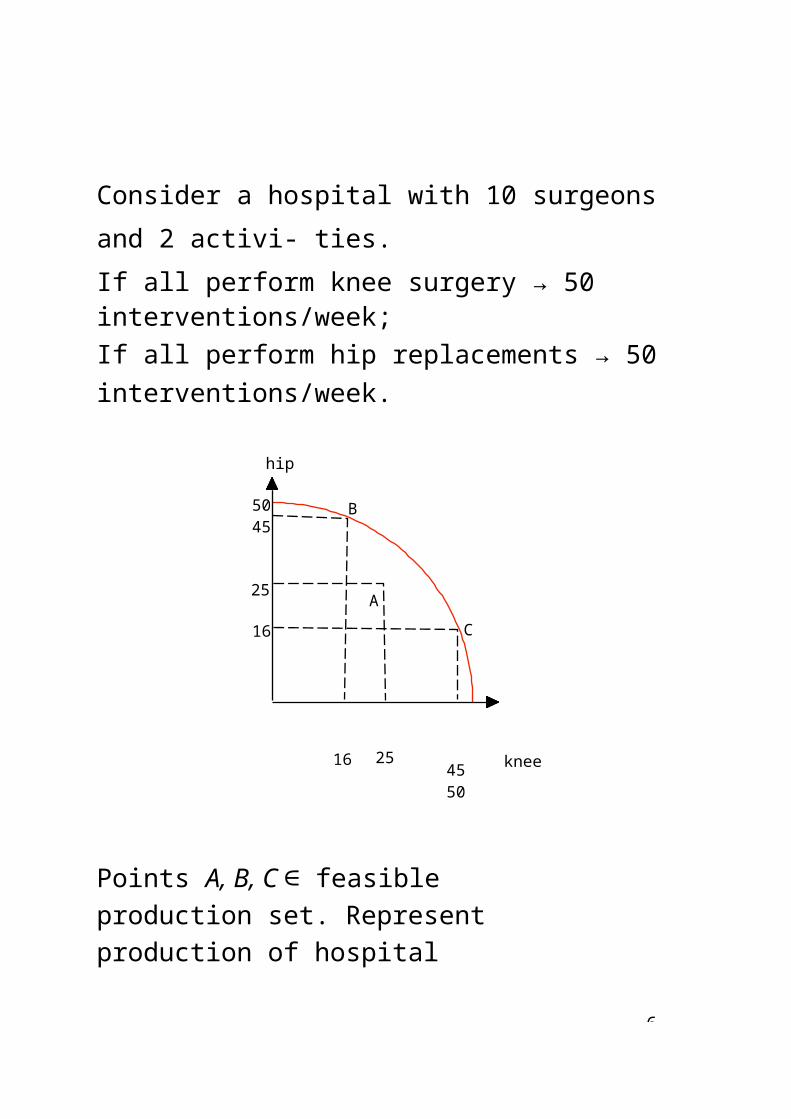
Consider a hospital with 10 surgeons and 2 activities.If all perform knee surgery → 50 interventions/week;If all perform hip replacements → 50 interventions/week.

hip

16 2545 50 knee

Points A, B, C ∈ feasible production set. Represent production of hospital (supply). Points B, C ∈ FPP.

Production possibility frontier:Set of all the maximum combinations of operations the hospital can achieve given the quantity and productivity of resources available.

6-

Efficiency.

An allocation of resources is efficient if it is impos- sible to change that allocation to make a consumer better off (perform one additional intervention) without making anybody else worse off (reducing number of operations).

Efficiency refers to allocations of resources yielding the maximum possible output, i.e. allocations on PPF.

Hence, allocation A is not efficient, while allocationsB, C are efficient.

From a social point of view, there is interest in moving from A to B (or C). The hospital is able to increase its output with the same inputs.

6-

Efficacy.

Potential benefit of a technology. Probability that an individual benefits from the application of a (health) technology to solve a particular (health) problem, under ideal conditions of application.

Effectiveness.

Probability that an individual benefits from the application of a (health) technology to solve a particular (health) problem, under real conditions of application.

Examples:

Highly effective treatments: vaccinations, heart surgery, diabetes, influenza, renal insufficiency, ...

Clinical interventions of known efficacy explain 5 of the years won in life expectancy at birth.

6

Efficacy vs Effectiveness

In general, efficacy or ideal use or perfect use is the ability to produce a specifically desired effect. For example, an efficacious vaccine has the ability to prevent or cure a specific illness. In medicine a distinction is often drawn between efficacy and effectiveness or typical use. Whereas efficacy may be shown in clinical trials, effectiveness is demon- strated in practice.

The distinction between efficacy and effectiveness is important because doctors and patients often do not follow best practice in using a treatment. For instance, a patient using oral con- traceptive pills to prevent pregnancy may sometimes forget to take a pill at the prescribed time; thus, while the perfect-use failure rate for this form of conception in the first year of use is just 0.3%, the typical-use failure rate is 8%.

6-

Illustration

* Clinical essay: efficacy of drug 1=75%.* ∃ drug 2, same price and efficacy = 70%

more effective to select drug 1 and reject drug 2?

YES, with this information.

Additional INFO

◆ both drugs are correctly prescribed to 75% of patients◆ drug 1: 50% of patients follow treatment correctly (shots)◆ drug 2: 70% of patients follow treatment correctly (pills)

Effectiveness of drugs:

E1 = 0.75 × 0.75 × 0.5 = 0.28125E2 = 0.7 × 0.75 × 0.7 = 0.3675

Conclusion: select drug 2.

6-

q¯

∂q

r r

Cost function

Cost function shows relationship between output and cost. → economic approach to production activity.

Def.: minimum possible cost of production of a given volume of output (q¯). (conveys efficiency)CT (q¯) = minK,L rK + wL s.t.q = f (K, L)→ K(q¯), L(q¯)

Example: Let,q represent physician office visits,L represent labor input (with price w = 1 e),K represent capital input (with price r = 1.2

e). We are assuming competitive markets!

Short run vs. long run: fixed costs.Total cost: T C(q¯) = rK(q¯) + wL(q¯) =

1.2K(q¯) + L(q¯)Average cost: AC(q¯) = T C (q¯)

Marginal cost: M C(q¯) = ∂ T C (q¯)

Representation: Isocost map → K = T C − w L

6

→

→

K

TC3

rTC3 > TC2 > TC1

TC2

r

TC1

rK = TC 3 w

r−L

r

TC1 TC2 TC3

TC1

wTC2

wTC 3 Lw

To derive the total cost function, combine isocost map and isoquant map:

- To produce q = 100 (i.e. 100 visits of patients) given the prices w and r, the physician minimizes cost by contracting 20 units of labor and 25 of capital. This yields a total cost of T C(100) = (1.2)25+ 20 = 50 e.

- To producte q = 150, T C(150) = (1.2)40 + 30 = 78 e

- To producte q = 200, T C(200) = (1.2)50 + 45 = 105 e

6

C

B

A q = 200

q = 150

q = 100

TC(q)

C

B

A

TC(q)

δ

γ

MC(q)AC(q)

K TC

105

50 78

40 50

25

20 30 45 L 100 150 200 q

TC ACMC

TC(q˜)

q˜ q q

TC(q˜)AC(q˜) = tg γ =;

q˜

MC(q˜) = tg δ

6

∂

⇔

−

Remark 1: decreasing (long run) AC implies a range of values of q such that M C(q) < AC(q).

∂AC(q)

= ∂q

T C ( q ) q =∂q

M C(q)q T C(q)

q2 =

M C(q)

q

−

AC(q)< 0 M C(q) < AC(q)

q

Remark 2: let qˆ be such that AC(qˆ) is minimum.Then, AC(qˆ) = M C(qˆ).

If AC(qˆ) is minimum means derivative = 0. Thus,T C ( q )

∂ A C ( q ) 1

11 =

∂ q1

11 =

M C ( q ) q − T C ( q ) 1

11 =∂q

1qˆ

∂q

1qˆ

q2 1qˆ

6

1

1

M C ( q )

11

1

AC ( q ) − 1 = 0 ⇔ M C(qˆ) = AC(qˆ)

q 1qˆ q 1

qˆ

6

Economies of scale

Economies (diseconomies) of scale characterizes a production process in which an increase in the level of production causes a decrease (increase) in the long run average cost of each unit.

AC

AC(q)

optimal size of hospital q

6-

Economies of scope

Economies of scope may appear in multiproduct firms. Scope economies refer to changes in average costs induced by changes in the mix of output between two or more products. In other words, they refer to the potential cost savings from joint production.

Consider a community with two hospitals. One specialized in pediatric care (q1), the other specialized in cancer care (q2). May it be worth to merge both activities in a single hospital?

Scope economies arise if

T C(q1, q2) < T C(q1) + T C(q2)

That is, the joint production of pediatric and cancer care allows for savings in the hospital’s management structure, administration systems, management of hospital capacity, nurses, and non-sanitary personnel, etc.

6-

Opportunity cost.

The concept of opportunity cost is defined as the benefit given up by not choosing an alternative allocation.

Assume a shift from B to C (page 6b). Consequences?

- 29 additional heart surgery interventions- 29 less hip replacements.

The opportunity cost of moving from B to C is the reduction in hip replacements due to the increase in heart operations.

The opportunity cost is an economic concept (not in accountancy).

6-

How does society chooses among feasible allocations? VOTING mechanism.

Criteria to be used:

- Efficiency: Select only efficient allocations (rule out allocation A)

- Equity. [Normative criterion] Select allocations meet- ing society’s requirement for justice.→ people’s valuese.g. social justice is behind the set-up of a NHS.

*Horizontal and Vertical equity.

• Horizontal equity: equal treatment of equal need. D 2 individuals with same illness and severity should receive same treatment.

• Vertical equity: unequal treatment of unequal need. D more treatment for patients with serious conditions than for those with minor affections.D passing the financing of health care to ability to pay (progressive income tax).

6-

Technical progress and its diffusion

Technical progress: Defs.:

(a) produce “old” goods less costly, or produce “new” goods.

(b) Ability to produce at a lower cost given a quality level.

Diffusion: who adopts a new tech, and why.

2 principles:- profit principle: physicians more likely to adopt anew surgical technique if it is expected to increase their revenue stream by enhancing their prestige and/or by improves well-being of patients. [if present valueof future profits due to innovation > 0.]- information principle: role of friends, colleagues, journals, and conferences at informing and encour- aging the adoption decision.

Trade-off:- waiting may give rivals a competitive advantage;- waiting allows for learning from others’ experience.

6-

Pt = 1+ e−(a+bt)K

(Classic) Pattern of diffusion

- Slow at the beginning;

- Then at an increasing rate;

- Then at a decreasing rate asymptotically reaching its limit K.

% adopters

K

time

(a, b) parameters to be estimated.

6

q

w given

Individual vs. aggregate supply

Individual supply → solution of

max Π(q) = qPq − C(q)

That is, (w input price vector)

q∗(Pq, w) → market structure?

Pq

q

NOTE: Pq vs. P (q).

6

q q q

Consider 2 firms q1(Pq, w) and q2(Pq, w).The aggregate (market) supply for good q is the horizontal sum of individual supplies.

Firm 1

Pq

P1

P2

Firm 2

Pq

Aggregate SupplyPq

P3

P4

1 1 q 2 21 2 1 2 q1 q2 q

q1 = q1 + q2

1 1q2 = q1 + q2

2 2

q q

6

Pq Pq

M given

q

w Tech

Effects on supply

Changes along the supply curve

- ↑ Pq, q ↑: some firms produce more and some others enter the market.

- ↓ Pq, q ↓: some firms produce less and some others leave the market.

Pq

q q

Shifting the supply curve

- ↑ w, (Pq constant), same production level is more expensive −→↓ production: supply moves inwards.

- R&D −→ more efficient technology −→ same production level is cheaper −→↑ production: supply moves outwards

6-

q

−

Illustration

Consider a firm (hospital) with a production function of health services q(l) = lδ, where l denote working hours and q health services.

The associated cost function C(w, q) = wl(q) wherel(q) = q1/δ, that is,

1C(q, w) = wq δ

The (competitive) profit function is

Π(q) = qPq − C(q)

The problem of the hospital is to determine the level of q to maximize profits. Formally,

1

max qPq − wq δ (7)

First order condition:∂ Π

= P

1 1 − δ − wq = 0.

∂qq

δδ

Thus, the supply function of the hospital is

q(Pq, w) =

(δ P q\

1 δ

δ

6-

w

6

\

P

(

Example Society with 2 (competitive) firms 1 and 2and a good q.

q1(l) =

l1/3 q2(l) = l1/2

Individual supply functions:1

q1(Pq, w) =Pq 2

3w

q2(Pq, w) = Pq

2wAggregate supply:

( P \1P 2 w

1/2 + 3 wP

q(Pq, w) =

Elasticities

q 2 +

q= 3w 2w

q q

2w(3w)1/2

εq1

εq2

= ∂q1 Pq

= 1

∂Pq q1 2

= ∂q2 Pq

= 1∂Pq q2

6-

Pq

q1(Pq, w)

q2(Pq, w)

q(Pq, w)

q

7

Insurers

Private vs Public health care systems

Private market for health insurance

- adjustment of premia to the individual risk: only weak solidarity

- Efficiency

* consumers can choose among a menu of policies

*insurers have incentives to control expenses

- Equity

* some individuals may not be insured (adverse selection problem)

* different treatment of good and bad risks

7-

Readings:

- Setting priorities:Hitchen, L., 2006, Bid to cut waiting lists has pushed safety down NHS agenda, BMJ 332(7537), Febru- ary 11: 324.

- Equity:Deemong, C., and J. Keen, 2004, Choice and equity: lessons from long term care, BMJ 328(7453), June 12: 1389-1390.

7-

→

Public centralized system for health insurance

- compulsory insurance financed through taxes and/or employer/employee contributions

- government regulation of the health care sector

- Efficiency

* limited choice for population

* spending control through government policies

- Equity

* universal coverage

* solidarity between good and bad risks

* other aspects of equity:

- equity of finance (cost-sharing by income; indiv. election insurance public/private) vs. equity of access (= treatment for = need; universal access) Deeming and Keen (2004).

- health care insurance → see ch. 7

8

3. The market and the health care market

“Place” where consumers and producers interact (i.e. exchange goods).

What goods compose a market? → demand oriented vs supply oriented

Demand oriented: set of products with high crossed elasticities among them and low wrt other goods.

Examples(a) crossed elasticity between 95 octane and 98 octane gasoline is high. They are close substitutes. They belong to the same market.(b) crossed elasticity between consumption of gasoline and mineral water is low. They are independent goods. They belong to different markets.

PROBLEM: ambiguity of high/low enough crossed elasticity.

8-

−→

Supply oriented:

- Europe NACE (General Industrial Classification of Economic Activities [Nomenclature statistique desActivite´s ećonomiques dans la Communaute´ Europeénne]),

- Spain CNAE (Clasificacioń Nacional de Actividades Econo´micas)

- US NAICS (North American Industry Classification System)

PROBLEM: codes assigned according to techno- logically oriented criteria. May be misleading, e.g. elaboration of wine and champagne have different codes, but often grouped in the same market (high crossed demand elasticity).

Imperative assumption in the study of a market: Rational behavior of agents:

- consumers: maximize utility −→ individual demand−→ Market demand

- firms: maximize profits individual supply

8-

Market supply

8-

XaQc

Economics

Healthof

Market structures:

8

PERFECTLY COMPETITIVE MARKET

Justification:

1. Simplicity.

2. Generates the best allocation of resources (no mismanagement): efficient distribution (Pareto- optimality) [/= equity].

3. No need of the State to achieve efficiency.

4. Benchmark to build models allowing better understanding of real phenomena.

8-

Assumptions:

1. Many sellers (producers): price-takers; given prices choose production volume to max profit.

Q∗ =j=1

∞qj , limj→∞

qj∗ Q∗ = 0;

qj∗(p, w) = argmaxqΠ(q)

2. Many buyers (consumers): price takers; given prices choose consumption bundle to max satisfaction.

x∗ =j=1

∞xi , limi→∞

xi∗ x∗ = 0;

x∗i (p, m) = argmaxxU (x)s.t. budget constraint

3. Homogeneous product.

4. Perfect information.

∗

∗

8-

5. Free entry (and exit) of firms.

6. Partial equilibrium. Static set-up.

Additional assumption:

7. Real markets (no financial markets)

• markets of goods and services: firms sell; consumers buy.

• labor markets: firms buy; consumers sell.

8

Implicit assumption: property rights

8. Firms (shareholders) hold the property right over profits −→ incentives to reinvest to improve profitability −→ ∆Π.

9. Consumers hold the property rights over their incomes:

• incentives to work (increase income)

• incentivos to save (increase returns of capital)

=⇒ ∆ consumption.

A State setting incomes and profits eliminates incentives.

8-

Incentives

Are necessary but ... generate inequality.

Induce proper behavior if linked to profitability: higher profitability −→ higher income.

Consequence: trade-off between incentives and inequality.

If society offers + incentives (e.g. ∇ Tx, ∇ social benefits) i.e. indiv. welfare. ∼ income

−→

∆ production∆ inequality

If society offers - incentives (e.g. ∆ Tx, ∆ social benefits) i.e. indiv. welfare depends of income and social benefits

−→

∇ production

∇ inequality

Societies solve the trade-off between the two forces through voting in government elections.

8-

Prices

allocate goods and services through the market to those with highest willingness to pay.

BUT is not the only allocation mechanism, e.g.

(i) Rationing (the consumption bundles consumers get are smaller that what they wish)

• por queuing (cinemas, primary care services,...) −→ inefficient

• por lotteries (licences, ...) −→ inefficient

por sharing rules (prorate shares in privatization of public firms, food stamp programs, wartime,...)

- without market for coupons −→ inefficient

- with market for coupons −→ efficient

(ii) Fixing prices (electricity, house-rental, ....)

•

8

Health of

ciples

Market equilibrium: Law of demand and supply.

Aggregate demand and supply of a commodity x jointly determine its (partial) equilibrium price (and quantity) in a perfectly competitive market.

An equilibrium is a situation where no agent has incentives to modify his(her) actions.

The equilibrium pair (P ∗, x∗) denotes a situation where firms are maximizing profits and consumers are maximizing satisfaction from consumption.

8

\

x

2 +

Ilustration

Recall the market demand in pp. 5j-5l and market supply in pp. 6u-6w.

Demand :xD(Px, m) = m

Px

Supply :xS (Px, w) =

( Px1

Px

3w 2wAssume m = 10 and w = 1/3, so that

Demand :xD(Px) = 10

Px

Supply :xS (Px) = P 1/2 +

3Px2

Equilibrium is characterized by xD(Px) = xS

(Px). Formally,

1/2x

+ 3Px

2

10

Px ⇐⇒

P 2 + Px − 10 = 0

P

3

=

8

2 xThat is, Px ≈ 2.27 and x ≈ 4.40.

8

M

artinez-

Xavier

Qc

Economics

Healthof

8

∂ Π( q ) ∗∗

MC(q) AC(q)

p MR

Characterization of competitive equilibrium

- Firms (given prices) choose q to maximize profits,Π(q) = pq − T C(q)

∂q = 0 → q s.t. p = M C(q )

- free entry guarantees zero profits, Π(q∗) = 0

→ pq∗ = T C(q∗) → p = T C(q∗)/q∗ = AC(q∗).

Hence, at q∗, p = M C(q∗) = AC(q∗).

q∗ q

8-

r .∂f

K

wK

tg β = − r

q∗

β

q

K given

q = f (K, L)

wΠ∗p

tg α =p

Equivalence Max profits and Min costs

- Profit maximization:maxq Π(q) = pq − wL − rK s.t. q = f (K, L)

Isoprofit map: q = Π + w L + r Kp p p

→ optimum satisfiesw

= ∂f

, and r =

∂f .

p ∂L p ∂K

∂fThus, profits are maximized at w = ∂L

∂K

L∗L L∗

L

8-

Profit maximization Cost minimization

8-

r r

− .

- Cost minimization:

min wL + rK s.t. q = f (K, L)K,L

Isocost map: K = T C

− w L

→ optimum satisfies

w−

r

∂f

= ∂L∂f∂K

Conclusion:

With given prices (p, r, w), max profits ⇔ min total cost. If a firm max profits producing q∗, it must be minimizing cost. Otherwise, it would mean there is a cheaper way to produce q∗

contradicting profit maximization.

9

−→

4. Regulation

Why does it exist a public sector?

The State plays a double rol in the economy:

- regulates the market (taxes, transfers, minimum wages, compulsory schooling, vaccination campaigns,...)

- agent in the market PUBLIC SECTOR ( Mixed Economy).

Components of the Public Sector:

(a) Welfare State: Health care services (SS), Edu- cation, Pensions, Defense (?).

(b) Services (Liberalization, Privatization): Railways, Mail, Telecommunications, Airlines.

(c) Industry (Privatization): Mining, Energy, Iron and Steel.

9-

Characteristics of the Public Sector:

(i) its objective need not be profit maximization ;

(ii) managers of public firms are “reliable officials”;

(iii) State has the right to impose duties (e.g. taxes) to citizens and self-imposes control mechanisms.

The rol of the State in the Economy: Market failures and Intervention (Regulation).

If competitive markets are efficient, why is there any need of State regulation?

Free competition raises problems, e.g. negative externalities (pollution, insufficient education, ...) Also there appear market failures −→ inefficiencies (exclusion high risks individuals, ...), free-riding, social complaints, entry barriers (licence for activities: banks, restaurants, physicians,...)

9-

Mechanisms of regulation:

- direct (substituting the private sector);public transport, health care provision, public education

- providing incentives to the private sector (price ma- nipulation via transfers/taxes);subsidies to private schools

- imposing rules to the private sector (legislation);min wage, age in labor market, safety workplace, antitrust laws

- combinations.

Types of

regulation:

- universally accepted (access of kids to the labor market)

- controversial (positive action for gender/race)

- on producers/consumers (price discrimination; antitrust laws; controls on advertising; access of consumers to info on products, ...)

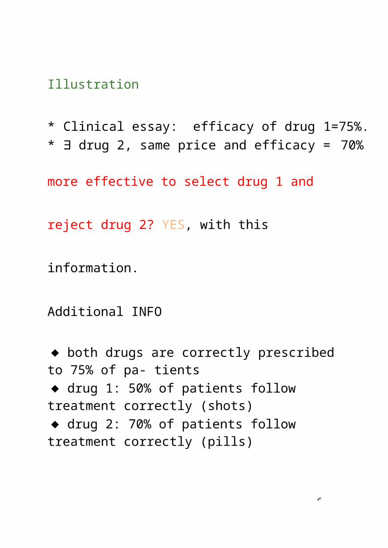
9-

- on production conditions (safety at workplace; patents; waste disposal; environmental pollution, ...)

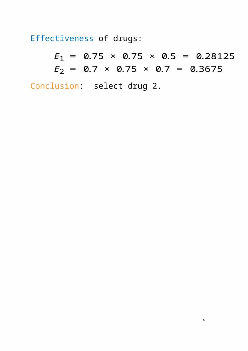
9

Reasons for regulation:

- protection of working conditions (health, safety, ...)

- protection of vulnerable social groups (kids, immi- grants, ...)

- protection of competitive conditions

- prevention of market abuse

Instruments for regulation:

- laws (antitrust agencies)

- administrative actions

- professional associations (entry conditions

Objetive of the regulation: correct market failures.

9-

Why does the State regulates the health care market?

Typology of answers:

(a) the market is too complex for patients. Providers would take advantage on them;(b) health is too a fundamental good for govern- ments let the market operate freely;(c) health care market generates externalities ( [-] epidemies, [+] vaccinations);(d) poor people must have access to the health care market;(e) asymmetric information between physician and patient (moral hazard, adverse selection).

BUT ... there are other markets for which these arguments also apply and there is no intervention (food, housing) neither in production nor in distribution.

ALSO,

- Health care market is not competitive → monopoly power, public goods, externalities, ... (see below)

9-

- Hospitals entry barriers (permissions, subsidies, ...) size (scale and scope economies) asymmetric info hospital/patient (quality,...) ownership (public, private, for profit, nonprofit)

-Physicians entry barriersprofessional associationsprivate sector: price discrimination to patients and insurers

9

Reading:

Philipson T., and E. Sun, 2008, Regulating the safety and efficacy of prescription drugs, VoxEU.orp,

[http://www.voxeu.org/index.php?q=node/804]

1

→

→

SOURCES OF MARKET FAILURE

I. Supply side

(i) natural monopolies (scale economies) large initial investment: supply of water, gas, electricity, transport, telecommunications, ...

Regulation (limit monopoly power) widely accepted (prices)

(ii) oligopolies (monopoly power) [see below]

Regulation (limit monopoly power): antitrust laws

(iii) Externalities difficult to measure, diversity of effects, diversity of types. [see below]

Regulation (limit monopoly power): OK but how?

(iv) public goods: no exclusion, no rivalry (public gardens, roads, army) [see Ch. 5]

Regulation (protect “monopoly rents”)

(v) Merit goods and incomplete markets [see below]

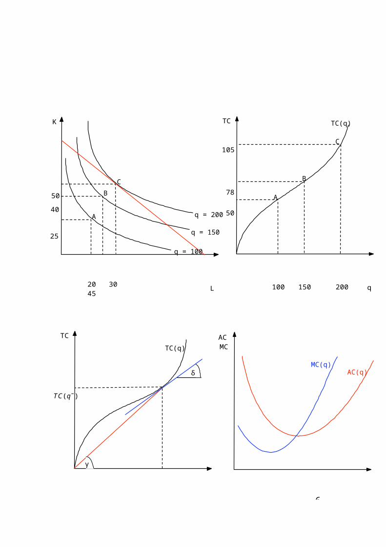
10-

II. Demand side

(i) imperfect and incomplete information on products (AIDS, drugs) and markets.

Regulation: control on sales of dangerous products; info on label of products (expiry date, ingredients,...); control on advertisement campaigns.

(ii) information as a public good → private market does not provide enough information (see below).

Regulation: increase volume of information.

1

j=1

OLIGOPOLY

Consider a market with two firms (duopoly) 1 and 2. Firm 1’s decision will be affected by firm 2’s behavior → Strategic interaction

Now, Q = ),n qj and qj/Q > 0!!

Firm 1’s decision-making process

- Market price will depend on firms production levels: P (q1, q2). Therefore, demand downward slop- ing.

1’s profit maximization: find production level solving

maxq1Π(q1, q2) = q1P (q1, q2) − C(q1)

Solucioń: q1 = f (q2)

Similarly, firm 2 maximizes profits producing

q2 = g(q1)

11-

q2

q1

q2 = g(q1)

qm1

q1∗ q1 = f (q2)

Market equilibrium

(q1∗, q2

∗) such that f (q2) is compatible with g(q1)

P

(MC=0)

Pm Monopoly

Pd Duopoly

Demand

q2∗ m

q2 Qm Q∗Q

Q∗ = q1∗ + q2

∗

MR

1

MONOPOLY

Profit maximization

maxq Π(q) = qP (q) − C(q) = I(q) − C(q)

Marginal Revenue: ∆ revenue when selling one additional unit

Marginal Cost: ∆ cost when producing one additional unit

Average Cost: Total Cost/production (unit

cost) Firm’s problem: maxq Π(q), =⇒ M R

= M C

PMC

P ∗

Profits AC

DemandCost

1

MR

q∗ q

12-

m

Monopoly power

Monopolist: pm > M C = pc ⇒ deadweightloss

P

Pm

MC

Pc

Demand

qm qcq

MR

Deadweightloss: Monopolist expels consumers un- able to pay P m → aggregate consumption ↓ (qc − q ) Remaining consumers pay higher price. Con- sumer surplus ↓ upper yellow triangle.

Monopolist sells qm at higher price, but does not produce (qc−qm) that could sell at a price > M C → Producer surplus ↓ lower yellow triangle.Note: no price discrimination

Overall loss of efficiency: yellow triangle.

12-

Health care market contains elements potentially allowing for market power:

- Hospitals with few competitors[rural vs. urban areas; specialities]

- Private hospitals w/ mkt. power[ad campaigns, contracts w/ insurers]

- Patented pharmaceutical products

- Social Security (State monoposonist pharma mkt.)

- Licences (exams) to enter the market

- Professional associations fixing minimum fees

i.e.

* Entry barriers induced or introduced by the gov- ernments to guarantee minimum quality standards, promote R&D, ...

* Government may decide to regulate non-profitable situations: transfers donations to build a hospital in a small community; offer nonprofitable services (trauma, burnt, neonatal, intensive care units).

12

B

CRITICISM: regulation may worsen situation if not adequate. BUT may improve situation if regulation is efficient.

Example: control on monopoly prices

P

APm

F

PrC

Pc

E

MC

Demand

qm qrqc q

MR

Monopolist hospital: (P m, qm) → welfare (deadweight) loss = ABC.

Government regulation: price cap P r → qr → welfare (deadweight) loss = F EC < ABC.

Problem: hospital is multiproduct service provider+ demand and technology evolve → difficult to regulate properly.

12-

Pi

),k

n

Measuring monopoly power

♠ Firm level

Lerner index: Li = Pi−M Ci ∈ [0, 1)[i’s capacity to quote Pi above M Ci]

♠ Aggregate level: 3 measures[rank firms from largest to smallest market share]

Lk =i=1 Li k

[arithmetic mean of k largest firms]n

La =

i

=1

miLi

, mi =

qi),i=1

qi

[arithmetic mean weighted by firms’ market shares]n

Lg =TT

(L − I)mi, Li /= 0

12-

i=1[geometric mean weighted by firms’ market shares]

12-

− ⇒

− ⇒

Example:

Rewrite Lerner index as (see below)

L = Pi − M

Cii Pi

m= −

ε

(i) Let εi

= 100 (very elastic)

Pi = 1.01M Ci

Li = 0.01Note 1: Pi ≈ M Ci →∼ compet behavior

(ii) Let εi

= 10/9 (very low elast)

Pi = 10M Ci

Li = 9/10 = 0.9Note 2: Pi ≫ M Ci →∼ monop behaviorNote 3: Recall P m always on elastic part of demand function

i

12

Example (cont): Let ε = −2; n = 5

m10.4

m20.25

m30.2

m40.1

m50.05

L10 . 4 − −2 =

0.2

L20 . 25 − −2 = 0.125

L30 . 2 − −2 =

0.1

L40 . 1 − −2 =

0.05

L50 . 05 − −2 = 0.025

Lk=3 =

13

3 i

=1

Li = 0.142

La = 5

i

=1 5

miLi = 0.1375

12

Lg =TT

(Li)mi = 3.323

i=1i=1

12-

tinez-Gir Mar

Xavier

Qc

Economics

Healthof

inciples Pr

1

An illustration of market power:

Welfare effects of a switch from Rx to OT C

Reading:

Tina Shih,Y-C., M. Prasad, and B.R. Luce, 2002, The effect on social welfare of a switch of second- generation antihistamines from prescription to over- the-counter status: A microeconomic analysis, Clin- ical Therapeutics, 24: 701-716.

13-

1 1

11

11

x 1


1.- description of the set-up

2a.- Drugs close to patent expiration

2b.- Drugs under patent protection

3.- Welfare effects of a switch from Rx to OT C. Re- sults:

- case a)1M CR1 x = M

COT C

LoW ambiguous

1εRx

1<

- case b)

11

1εOT C 1

11⇒

POT C < PRx

1M CR1<

M1

COT C

LoW ambiguous

13-

1

11εRx

11

1 <1

11εOT C

11

1⇒LoP ambiguous

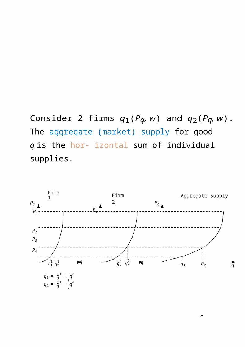
13-


July ’88 Blue Cross California request to NDAC for switching from Rx to OTC status 3 SGAs:- fexofenadine hydrochloride [Allegra - Aventis]- loratadine [Claritin - Schering]- cetirizine hydrochloride [Zyrtec - Pfizer]

Regulation: An OTC product must show safe and effective when used without supervision of a health care practitioner.

Basic economic argument of request:- cost savings due to expected price reduction in SGAs after switch- based on observed pricing for H2-receptor antagonists before and after switch to OTC statusBUTH2-receptor antagonists switch was proposed by man- ufacturers near patent expirationWHILEin SGAs case, all 3 drugs were atill under patent protection.THUS- extrapolating conclusions → erroneous- social welfare implications → uncertain.

13

B

C

demand

D

[2a] Drugs close to patent expirationArgument: after switch to OTC status, competition will lower prices → higher consumer surplus (proxy for social welfare)

P

A

P0

P1

Q0 Q1 Q

CS(P0) = AP0BCS(P1) = AP1C = AP0B + P0P1DB + DBCLo CS = P0P1DB + DBC, that is,Lo CS from ↓ price + LoCS from ↑ consumption

Strategic switch to OTC status to preempt generic competition.

13-

B

CMC

demand

D

MR

[2b] Drugs under patent protectionPatent protection grants monopoly power to manu- facturer → pricing rule: M R = M C ⇒ deadweight loss wrt perfect competitive pricing.

P

A

Pm

Pc

Qm Qc Q

CS(Pm) = APmBCS(Pc) = APcC = APmB + PmPcDB + DBCLo CS = PmPcDB + DBC, that is,Lo CS transfer to firms + LoCS deadweight loss

In addition to consider CS, discussions of welfare ef-fects of switch from Rx to OTC must consider changein deadweight loss before and after the switch.

13-

↓

AI

POT C

MCRx = MCOT C

demand demand

[3.] Welfare effects of a Rx to OTC switch 2 questions- will the price of SGAs after the switch?- social welfare consequences of the switch?

Effects on demand- Health insurance → Lo demand (moral hazard)

BUT no coverage

f→

or

consumers less price sensitive OTC drugs:

•Rx → OTC ⇒ sP → P (s: copayment rate)• demand Rx less elastic than demand OTC

P PA

PRx

MRRx

Q

Rx market (before switch)

MROT C Q

OTC market (after the switch)

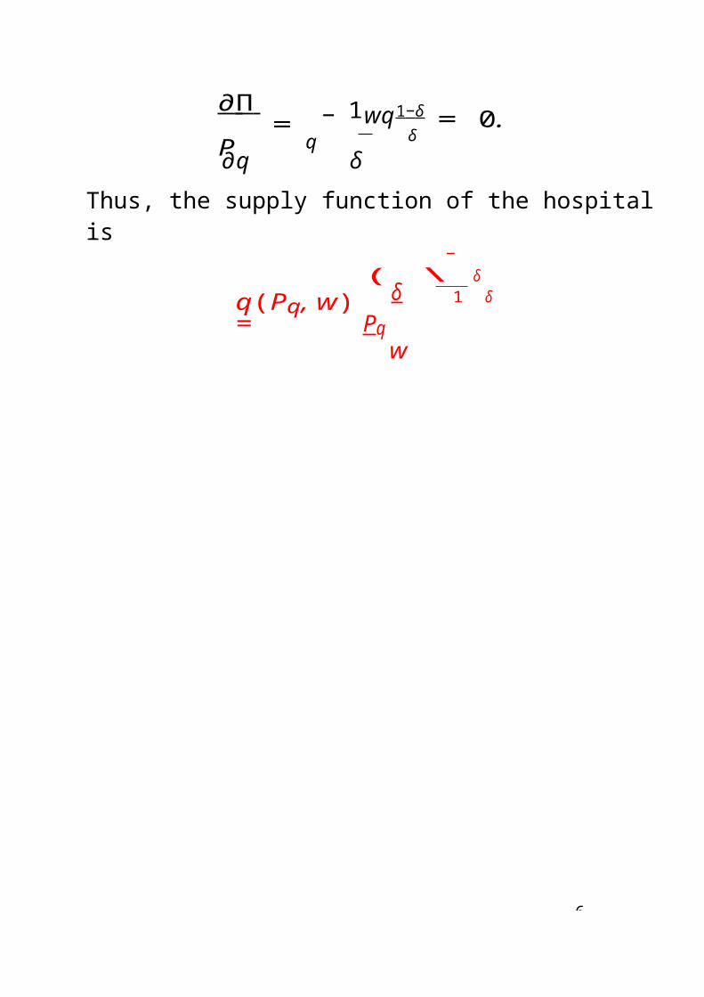
13-

Pricing strategy of a (profit max) patent holder? assumption: M CRx = M COT C

13

↓ Lo

<

- micro theory: εRx < εOT C → POT C < PRx- BUT POT C no guarantee welfare.- Consider a drug under patent

P PA

AI

PRx B

Pc

CE

POT C

BI

EI

CI

MCRx = MCOT C

MRRx

demand

Q MROT C

demand

Q

Rx market OTC market

Rx market

CS(PRx) = APRxB

CS(Pc) = APcCb.CS = PcPRxBE + BECWRx = APRxB + PcPRxBE − BEC

OTC market

CS(POT C) = AIPOT C BI

CS(Pc) = AIPcCI

b.CS = PcPOT C BIEI + BIEICI

WOT C = AIPOT C BI + PcPOT C BIEI − BIEICI

M N

DW = (M − M I) − (N − N I) > 0

M I N 1

13

signLoW depends on shape of demand curves → empirical issue

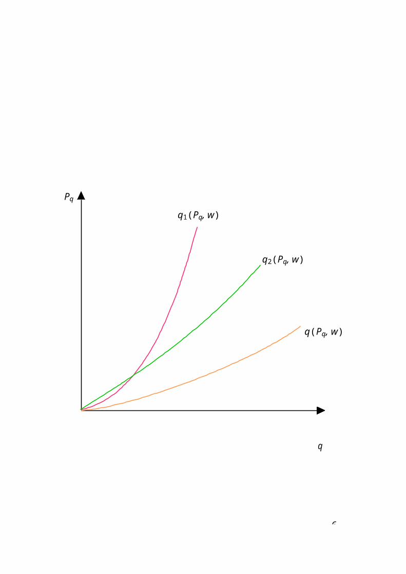
13-

AI

POT C

MCOT C > MCRx

MCRx

demand demand

Assumption M COT C > M CRx- advertising- new distribution channels- new packaging, ...

THEN

POT C may be increased after switching to OTC status

P PA

PRx

MRRx

Q

Rx market

MROT C Q

OTC market

THUS

not only welfare consequences are uncertain, but the assumption of a post switch price reduction as

13-

well.

1

Externalities

A good shows externalities when it generates third- party effects outside the price system

- positive: vaccination of my neighbors on my chances to get infected, etc.

- negative: pollution, neighbor’s loud music, etc.

Competitive market only considers private costs and benefits, not social ones → inefficiency:negative externalities → overproduction; positive externalities → underproduction.

Example: market of vaccination.

D: demand (marginal private benefit)S: supply (marginal private cost)K: marginal external benefit

Initial situation: Competitive allocation A → inefficient under positive externality K:marg. social benefit = D + K > S = marg. social cost (= marg. private cost)

14-

p

p1A

S

p2 S = S1

K

D

K

Government intervention: direct subsidy to producers of K e→ supply shifts to S

, = S − K.

New equilibrium allocation: q2 at price p2 → efficient.

q1 q2 q

1

Merit goods

Commodities that are “good” regardless of each individual’s preferences: arts, compulsory education, compulsory social insurance, ...

Individuals because of info problems are not fully aware of the benefits obtained from their consumption.

Govt. regulation: promotion of their consumption.

Incomplete markets

Private insurers may not provide coverage for some illnesses: AIDS, cancer, ...

Govt. regulation: public provision of insurance, compulsory contracts on private insurers.

1

Regulating the health care market

Definition: Regulation consists in the implementation of NON-Market mechanisms to affect the quantity, price, quality of a good exchanged in the market.

Implementation: Governmental agency (Ministry of health, ...)

Objective: guarantee a minimum level of quality, quantity, ... eliminating inefficiencies due to scale or scope economies.

Instruments:

-Monetary:

*salaries to personnel in public outlets

* reimbursement conditions to hospital (per diem, per admission, prospective, retrospective) by

1

third- party payers (public and private).

16-

2 basic mechanisms:

(i) retrospective: → ex-post

(ii) prospective: payment rates fixed prior to the period health care is provided → incentives for efficiency by limiting spurious spending. Problem: How to calculate prices?[DRGs]

-Quantity: indirect instruments. Need for approval if budget deviations → limit excess supply of facilities, promote higher use rates of existing facilities.

-Quality: Entry barriers → providers with minimum standards (physicians, nurses, pharmaceuticals); control of admission protocols, minimum/maximum in- hospital stay, adequacy of treatments, ...

16-

-Other instruments:

* licensure laws, mandates, national drug agency, universal and compulsory health insurance (public or private)

* Regulating insurance companies (∼ banks) →guarantee financial capacity

* Fiscal waives on insurance contracts

* Public health:

+ info campaigns on alcohol, tobacco, drugs, working accidents, traffic, ...

+prevention and control campaigns at schools, vaccination campaigns, ...

* Financing research in particular diseases (AIDS, cancer, ...) in public (Universities) and private (labo- ratories) research centers.

16

PPS and DRGs

DRGs instrument to determine rates of the PPS.

Def.: DRG attemps to represent a case type that identifies patients with similar conditions and pro- cesses of care.

Each DRG is given a flat payment rate calculated in part, on the basis of costs incurred for that DRG nationally.

Example

Consider a community with n hospitals and let us fo- cus in hospital 1. It faces a demand D and M C(q) = AC(q) = C0.

(a) Monopoly: provide q0 units of care at a price p0(point M ).

(b) If hospital ∈ NHS subject to retrospective reimbursement: produce at point R, i.e. AC = p → Π = 0.

16-

M

R

AC0

AC = C∗ + AFC

C∗C1

D

q0 MR q1 q

Lump-sum transfer

Incremental profit

B

(c) If hospital ∈ NHS subject to prospective reimbursement based on DRGs.

p

p0

p∗

- Assume 1 sickness- Assume hospital’s effort to reduce cost is a fixed cost.- Rates are fixed at the average marginal cost of competitors (2, . . . , n) = C∗- Also fixed cost is reimbursed as lump-sum transfer.- Thus, “new” average cost AC = C∗+AF C(average fixed cost)

16-

()

()

()

Equilibrium: point B where C∗ = D, i.e. (q1, p∗) so that Π = 0 because p = AC and f ixedcost0transf er.

Assume cost reduction yields “new” marginal cost= C∗ → hospital zero (incremental) profits.

Assume cost reduction yields “new” marginal cost= C1 < C∗ → hospital (incremental) profits =q1(C∗ − C1).

Assume cost reduction yields “new” marginal cost= C ∈ (C∗, C0) → hospital loses.

Conclusion: As hospital’s costs do not enter into the price it receives, hospital big incentive to lower cost.

1

5. Public goods

* Public goods vs Public provision of (private) goods.

↓ ↓

no rivalry because of natural monopoly

no exclusivity subsidize particular users

Examples:

PG: free highways, gardens, bridges, roads, national army, ...

PPG: private highways (tolls), mail, garbage collection, public transport, ... [exclusion if no pay]

17-

* Why does market fail?

Private market underprovides public goods → “free riders” [→ no exclusion → no incentives to finance (individual impact negligible)]

Examples:

- lack of prevention at work because of accident insurance

- “free ride” in the bus

- inhabitants of BCN using public gardens in Sant Cugat

- avoid vaccination when everybody gets vaccinated (The Economist 11-4-98)

Conclusion: underprovision by private markets →government regulation.

17-

Are health care services public goods? NO!

- there is rivalry (services to a patient cannot be si- multaneously provided to another)

- there may be exclusion (if patient cannot pay, may be excluded)

⇒ Health care services: private good publicly provided

BUT

INFORMATION is an economic good with a high component of public good:

- getting info by one individual does not limit possibilities to ohers.

- although information has a price, the cost of providing information to an additional individual is negligible (advertising campaigns, mailings, ...)

⇒ private market underprovides information → public provision. How to do it?

17

- help disseminating info (public provision or transfers to private provision)

- increase information participating in scientific research (public provision or transfers to private provision)

ALSO

Donations (charity) have characteristic of a public good: help people with low income levels to improve consumption (also health care)

Individual donations are small in the aggregate → free riding [donation to help victims of natural disas- ters ...]

How to implement these donations? (i) additional income free to use; (ii) transfer with a predefined use → problems of equity, efficiency, need, ...

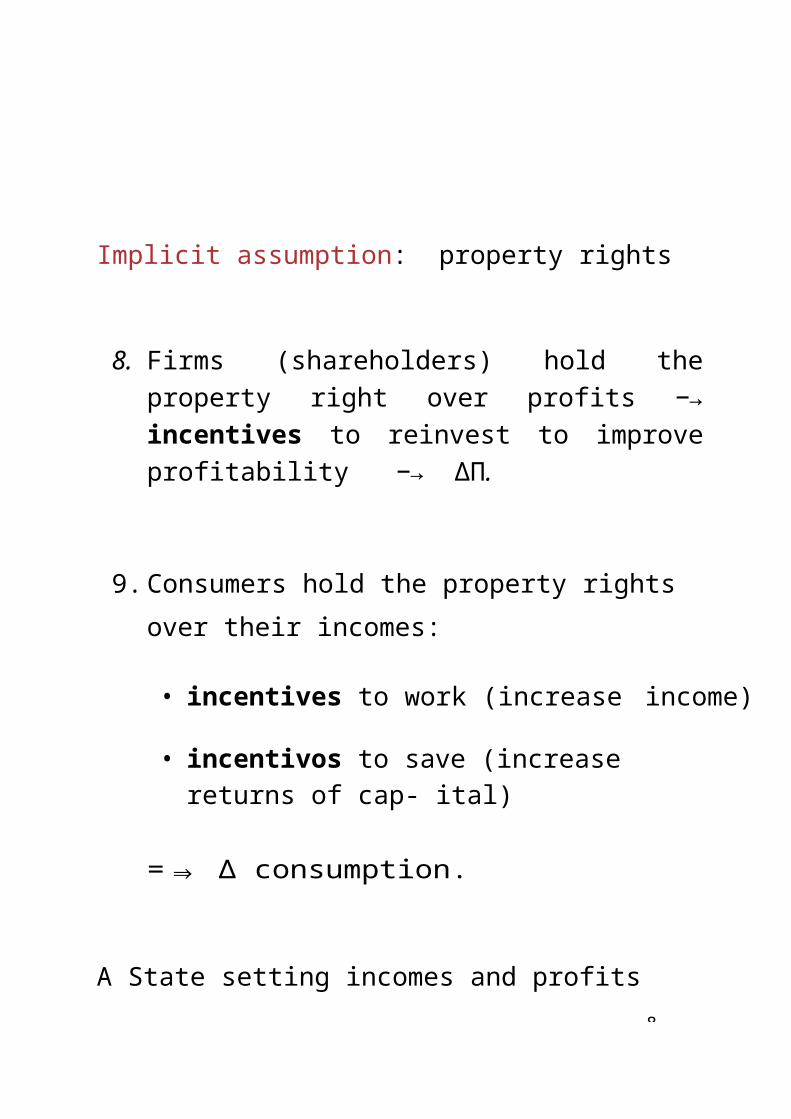
17-

Reading

Clinical trials as a public good:

Lewis, T.R., J.H. Reichman, and A.D. So, 2007, The case for public funding and public oversight of clinical trials, Economists’ Voice, 4: article 3.

http://www.bepress.com/ev/vol4/iss1/art3/

1

6. Nonprofit Enterprises/Organizations (NPE)

NPEs are important in the health care market (hospitals and nursing homes):

Definition: A NPE is an organization where nobody holds property rights on profits =⇒

- allows for objectives /= max. profits,

- exempt from corporate taxes (profits, VAT, ...)

- donations to NPEs receive special fiscal treatment

18-

Why do NPE exist?

2 reasons: (i) market inefficiencies, (ii) asymmetric information

(i) Market inefficiencies (not solved by governmental regulation)

3 types of firms in a market:

- for profit private firms,

- public firms,

- Nonprofit firms (public and private).

Public firms appear to correct market failures (externalities, public goods) but no guarantee of efficiency.

* Externalities → private market yields underprovision → inefficiency. Why?

18-

Example 1: vaccination for influenza.

- Individual ↓ fall sick (private benefit)

- Individual ↓ infect others (social benefit): External- ity.

Free markets: individual only computes private benefits → ignore social benefits → market delivers quantity lower than max social benefit → inefficiency.

Government reaction: public firm to provide a public good → avoid free rider problem.

BUT does not guarantee efficiency (potential inefficiencies of governmental activities may offset potential gains)

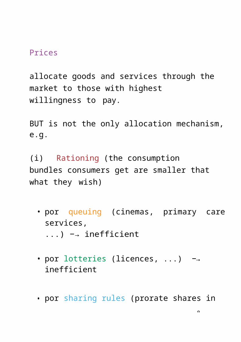
18

Health of

nciples

Example 2: campaigning for provision of a public good.

Society with 5 individuals: common marginal income tax (MIT).

Government proposes building a hospital for children. Question: how big (how many beds)? VOT- ING (majority rule)

Individual demands Di, (i = 1, 2, 3, 4, 5)

Voting outcome for the different alternatives:

18-

M

artinez-

Xavier

Government provides C beds, every individual will pay c × M IT and fiscal revenues = cost of the project. (Individuals 4,5 vote for C as a “second best” alternative).

Conclusion: Voting only satisfies individual 3 for whomM IT = marginal benefit.

Consequence: government inefficient in providing the public good → individuals 4,5 form a NPE and provide the rest of the public good.

18-

Application to the health care sector.

Health care is a private good (exclusion, rivalry) with externalities.

Hospitals and nursing homes → room for NPE when there is enough dissatisfaction with public provision

↓

- non-governmental organizations (greenpeace, medicus mundi, xxx sans frontie` res, ...)

- origin of hospitals as charitable institutions re- lying on donations.

18

(ii) Asymmetric information

Different argument: difficulty in writing a complete contract because quantity or quality are not (perfectly) observable by the purchaser.

Example: assistance 3rd world.

Too costly to verify that a for-profit firm delivers goods to targeted population → delegate in a NPE.

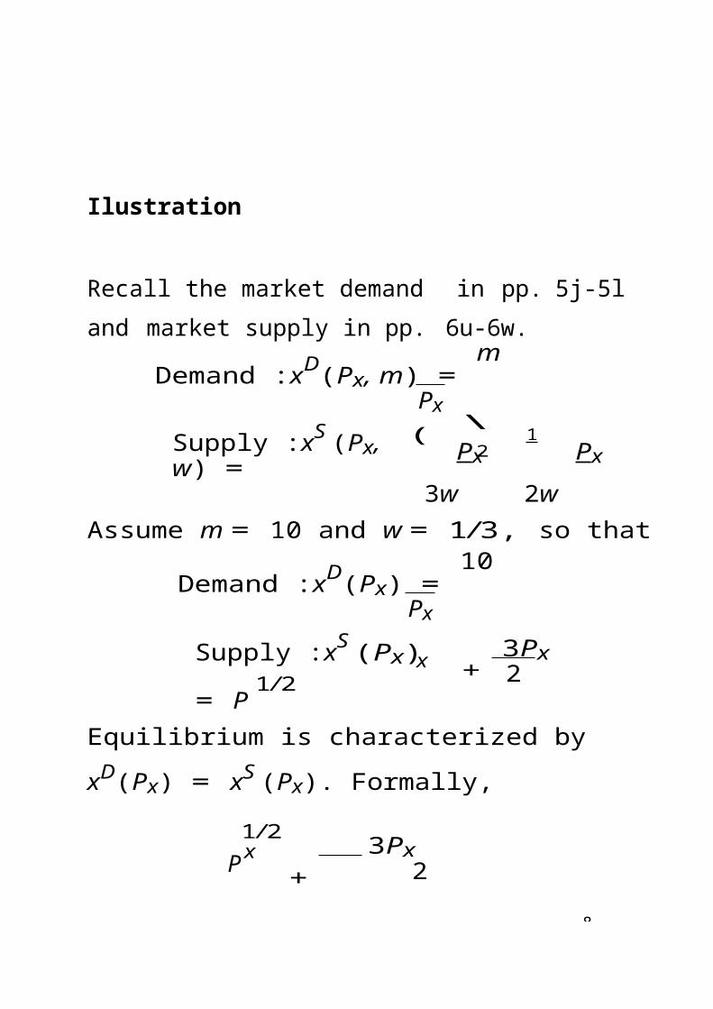
18-

Example: nursing home

Similar to hotel management (rooms, housekeep- ing, meals, recreation facilities)

Differences

hotel max profit s.t. satisfaction of clients

nursing home clients (patients) are not able to evaluate quality of the service given their health state. Relatives only partial info.

* If nursing home is for-profit, may arise conflict of interest with some clients.

* Empirical evidence: quality of services nonprofit nursing homes not inferior to for-profit nursing homes.

Comment Not easy to reach consensus on quality criteria → proxies: observable signals (variation in health state of inmates, ...)

1

H Final health state

What is a hospital

1.- What does a hospital do?

Patient

Initial health state (treatment) discharge/

death

Emergency

2.- Hospital’s idiosyncrasy

• personalized treatment to every patient• detailing → distort treatment selection• moonlighting → distort allocation effort/quality• resource hoarding

PCC/OPV

( )

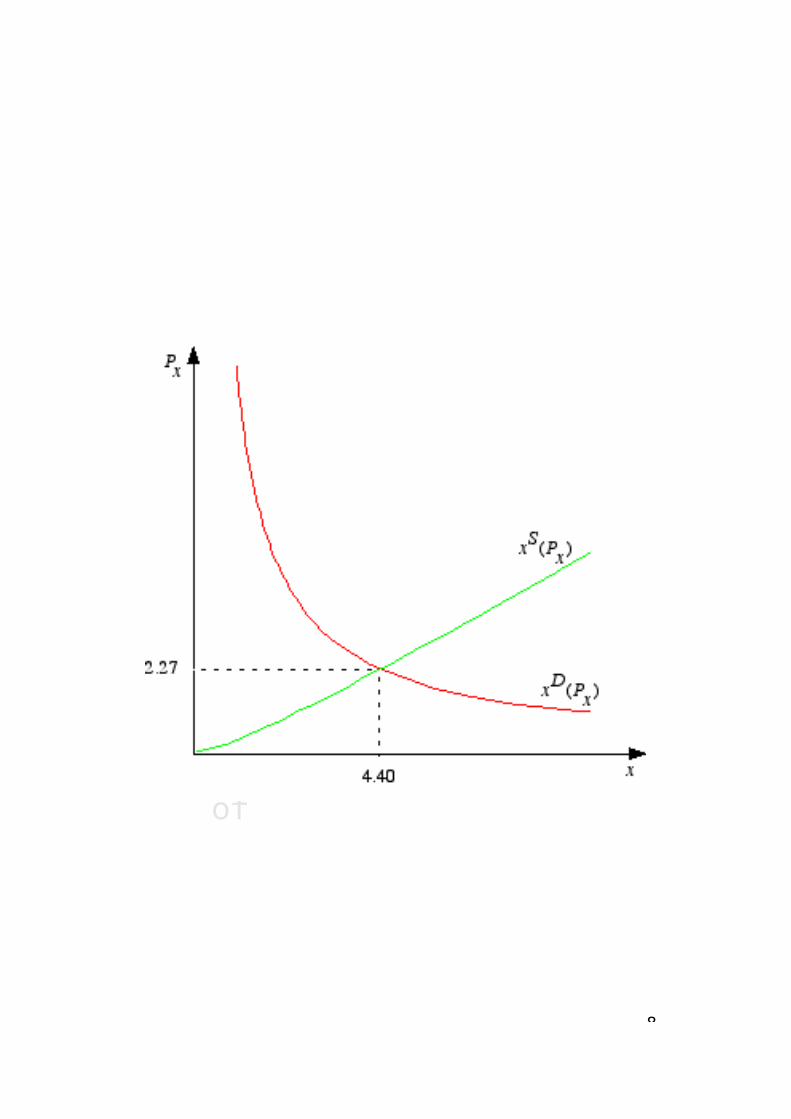
19-

3.- Measures of activity

♠ # patients treated:

- aggregate

- per DRGs

- per discharges/out-patient visits/emergency room episodes

♠ mortality rate

- Summary

Hospital unit of multiproduct services →

❑ Scale economies

❑ Scope economies

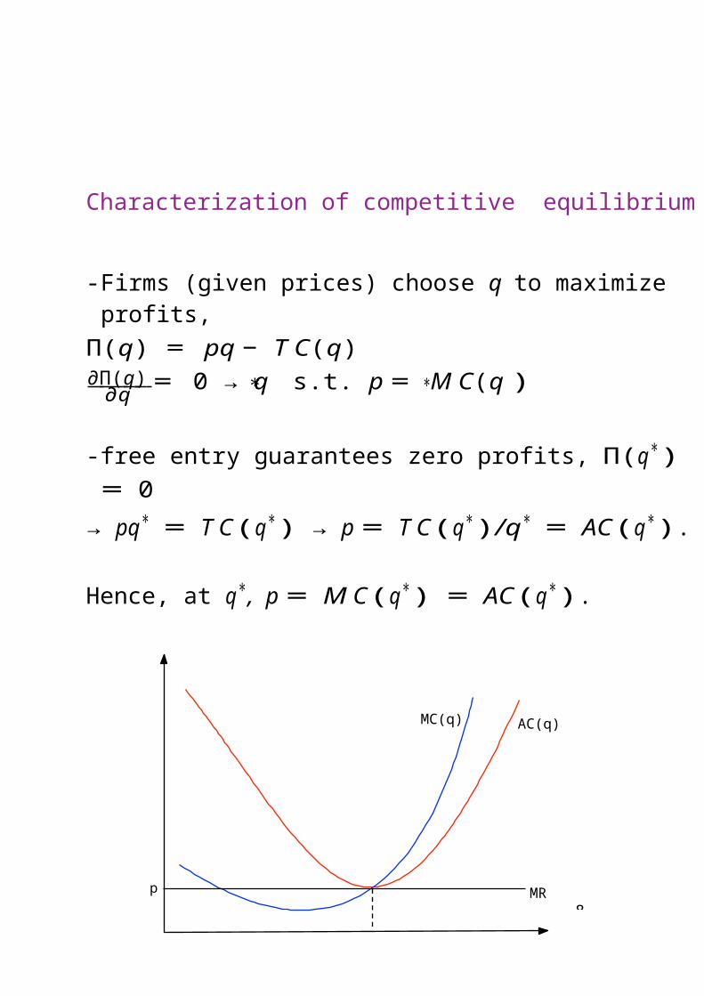
2

Modeling a hospital as a NPE

Three initial lines of research:

(a) Quantity vs. quality: Newhouse (1970)

max U (Q, q) s.t. Π = 0Q,q

(Q, q): (Quantity, quality) of health care services.

(b) As a cooperative Pauly-Redisch (1973)

maxM

net hosp. revenues#physicians in

coop.HR ∼ Π. Closed/open

cooperative. (a), (b) comparable

(c) NPE vs. FPE Harris (1976)

Efficiency NPE vs. efficiency FPE, via property rights

basic argument:manager reimbursement: trade-off between pecuniary & non- pecuniary components

2

NPE: ↓ salary, ↑ NPI than FPE

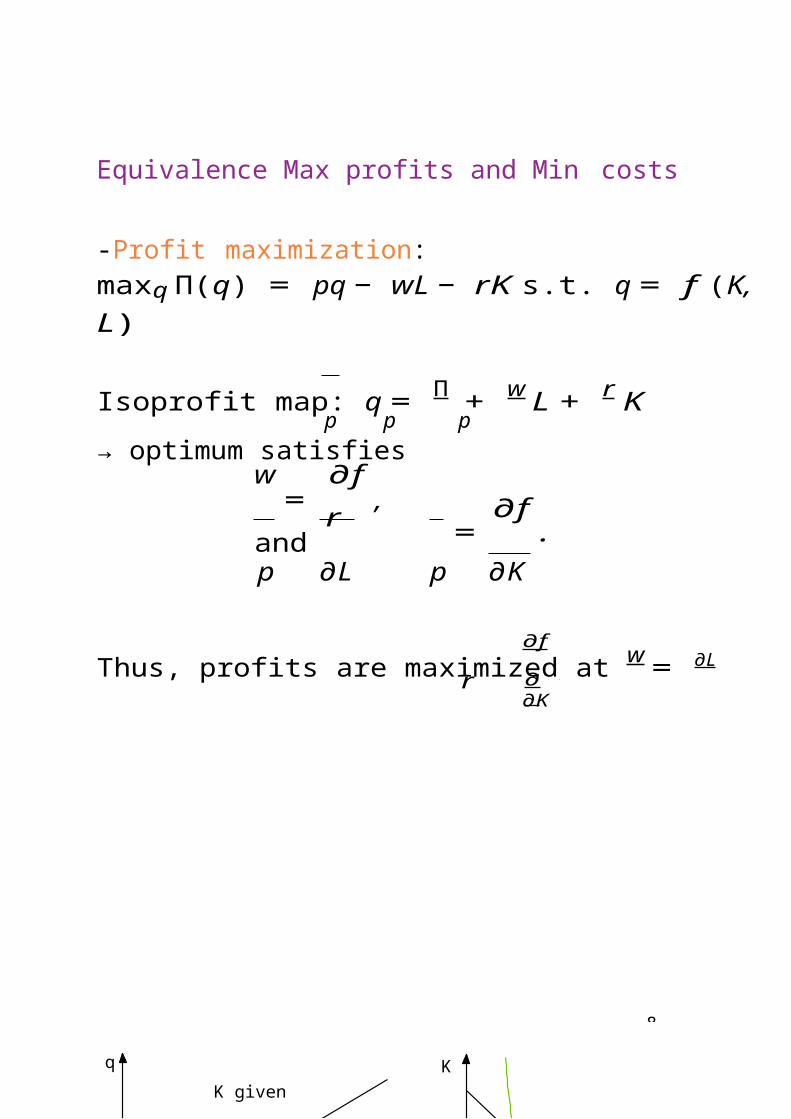
20-

→

Modeling a Nonprofit hospital (I): Newhouse (1970)

Organization of a hospital as a NPE: 3 decision- making parties:

- Board of trustees → patrons /= profiles,

- Hospital administrator (CEO) → agent of trustees,

- Physician staff.

Assumption 1: complex decision-making single utility function.

Assumption 2: Utility function U (Q, q) defined over single sickness.

Q quantity of output (cases treated/time period);

q quality of output: index aggregating physician staff expertise, hospital facilities, nursing care to patients, ...

Objective of the hospital: select (Q, q) to max U (Q, q) given budget constraint (revenue form donations and patients = cost).

20-

M

Xavier

Qc

of

Demand of health services depend on quality D(qi).

Costs of hospital depend on quality. Average costAC(qi)

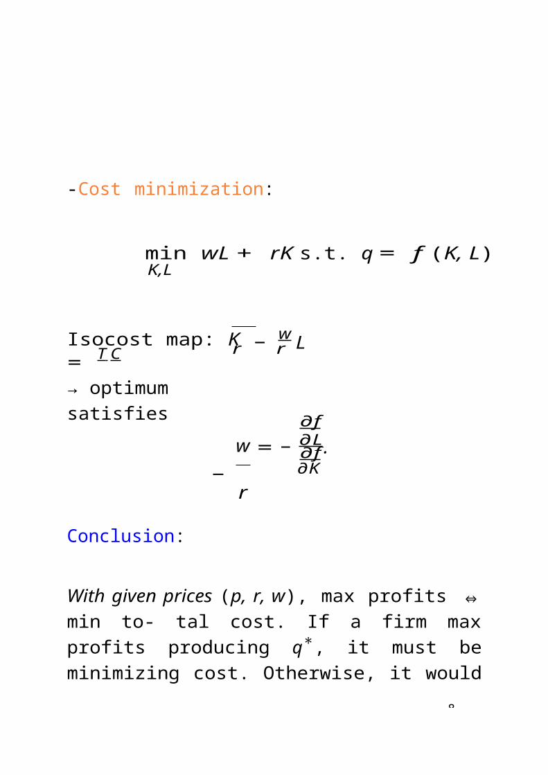
20

Xavier

Qc

Economic

s ealth

Approach 1 (Equilibrium): given a quality level q1, budget constraint (i.e. zero-profit condition) requires demand = average cost ⇒ Q1

Note: D = AC ⇒ Π = 0

P (Q) =

C(Q)

Q⇔ P (Q)Q = C(Q) ⇔ Q(Q)Q−C(Q) = 0 = Π

20-

Economic

s Healthof

ciples

ALERT: Quality and quantity non-monotonic rela- tions:

If patients evaluate an Lo in quality q1 → q2 more than an Lo increase in cost, we obtain Q1 < Q2, i.e. Loq → LoQ.

If average cost of providing a high level of quality q3 is higher than consumers willingness to pay D(q3), we obtain Q3 < Q2, i.e. Loq → yQ.

20-

Mar

Xavier

Qc

Economics

Approach 2 (Equilibrium): find (Q, q) that max U (Q, q)given budget constraint, i.e. Π = 0.

Equivalently, find Q − q frontier (feasible set) and combine with utility levels (indifference map).

Hospital problem:

max U (Q, q) t.q. (Q, q) ∈ frontier Q − q

2

M

MM

Modeling a Nonprofit hospital (II): Pauly-Redisch (1973)

Hospital as a physicians’ cooperative to maximize their net income.

Assume revenues only from bills to patients (no donations) → price of care determined by demand.

Supply of health care services depends on quantity of inputs: capital K, (non-technical) labor L, and physicians M .

Objective of the hospital: max net revenue per physician max HR, where

HR = revenues − payments to (K, L, M ).

Let M ∗ denote the optima number of physicians closed staff cooperative.

Given (K, L)

HR ↑ if M < M ∗, and HR ↓ if M > M ∗.

21-

M

artine

Xavier

If open staff cooperative and competitive physicians market →

physicians supply perfectly elastic S → optimal number of physicians Ms.

In any case, contracting of (K, L) according to M ∗

or Ms.

2

Newhouse vs Pauly-Redisch

Simplifying assumptions

* Combine hospital and physicians revenues in a single function R(Q, q)

* (Q, q) depend of (K, L, M )

* Other hospital revenues: donations D + transfers (subsidies) G

* Perfectly competitive physicians market: price s

* Perfectly competitive capital market: price r

* Perfectly competitive labor market: price w

Hence,

HR = R(Q, q) + D + G − (wL + rK + sM )

22-

Mar

Xavier

Qc

Economics

Health

Pauly-Redisch: max HR → HR appropriated by cooperative.

Newhouse: max U (Q, q) s.t. HR = 0 Solution: A

Different outcome because cooperative when ap- propriating HR includes D and G. It is “as if” hospital would be a cover for a for-profit organization →

Policy conclusion: eliminate G and corporate tax ex- emptions.

22-

Economic

s Healthof

iples

Comment: Is it possible Pauly-Redisch → Newhouse?

YES, under some conditions, e.g.

Lo competition among hospitals (free entry). If demand ∼ constant, HR ↓. Limit case HR → 0.

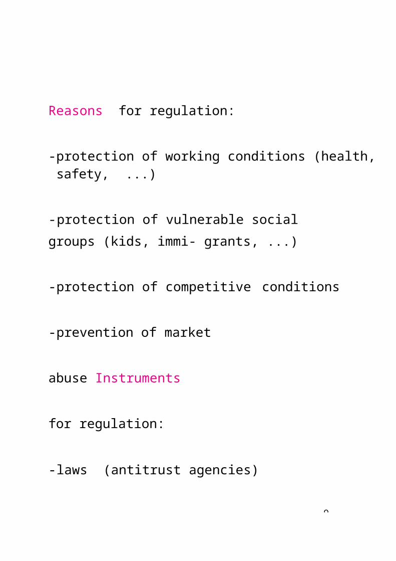
2

Modeling a Nonprofit hospital (III): Harris (1976)

Aim: compare efficiency NPE vs FPE → theory of property rights

The theory of property rights

Private firm: owner holds property rights on net profits → may sell those rights (shares, ...)

Large private firms: property /= management. Man- agers are agents of owners BUT imperfect agents because,

* Cost of monitoring the manager → owner accepts deviations from max Π.

* in particular, manager also obtains “non pecuniary income” (NPI) → manager’s utility depends of Π and NPI .../...

23-

Xavier

Qc

Economics

Health

.../... in turn, NPI will affect wealth generated by firm (profits). Hence, trade-off (Π, NPI)

Example Hospital management opens a heart surgery outlet, not profitable but prestige → economic result (profits) will be affected.

23-

Economic

s Healthf

es

Property rights and for-profit enterprises

FPE: selects feasible (Π, N P I) to max U (Π,

N P I). Solution: A

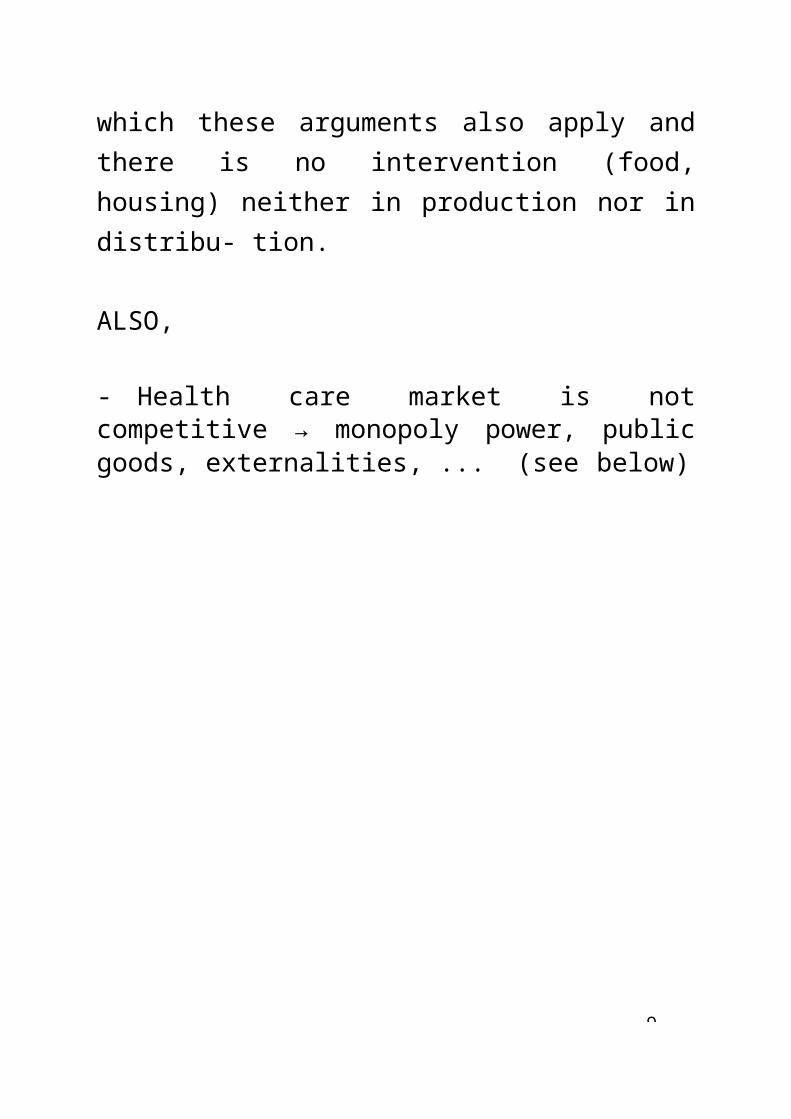
23

Economic

s Healthof

es

Property rights and nonprofit enterprises

NPE’s problem: set manager’s wage to avoid appro- priation of profits → 2 restrictions:

- feasible (Π, N P I) [1]

- max salary: L [2]

NPE: selects (Π, N P I) to max U (Π, N P I) s.t. [1] and [2]

Solution: lower salary and higher NPI.

If NPI involve excessive non productive activities, NPEs less efficient than FPEs.

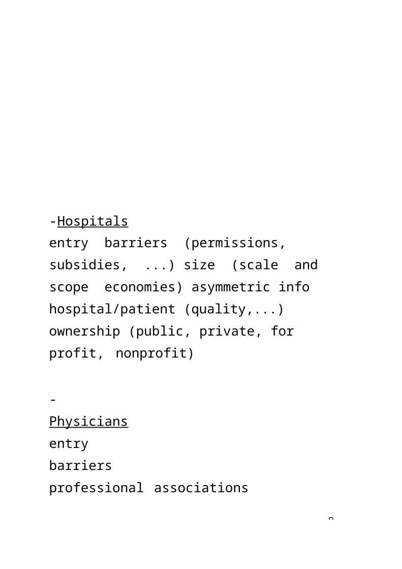
23-

Conclusion

- (III) is a different model because hospital does not max profits as managers are imperfect agents.

- NPE no access to incentives on profits but in models (I) and (II)hospitals take efficient decisions.

- more adequate model? → empirical evidence:

* no significant differences between nonprofit and for-profit hospitals ⇒ models (I) and (II) better than (III).

* significant differences between nonprofit and for-profit nursing homes ⇒ model (III) better than(I) or (II).

23-

Lines of development of literature

♣ 1 illness → several illnesses

♣ random demands (epidemic events, accidents,...)

♣ emergency vs. regular health care services

♣ primary health care integrated/segregated hospital care

♣ estimation of hospitals’ PPF: technical efficiency,...

♣ etc.

23

Reading

Eggleston, K., Y-C. Shen, J. Lau, C.H.Schmid, andJ. Chan, 2008, Hospital ownership and quality of care: what explains the different results in the literature, Health Economics, 17: 1345-1362.

http://www3.interscience.wiley.com/journal/121519547/issue

2

7. Preventive vs. Curative Medicine. A health policy exercise

The general set-up. Identify tools to incentivate:

- Patients to develop healthy habits- Insurance companies, to provide preventive medicine coverage.

Initial scenario:

- Insurer covers hospital and treatment expenses.- Patient losses salary and bears pain.

⇒ split responsibility between insurer and insuree.

⇓

Insurance contracts do not cover both demand sources→ underinvestment in preventive medicine.

⇓

Socially, investment in preventive medicine is profitable. BUT insufficient individual incentives.

24-

Example [Helwege, 1996]

Thesis: Policy misdesign because ignores some in- teractions among agents (patients, insurer)

Compute costs of preventive vs. curative measures in men with high risk of heart attack.

Preventive measures:- Weight control- Yearly check-ups and cholesterol control.

Curative measure:- Hospitalization and treatment of heart attack.

24-

Data:1. Population: Men, 50 years old (today).*15% will suffer a heart attack before age 65;* average age of heart attack: 60.

2. Cost of treatment : 30,000 e/individual

3. Cost of weight control : 50 e/individual/year

4. Cost of check-up: 200 e/individual/year

5. Incidence of weight control on risk: 5%

6. Incidence of weight control on cost: (0.05)(30,000)=1,500 e/year (for 10 years).

7. Incidence of check-up on risk: 20%

8. Incidence of check-up on cost: (0.2)(30,000)= 6,000 e/year (for 10 years).

9. Interest rate: 5%

24-

10. Individual’s loss due to heart attack: 100.000 e

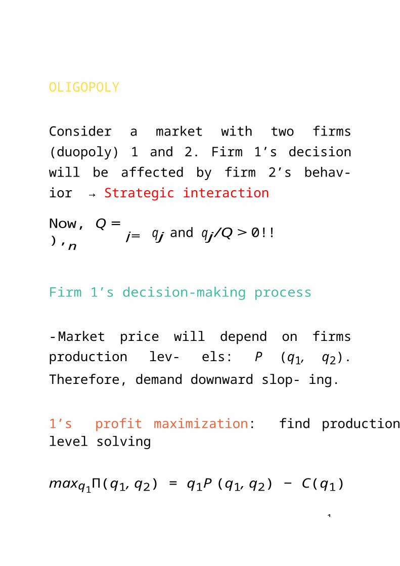
24

Discounted present value (time value of money)

[money today is more valuable than money in the future by the amount of interest that money can earn.]

Compute the investment today at a return rate of 5%, so that in three years we will receive 100 EUR:

x(1.05)3 = 100100

x = 1.053 = 86.383759

In general, the present value of a capital K to be available in n years at the interest rate r is given by,

K

Example:

x = (1 + r)n

- 1EUR at r = 5% in 10 years: 1.0510 = 1.629

- present value in 10 years of weight control:

501.629 = 30.69

- present value in 10 years of check-up:

200 1.629

24

= 122.77

24-

Discounted present value: two approaches

(i) Value of 100 e today in 3 years discounted at 5%

t = 0 : 100t = 1 : 100 + 5%(100) = 100 + 5 = 105t = 2 : 105 + 5%(105) = 105 + 5.25 = 110.25t = 3 : 110.25 + 5%(110.25) = 110.25 + 5.5125 =

115.7625

Summarizing: y = 100(1.05)3 = 115.7625 e

(ii) Capital to invest to day at 5% interest rate so that in three years it is 100 e

x(1.05)3 = 100100

x = (1.05)3 = 86.38

That is investing today 86.38 eat 5%, yields 100 ein three years.

24-

Costs of performing weight controls and check-ups along 15 years

Year Discount Weight control Check-up0 0 50 200

190.48181.32172.71164.47156.74149.25142.15135.41128.95122.77116.96111.36106.04101.01

200 1.05

200 (1.05)2

200 (1.05)3

200 (1.05)4

200 (1.05)5

200 (1.05)6

200 (1.05)7

200 (1.05)8

200 (1.05)9

200 (1.05)10

200 (1.05)11

200 (1.05)12

200 (1.05)13

200 (1.05)14

1 1.050 47.622 1.103 45.633 1.158 43.184 1.216 41.125 1.276 39.186 1.340 37.317 1.407 35.548 1.477 33.859 1.551 32.2410 1.629 30.6911 1.710 29.2412 1.796 27.8413 1.886 26.5114 1.980 25.25

Total 544.90 2179.62

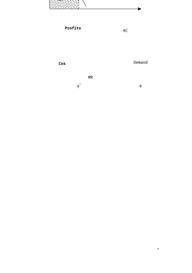
24

Insurer’s incentives to invest in prevention in one individual

* Expected cost of a heart attack (to happen in 10 years):

(0.15)(30000) = 4500 eDiscounted present value of this expected cost:

45001.0510 =

45001.629

= 2762.43 e

* Expected cost savings from weight control (5%):

(0.05)(2762.43) = 138.12 e* Expected cost savings from check-ups (20%):

(0.2)(2762.43) = 552.48 e* Discounted present value of cost weight control along 15 years: 544.90 e* Discounted present value of cost check-ups along 15 years: 2179.62 e

Conclusion

138.12 < 544.90552.48 < 2179.62

Insurer does not provide contracts with coverage for

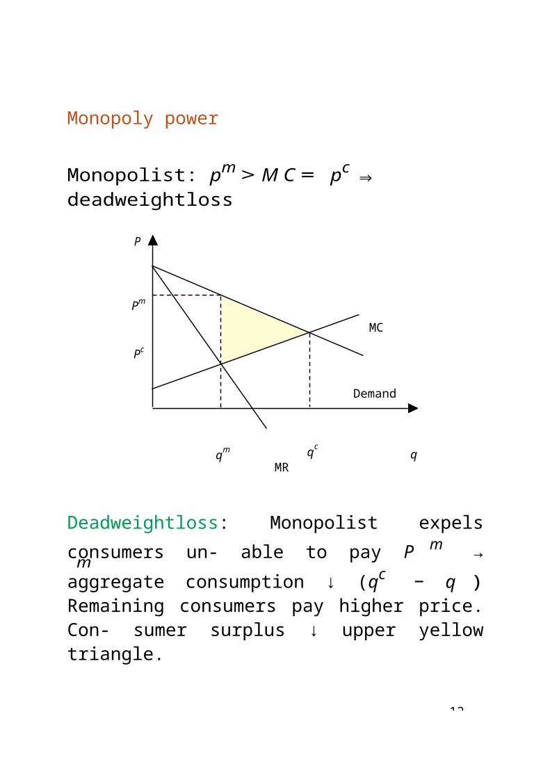
24

preventive services. [neither separately nor together]

24-

Patient’s incentives to invest in prevention

Patient’s loss: 100000 e(wage, pain, ...)* Expected loss from a heart attack (to happen in 10 years time):

(0.15)(100000) = 15000 eDiscounted present value of this expected loss:

(15000)1.0510 =

150001.629

= 9208.10 e

* Expected cost savings from weight control (5%):

(0.05)(9208.10) = 460.40 e* Expected cost saving from check-ups (20%):

(0.2)(9208.10) = 1841.62 e* Discounted present value of cost weight control along 15 years: 544.90 e* Discounted present value of cost check-ups along 15 years: 2179.62 e

Conclusion

460.40 < 544.901841.62 < 2179.62

Patient does not invest in preventive medicine (healthy

24-

habits). [neither separately nor together]

24-

Joint patient-insurer incentives to invest in prevention

* Expected cost savings from weight control:

138.12 + 460.40 = 598.52 e* Expected cost savings from check-ups:

552.48 + 1841.62 = 2394.10 e* Discounted present value of cost weight control along 15 years: 544.90 e* Discounted present value of cost check-ups along 15 years: 2179.62 e

Conclusion

598.52 > 544.902394.10 > 2179.62

The alignment of incentives of insurer AND patient makes investment in prevention profitable.

2

/

Comments

(i) Technological change increases uncertainty in computation of costs. Compare

y treatment costsy preventive costs

> 1 ⇒ prevention less attractive

(ii) Valuation of risk and benefits of prevention.* Common objection: psychological costs> hospital costs+ loss of income. Maybe, but not for everybody.

* Willingness to pay vs. willingness to accept compensation. Common problem in cost-benefit analysis.

Example 1. Money parents willing to pay to prevent death of an offspring = money they would accept as compensation after death of that offspring.

Example 2. Patients that cannot afford paying for drugs to prevent cholesterol, need not be willing to accept compensation of 30000 e to

2

have a heart attack.

25-

(iii) Patients’ information Imperfect info on:* expected loss from a health crisis;* risk of suffering a health crisis;* benefits of prevention.

⇒ info campaigns to induce healthy habits.

(iv) Patients’ risk aversion.

(v) Preventive free services:* physical exercise;* use of seat belts in cars.� Why not? Difficult answer: psychology.

2

How to solve inefficiency?

(i) Agreements insurer/insured: y premiums if insured also contracts preventive services.

• insurer must invest in monitoring• compare (monitoring cost + y revenues) withhospital cost savings.

BUT

* variety of illnesses and risk attitudes → largemenu of discounts (hard to manage)

* high risk groups may not be able to control all elements of risk.

* preventive treatments (with medicines) may have side effects (trigger other illnesses).

* low income patients may not have access to discounts in premiums.

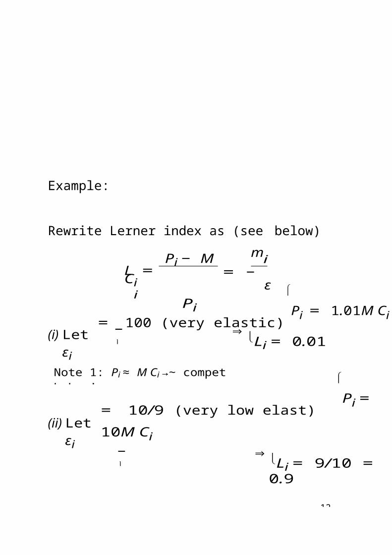
26-

(ii) Government subsidies to insurer and insuree to incentivate prevention.

BUT

* best use of tax revenues?

* may be justified for public goods. Health Care services are not.

* tool to redistribute income. consequences:

../ who benefits from it?

../ who finance it (via taxes))?

(iii) General information campaigns.

26-

Readings

- on incentives in healthy habits:

Helwege, A., 1996, Preventative versus Curative Medicine: A Policy Exercise for the Classroom, J. of Economic Education, 27: 59-71.

- on preventive care:

Hennesy, D.A., 2008, Prevention and cure efforts both substitute and complement, Health Economics, 17: 503-511.


- on prenatal care:

Conway, K.S., and A. Kutinova, 2006, Maternal health: does prenatal care make a difference?, Health Eco- nomics, 15: 461-488.


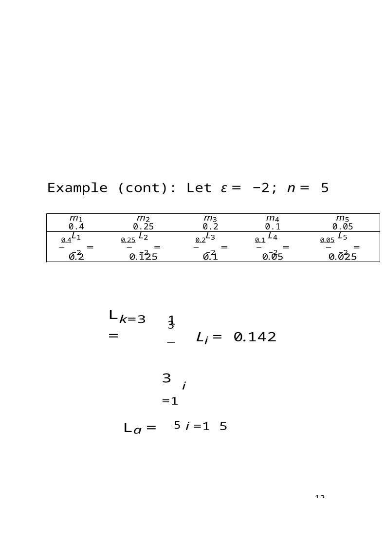
2

1

8. Uncertainty, Risk and Insurance

Individual: income Y , Utility U (Y ).

Two states: healthy, sick (prob. p) → Yh, Ys

• Expected income: ex-ante average income weighted by p: E(Y ) = pYs + (1 − p)Yh• Utility of expected income: U (E(Y ))• Expected utility : ex-ante average utility weighted by p: E(U ) = pU (Ys) + (1 − p)U (Yh)

Ilustracioń

p = 1/3Ys = 0 ⇒ E(Y ) = 1(0) + 2(150) = 100

3 3Yh = 150

1

U (Y ) = Y 2⇒ U (E(Y )) = 1002 = 10U (Ys) = U (0) = 0

U (Yh) = U (150) = 12.25

E(U ) =

1(0) +

2

3 2

(12.25

) =

8.163

27-

Crucial elements of the analysis:

(a) E(U ) vs. U (E(Y ))

(b) Uncertainty vs. risk

Individual behavior facing probability of illness?

Distinguish Uncertainty and Risk

Def.: Risk

Individual can assign probabilities to the different states he may face.

Def.: Uncertainty

Probabilities of the different situations are exogenous.

27-

Example 1 (Risk): 2 situations

1. Careless driver:

Prob 1/10,000 → accident

Prob 9999/10,000 → no accident

2. Careful driver:

Prob 1/100,000 → accident

Prob 99,999/100,000 → no accident

Remarks

1. Driving style is a choice variable.

2. Occurrence of accident no proof of careless driving.

3. Occurrence of acccident is observable.

27

Example 2 (Uncertainty): 2 situations

1. Able physician:

Prob 1/100 → wrong diagnose

Prob 99/100 → correct

diagnose

2. Lesss-able physician:

Prob 2/100 → wrong diagnose

Prob 98/100 → correct diagnose

Remarks

1. “Ability” is not choice variable.

2. Occurrence of wrong diagnose no proof of lack of ability.

3. Wrong diagnose is observable.

27-

Three attitudes towards risk. Two alternatives: participate in a risky situation → E(U ); do not participate → U (E(Y )).

Def.: Risk aversion: E(U ) < U (E(Y )).

Def.: Risk neutrality: E(U ) = U (E(Y )).

Def.: Risk preference: E(U ) > U (E(Y )).

U(Y)

U(Yh)Upr(Y) Unt(Y)

Uav(Y)

Uav[E(Y)]

E(U) Unt[E(Y)]

Upr[E(Y)] U(Ys)

YYs E(Y) Yh

27-

Example 1: tossing a coin

Individual: Y= 49 e, U (Y ) = √

Y .

Alternative 1. Participate in a lottery: toss a

coin. If win → 98 e. If loss → 0 e.

Cost of participation: 49 e.

Expected utility:1 1

E(U ) = U (49 + 98 − 49) + U (49 − 49) =2 2

1

2U (98)

+

1

2U (0) ≈ 4.9497

Alternative 2. Do not participate → U (49) = 7 (In this case, Y = E(Y ))

Conclusion: E(U ) < U (E(Y ). Risk averse individual decides not to participate.

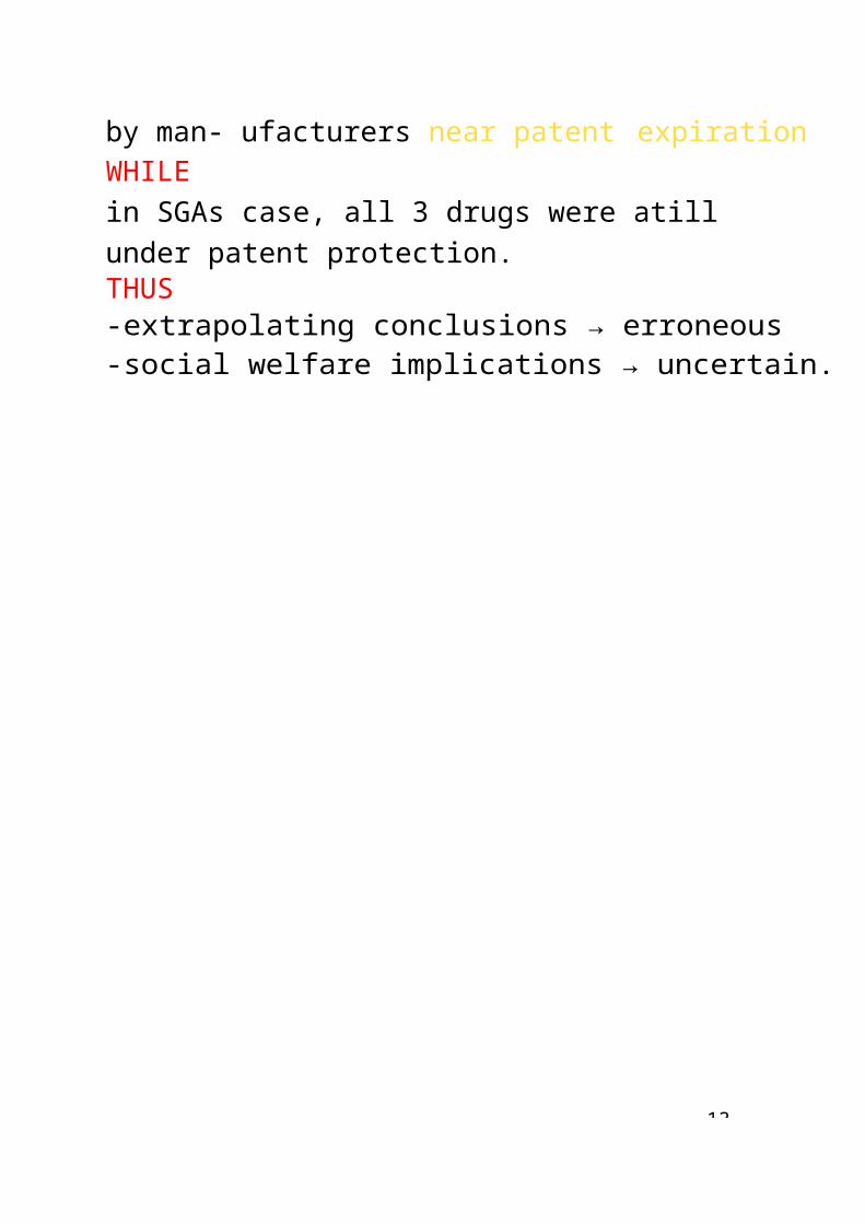
27-

Remark: U (Y ) is strictly concave.

27

−

−

How can the individual be induced to participate?

- Lo payment if winning: e.g. 256 e1

E(U ) = U (49 + 256 49) +

2

1

2U (49 − 49) =

1U (256)

+2

1U (0) =

2

116 = 8 > 7

2

-y participation cost: e.g. 24 e

1E(U ) = U (49 + 98 24) +

2

1

2U (49 − 24) =

1

2U (147)

+

1

2U (25) ≈

112.1243 +

15 ≈

2 26.0622 + 2.5 ≈ 8.56232 > 7

27

Remark: either way implies rising the expected value of the lottery. The seller of the lottery tickets would make a loss for sure if selling many tickets!

27-

99% −→ 21000 e

99% → 20940 e(= 21000 − 60)

Example 2: contracting insurance

Individual with assets valued 21000 e.

Probability of losing 6000 e= 1%

Probability distribution:1% −→ 15000 e

Insurance: alter probability distribution

Insurance contract:- indemnity = 6000 e- premium = 60 e

New probability distribution:1% → 20940 e(= 21000 − 6000 + 6000 − 60)

Equal wealth in both states of nature: Individual fully insured against loss.

2

−

• →•• →

1

1

1

1

1

Healthcare insurance

Risk aversion → contract healthcare insurance.

*Demand of insurance Recall:• Individual: income Y , Utility U (Y )

concave. Two states: healthy, sick (prob. p) Yh, Ys L loss of income if sick.Protection against loss L insurance indemnity:

Z e when sick. Premium: αZ e.

How much insurance to buy? (i.e. choose the value of Z to max E(U ))

Ys(Z) = Y − L − αZ + Z = Y − L + (1 − α)Z Yh(Z) = Y − αZFormally,

max E(U ) = pU (Ys) + (1 p)U (Yh)Z

Solution:∂E ( U ) = p

∂U 1

11

∂Ys ∂U+ (1 − p) 1 ∂Yh

∂Z ∂Y 1Ys ∂Z

1

∂Y 1Yh ∂Z

∂U= (1 − α)p 1 ∂U− α(1 − p) 1 = 0

2

∂Y 1Ys ∂Y 1Yh

28-

− α p

∂Yh

InterpretationConcave utility → decreasing marginal utility.♠ Each extra euro of coverage implies higher in-come when sick. But expected marginal utility of each extra euro of coverage diminishes. Formally,(1 ) ∂U

∂Ys diminishes as Z increases (marginalbenefit).♠ Each extra euro of coverage implies higher cost (less income) when healthy. Thus, marginal incomeincreases. Formally, α(1 − p) ∂U increases as Zincreases (marginal cost).♠ Combination of these two opposite effects determines optimal demand of insurance.

∂U∂Y

given U

(1 p) Y

h

U p (1 )Y

s

ZZ*

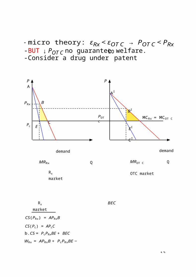
28-

Economic

s Healthof

iples

Highest premium willing to pay?

Def.: Certainty equivalent (CE). Level of income whose utility is equal to expected utility, U (CE) = E(U ).

Highest premium = E(Y ) − CE

28

�

→

*Supply of insurance

Z∗ depends on α. In turn, α is a decision of insurance company. Such decision depends on the structure of insurance market.

Assumption: perfectly competitive market.

Expected profit = premia - indemnity payments

E(B) = (1 − p)αZ − p(1 − α)Z = Z(α − p)2 set-ups:

Set-up 1: determine α (”fair premium”) solution ofE(B) = 0. Thus,

Interpretation

α = p

The fair premium is equal to the probability of falling sick. If insurer sets lower premium will incur (expected) losses. If insurer sets too a high premium will obtain (expected) extra profits new entrants offering lower premia.

Set-up 2: determine α solving maxα E(B). Solu- tion depends on the market structure.

28-

1

1

1

1

*Equilibrium of the insurance market

- Demand: [marginal benefit = marginal cost]∂Up(1 − α) 1 ∂U= α(1 − p) 1

- Supply

∂Y 1Ys

α = p

∂Y 1Yh

Therefore, p(1 − α) = α(1 − p), and market equilibrium is characterized by

∂U 1

11 =

∂U 1

11.

∂Y 1Ys ∂Y 1Yh

Equality only satisfied when Ys = Yh, i.e.

Y − L + (1 − α)Z = Y − αZ,orZ∗ = L.

The individual optimally fully insured against expected loss.

28-

Health f

Demand of insurance and healthcare demand elasticity

• D1 and D2 demands for healthcare of 2 illnesses.• Illness 2 more severe → more demand, more in-elastic.• Price of healthcare: P

� 2 scenarios: no insurance; insurance with copayment c

Higher elasticity → insurance generates higher relative welfare gain.

2

9. Contract theory

Introduction

So far, market failure → mkt power, ∆ returns, public goods, externalities.

New element of analysis: private information (asymmetric, imperfect).

What is a contract? Bilateral agreement: contracting party (principal ) delegates in contracted party (agent ) decision making.

Elements of a contract:♦ Principal: offers contract; verifiable variables♦ Agent: if accepts, performs effort for Principal.

Perfect agent: physician as perfect agent for the patient takes decisions (diagnostic, treatment) “as if” it would be the very patient taking decisions should (s)he have the same information as the physician.→ deontologic code, hypocratic oath.

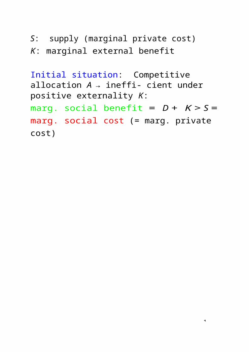
29-

- If there is no conflict, the agent behaves as if (s)he would be the principal rather than himself.- If conflict of interest, problem for the principal: make sure that the agent (physician) respects the interest of the principal (patient).- Usual scenario: conflict of interest between principal and agent.

Conflict of objectives:♠ salary: income for agent, cost for principal♠ effort: benefits principal, costly for agent

INFORMATION?Complete (perfect), incomplete (imperfect), symmetric (public), asymmetric (private)

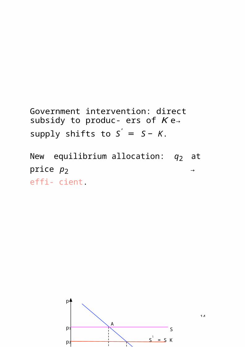
29-

Definitions

Perfect information: at each move, party knows history of decisions so far.

Imperfect information: not perfect.

Complete information: every party knows all rele- vant information about other party (parties know decision tree).

Incomplete information: ∃ party uncertain about other party’s behavior, i.e. there are random elements in the relationship.

Symmetric information: all parties have exactly the same information;

Asymmetric information: One party has more information than the other party.

29

H1b nb

H2

b nb b nb

H1b nb

H2

b nb b nb

Illustration 1: complete information

2 Hospitals deciding whether buying or not, new MRI device.

Payoff: patient share.

1/2 3/4 1/4 1/2 1/2 3/4 1/4 1/21/2 1/4 3/4 1/2 1/2 1/4 3/4 1/2

Complete and perfect information Complete and imperfect information

29-

Np 1-p

H1 H1b nb b nb

H2 H2

b nb b nb b nb b nb

Np 1-p

H1 H1b nb b nb

H2 H2

b nb b nb b nb b nb

Illustration 2: incomplete information

H1 may be aggressive (pr. p) or soft (pr. (1 − p)). Nature determines. H2 does not know attitude H1.

0.7 0.8 0.6 0.5 1/2 3/4 1/4 1/20.3 0.2 0.4 0.5 1/2 1/4 3/4 1/2

Incomplete and perfect information

0.7 0.8 0.6 0.5 1/2 3/4 1/4 1/20.3 0.2 0.4 0.5 1/2 1/4 3/4 1/2

Incomplete and imperfect information

29-

Provision of incentives and objectives in the healthcare sectorObjetive: Maximum quality with minimum cost.

PATIENTS

Problem 1:

Healthcare insurance → limited cost sensibility, excessive visits, only issue is quality.Incentives: cost-sharing (copayments). [Avoid equity issues!]

Problem 2:

Degree of precision in following treatment → hard to correct.US (1995) losses due to deviations in use of pharmaceuticals: 80,000 - 100,000 mil $

[recall efficacy vs. effectiveness (p. 6f)]

29

→

→

∇

PHYSICIANS

Problem 1:

Market of experts ”trust goods”: diagnostic and treatment.Treatment: difficult to assess its quality (subject to random elements, every patient is different, ...).Valuation can only be made by provider.

Incentives: Separation between diagnostic and treatment.Example: Japan (Macho-Stadler, I., 1999, “Reflex- iones sobre la provisioń de incentivos en los servi- cios sanitarios”, p.5)Incentives: Patient access to second opinions discipline via reputation BUT search of info is costly.

Problem 2:

“Supplier induced demand” (capacity of the physician to manipulate his income or the importance of a service)

Incentives: Patient: access to second opinions; In- surer: prices/services does not work. Ej.: Os- akidetza (Macho-Stadler, I., 1999, p.6)

29-

Definitions of types of goods under asymmetric information

- search goods: their quality is apparent before pur- chase.

- experience goods: their quality is apparent after consumption.

- trust goods: their quality is not always apparent even after consumption.

29-

Problem 3:

2 payment systems: fee-for-service, or capitation.

fee-for-service [fixed payment + cost reimbursement]: provider does not participate in costs; does not have control on costs; does not avoid difficult (costly) patients.

capitation [fixed payment per patient]: cost contention; avoids costly patients.

Incentives: combination: fixed payment + partial cost reimbursement → allows for cost control maintain- ing quality.

29

HOSPITALS

2 payment systems: prospectives or retrospective budgets.

retrospective budgets [ex-post reimbursement of costs]: no cost control.

prospective budgets [ex-ante]: cost control; quality tends to ↓, unforeseen events (epidemic episodes , catastrophic situations,...)?

Incentives: Prospective budget + payment according to comparative performance.Define “normal” price to each hospital service based on average. Exclude special treatments.

Conclusion:

No incentive mechanism adequate for all situations: Often, incentive mechanisms raise (unwanted) second order effects, BUT better than doing nothing.

29

Asymmetric info and conflict of objectives. Example

Hospital (principal) contracts manager (agent) to de- fend interests of hospital.Hospital cannot perfectly control manager’s decisions. Contract cannot be based on manager’s behavior (not verifialble).Hospital does not have info on manager’s characteristics.Manager can exploit his informative advantage to his own benefit, instead of hospital’s.

Aim: study relation between two individuals, where one of them has an informative advantage over the other and their objectives are not aligned. =⇒ Provision of incentives to reach objective.If interests would coincide, info would be communi- cated eliminating asymmetry.

3 topics: moral hazardadverse selection signalling

29

Mar

Xavier

Qc

Moral hazard

In a moral hazard situation both parties have the same info at the moment of signing the contract, BUT afterwards the agent receives private info. The principal cannot observe (verify) the effort (action) exerted by the agent.

Examples

Source: Macho-Stadler et al. (1994, p. 21)

* labor contracts: publisher representative to sell books. Only verifiable element: # books sold. Effort (# hours visiting clients) not verifiable by publisher→ payment cannot be dependent on effort.

* hospital: manager contracted to control costs. If fixed payment → insufficient effort.

* researchers: research center contracts researcher in a project. → difficult to distinguish a thinker from a dreamer. Fixed payment → little incentives to think.

29

Example 1. Hospital with retrospective budget →little incentives for cost containment Na ı̈ve solution: prospective budgets.

Example 2. Fully insured driver → little incentive for careful driving.Na¨ıve solution: “bonus-malus” system

Example 3. Fully insured physician → little incentive to exert the (costly) efficient level of effort to obtain best diagnostic.Na¨ıve solution: make physician responsible for diagnostic errors. Reputation (cf. TV series “House”)

Na¨ıve solutions because too much risk on the agent:(i) hospital may have high costs because unexpected Lo unfortunate case mix, epidemic episodes ... (and for lack of effort)(ii) driver may be unlucky on one occasion along the year.(iii) physician may obtain a wrong diagnostic by accident.

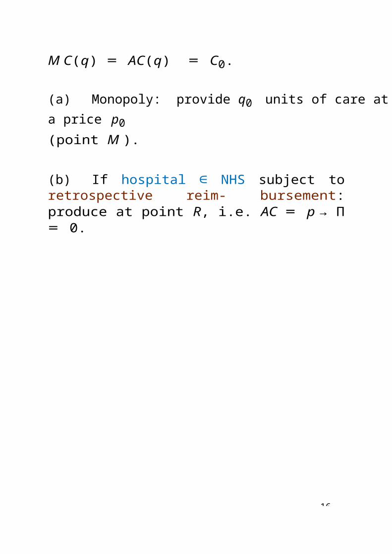
29-

Too much risk on the agent. What to do?

♠ Hospital with prospective budget. Too a high risk (earthquakes, epidemic episodes, ...)

Solution 1: Observe average performance along time and implement compensations according to deviations from the average value.

Solution 2: Induce competition among hospitals. In- direct method to achieve the same objective.

♠ Hospitals with /= case mix (because of the environment where they perform activity)

Solution:Step 1: define types of illnesses with similar cost/patient (Diagnostic related groups)Step 2: Use unit average cost for each DRG and compensate the hospital per patient within each DRG.

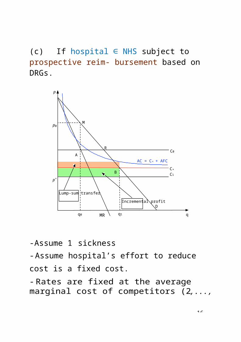
29-

→

−

→ ⇒

Moral hazard and demand for health care

Health Insurance: price patient /= price treatment

Health insurance ∆ price of health services So far: L exogenous, BUTdemand sensible to price, Z∗?

Assume (1):Prob p sick, demand for treatmentProb (1 p) healthy. No demand for health services.

We already know:contract full healthcare insurance (cost of treatmentP1Q1); premium: pP1Q1

Assume (2):Demand decreasing in pricefull healthcare insurance free treatment∆ demand for healthcare until the level P = 0, sayQ2 > Q1.

Consequence:Real cost of treatment: P1Q2 > P1Q1⇒

Problem:

29-

♠ If insurer maintains premium, expected revenuepP1Q1, expected payment pP1Q2 → losses.

♠ If insurer increases premium to pP1Q2 individual cannot contract insurance. (May buy premium> pP1Q1 as protection against risk)

Premium: 2 components- protection against risk,- supplementary resources to compensate moral hazard.

As before, Z∗ → MR=MCnow, individual costs = premium + moral hazard.

♠ Insurer’s mechanisms to provide incentives to in- surees: deductibles and copayments.

29-

Qc

Economic

s ealthof

Effect of a deductible

Assume insurance contains a deductible of D e (Cost borne by insuree before insurer starts covering expenses).Individual compares the level of services obtained after paying the deductible (Q2) and without insurance (Q1).

Example

* no insurance: (P1, Q1)* p: prob “accident”* D = P1Q1* individual obtains Q2 paying D(= P1Q1)* benefit: area under demand curve between Q2and Q1 (green area)

29-

vierM

cXa

Insurer ∆D to D, = P1Q3. Will the individual buy the insurance?

♣ ∆ payment if sick = P1(Q3 − Q1) (blue+yellow)♣ benefit: area under demand curve between Q2and Q1 (blue+green)♣ Summary:- expense increase: yellow- benefit increase: green

Conclusion:If green > yellow → contract insurance with deductible D,. Otherwise,Too high a deductible → eliminates incentives to contract insurance

29

M

Xavier

Qc

Economics

−

→

→→

Effects of a copayment

Initial situation: no insurance (P1, Q1)

Contract insurance with copayment c ∈ (0, 1) i.e.P2 = cP1 ⇒ Demand increases Q1 → Q2

Value of services = P1Q2∆ expenditure = P1(Q2 Q1) (blue+yellow)∆ benefit = area under demand curve between Q2and Q1 (blue)Triangle yellow: welfare loss Individual demandsmore insurance services than optimum.

InterpretationInsurance consumer “as if” ignorant real cost of health services distortion in resource allocation between demand for insurance and other goods.

29

XaQc

Economic

s ealth

Copayment and market equilibrium

Initial situation: no insurance (P1, Q1) with demand= supplyContract insurance with copayment c ∈ (0, 1)⇒Demand increases Q1 → Q2New equilibrium: (P2, Q2).

∆ expenditure = P2Q2−P1Q1 (blue+green+yellow)Resource allocation distortion:∆ benefit induced by copayment = green∆ costs additional demand = blueDeadweight loss from overproduction of insurance services = yellow

3

Xavier

Qc

→

Adverse selection

Adverse selection appears in situations where the agent has private information before signing the contract. In this case the principal can verify the agent’s behavior. Principal knows there are several types of agents but cannot identify it at the moment of the contract.


Examples* Insurance company may face a potential client with high or low risk. Insurer can design a contract for each type of insuree, but does not know ex-ante which is the optimal one.

* Regulation of a public monopoly. Theory: price to marginal cost and cover fixed cost with a transfer. monopoly knows better its cost function than regulator. Regulator includes monopolist informational advantge in the design of the contract (transfer, price).

30-

* Patient has better info on his real health status than insurer → excessive costs, higher probability of falling ill.

* Hospital has better info on the case mix of patients than insurer and Health authority → inflation of costs and budgets.

* Physician, after the visit, has better info on the patient’s real health status than- patient → induced demand, prescription of branded drugs (instead of generics)- hospital → excessive referral to specialized care.

30-

Asymmetric info may cause the market to perform poorly, and even disappear.

Asymmetric info, key element in insurance and health care markets.

Illustration: Akerlof’s (1970) lemons

market. Used-cars on sale with /=

qualities.Sellers know about qualities better than buyers.Lemons principle: Good cars are driven out of the market by the lemons

30

4 2 4 4 2 4

1

Simplified Akerlof’s example (FGS, 2004, ch. 9):

• 9 used-cars qualitiesq = {0, 1 , 1 , 3 , 1, 11 , 11 , 13 , 2}

• Uniform prob. of picking a car (= 9)

• Sellers know quality

• Buyers only know distr. qualities

• (min) Reservation value to sellers= 1000q e

• (max) Reservation value to buyers= 1500q e

• Auctioneer calls out market prices

• Sale at a price s.t. D = S

30-

�

Let p = 2000e per car

• Supply:Sellers willing to sell each car if for each car,p ≥ 1000 × q.

car (q=2)→ 2000 = 1000 × 2 → S=9.

• Demand: Average quality=1;Buyers willing to buy if p ≤ 1500 × 1 =

1500; (price)2000 > 1500(res.value) → D

= 0.

30-

�

�

�

�

4


• Supply:Sellers willing to sell each car if for each car,p� ≥ 1000 × q.

pq=2 = (1000)2 = 2000 > 1500 → not offeredpq=1.75 = (1000)1.75 = 1750 > 1500 → notofferedpq=1.5 = (1000)1.5 = 1500 = 1500 → offeredpq=1.25 = (1000)1.25 = 1250 < 1500 → of-feredThus, → S=7 cars; average quality = 3/4.

• Demand:Average quality q¯ = 3/4;Buyers willing to buy if pq¯ ≤ 1500 × 3 = 1125.Thus, (price)1500 > 1125(res.value) → D = 0.

etc, etc.

Conclusion:Under asymmetric info, �p at which D = S.

Why? Lemons principle.

30

Assume symmetric info:

Buyers and sellers only know average quality (q¯ = 1).


• Supply:Sellers willing to sell if pq¯ ≥ 1000q¯ = 1000;

(price)2000 > 1000(re

�s.value) → S = 9.

• Demand:Average quality q¯ = 1;Buyers willing to buy if pq¯ ≤ 1500q¯ = 1500;

(price)1500 = 1500(res.value) → D = 9.

Equilibrium price of 1500 e and 9 cars are sold.

30-

Akerlof and health insurance market.

Individual has more info on his real health status than insurer.

If insurer ignores this fact, and set premium according to general population statistics → losses. Why?- high risk individuals more interested in contractinginsurance →- insurer’s customers will be a biased population sample.

Insurers anticipates it → contracts with higher premia. Low risk individuals do not contract insurance: Exclusion

Conclusion: asymmetric info → inefficient resource allocation.* ind. do not know their p → insurance against risk.* If insurer offers same contract to everybody →- low risk indiv, too high premium → underinsurance- high risk indiv, too low premium → overinsurance.

Solutions

30-

Solution 1: Screening

Insurer offers menu of contracts:- i) contract with high coverage and high premium;- ii) contract with low coverage and low premium

Consequence: self-selection:- low risk indiv, → contract ii)- high risk indiv, → contract i).

Problems1. Argument OK if insurer is monopolist. / ∃ eq. if competition.2. Even when ∃ eq, it is inefficient: low risk indiv. overinsured.

Solution 2: Signaling

3

Qc

Economics

Signaling

Similar situation to adverse selection. After knowing his type and before signing the contract, the agent may send a signal observable by the principal.


Example

* Physician shows credentials (Ph.D., etc) as signal of ability when being contracted by hospital/patient. Also hangs from the walls of his office credentials so that patients can see them.

31-

Mar

Xavier

Qc

Alternatively, the principal may posses private info that transmits to the agent through the contract design.


Example

* University Dpts in job market include “goodies” in offers as signals of quality.

What is a signal? investment to disclose some info (the “type”) yielding some advantage over keeping it secret.

31-

Solution 2: Signaling

Low risk indiv. willing to show to insurer they are low risk:e.g. volunteer medical reports.⇒ Signaling theory

Problemhigh risk indiv. want to look like low risk imitating their signals.

Consequence- Insurers very cautions in interpreting signals- As signaling is costly, low risk indiv. may prefer not to signal.

Equilibria: 2 types(i) Separating equilibrium(ii) Pooling equilibrium

31

→

→

(i) Separating equilibrium

Appears when signaling is very costly for high risk indiv.- high risk indiv. do not imitate- Insurer takes signals serously- low risk indiv. obtain better contracts- signaling attractive for low risk indiv.

(ii) Pooling equilibrium

Appears when imitation is not very costly- Insurer ignores signals- Signals are useless- Nobody signals

Problem (technical, but important)

Even with high signaling costs, often also exist pooling equilibria.

Examples:- Corporation places ad looking for “young graduate”

education as a signal of ability.- Hospital real “case mix” difficult to know by Healthauthority.- Physicians’ ability hard to know by patient.

→

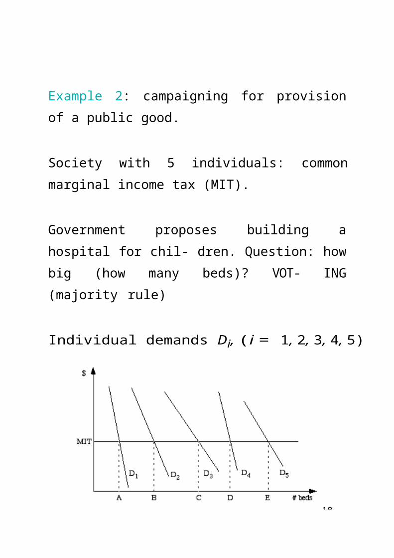
31-

Summary

Asymmetric Info gives rise to the possibility of ask- ing the following questions:

◆ A situation with relatively ignorant consumers pre- vents high levels of competition?◆ Should be observe high price dispersion in the health care market?◆ Will the health care market provide unnecessary or non optimal treatments to patients?

Objetive: find mechanisms to correct for the bad consequences of asymmetric info.Incentive contracts, competition, ...

BUT

Contracts require verifiable info → costly (monitoring, auditing)

Competition may lead to exclusion of some groups of individuals → equity, social justice

31-

Reading

The Henry J, Kaiser Family Foundation, 2006, Illus- trating the Potential Impacts of Adverse Selection on Health Insurance Costs in Consumer Choice Mod- els, Snapshots: Health Care Costs,

http://www.kff.org/insurance/snapshot/chcm111006oth2.cfm

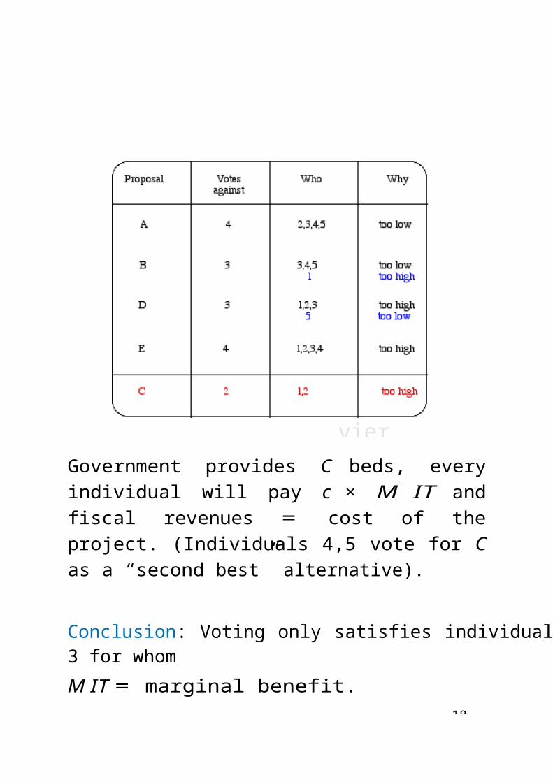
3

Supplier induced demand

WHAT IS IT?Agency problem. Patient’s dependency on physician gives physician an advantage (due to better info) to manipulate demand to his benefit.

Old topic (1958 →) Roemer’s effect: “a bed built is a bed filled” (Roemer 1961) Very high correlation between availability of beds/1000 inhabitants and occupation rate (days in hospital/1000 inhabitants).

Generalization to physician services → SIDWell documented phenomenon, although controversial- introduction of wages controls on physicians, often∆ SID- clinical decisions often influenced by financial incentives (e.g. physicians with salaries, lower hospitalization rates then physicians payed on fee-for- services basis).

32-

Mart

Xavier

Qc

Basic model of SID

Initial situation (P1, Q1). Supply increase S1 → S2

Standard micro analysis: eq: (P2, Q2). Total expenditure Lo o y according to ε.Healthcare services: ε < 1 → Total expenditure ↓Moreover, Lo � physicians → lower demand/physician.

SID: physicians use their capacity to induce extra demand (D2). New eq. (P3, Q3).If P3 > P1 SID with certainty (Reinhardt induce-ment test).If P3 < P1 ambiguity.

Modeling problem: analysis assumes competitive market.

Mar

Xavier

Qc

Economics

→

Other models of SID

1. Evans (1974) model

(simplified) Physician’s utility: U

(Y, D)Y = income; D = inducement ( � h. induced demand)

Assume: π average profit rate- max profit without inducement: πQ0- profit from inducement: πDTherefore: Y= πQ0+πD combinations (Y, D)feasible for physician.Given U , eq. in A = (YA, DA)* If Lo competition: π → π,, π, < π →New eq. with Lo

,inducement: DA → DB

aiming at π,Q0 + π,D, ≥ πQ0 +

πD. 32-b

32

2. SID vs. advertising

Begin: max. profit → M R1 = M C1 → (P1, Q1)

P

P2MC2

P1MC1

D1

Q1 Q2

MR1

D2

Q

MR2

Margin (P − CM ) incentive to stimulate demand as each additional unit yields profits: D1 → D2 ∼ argument to introduce advertising.

BUT

inducing demand has cost (reputation, time): M C1 →M C2New equilibrium: (P2, Q2)

32-

Remarks1. Incentives to induce demand depends on the difference between P and M C (market power)- if competitive market, small gap, low incentives;- if high market power, big gap, high incentives- empirical evidence: physician, high monopoly power.

Enhance competition to limit incentive to induce demand.

2. Professional and ethical considerations limit physicians activities (contracts between principal (patient) and agent (physician)) → limits informational advantage:- monitor insurer activity- ease possibility of second opinions- improve patient’s info on treatments (internet)

3. Distinction between informative advertising (positive) and persuasive advertising (negative) corre- sponds to a physician transmitting info to the patient (positive) or implementing non optimal/unnecessary treatments (negative).

3

10. Economic Evaluation

Optimal policy design requires evaluation to select best alternative:

• What is included in the estimation of costs: the costs at the hospital, the social costs, cost to the individual?

• We assign value to commodities through our choices on the (free) “market-place”. But most markets are neither free, nor ideal. To consent in a market is not identical to consent to a market. Can these considerations be included in the analysis? How?

• Can we put a price on everything? is everything a commodity that is for sale if only the price is right? life, honor, rights, embryos, human tissues...if not, there are certain things that will be difficult or im- possible to include in the economic analysis.

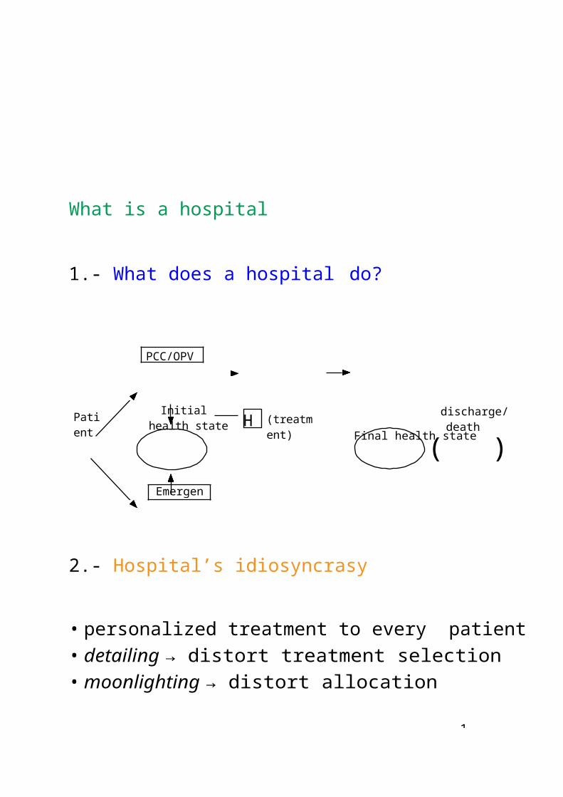
33-

τ =1

General difficulty: assign value to human life

Quality-Adjusted Life Years (QALYs)

Most often used measure of health services.

- Consider an individual with health status Qt in yeart and life horizon T .- Ideal health state is Q∗ (reference value)- Let H(Q) be utility of individual with Q- (Q1, t1; Q2, t2; . . . ; Qn, tn) health profile. Qτ pre-vails tτ years,

),n tτ = T- r discount rate (interest rate)

33-

Definition: QALY

QALY index is a measure of the utility of health status, U (Q, T ), defined as the present value of the utility of each health status weighted by the time period along which that health status prevails:

nU (Q1, t1; Q2, t2; . . . ; Qn, tn) = Qτ tτ

τ =1 (1 + r)τ

Weight =1 if perfect health status. Weight = 0 if death (negative as well)

Example 1Indiv. 70 years old, life expectancy 20 more years. First 10 years, perfect health (weight = 1),Second 10 years, half quality of life.QALY = (10 × 1) + (10 × 0.5) = 15.

33

Example 2: Esclerosis mu´ ltipleNiveles de incapacidad:

1. Ausencia de incapacidad.

2. Ligera incapacidad social.

3. Incapacidad social grave y/o ligero deterioro del

rendimiento laboral. Capaz de realizar todas las tareas

dome´sticas excepto las muy pesadas.

4. Limitacioń muy grave en las posibilidades de eleccioń

de trabajo y en el rendimiento laboral. Las amas de casa y

los ancianos son tan solo capaces de realizar tareas dome

´sticas ligeras, pero son capaces de ir de compras.

5. Incapacidad para conseguir un empleo remunerado. Inca-

pacidad para proseguir cualquier tipo de educacioń.

Ancianos confinados en su hogar, excepto raras salidas

acompanãdas y breves paseos, e incapaces de ir de

compras. Amas de casa capaces so´ lo de realizar unas

pocas tareas sencillas.

6. Confinado en una silla de ruedas, o bien incapaz de des-

plazarse por la vivienda sin la ayuda de otra persona.

7. Confinado en cama.

8. Inconsciente.

33-

Incapacidad Niveles de sufrimientoAusente Leve Moderado Grave

Nivel 1. 1.000 0.995 0.990 0.967Nivel 2. 0.990 0.986 0.973 0.932Nivel 3. 0.980 0.972 0.956 0.912Nivel 4. 0.964 0.956 0.942 0.870Nivel 5. 0.946 0.935 0.900 0.700Nivel 6. 0.875 0.845 0.680 0.000Nivel 7. 0.677 0.564 0.000 -1.486Nivel 8. -1.028 na na na

Veáse Hidalgo, A. (2000): Evaluacioń econo´mica de

tecnolog´ıas sanitarias, en Hidalgo et al. (2000, cap. 12).

33-

Historia de un paciente:- Sano durante 28 anõs- Primeros s´ıntomas: 29 anõs- Empeoramiento progresivo- Muerte: 49 anõs.

Edad Incapacidad Sufrimiento Indice Valor0-28 Sano Ausente 1.000 28.00029 nivel 2 Leve 0.986 0.98630-33 nivel 2 Moderado 0.973 3.89234-36 nivel 3 Moderado 0.956 2.86837-40 nivel 4 Moderado 0.942 3.76841-43 nivel 5 Grave 0.700 2.10044-46 nivel 6 Grave 0.000 0.00047-49 nivel 7 Grave -1.486 -4.458

QALY 37.156

QALY = (28 ∗ 1) + (1 ∗ 0.986) + (4 ∗ 0.973)++ (3 ∗ 0.956) + (4 ∗ 0.942) + (3 ∗ 0.7)++ (3 ∗ 0) + (3 ∗ −1.486) = 37.156.

QALYs < 49 anõs: calidad de vida desde la aparicioń de los s´ıntomas va en continuo retroceso.

33

→→

Example 3. Eval. alternative health programsPatient with health status 60% optimal. If medication 3 more years alive.If surgery 5 more years and better quality of life. Success rate of surgery: 40%.Prob. dying in surgery room: 3% Cost of surgery = 30, 000 e Discount rate = 5%

QALYs: Medic.= 1.44 QALYs; surgery = 3.23 QALYs Risk of death w/ surgery = 3.23 × 0.03 = 0.09 Expected net ∆ QALY = [(3.23 − 1.44) × 0.4] − 0.09 = 0.72 − 0.09 = 0.63 QALYi.e. surgery → expected net ∆ QALY = 0.63

Cost per extra QALY = 30, 000/0.63 = 47, 620 e

Conclusioń: Patient if surgery, expected ∆ QALY of0.63 years, at a cost of 47,620 e per QALY.

Year 1 2 3 4 5 totalDiscount 1.00 0.95 0.91 0.86 0.82MedicationLife quality Disc. value

.60

.60.50.48

.40

.36.00.00

.00

.00 1.44SurgeryLife quality Disc. value

.90

.90.80.76

.70

.63.60.52

.50

.41 3.23

33-

45º

M

↓Lo →

y

Ejemplo 3. Resource allocation Society: 2 individuals, A, B Initial situation: A1 = B1, (M )Society gets extra resources → ∆ health →R = max(A∗ + B∗) s.t. (A∗, B∗) ∈ health frontier

B’s QALYs

BmaxB*

B1

N

Q U

Health frontier

0 A1 A*

Amax

A’s QALYs

From R and along the frontier, A’s QALY B’s QALY s.t. A + BIs R socially efficient and/or egalitarian?As Bmax > Amax, the same resources will yield more QALYs to B than to A.Given that R = max(A∗ + B∗), R is socially efficient but, not egalitarian (B∗ > A∗).Egalitarian allocation: Q

R

34-

Allocation max social welfare: N (not egalitarian)

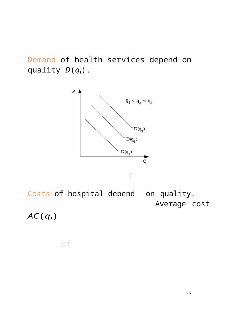
3

Economic Evaluation Questions for a planner:♠ Who should do what to whom?♠ With what health care resources?♠ With what relation to other health services?

Replies (Definition: Economic evaluation) Comparative analysis of the use of resources (costs) and improvements from alternat.health programs (consequences).

Issues to analyze,Efficacy: Can the program work?

Effectiveness: Does it work?Data: medical literature; but consider- should adjustments be made?- quality? Question checklist (McMaster Univ, ’81)- relevance?

Availability: Does it reach the target population ?

Opportunity cost: is it worth compared with alternative uses of the same resources?

Optimality: Best possible use of resources?

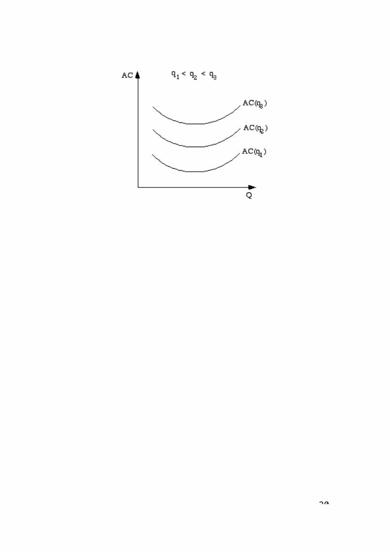
alt

tinez-Gir Mar

X

avier

Qc

3

Components in Economic Evaluation

Consequences: 3 categories- Identification: Health effects (e) (Lo QALYs)- Valuation: utility (u), monetary (w), “info” (v)- Measurement (s): resources saved (s1, s2, s3)

Costs- health care sector (c1): hosp, physicians, pharma- patient/family (c2): income, time- other sectors (c3): opportunity costs

−

−

−

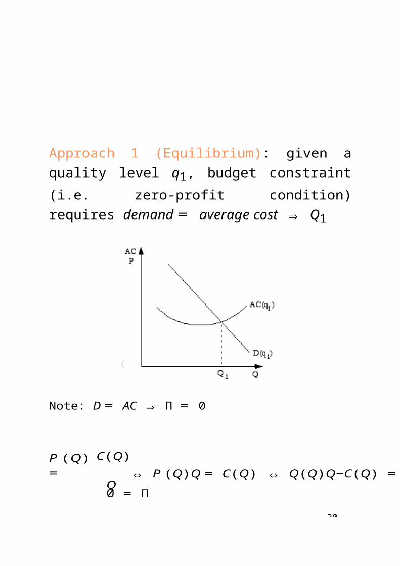
3

Economic Evaluation Techniques Combination of costs and consequences

COMPARISON OF COSTS AND CONSEQUENCES

A L T E R N A T I V E S

Cost minimization analysis(c1 + c2 + c3) (s1 + s2 + s3) Cost-effectiveness analysis (CEA) [(c1 + c2 + c3) (s1 + s2 + s3)]/e Cost-utility analysis (CUA)[(c1 + c2 + c3) (s1 + s2 + s3)]/uCost-benefit analysis (CBA)(w + v + s1 + s2 + s3) − (c1 + c2 + c3)

NO YES

N O

ONLY COSTS ONLY CONSEQUENCES

COST-OUTCOME DESCRIPTION

COST DESCRIPTION

OUTCOME DESCRIPTION

Y E S

EFFICACY COST-MINIMIZATIONCOST OR COST-EFECTIVENESS

ANALYSIS EFFECTIVENESS COST-UTILITY

EVALUATION COST-BENEFIT

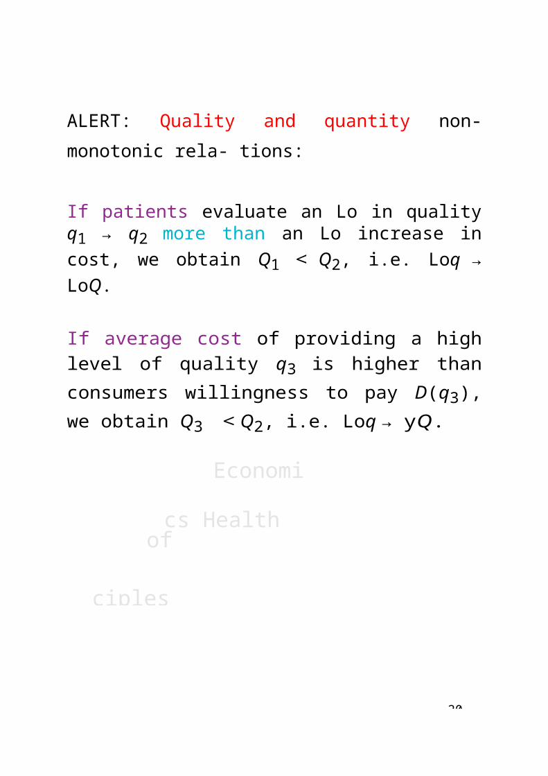
3

Measurement of costs consequences

MEASUREMENT OF COSTS AND CONSEQUENCESTYPE OF STUDY

MEASUREMENT / VAL. OF COSTS

IDENTIFICATION OF CONSEQUENCES

MEASUREMENT / VAL. OF CONSEQUENCES

Min Cost $ IDENTICAL NONE

SINGLE EFFECT OFCEA $ INTEREST COMMON

TO ALL THENATURAL UNITS /

NONEALTERNATIVES

CUA $ SINGLE OR MULTIPLE EFFECTS

QALYs / COST per QUALY

NOT NECESSARILY

CBA $ $COMMON TO ALL THEALTERNATIVES

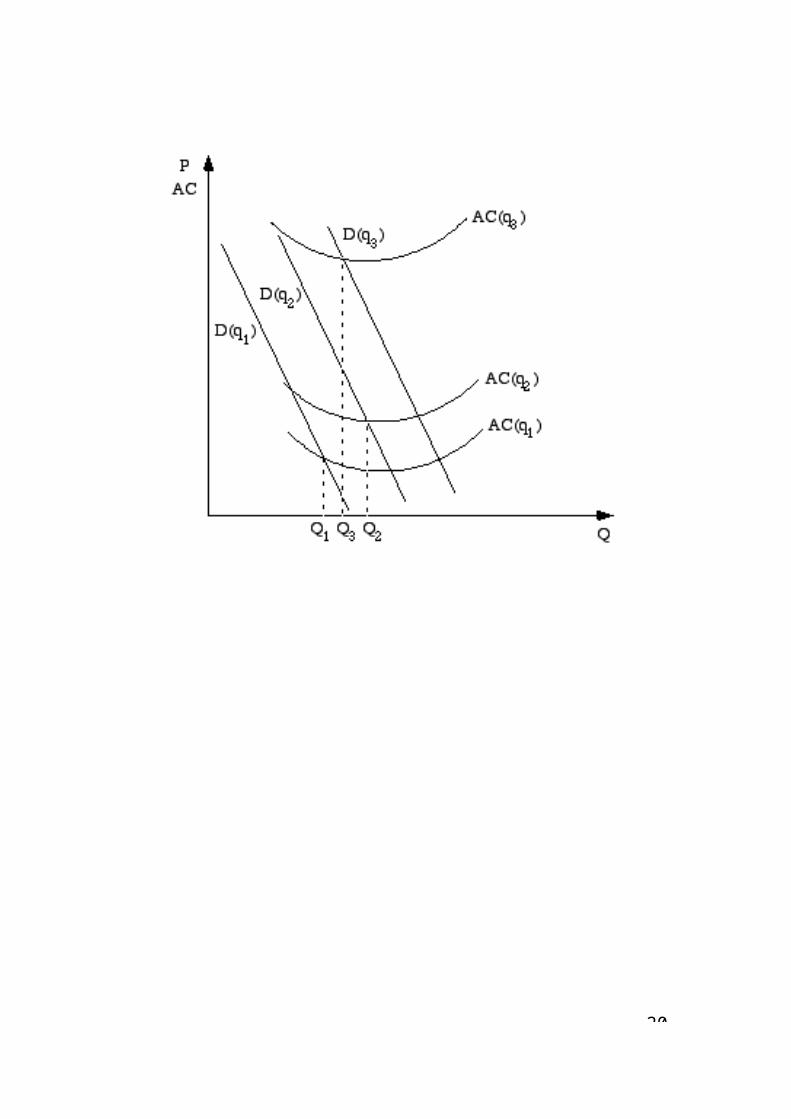
3

Cost minimization analysis

Illustration 1

2 programs: minor surgery for adults

Both accomplish successful surgery

Differ in effectiveness:A: one night stay in hospital B: day-surgery program

Evaluation: select the least cost alternative.

38-

Cost minimization analysis (2)

Analysis: Four basic questions:

1. What costs should be considered?

♠ Health care sector♦ Hospital resources (treatment, bed days, out-patientattendance, overheads)♦ Community care resources (GP visits, nurse visits, ambulance)

♠ Patient and family♦ Patients time: treatment and off-work♦ Time of relatives looking after the patient♦ Out-of pocket expenses

♠ Other sectors♦ social workers visits, nursing home help, volun-tary sector

38-

♠

♠

2. What costs should be included?

Viewpoint of analysis.health sector?, hospital’s?, patient’s?, social?e.g. monetary compensation while off-work:♦ socially: no cost, no benefit (transfer)♦ Government: cost♦ Patient: revenue.

♠ Short/long run evaluation.♦ Intertemporal prefs (life is short, future uncertain)♦ Illustration

Year Cost A Cost B1 5 152 10 103 15 4

Total 30 29

♠ Justify exclusion of “irrelevant costs”.

♠ Order of magnitude.

♠ Opportunity costs.

No-market goods and services. (volunteer time, donations)

38

3. How costs should be estimated?

♠ Is there a market?YES: Opportunity costs (if there is info); Quantities and pricesNO: negotiations; market values as proxy; shadow prices. (Ethical values!)

♠ Time span of project♦ costs ↓ in hospital but out-patient treatment needed♦ costs ↑ in hospital but final (see previous exam-ple)

♠ AssetsEquipment, buildings, land...

♠ Average vs Marginal costs

Compute present values

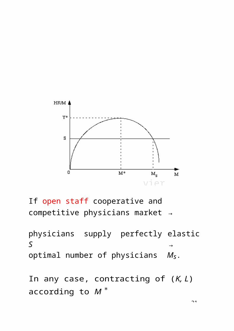
38-

Discounting future costs to present values(recall example page 35b)

N

where,

P =n=1

Fn(1 + r)−n

P : present valueFn: future cost at year nr : annual interest (discount) rateTake r = 5%.P A = 26.79 < P B = 26.81 !!Note: expenses computed at the end of period.

Choice of r: praxis {0, 3%, 5%} social opportunity costsocial rate of time preference convention: 5%shadow-price of capital:3%

38-

4. How accurate does costing should be?

♠ Availability of data

♠ Time and effort vs. outcome

“Do not make the perfect the enemy of the merely good”

38

− −−

h(x,y)

f(x,y)=m

Feasibleset

g(x,y)

Shadow prices

Concept linked to optimization problem:

max f (x, y) s.a

g(x, y) < k

x,y h(x, y) < q

max L(x, y) = f (x, y)+λ(k g(x, y))+µ(q h(x y))x,y

Illustration

f (x, y): number of patients treatedx: available equipmenty: labork: budget constraintq: available time

y

38

x

38-

λ and µ represent rate of change of f (x, y) wrt change in k and q;λ and µ represent additional resources needed so that objective function achieves value beyond m;λ and µ evaluate that cost;λ and µ called shadow prices

λ > 0 ; constraint g(x, y) < k binding.µ > 0 : constraint h(x, y) < q binding.

λ = 0 ; constraint g(x, y) ≤ k not binding.µ = 0 : constraint h(x, y) ≤ q not binding →resource requirement ≤ availability

38-

−∂L

−

Example

Recall example in pp. 5i-5j.

First order conditions,

= αxα−1yβ λPx = 0 (8)∂x

= βyβ−1xα λPy = 0∂y∂L

∂λ = m − xPx + yPy = 0

Substituting values of

x(Px, m) =

y(Py, m) =

in, say, (8) we obtain

αm Px(α +

β)βm

Py(α + β)

( αm

\α−1( β m

\β

αxα 1yβ αλ = =

Px

Px(α+β)

Px

Py(α+β)

If α = 1/3, β = 2/3, m = 30, Px = 2, Py = 1,

−

∂L

38-

3

(20 \2/3

λ =6(5)2/3 ≈ 0.202

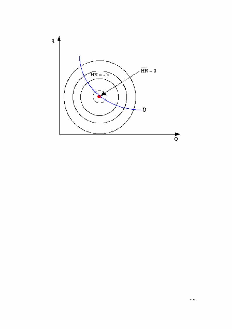
3

Cost-Effectiveness Analysis

Illustration

♣ 2 programs:- A: hospital dialysis- B: kidney transplantation

♣ Outcome of interest (common): life-years gained after renal failure.

♣ Programs Differ in success and in cost.

♣ Comparison:- Cost per life-year gained- Life-years gained per dollar spent

39-

0

♦♦

♦

♦

Cost-Effectiveness Analysis (2)

Basic elementsChoosing a measure of effectiveness define, first, objectives of the program performance of program in actual use relate tofinal health output (life-years gained) intermediate output (cases found, patients appro-

priately treated) if value by itself

♠ Linking intermediate and final outcomes♦ important in prevention studies♦ confident in proper link (previous research)

Discounting of effects (as well as costs)if only costs, may yield nonsense conclusionsif only costs, present value of the cost next year

is always lower than todayif only costs, differential treatment with respect to

other sectors in the economy may yield inconsisten- cies in the overall allocation of resources

individuals can trade reductions in health status and other goods/services today in return for a healthier time in the future (and vice versa)

0♦♦♦♠

♠

39-

♠ Uncertainties and Sensibility Analysis♦ no data may be available → “informed guess”♦ estimates may not be precise♦ methodological controversies♦ Sensibility: 3 steps0 identify uncertain parameters for which sensitivityanalysis is required0 specify plausible range of these parameters0 compute results based on best, optimistic andpessimistic guesses

Use of Quality-Life Scales

♠ Additional measure of effectiveness♠Relative costs of treatments compared with theirrelative consequences in natural units (success of therapy, life-years gained)♠ 2 types of quality-life scales♦ specific (disease specific, age specific)♦ general health profiles: Short Form 36, Notting-ham Health Profile, Sickness Impact Profile

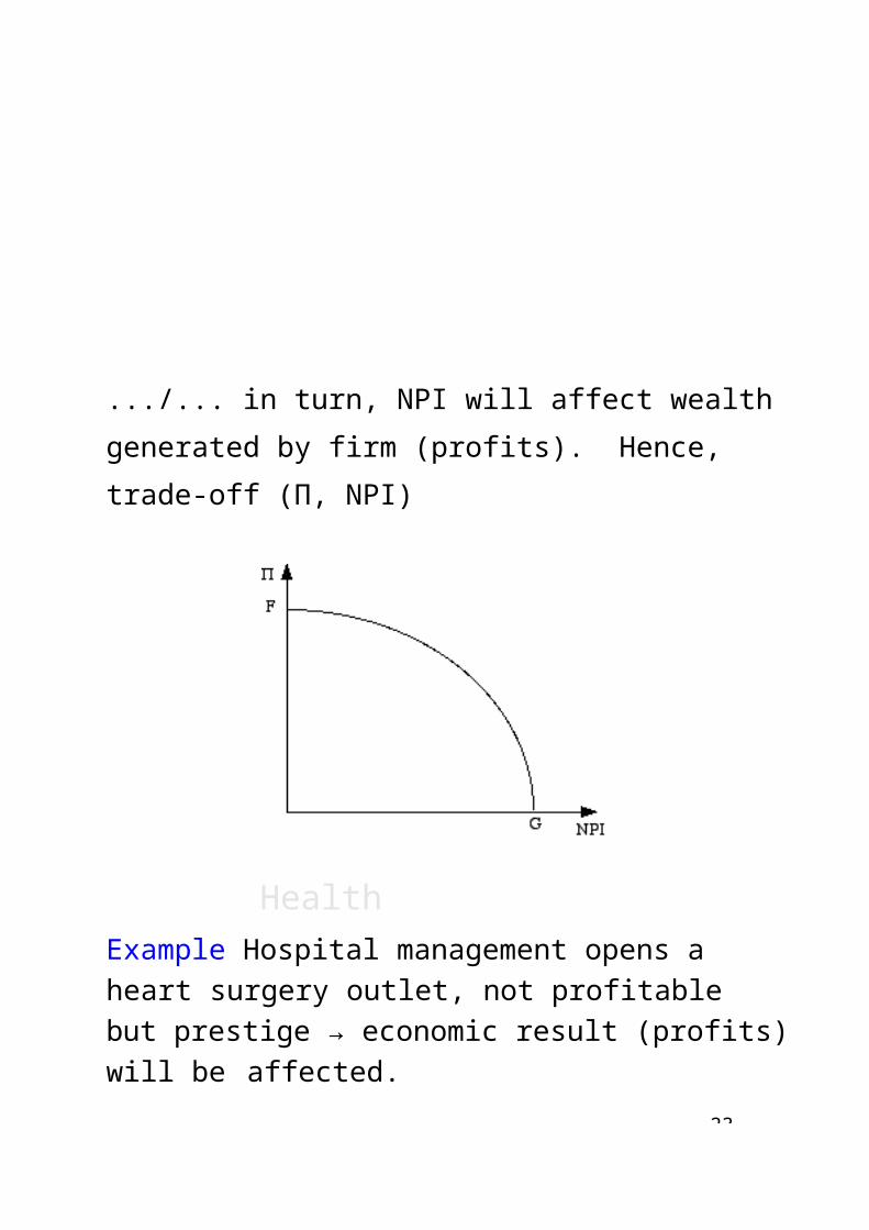
39

General health profiles

0 physical functioning 0 ability for self-care 0 psychological status0 level of pain and distress0 social integration

Advantages:reliable and valid, supplementary information only.

Disadvantages:- multidimensional- not based on individuals preferences- not possible to combine quality and quantity of life

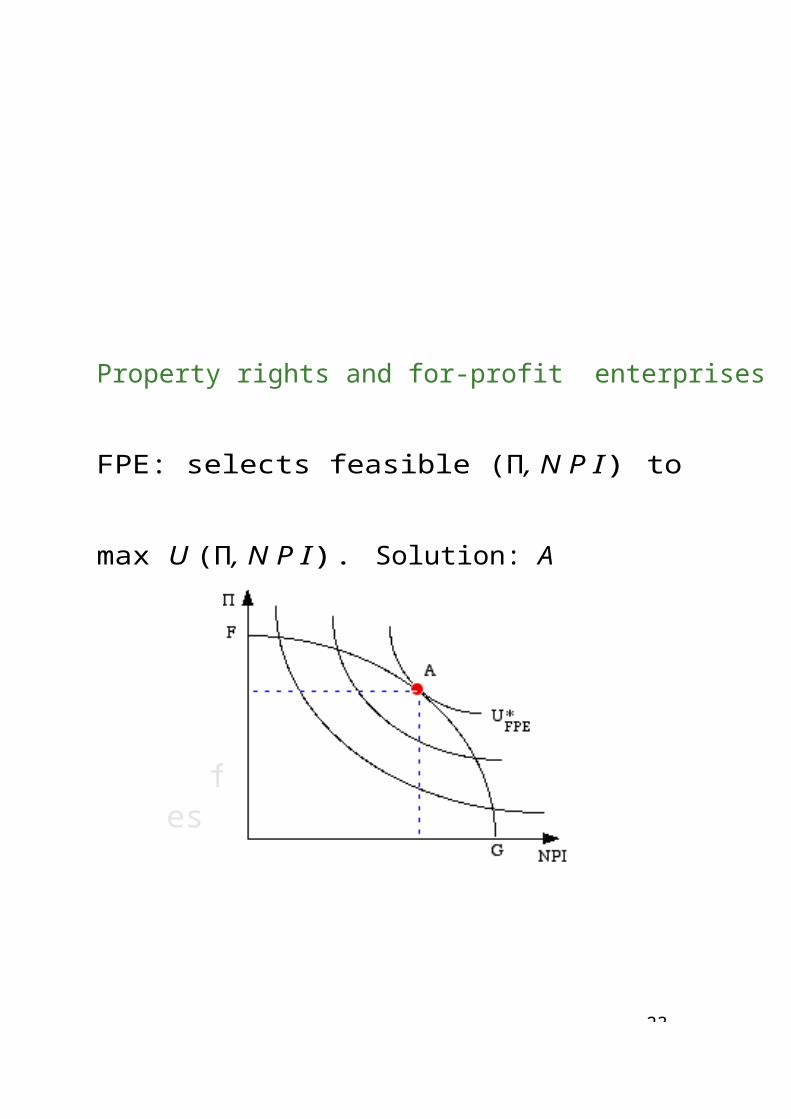
4

Cost-Utility Analysis

Illustration

♠ Measure of value: utility of effects.

♠ Twins identical except in occupation (sign painter, soccer player).

♠ Valuation in [0,1] of broken arm will differ

♠ Utility of treatment will differ

♠ CUA allows for quality of life adjustments via QALYs: generic outcome measure for comparison of costs and outcomes in different programs.

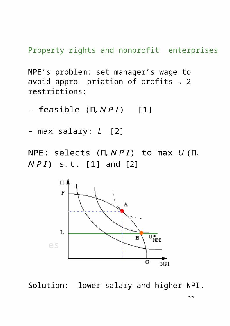
40-

Cost-Utility Analysis (2)

Basic elements

♠ Form of evaluation that places particular attentionon the quality of the health outcome produced.♠ CUA vs. CEA♦ CEA: evaluation measured in natural units (bloodpressure improvement, patients improved, lives saved, life-years gained, etc.)♦ CUA: measured in QALYs gained.♦ Identical on the cost side. Different on the out-come side (see p.33)♦ CEA: its specificity makes comparisons across studies difficult.s♦ CUA: generic measure of outcome allows for comparisons. Highlights crucial role of preferences (utilities) in valuing the outcomes.♠ CUA is useful if:♦ health-related quality of life is important,♦ program affects both mortality and morbidity,♦ program to be compared are multidimensional.

40-

Utility function (von Neumann-Morgenstern)

♠ Utilities ≡ Preferences:

♦ Ordinal: ranking♦ Cardinal: numbers representing strength of pref-erences for the outcome relative to the others.

♠ Environment:

♦ Certainty♦ Uncertainty: risk aversion, risk neutrality, risk love

40

♠

♠

tw

p

1 p

state i for t years

Measuring preferences:ask subjects to rank health outcomes, i.e. construct a rating scale.

Interpretation: ‘The difference in desirability be- een outcomes A and B is twice as great as

the difference between C and D. Hence, I will make the

interval between A and B twice as large”.

Example:Standard gamble (classical method to measure cardinal preferences)

healthy for t years (u1)

death(u2)

(u1 > u2 > u3)

with certainty (u3)

Problem: find p such that the individual is indifferent between both alternatives.

Probability p = u 2 − u 3 : cardinal utility index.u1−u3

♠ QALYs (see pp. 30a-30d)

4

Cost-Benefit Analysis

Example 1 (multiple common effects)♣ 3 programs:- A: hospital dialysis- B: kidney transplantation- C: home dialysis

♣ Outcomes of interest (common):- Life-years gained- Quality of Life- Incidence of Medical Complications

♠ Compute cost effectiveness ratios

♠ NO alternative superior on 3 dimensions?♦ Determine a primary effect and CEA, or♦ Attach a money measure of value to all effectsresulting from each program

♠ Pro: directly comparable w/ costs

♠ Con: difficult to translate effects into e

41-

Example 2 (multiple not common effects)

♣ 2 programs:

- A: hypertension screening

- B: influenza inmunization

♣ Outcomes of interest:

- A: prevention of premature death

- B: prevention disability days

41-

Cost-Benefit Analysis (2): Measuring benefits

2 alternatives

♠ Human capital approach

♦ Use monetary value of lost productivity

♦ Problem: how to measure benefits at retirement age? It is not acceptable that there are no benefits! (cynical view: pensions saved)

♠ Willingness to pay

♦ Closer to the notion of opportunity cost

♦ More difficult to measure (but this an implementation argument)

41-

Basic open issues

0 Are ethical, cultural values pre-determined? Or do they interact?

0 What is the meaning of “fair” and “just”?No definite answer is available; it influences the way we want to measure benefits

0 include distribution concerns?Requires detailed information, presumably difficult to obtainOn conceptual grounds, offers no problem Example:

where

SW = w(y)B(y)dF (y)

- F (y): cumulative distribution of income- B(y): benefits- w(y): weight to each income level

4

Distribution concerns

♣ Usually economic evaluation does not treat ex- plicitly the distribution of consequences and costs

♣ Options made have implicit treatment:

- Willingness to pay (richer more willing to pay), gives more weight to rich people

- QALYs: same weight to everyone

4

Additional remarks

♣ Economic evaluation assumes that freed resources are redeployed efficiently.

♣ Incentives: patients with kidney problems following their treatment correctly (incorrectly)

→ are the ones with least (most) transplantations.

⇒ Bad behavior yields more severe health status and go first in the waiting list.

♣ BUT if we aim at maximize the aggregate life years, may be OK!

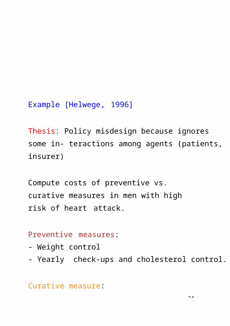
4

11. Macroeconomics

What is Macroeconomics about?

Global behavior of the economy. Aggregation.

Macro variables: GDP, Aggregate expenditure, Un- employment, Inflation, Consumption, Saving, Invest- ment, Exports, Imports, Public expenditure, etc.

Questions:

Long term growth,

Economic cycles,

Unemployment,

Inflation,

International Trade and Development,

Economic Policy (monetary, fiscal, labor, etc).

4

Definition of GDP: market value of all final goods and services produced within a country in a given period of time. [“Gross” means depreciation of capital stock included]

Measures of GDP: Two approaches: expenditure and income (equivalent)

GDP - expenditure: adding up expenditure on all final goods and services produced during the year.

GDP = private consumption + investment+ government spending + (exports - imports)

≡ C + G + I + (X − M )

GDP - income: adding up all payments to owners of resources used to produce output during the year (aggregate income)

GDP = W + P + (T − S)

Equivalence in the National Income Accounts,

W +P +(T −S) = GDP = C +G+I +(X −M )

45-

Private consumption (C): commodities and services acquired by households.

Investment (I): goods and services increasing the capital stock. Investment = Savings.

Public consumption (G): goods and services acquired by the public administrations (army, roads). No transfers (pensions, social programs) because these are transfers.

Net exports (X-M): net spending from rest of the world in goods and services yielding income to national producers.

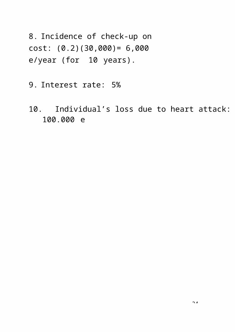
45-

Wages and salaries (W): Compensation of employees measures the total remuneration to employees for work done. It includes wages and salaries, as well as employer contributions to social security and other such programs.

Profits (P): Surplus due to owners of incorporated businesses. Often called profits.

Net taxes (T-S): Difference between the resources transferred from the families to the State and the transfers from the State to the families.

45

Illustration:

real GDP components in Spain in 2006 (constant prices 2000)Demand components

106 e %Private consumption (C) 553.867 56.7Public consumption (G) 184.233 18.9Investment (I) 298.362 30.6Exports 254.985 26.1ImportsNet exports (X-M)

315.258-60.273

-32.3

TOTAL 976.189 100

Source: Contabilidad Nacional de Espanã, INE.

45-

Illustration (2):

real GDP components in Spain in 2006 (constant prices 2000)Supply components

106 e %Agriculture 27.199 2.8Industry 151.709 15.5Construction 106.437 10.9Services 583.773 59.8Net taxes 107071 11.0TOTAL 976.189 100

Source: Contabilidad Nacional de Espanã, INE.

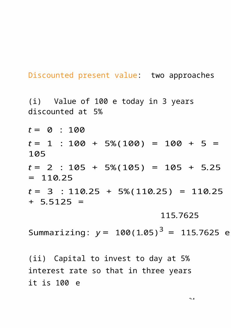
45-

8C+I

6

79

Financialmarkets

5 10

Firms

4 1

2

3

Rest of the World

Households

Government

Circular flow model:Flow of resources, products, income, and revenue among economic decision makers.

45

Legend:

Flows of income:

(1): GDP = Aggregate income.(2): Taxes are transfers from families to the State. (3): Transfers from the State to the families.(4): Disposable income of families = Aggregate income- taxes+transfers.

Flows of expenses:

(5): Disposable income splits in consumption and savings (= investment).(6): Investment adds to flow of expenditure.(7): Public expenditure adds to flow of expenditure. (8): Exports add to flow of expenditure from the rest of the world.(9): Imports are transfers to the rest of the world. (10): National account identity.

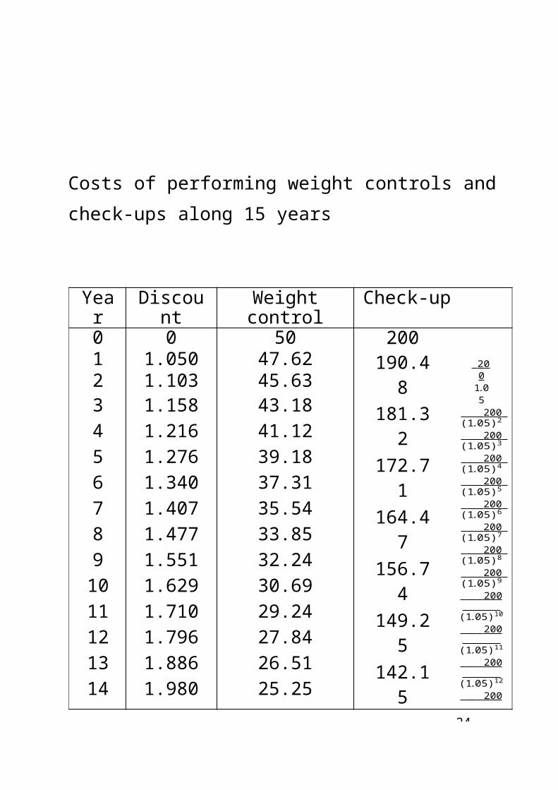
45-

Example

Orange Inc.

Wages and salaries Taxes

150005000

Juice Inc.

Wages and salaries TaxesPurchase of oranges

100002000

25000

Revenues from oranges ConsumersJuice Inc.

350001000025000

Revenues from juice 40000

Profits before taxes Profits after taxes

2000015000

Profits before taxes Profits after taxes

50003000

VA Orange Inc. = 35000 (revenues from oranges)

VA Juice Inc. = 40000 - 25000 = 15000 (revenues from juice - cost of oranges)

VA total= 35000 + 15000 = 50000 = GDP (produc-tion)

GDP (income): 10000 + 40000 = 50000 (consumers expenditure)

GDP (income): (15000 + 10000) + (20000 + 5000)=50000 (wages + profits before taxes)

Total production = Total income = Total expenditure

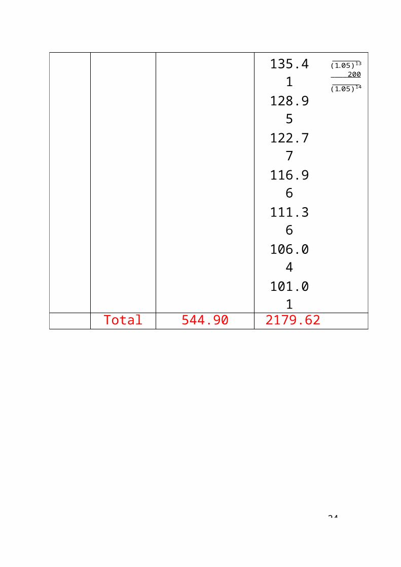
45-

ora ora app app

ora ora app app

real GDP and nominal GDP.

nominal GDP: market value of production at today’s prices.

Example: Economy with two goods (apples and oranges)

GDP n2006 = (P 2006∗Q2006)+(P 2006∗Q2006)

Problem: If prices double, GDP also doubles =⇒poor welfare indicator.

real GDP: market value of production at prices of a reference year (1996).

GDP r2006 = (P 1996∗Q2006)+(P 1996∗Q2006)

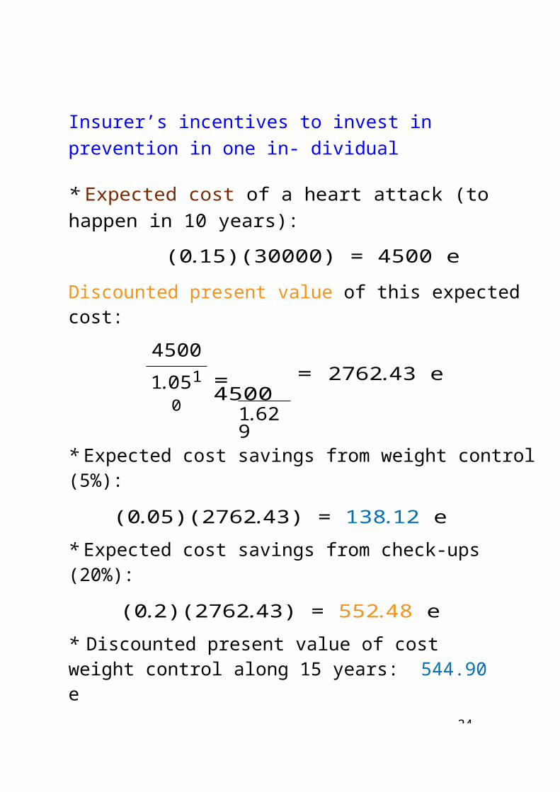
45

Illustration:

Evolution GDP n and GDP r Spain 1995-2003 (106

e).

Year GDPn price index GDPr1995 437.783 100 437.7831996 464.251 103.5 448.4571997 494.140 105.9 466.5131998 527.975 108.5 486.7851999 565.419 111.4 507.3462000 610.541 115.3 529.6912001 653.927 120.1 544.4962002 698.589 125.5 556.6512003 744.754 130.5 570.556

Source: INE.

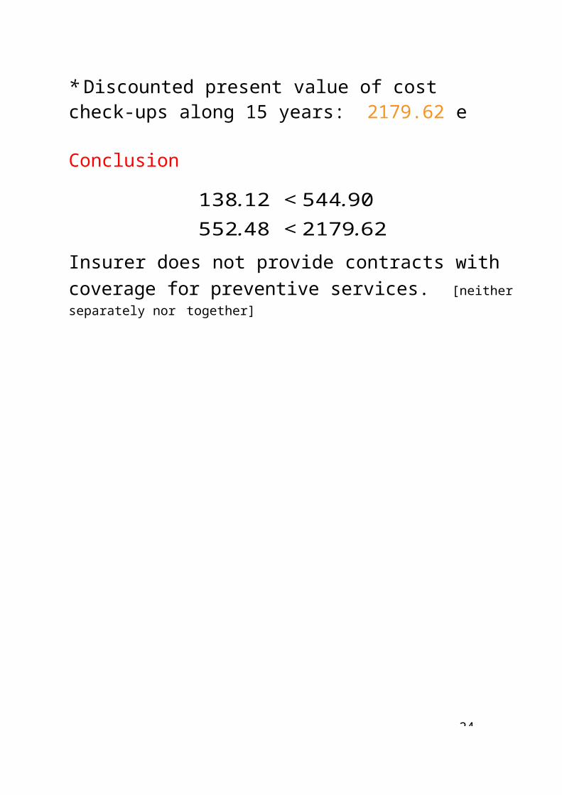
4

The working of the Economy

Model of aggregate demand and supply:

(1) understand incidence of the different forces on macro variables, and

(2) measure potential effectiveness of economic policies.

Aggregate demand is (the value of) the total quantity the different sectors of the economy are willing to spend in a particular period.

Graphically, market demand curve: relation between general price level of the economy and aggregate spending in goods and services in the economy.

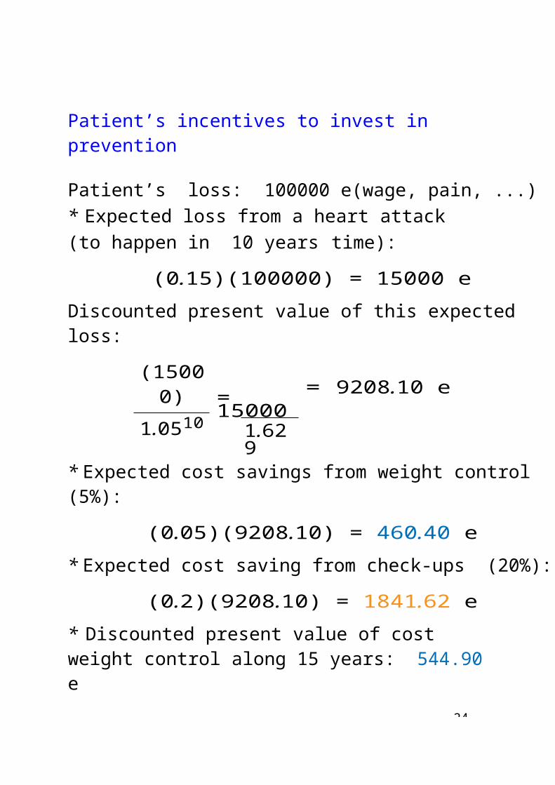
46-

Aggregate supply: (value of the) total quantity of goods and services firms in the country are willing to produce in a given period.

The market supply curve shows the production level firms are willing to supply at any given price level.

Macroeconomic equilibrium: characterization of the production level and of the price level.

Graphically: intersection point of aggregate demand and supply curves. Compatibility between consumers and producers behavior.

Equilibrium: two (potential) problems1. negative results: equilibrium price-production pair may not satisfy macro objectives (inflation, unemployment, investment level, ...)2. unstable results: even if the economy reaches optimal equilibrium may be perturbed by external shocks. oil crisis, bird flu, ...

=⇒ MACROECONOMIC POLICY

46-

Supply

Demand

Supply

Economicpolicy action

Supplyshock

Demandshock

DemandEconomic policy action

Aggregate supply and demand curves are shifted by changes in consumers and/or producers behavior (endogenous and/or exogenous shocks).

Options of the macroeconomic policy:

1. shift demand curve through fiscal and monetary policy;

2. shift supply curve through R&D policies;

3. do nothing if the causes of the perturbation are not identified.

P P

P* P*

Q* Q Q* Q

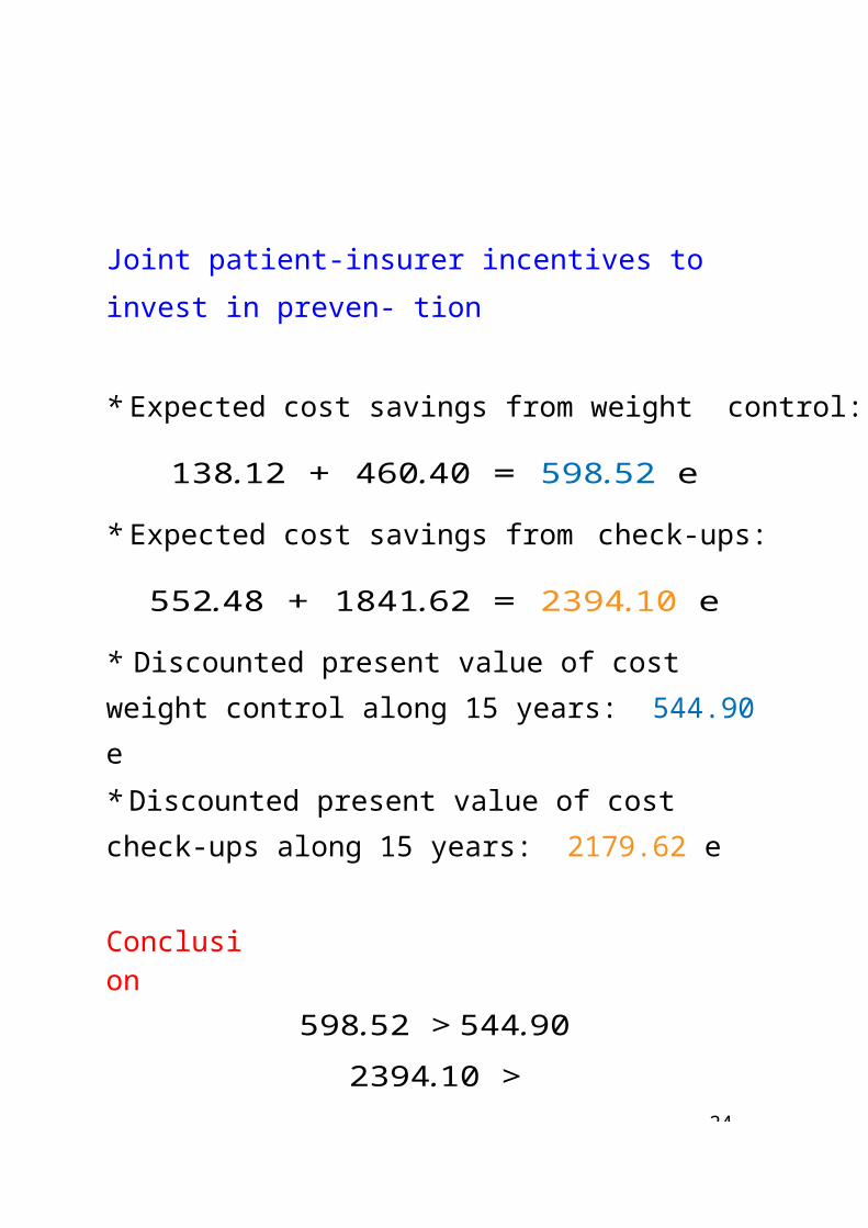
4

Unemployment.

Objective: maximize employment level.

Active population: set of people legally able to work= employed + unemployed.

Activity rate: (employed/active pop.)*100

Unemployment rate: (unemployed/employed)*100.

Labor market equilibrium: wage level inducing compatibility between labor supply and demand.

Full employment /= absence of unemployment −→frictional unemployment (3% − 5%).

Structural unemployment: lack of adjustment between labor demand and supply. (labor market rigidi- ties, professional qualifications, ...)

Frictional + structural unemployment = involuntary unemployment = unemployment rate.

47-

Measuring Unemployment.

“Encuesta de Poblacioń Activa” (Active population enquiry): estimated unemployment [harmonized across OECD countries].

Sampling on population −→ number of employed, unemployed, discouraged, by age, sex, education level, length of unemployment, etc.

Def.: unemployed individual not working the previous week, but ready to take a job along the following two weeks.

Def.: employed individual with a job (≥ 1 hour) in the previous week.

Active population = population employed + population unemployed.

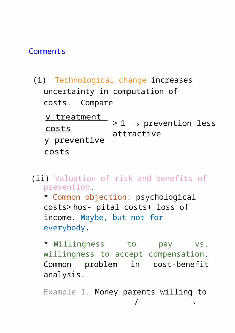
47-

alt

tinez-Gir Mar

X

avier

Qc

Health of

inciples Pr

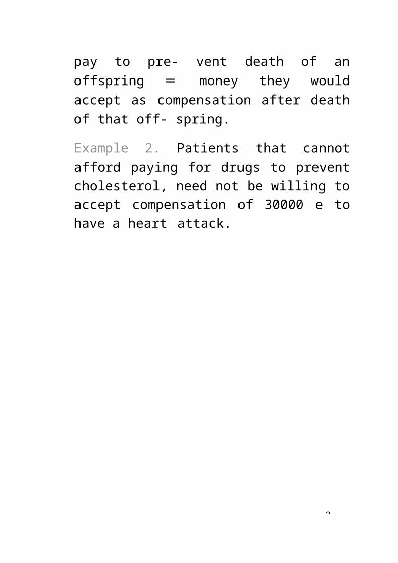
47

alt

tinez-Gir Mar

Xavier

Qc

Economics

Healthof

inciples Pr

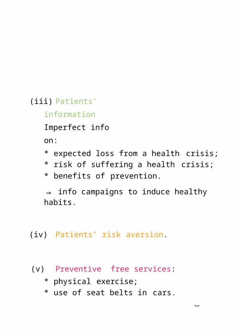
4

app app ora ora

Inflation.

Sustained and generalized increase of the general level of prices of goods and services in an economy.

How to define that price level? → Two alternative price indices (weighted average of prices):

1. GDP deflator,

2. CPI (Consumer price index).

* GDP deflator

GDP deflator = (nominal GDP)/(real GDP).

In our economy with oranges and apples,

(P 2006 ∗ Q2006) + (P 2006 ∗ Q2006)GDP deflator = app app ora ora .

(P 1996 ∗ Q2006) + (P 1996

∗ Q2006)

4

Comparison of a consumption bundle evaluated at today’s prices and at the base year prices.

48-

* Consumer Price Index.

CPI = nominal value of consumption bundle/real value of that consumption bundle.

consumption bundle: “Encuesta de Presupuestos Familiares del INE” → representative sample of consumption goods of families weighted by their importance.

CPI evolution: monthly, yearly, aggregated within the year, last 12 months.

Disaggregate CPI in sectorial price indices: non- energy goods and services, energy goods and services, non-manipulated food, ... → analyze their evolution. (See sample figures)

48-

alt

tinez-Gir Mar

Xavier

Qc

Economics

Healthof

inciples Pr

48

alt

tinez-Gir Mar

vier cXa

Economic

s Healthof

inciples Pr

CPI and price index of non elaborated produced goods and services excluding fats, tobacco and touristic packs.

Price index of non elaborated produced goods and services excluding fats and tobacco (BENE-X), and price index of services excluding touristic

packs (SERV-T).

48-

CPI vs. GDP deflator

1. GDP deflator measures the prices of all goods and services produced.CPI measures prices of goods and services in the representative consumption bundle.

2. GDP deflator considers only goods and services produced inside the country.

3. CPI is computed for a fixed consumption bundle; GDP deflator allows for variations of the bundle along time in accordance with the variation in the composition of the GDP.

4. CPI does not measure possibility of consumers to alter the composition of the bundle (neither substitution nor income effects.

Although CPI may differ from GDP, both convey the same info on the rhythm of price increase. See next figure.

48-

Mar

Xavier

Qc

Economics

Healthof

%

CPI

GDPdeflator

Year

Illustration:

Source: US Department of Commerce, Department of Labor.

48

Phillips curve

The Phillips curve.

Inverse relationship between inflation rate and unemployment rate. Controversial!!!

Reductions of unemployment rate against increases in inflation rate;

If prices moderate their increment, will yield an increase in unemployment.

unemployment

The Natural Unemployment Rate

In the long term the economy tends towards an unemployment rate independent of the implementation of fiscal and/or monetary policies (with only short run effects).

Infla

tion

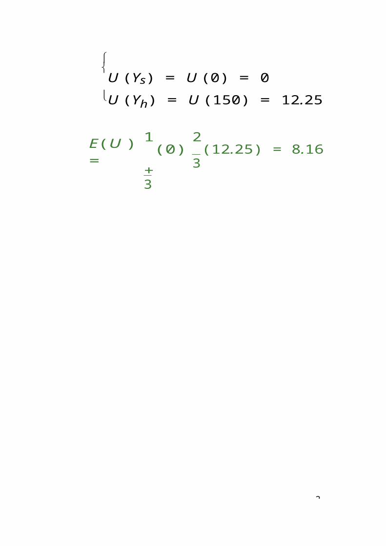
48-

Martin

Xavier

Unemployment rate

Illustration: US 1960-1995.

∗ 1960-1969: good fit (increasing inflation). Average inflation 2.5%, unemployment 4.8%

* 1970-1973: change in expectations (curve shifts). Average inflation and unemployment 5.2%

◦ 1974-1983: oil shock. Worse fit. Average inflation 8.2%, unemployment 7.5%

• 1984-1995: improve expectations. Average inflation 3.7%, unemployment 6.2%

Controversy: curve shifts vs. existence of the curve.

Infla

tion

rate

4

Macroeconomics of the health care market

Variables: 4 groups

* population health status- Life expectation at birth- Mortality rate- other: quality of life, morbidity, ...

* Life style and behavior- consumption of tobacco, alcohol and other drugs- other: education rate, ...

* Level of health services- health expenditure per capita- other: % hospital and pharma expenditure, ...

* Health promotion- % health care over GDP- other: number physicians, nurses, ...

49-

Lo

Lo

Relation between macro and health variables

* Economic growth

0 Positive effects on health:

- Life expectancy at birth: Spain 1960-97. in 8 years (70 to 78, both sexes)

- Child mortality rate: Spain 1975-1997.♦ neonatal + postneonatal: v 21/1000 to 6/1000♦ perinatal: v 19/1000 to 5/1000

0 Negative effects on health:

- Suicide and selfinjuries rate: Spain 1960-97. smooth since 1975

- tobacco consumption: Spain 1960-97. Lo 1000 ciggarettes/inhab/year. →

- Lung cancer mortality rate: 21/105 to 69/105

(males)

Source: Corugedo et al. (1999, p. 273-276)

Lo

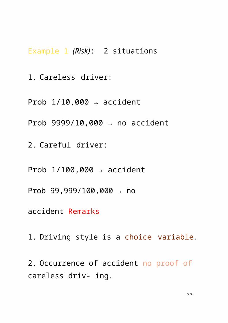
49-

* Economic development and health expenditure

Positive relation and more than proportional:

Lo Health expenditure > 1LoGDP

* Health expenditure and effects on health

Ambiguous effect. Decreasing returns of Health function →

Initial stages of a health system, big impact; Mature health systems modest impact.