Embed Size (px)
Citation preview

Biometrics 000, 1–6 DOI: 000
000 0000
Web Supplementary Materials for ‘Modeling Multiple Correlated Functional
Outcomes with Spatially Heterogeneous Shape Characteristics’
Kunlaya Soiaporn1,∗, David Ruppert1,∗∗, and Raymond J. Carroll2,∗∗∗
1School of Operations Research and Information Engineering, Cornell University, New York 14853, U.S.A.
2Department of Statistics, Texas A&M University, Texas, 77843, U.S.A.
*email: [email protected]
**email: [email protected]
***email: [email protected]
This paper has been submitted for consideration for publication in Biometrics

Modeling Multiple Correlated Functional Outcomes 1
1. Web Appendix A: Computation for EM Algorithm
1.1 The E-Step
Let E∗(·) denote the expectation given the observed data {Rip}. The goal of this step is to
compute E∗(Zip), E∗(ZipZ
Tip) and E∗(Zip, Zip′). Suppose Zi|Ri ∼ N(mi, Vi). That is,
f(Zi|Ri) ∝ exp{−(1/2)(Zi −mi)
TV −1i (Zi −mi)
}. (1)
Since f(Zi|Ri) ∝ f(Zi, Ri) and
f(Zi, Ri) ∝ exp
[−1
2
{∑p
1
σ2ϵp
(Rip −BΘpZip)T (Rip −BΘpZip) + ZT
i Σ−1Zi
}]
∝ exp
{−1
2
(∑p
1
σ2ϵp
ZTipΘ
TpB
TBΘpZip + ZTi Σ
−1Zi
)+∑p
1
σ2ϵp
RTipBΘpZip
}
= exp
{−1
2ZT
i (ETE + Σ−1)Zi +MiZi
}, (2)
where
Mi =
[1σ2ϵ1RT
i1BΘ11σ2ϵ2RT
i2BΘ2 · · · 1σ2ϵPRT
iPBΘP
]1×
∑p Kp
(3)
E =
1σϵ1
BΘ1 0
. . .
0 1σϵP
BΘP
mP×
∑p Kp
. (4)
Comparing the two expressions, we have that
Vi =(ETE + Σ−1
)−1= V ; (5)
mi = V TMTi . (6)
2 Biometrics, 000 0000
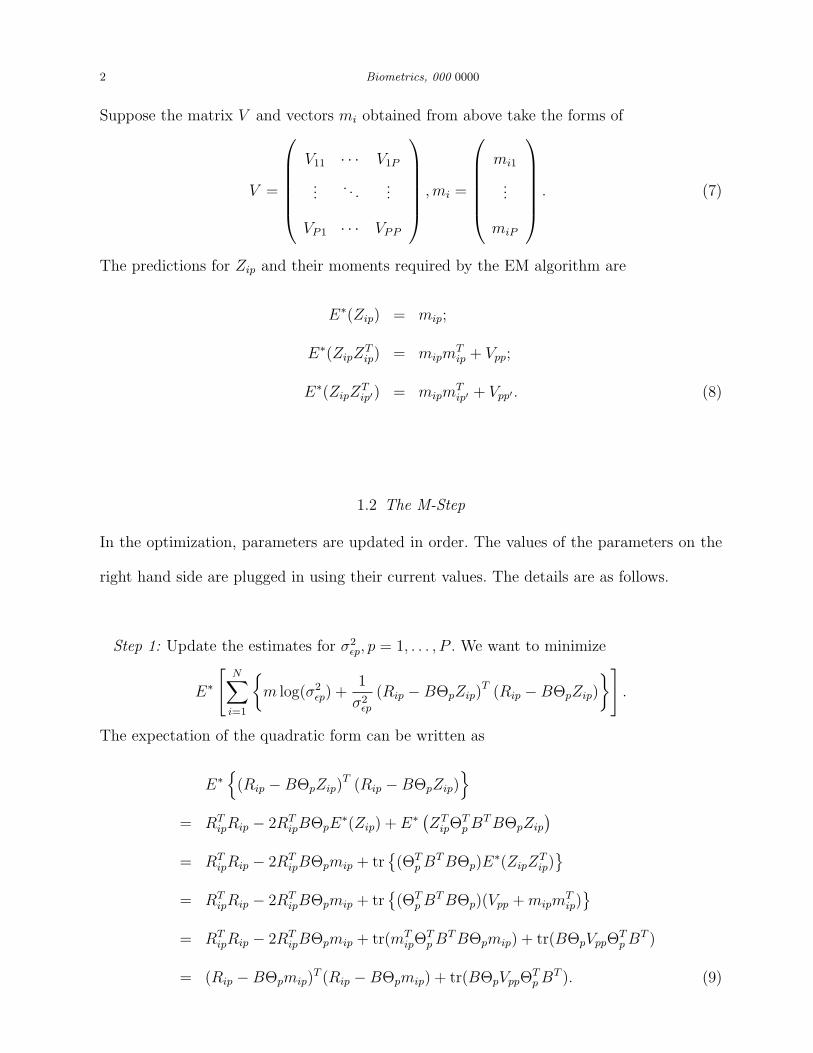
Suppose the matrix V and vectors mi obtained from above take the forms of
V =
V11 · · · V1P
.... . .
...
VP1 · · · VPP
,mi =
mi1
...
miP
. (7)
The predictions for Zip and their moments required by the EM algorithm are
E∗(Zip) = mip;
E∗(ZipZTip) = mipm
Tip + Vpp;
E∗(ZipZTip′) = mipm
Tip′ + Vpp′ . (8)
1.2 The M-Step
In the optimization, parameters are updated in order. The values of the parameters on the
right hand side are plugged in using their current values. The details are as follows.
Step 1: Update the estimates for σ2ϵp, p = 1, . . . , P . We want to minimize
E∗
[N∑i=1
{m log(σ2
ϵp) +1
σ2ϵp
(Rip −BΘpZip)T (Rip −BΘpZip)
}].
The expectation of the quadratic form can be written as
E∗{(Rip −BΘpZip)
T (Rip −BΘpZip)}
= RTipRip − 2RT
ipBΘpE∗(Zip) + E∗ (ZT
ipΘTpB
TBΘpZip
)= RT
ipRip − 2RTipBΘpmip + tr
{(ΘT
pBTBΘp)E
∗(ZipZTip)}
= RTipRip − 2RT
ipBΘpmip + tr{(ΘT
pBTBΘp)(Vpp +mipm
Tip)}
= RTipRip − 2RT
ipBΘpmip + tr(mTipΘ
TpB
TBΘpmip) + tr(BΘpVppΘTpB
T )
= (Rip −BΘpmip)T (Rip −BΘpmip) + tr(BΘpVppΘ
TpB
T ). (9)

Modeling Multiple Correlated Functional Outcomes 3
So, we want to minimize
Nm log(σ2ϵp) +
1
σ2ϵp
N∑i=1
{(Rip −BΘpmip)
T (Rip −BΘpmip) + tr(BΘpVppΘTpB
T )}. (10)
Hence, we update σ2ϵp by
σ2ϵp =
1
Nm
N∑i=1
{(Rip −BΘpmip)
T (Rip −BΘpmip) + tr(BΘpVppΘTpB
T )}, (11)
for each p = 1, . . . , P .
Step 2: Update Θp, by updating each column Θpk sequentially. For each k, we want to
minimize
N∑i=1
E∗
(∥Rip −
∑l =k
BΘplZipl −BΘpkZipk∥2)
+ σ2ϵpλpΘ
Tpk
∫b′′(t)b′′(t)TdtΘpk. (12)
Similar to the first step, the expression is minimized when
Θpk =
{N∑i=1
E∗(Z2ipk)B
TB + σ2ϵpλp
∫b′′(t)b′′(t)Tdt
}−1
×N∑i=1
BT
{RipE
∗(Zipk)−∑l =k
BΘplE∗(ZipkZipl)
}, (13)
where E∗(Z2ipk), E
∗(Zipk) and E∗(ZipkZipl) are the (k, k)−, k− and (k, l)− element ofmipmTip+
Vpp, mip and mipmTip′ + Vpp′ , respectively.
Step 3: Update Σ. We want to minimize
E∗
{N∑i=1
(log |Σ|+ ZT
i Σ−1Zi
)}=
N∑i=1
[log |Σ|+ tr
{Σ−1(V +mim
Ti )}]
. (14)
Since S =∑
i
(V +mim
Ti
)is positive-definite, there is a unique positive-definite matrix S1/2
such that S1/2S1/2 = S. Let W = S1/2Σ−1S1/2. Then we want to minimize
N log |Σ|+ tr(SΣ−1) = −N log |W |+N log |S|+ tr(W ). (15)
The positive-definite W can be diagonalized to get the diagonal elements τ1, . . . , τK , where

4 Biometrics, 000 0000
K =∑P
p=1Kp. What we finally want to minimize is −N∑K
k=1 log τk+∑K
k=1 τk. The solution
is τk = N for all k. That is, W = NIK which implies that Σ = S1/2W−1S1/2 = 1NS. Hence,
in this step, we update Σ by
Σ =1
NS =
1
N
∑i
(V +mimTi ). (16)
Step 4: Orthogonalization and update of the covariance matrix. Suppose the matrix Σ
obtained in step 3 takes the form
Σ =
Λ11 Λ12 · · · Λ1P
Λ21 Λ22 · · · Λ2P
......
. . ....
ΛP1 ΛP2 · · · ΛPP
. (17)
Let ΘpΛppΘTp = QpSpQ
Tp be the eigenvalue decomposition in which Qp has orthogonal
columns, and Sp is diagonal with diagonal elements in a decreasing order. We update Θp
by Qp and Dp by Sp. Since the updating in this step corresponds to the transformation
Zip ← QTp ΘpZip, we update Cpp′ by QT
p ΘpΛpp′ΘTp′Qp′ . The sign of each column of Θ is
changed as necessary so that the elements with the largest magnitude of each column are
positive.
2. Web Appendix B: Simulation Results
Figure S1 shows the estimates of mean, standard deviation and shape parameter functions
from 100 simulated datasets. The black lines are the true values, and the gray lines are the
estimates. The data were generated using a skew normal distribution as explained in the
main paper. Even though there seems to be high variation in the estimates when α ≈ 10,
the density of skew normal with α equal to 10 is not much different from when α is much
higher. This means that we can still obtain a good estimate for the distribution even though
the estimate for α in this range is not very accurate.

Modeling Multiple Correlated Functional Outcomes 5
[Figure 1 about here.]
Figure S2 shows the true and estimated correlations and cross correlations. The true
correlations within an outcome are shown in rows 1 and the true cross correlations are
shown in row 4. The estimated correlations within an outcome from 2 datasets are shown in
rows 2 and 3. The estimated cross correlations from the same 2 datasets are shown in rows
5 and 6.The estimated variances of each latent process are shown in Figure S3. The values
close to 1 indicate the closeness to our assumption that the latent processes have marginal
variance of 1.
[Figure 2 about here.]
[Figure 3 about here.]
Table S1 shows the square root of the integrated mean square error (IMSE), integrated
square bias (IBIAS) and integrated variance (IVAR) for the marginal parameter function
and covariance parameters, as defined in the main paper. The contour plots of the pointwise
square root of the mean square error for the covariance estimates are shown in Figure S4.
[Table 1 about here.]
[Figure 4 about here.]
3. Web Appendix C: Additional DTI Results
Figure S5 shows the estimates for the mean, variance and skewness for the three outcomes
for both groups. The black lines are the estimates for the MS group and the red lines are
the estimates for the healthy control group.
[Figure 5 about here.]
Figure S6 and Figure S7 display the estimated correlations within each outcome and the
estimated cross correlations between outcomes for the healthy and MS groups.

6 Biometrics, 000 0000
[Figure 6 about here.]
[Figure 7 about here.]

Modeling Multiple Correlated Functional Outcomes 7
0.0 0.2 0.4 0.6 0.8 1.0
4.0
4.5
5.0
5.5
6.0
Mean function 1
0.0 0.2 0.4 0.6 0.8 1.0
2.5
3.0
3.5
4.0
Std.dev. function 1
0.0 0.2 0.4 0.6 0.8 1.0
−2
−1
01
2
Shape param. function 1
0.0 0.2 0.4 0.6 0.8 1.0
1314
1516
17
Mean function 2
0.0 0.2 0.4 0.6 0.8 1.0
24
68
1012
Std.dev. function 2
0.0 0.2 0.4 0.6 0.8 1.0
−20
−10
010
20
Shape param. function 2
0.0 0.2 0.4 0.6 0.8 1.0
1520
2530
3540
Mean function 3
0.0 0.2 0.4 0.6 0.8 1.0
34
56
78
910
Std.dev. function 3
0.0 0.2 0.4 0.6 0.8 1.0
−10
−5
05
10
Shape param. function 3
Figure S1. The estimates from 100 datasets of mean (first column), standard deviation(second column) and shape parameter (third column) functions for the simulated data. Blacklines are true values.

8 Biometrics, 000 0000
0.0 0.2 0.4 0.6 0.8 1.0
0.0
0.4
0.8
Cov(R1(t1),R1(t2))
t1
t 2
−0.4
−0.4
0.4
0.4 0.8 0.8
0.0 0.2 0.4 0.6 0.8 1.0
0.0
0.4
0.8
Cov(R2(t1),R2(t2))
t1
t 2
−0.4
−0.2 0.
6
0.0 0.2 0.4 0.6 0.8 1.0
0.0
0.4
0.8
Cov(R3(t1),R3(t2))
t1
t 2
0.2
0.2
0.8
0.8
0.0 0.2 0.4 0.6 0.8 1.0
0.0
0.4
0.8
Estimated Cov(R1(t1),R1(t2))
t1
t 2
−0.4
−0.4
0
0
0.8
0.8 0.0 0.2 0.4 0.6 0.8 1.0
0.0
0.4
0.8
Estimated Cov(R2(t1),R2(t2))
t1
t 2
−0.4
−0.4
0.6
0.6 1
0.0 0.2 0.4 0.6 0.8 1.0
0.0
0.4
0.8
Estimated Cov(R3(t1),R3(t2))
t1
t 2
0
0.2
0.4 0.6 0.6 0.8
0.0 0.2 0.4 0.6 0.8 1.0
0.0
0.4
0.8
Estimated Cov(R1(t1),R1(t2))
t1
t 2
−0.4
−0.4
0.4
0.4 0.8 0.8
0.0 0.2 0.4 0.6 0.8 1.0
0.0
0.4
0.8
Estimated Cov(R2(t1),R2(t2))
t1
t 2
−0.4
−0.2 0.
6
0.8 1
0.0 0.2 0.4 0.6 0.8 1.0
0.0
0.4
0.8
Estimated Cov(R3(t1),R3(t2))
t1
t 2
0
0.2
0.4
0.4 0.6
0.8
0.0 0.2 0.4 0.6 0.8 1.0
0.0
0.4
0.8
Cov(R1(t1),R2(t2))
t1
t 2
−0.2 0 0.2
0.0 0.2 0.4 0.6 0.8 1.0
0.0
0.4
0.8
Cov(R1(t1),R3(t2))
t1
t 2
0 0 0.2
0.0 0.2 0.4 0.6 0.8 1.0
0.0
0.4
0.8
Cov(R2(t1),R3(t2))
t1t 2
−0.2
−0.2
0
0 0.2
0.4
0.0 0.2 0.4 0.6 0.8 1.0
0.0
0.4
0.8
Estimated Cov(R1(t1),R2(t2))
t1
t 2
−0.2 0 0.2
0.0 0.2 0.4 0.6 0.8 1.0
0.0
0.4
0.8
Estimated Cov(R1(t1),R3(t2))
t1
t 2 −0.2
0 0
0.2
0.2
0.4 0.0 0.2 0.4 0.6 0.8 1.0
0.0
0.4
0.8
Estimated Cov(R2(t1),R3(t2))
t1
t 2
−0.2
0 0.2 0.4
0.0 0.2 0.4 0.6 0.8 1.0
0.0
0.4
0.8
Estimated Cov(R1(t1),R2(t2))
t1
t 2
−0.2 0 0.2
0.0 0.2 0.4 0.6 0.8 1.0
0.0
0.4
0.8
Estimated Cov(R1(t1),R3(t2))
t1
t 2
−0.2
0 0 0.2
0.2
0.4 0.0 0.2 0.4 0.6 0.8 1.0
0.0
0.4
0.8
Estimated Cov(R2(t1),R3(t2))
t1
t 2
−0.2
−0.2
0
0 0.2
0.4
Figure S2. True and estimated covariances within each outcome and cross-covariancesbetween outcomes. The true covariances and cross covariances are shown in rows 1 and 4,respectively. The estimated covariances within each outcome from 2 datasets are shown inrows 2 and 3. Rows 5 and 6 are the estimated cross-covariances from the same datasets.Thus, rows 2 and 3 should be compared with row 1 and rows 5 and 6 with row 4.

Modeling Multiple Correlated Functional Outcomes 9
Estimated variance of Rp(t)
0.9
1.1
0.9
1.1
0.9
1.1
0 0.1 0.3 0.5 0.7 0.9 1
p=1 p=2 p=3
t
Figure S3. 100 estimates of the variance of the latent processes for the simulated data.Black, red and blue lines are the true values, which are 1.

10 Biometrics, 000 0000
0.0 0.2 0.4 0.6 0.8 1.0
0.0
0.2
0.4
0.6
0.8
1.0
MSEof Cov(R1(t1),R1(t2))
t1
t 2
0.01
0.01
0.02
0.0
2
0.0
3
0.0
3 0.0
4 0
.04
0.06
0.06
0.0 0.2 0.4 0.6 0.8 1.0
0.0
0.2
0.4
0.6
0.8
1.0
MSEof Cov(R2(t1),R2(t2))
t1
t 2
0.02
0.02
0.02
0.03 0.03 0
.04
0.0
4
0.05
0.0
5
0.07
0.0 0.2 0.4 0.6 0.8 1.0
0.0
0.2
0.4
0.6
0.8
1.0
MSEof Cov(R3(t1),R3(t2))
t1
t 2
0.01
0.01
0.0
2
0.0
2
0.0
3
0.0
3 0.0
4
0.05
0.0
6
0.06
0.07
0.07
0.0 0.2 0.4 0.6 0.8 1.0
0.0
0.2
0.4
0.6
0.8
1.0
MSEof Cov(R1(t1),R2(t2))
t1
t 2
0.06
0.06
0.07
0.0
7
0.0 0.2 0.4 0.6 0.8 1.0
0.0
0.2
0.4
0.6
0.8
1.0
MSEof Cov(R1(t1),R3(t2))
t1
t 2
0.06 0
.07
0.07
0.0 0.2 0.4 0.6 0.8 1.0
0.0
0.2
0.4
0.6
0.8
1.0
MSEof Cov(R2(t1),R3(t2))
t1
t 2
0.06 0.07
0.0
7
Figure S4. Pointwise square root of MSE for covariance within and between outcomes ofthe 100 estimates for the simulated data.

Modeling Multiple Correlated Functional Outcomes 11
0.0 0.2 0.4 0.6 0.8 1.0
0.45
0.60
Fractional anisotropy
Tract distanceM
ean
0.0 0.2 0.4 0.6 0.8 1.0
1.3
1.5
1.7
Parallel diffusivity
Tract distance
Mea
n
MScontrol
0.0 0.2 0.4 0.6 0.8 1.0
0.5
0.7
0.9
Perpendicular diffusivity
Tract distance
Mea
n
0.0 0.2 0.4 0.6 0.8 1.0
0.00
20.
008
Tract distance
Var
ianc
e
0.0 0.2 0.4 0.6 0.8 1.0
0.00
0.04
0.08
Tract distance
Var
ianc
e
0.0 0.2 0.4 0.6 0.8 1.0
0.00
0.03
Tract distance
Var
ianc
e
0.0 0.2 0.4 0.6 0.8 1.0
−0.
50.
5
Tract distance
Ske
wne
ss
0.0 0.2 0.4 0.6 0.8 1.0
0.0
1.0
Tract distance
Ske
wne
ss
0.0 0.2 0.4 0.6 0.8 1.0
−1.
00.
51.
5
Tract distance
Ske
wne
ss
Figure S5. Estimates of the mean, variance and skewness for the three outcomes for thehealthy control (red lines) and MS (black lines) groups. Gray dashed lines indicate zeroskewness.

12 Biometrics, 000 0000
0.0 0.4 0.8
0.0
0.4
0.8
t1
t 2
Fractional aniso.(control) 0 0.4
0.4
0.6
0.6
0.8
0.8
−1
−0.5
0
0.5
1
0.0 0.4 0.8
0.0
0.4
0.8
t1
t 2
Parallel diff.(control)
0
0
0.4
0.4
0.6
0.6 0.8
0.8
0.0 0.4 0.8
0.0
0.4
0.8
t1
t 2
0
0
0.4 0.4
0.4
0.4
0.6
0.6
Perpendicular diff.(control)
0.0 0.4 0.8
0.0
0.4
0.8
t1
t 2
0.4
0.4
0.6
0.6
0.6
0.8
0.8
Fractional aniso.(MS)
0.0 0.4 0.80.
00.
40.
8
t1
t 2 0
0.2
0.2 0.4
0.4
0.6
0.6 0.8
0.8
Parallel diff.(MS)
0.0 0.4 0.8
0.0
0.4
0.8
t1
t 2
0.4
0.4
0.6
0.6
0.8
0.8
Perpendicular diff.(MS)
Figure S6. Estimated correlations within each outcome for the control group (left panel)and the MS group (right panel).

Modeling Multiple Correlated Functional Outcomes 13
0.0 0.4 0.8
0.0
0.4
0.8
Fractional aniso.
Par
alle
l diff
.
0
0
0 0
.2
0.2 0.2
0.2
Control
−1
−0.5
0
0.5
1
0.0 0.4 0.8
0.0
0.4
0.8
Fractional aniso.
Per
pend
icul
ar d
iff.
−0.6
−0.6
−0.
4
−0.4
−0.2 0 0
0.0 0.4 0.8
0.0
0.4
0.8
Parallel diff.
Per
pend
icul
ar d
iff.
−0.2 0
0 0 0.2
0.4 0.6
0.0 0.4 0.8
0.0
0.4
0.8
Fractional aniso.
Par
alle
l diff
.
−0.2
−0.2
0
0
0
MS
0.0 0.4 0.80.
00.
40.
8
Fractional aniso.
Per
pend
icul
ar d
iff. −0.6
−0.6
−0.4
−0.4
−0.2
0.0 0.4 0.8
0.0
0.4
0.8
Parallel diff.
Per
pend
icul
ar d
iff.
0
0.2
0.2
0.4
0.6
Figure S7. Estimated cross-correlations between different outcomes for the control group(left panel) and the MS group (right panel).

14 Biometrics, 000 0000
Table S1Estimates of the square roots of IMSE, IBIAS and IVAR for the simulated data from 100 datasets
Parameter√IMSE× 102
√IBIAS× 102
√IVAR× 102
µ1(t) 23.66 2.51 23.52µ2(t) 36.87 1.90 36.83µ3(t) 36.66 3.94 35.84
σ1(t) 16.72 2.20 16.58σ2(t) 29.24 1.78 29.19σ2(t) 28.57 3.36 28.37
α1(t) 98.00 6.93 97.76α2(t) 210.7 72.42 197.9α2(t) 105.6 16.71 104.2
cov (R1(t), R1(t)) 4.25 0.43 4.23cov (R2(t), R2(t)) 4.58 0.57 4.55cov (R3(t), R3(t)) 4.52 0.73 4.46cov (R1(t), R2(t)) 6.30 0.64 6.27cov (R1(t), R3(t)) 6.49 0.98 6.42cov (R2(t), R3(t)) 6.36 0.66 6.32