Web-based Supplementary Materials for“Parametric Functional Principal ComponentAnalysis” by Peijun Sang, Liangliang Wang,

and Jiguo Cao

1

S1 Applications

S1.1 Analysis of Medfly Data

S1.2 Analysis of longitudinal CD4 Counts

0 1 2 3 4 5 6

010

2030

4050

6070

Year

CD

4 P

erce

ntag

e

Figure S1: The CD4 percentage trajectories of 283 homosexual men.

2

1 2 3 4 5

0.00

50.

010

0.01

50.

020

0.02

50.

030

0.03

5

p

J(p)

Figure S2: The weighted distance J(p) of the FPCs estimated using parametricFPCA and nonparametric FPCA when the degree of polynomials p varies for thelongitudinal CD4 counts.

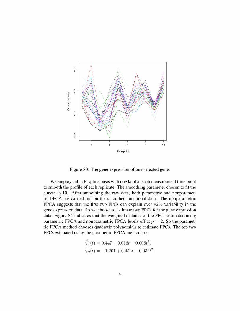
S1.3 Analysis of Gene Expression DataRangel et al. (2004) collected time course microarray data for T-cell activation toinvestigate a dynamic gene regulatory network. For the time course measurementof each gene, 10 unequally spaced observations are sampled; each gene has 34independent replicates. Here we analyze all 34 replicates of the time course mea-surements of one randomly selected gene. Figure S3 displays the gene expressionprofiles at each sampled point across the 34 replicates. Several fast oscillations arepresented in the profiles, which implies great within-curve variability. However,the profiles of the replicates appear similar, thus the between-curve variability ismuch smaller.

3

2 4 6 8 10

15.5

16.0

16.5

17.0

Time point

Gen

e ex

pres

sion

Figure S3: The gene expression of one selected gene.

We employ cubic B-spline basis with one knot at each measurement time pointto smooth the profile of each replicate. The smoothing parameter chosen to fit thecurves is 10. After smoothing the raw data, both parametric and nonparamet-ric FPCA are carried out on the smoothed functional data. The nonparametricFPCA suggests that the first two FPCs can explain over 92% variability in thegene expression data. So we choose to estimate two FPCs for the gene expressiondata. Figure S4 indicates that the weighted distance of the FPCs estimated usingparametric FPCA and nonparametric FPCA levels off at p = 2. So the paramet-ric FPCA method chooses quadratic polynomials to estimate FPCs. The top twoFPCs estimated using the parametric FPCA method are:

ψ̂1(t) = 0.447 + 0.016t− 0.006t2,

ψ̂2(t) = −1.201 + 0.452t− 0.032t2.

4

1 2 3 4 5

0.0

0.1

0.2

0.3

0.4

p

J(p)

Figure S4: The weighted distance J(p) of the FPCs estimated using parametricFPCA and nonparametric FPCA when the degree of polynomials p varies for thegene expression data.

Method FPC 1 FPC 2 TotalGene expression Parametric FPCA 80.49% 12.26% 92.75%

Nonparametric FPCA 80.55% 12.33% 92.88%Method FPC 1 FPC 2 FPC 3 Total

Hip angle Parametric FPCA 72.60% 11.53% 8.35% 92.48%Nonparametric FPCA 72.67% 12.29% 8.50% 93.46%

Method FPC 1 TotalGirl height Parametric FPCA 89.14% 89.14%

Nonparametric FPCA 89.30% 89.30%Method FPC 1 Total

Log-precipitation Parametric FPCA 86.66% 86.66%Nonparametric FPCA 87.38% 87.38%

Table S1: Comparison of variations explained by the leading FPCs estimated fromparametric FPCA and nonparametric FPCA for all four application cases.

A performance comparison of the first two FPCs obtained using the nonpara-

5

metric and parametric methods can be found in Table S1. The parametric esti-mates compare favorably with the nonparametric estimates in terms of capturingthe variability in the smoothed sample curves. What’s more, significant parallelsbetween the two sets of estimates of the first two FPCs are observable from FigureS5, which further justifies that parametric FPCA can rival nonparametric FPCA.

2 4 6 8 10

0.0

0.1

0.2

0.3

0.4

Time

FP

C 1

P−FPCANP−FPCA

2 4 6 8 10

−0.

6−

0.2

0.2

Time

FP

C 2

P−FPCANP−FPCA

Figure S5: The top two FPCs estimated using nonparametric FPCA and paramet-ric FPCA for gene expression data. P-FPCA stands for parametric FPCA; whileNP-FPCA stands for nonparametric FPCA.

Using the parametric FPCA method, around 80.5% of total variability in thegene expression data is accounted for by the first FPC. There is no change in thesign of it over the whole time interval; it can be regarded as “average” of all curvesin the sample. Unlike the first FPC being constantly positively valued, the signof the second FPC changes from negative to positive at time 3.5, which may beinterpreted as the change of gene expression after the time 3.5.

S1.4 Analysis of hip angle dataThe hip angle data consists of the angles formed by the hips of 39 children overeach child’s gait cycle (Ramsay and Silverman (2005)). This dataset is presented

6

in Figure S6. Since data exhibit some periodic characteristics, we employed 65Fourier basis functions of period 1 to smooth the profiles of each child. Thesmoothing parameter λ is set to 10−7 based on the GCV criterion with degrees offreedom multiplied by 1.2, as suggested by Gu (2013). Next both parametric andnonparametric FPCA methods are exploited to estimate FPCs for the smoothedfunctional data. The nonparametric FPCA method estimates the FPCs as linearcombinations of the 65 Fourier basis functions of period 1. It suggests that the firstthree FPCs can explain over 85% variability in the hip angle data. So we chooseto estimate three FPCs for the hip angle data. Figure S7 shows that the weighteddistance of the FPCs estimated using parametric FPCA and nonparametric FPCAlevels off at p = 4. So the parametric FPCA method chooses quartic polynomialsto estimate FPCs. The parametric FPCA estimates of the top three FPCs are givenby:

ψ̂1(t) = 1.140 + 2.489t− 17.938t2 + 29.109t3 − 13.519t4,

ψ̂2(t) = 0.385 + 11.131t− 41.242t2 + 30.104t3 + 0.790t4,

ψ̂3(t) = −0.071 + 15.080t− 108.701t2 + 196.009t3 − 102.037t4.

7

0.0 0.2 0.4 0.6 0.8 1.0

020

4060

Time

Hip

Ang

le

Figure S6: The trajectories of hip angles of 39 children over their gait cycles.

8

2 3 4 5 6

0.26

0.27

0.28

0.29

p

J(p)

Figure S7: The weighted distance J(p) of the FPCs estimated using parametricFPCA and nonparametric FPCA when the degree of polynomials p varies for thehip angle data.

From Table S1 we see that the proportion of variability explained by the firstthree FPCs is again highly comparable between the parametric and nonparametricmethods. Figure S8 illustrates that the shapes of the FPCs are similar, especiallythose of the first two FPCs. Compared with parametric FPCA estimate, the thirdFPC estimated using the nonparametric FPCA is considerably more wiggly, espe-cially near the lower and upper tails. This effect may be due to sparse samplings(edge effect). This fact is not surprising since the more flexible basis functionsused in nonparametric FPCA may introduce greater roughness.

9

0.0 0.2 0.4 0.6 0.8 1.0

0.7

0.8

0.9

1.0

1.1

1.2

time

FP

C 1

P−FPCANP−FPCA

0.0 0.2 0.4 0.6 0.8 1.0−

1.5

−0.

50.

00.

51.

0

time

FP

C 2

P−FPCANP−FPCA

0.0 0.2 0.4 0.6 0.8 1.0

−1.

00.

00.

51.

01.

5

time

FP

C 3

P−FPCANP−FPCA

Figure S8: The top three FPCs estimated using nonparametric FPCA and para-metric FPCA for hip angle data. P-FPCA stands for parametric FPCA; whileNP-FPCA stands for nonparametric FPCA.

The estimate of the first FPC using parametric FPCA demonstrates incompara-ble in revealing the internal structure, explaining around 72.6% of total variabilityin the hip angle data; while the latter two explain respectively 11.5% and 8.4%of total variability in the hip angle data. The first FPC is positive in the wholetime interval without any sign change; in contrast both the second and third FPCschange sign twice. Therefore, the first FPC can be interpreted as a weighted aver-age of all values of each curve in the whole time interval; the second FPC, positivein [0, 0.42] and negative in [0.42, 0.94], may be interpreted as the change of hipangle after the time 0.42 when neglecting the fact that it is positive in [0.94, 1].This interpretation is acceptable since the interval [0.94, 1] is very short comparedwith the two longer intervals and thus makes little difference when taking this in-terval into consideration. Being positive in [0.20, 0.70] and negative elsewhere,the third FPC can be interpreted as the difference in hip angles during [0.20, 0.70]and other time.

S1.5 Analysis of girl height dataIn Berkeley Growth Study (Tuddenham and Snyder (1954)), the heights of 54 girlswere measured at a set of 31 different ages. Figure S9 describes how the heights ofthe 54 girls change from childhood to adolescence. We employ 33 cubic B-spline

10

basis functions with one knot at each measurement age to smooth the trajectory ofheights of each girl. The smoothing parameter λ is set to 0.1. Next we conductedboth nonparametric and parametric FPCA methods on the smoothed functionaldata. The nonparametric FPCA suggests that the first FPC can explain over 85%of the total variability in the girl height data. So we choose to estimate one FPCfor the girl height data. Figure S10 shows that the weighted distance of the FPCestimated using parametric FPCA and nonparametric FPCA levels off at p = 3.So the parametric FPCA method chooses cubic polynomials to estimate the FPC.The parametric FPCA estimate of the first FPC is given by:

ψ̂1(t) = 0.083 + 0.014t+ 1.8× 10−3t2 − 1.2× 10−4t3.

5 10 15

8010

012

014

016

018

0

Age

Hei

ght

Figure S9: The trajectories of heights of 54 girls from age 1 to 18.

11

1 2 3 4 5

0.1

0.2

0.3

0.4

0.5

p

J(p)

Figure S10: The weighted distance J(p) of the FPCs estimated using parametricFPCA and nonparametric FPCA when the degree of polynomials p varies for thegirl height data.

As indicated by Table S1, the performances of nonparametric FPCA and para-metric FPCA are quite similar with regard to the proportions of total variationexplained by the first FPC obtained using these two FPCA methods. Figure S11further illustrates the comparison of the first FPC.

12

5 10 15

0.10

0.15

0.20

0.25

0.30

age

FP

C 1

P−FpCANP−FPCA

Figure S11: The first FPC estimated using both nonparametric FPCA and para-metric FPCA for the girl height data. P-FPCA stands for parametric FPCA; whileNP-FPCA stands for nonparametric FPCA.

The parametric FPCA estimate of the first FPC is positive over the whole timeinterval and plays an indispensable role in revealing the internal structure of thecurves in the sample; it explains the bulk (89.1%) of total variability in the curvesof girl heights in the sample. We can interpret the first FPC as a weighted averageof all values of each curve in the whole time interval.

13

S1.6 Analysis of log-precipitation across CanadaThe next dataset of interest consists of daily precipitation collected by 35 Cana-dian weather stations (Ramsay and Silverman (2005)). Figure S12 demonstrateshow the daily precipitation changes over the course of one year. Since the precip-itation exhibits some periodic variations, we smooth the precipitation data using365 Fourier basis functions of period 365. The smoothing parameter λ is set to106, which minimizes the GCV measure with degrees of freedom multiplied by1.2, as suggested by Gu (2013). Then both parametric and nonparametric FPCAare performed on the smoothed daily log-precipitation data to estimate FPCs. Thenonparametric FPCA suggests that the first FPC can explain over 85% of the totalvariability in the precipitation data. So we choose to estimate one FPC for theprecipitation data. Figure S13 shows that the weighted distance of the FPC esti-mated using parametric FPCA and nonparametric FPCA levels off at p = 2. Sothe parametric FPCA method chooses quadratic polynomials to estimate the FPC.The first FPC estimated using parametric FPCA is:

ψ̂1(t) = 1.0× 10−3 + 6.7× 10−4t− 1.7× 10−6t2.

14

0 100 200 300

−1.

0−

0.5

0.0

0.5

1.0

Day

log 1

0(P

reci

pita

tion)

Figure S12: The trajectories of the daily (log) precipitation across one year for 35Canadian weather stations.

15

1 2 3 4 5

12

34

5

p

J(p)

Figure S13: The weighted distance J(p) of the FPCs estimated using parametricFPCA and nonparametric FPCA when the degree of polynomials p varies for thelog-precipitation data.

Table S1 shows that the proportions of variability explained by the first FPCare very similar, indicating that replacing the flexible nonparametric functionswith the simpler parametric functions will not cause a great loss in performance.In Figure S14 we see that the first FPCs using these two methods are highly anal-ogous.

16

0 100 200 300

0.00

0.01

0.02

0.03

0.04

0.05

0.06

0.07

Day

FP

C 1

P−FPCANP−FPCA

Figure S14: The first FPC estimated using nonparametric FPCA and parametricFPCA for log-precipitation data. P-FPCA stands for parametric FPCA; while NP-FPCA stands for nonparametric FPCA.

As demonstrated in previous examples, the bulk (86.7%) of variance of thecurves in the sample is accounted for by the first FPC estimated using parametricFPCA. Furthermore, the first FPC is positively valued over the whole time intervaland summarizes the average of all profiles in the sample.

17

S1.7 Analysis of Diffusion Tensor Imagining (DTI) data

0 20 40 60 80

0.4

0.5

0.6

0.7

0.8

Tract distance

Figure S15: Profiles of corpus callosum (cca) across 42 healthy controls.

18

2 3 4 5 6

1.0

1.5

2.0

2.5

3.0

p

J(p)

Figure S16: The weighted distance J(p) of the FPCs estimated using parametricFPCA and nonparametric FPCA when the degree of polynomials p varies for theDTI data.

0 20 40 60 80

0.07

0.09

0.11

0.13

Tract distance

FP

C 1

P−FPCANP−FPCA

0 20 40 60 80

−0.

2−

0.1

0.0

0.1

0.2

Tract distance

FP

C 2

P−FPCANP−FPCA

0 20 40 60 80

−0.

10.

00.

10.

20.

3

Tract distance

FP

C 3

P−FPCANP−FPCA

Figure S17: The top three FPCs estimated using nonparametric FPCA and para-metric FPCA for the DTI data. NP-FPCA stands for nonparametric FPCA; whileP-FPCA stands for parametric FPCA.

19

S2 Simulation Study

0 5 10 15 20 25

−40

−20

020

4060

80

t

X(t

)

Figure S18: The trajectories of 21 true curves and 9 outlier curves randomly se-lected from one simulation replicate. The solid (—–) and dashed (− − −) linesrepresent the true curves and outlier curves, respectively.

20

0 5 10 15 20 25

−0.

006

−0.

002

0.00

2

Time

Bia

s

0 5 10 15 20 25

−0.

020.

00

Time

Bia

s

0 5 10 15 20 25

−0.

020.

020.

06

Time

Bia

s

0 5 10 15 20 25

0.01

0.03

0.05

Time

Sta

ndar

d E

rror

0 5 10 15 20 25

0.01

60.

020

0.02

4

Time

Sta

ndar

d E

rror

0 5 10 15 20 25

0.01

00.

020

Time

Sta

ndar

d E

rror

0 5 10 15 20 25

0.01

0.03

0.05

Time

RM

SE

0 5 10 15 20 25

0.01

50.

025

0.03

5

Time

RM

SE

0 5 10 15 20 25

0.01

0.03

0.05

Time

RM

SE

Figure S19: The estimated bias, standard error and RMSE of the top three FPCsestimated from parametric FPCA and nonparametric FPCA when there is no out-lier curve. In each panel, the solid (—–) and dashed (− − −) lines representthe FPC estimated from parametric FPCA and nonparametric FPCA, respectively.The first, second and third columns correspond to the first, second and third FPCs,respectively.

21

0 5 10 15 20 25

−0.

020.

020.

06

Time

Bia

s

0 5 10 15 20 25

−0.

050.

000.

05

Time

Bia

s

0 5 10 15 20 25

−0.

8−

0.4

0.0

Time

Bia

s

0 5 10 15 20 25

0.00

50.

015

Time

Sta

ndar

d E

rror

0 5 10 15 20 25

0.05

0.10

0.15

Time

Sta

ndar

d E

rror

0 5 10 15 20 25

0.05

0.10

0.15

Time

Sta

ndar

d E

rror

0 5 10 15 20 25

0.01

0.03

0.05

Time

RM

SE

0 5 10 15 20 25

0.05

0.10

0.15

Time

RM

SE

0 5 10 15 20 25

0.2

0.4

0.6

0.8

Time

RM

SE

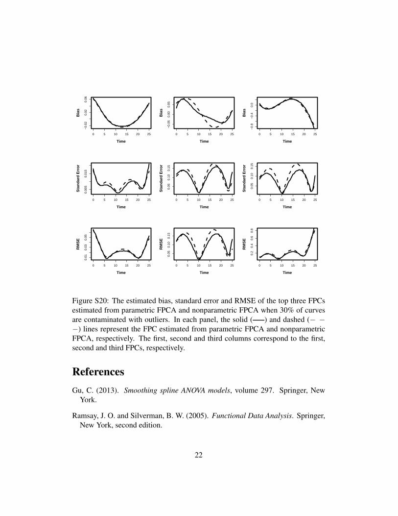
Figure S20: The estimated bias, standard error and RMSE of the top three FPCsestimated from parametric FPCA and nonparametric FPCA when 30% of curvesare contaminated with outliers. In each panel, the solid (—–) and dashed (− −−) lines represent the FPC estimated from parametric FPCA and nonparametricFPCA, respectively. The first, second and third columns correspond to the first,second and third FPCs, respectively.

ReferencesGu, C. (2013). Smoothing spline ANOVA models, volume 297. Springer, New

York.

Ramsay, J. O. and Silverman, B. W. (2005). Functional Data Analysis. Springer,New York, second edition.

22

Rangel, C., Angus, J., Ghahramani, Z., Lioumi, M., Sotheran, E., Gaiba, A., Wild,D. L., and Falciani, F. (2004). Modeling T-cell activation using gene expressionprofiling and state-space models. Bioinformatics, 20(9), 1361–1372.

Tuddenham, R. D. and Snyder, M. M. (1954). Physical growth of Californiaboys and girls from birth to eighteen years. Publications in child development.University of California, Berkeley, 1(2), 183–364.

23