Web-based analysis of (epi-) genome data using EpiGRAPH and Galaxy Christoph Bock1, 4, Greg Von Kuster2, Konstantin Halachev1, James Taylor3, Anton Nekrutenko2 and Thomas Lengauer1

1Max-Planck-Institut für Informatik, Saarbrücken, Germany 2Center for Comparative Genomics and Bioinformatics, Huck Institutes for Life Sciences, Penn State University, University Park, Pennsylvania 16802, USA 3Departments of Biology and Mathematics & Computer Science, Emory University, Atlanta, Georgia 30322, USA 4Corresponding author, e-mail address: cbock@mpi-inf.mpg.de

Keywords: Bioinformatics, genome analysis, statistics, machine learning, computational epigenetics, single nuc-leotide polymorphisms (SNPs), evolutionary constraint

Abstract Modern life sciences are becoming increasingly data intensive, posing a significant challenge for most researchers and shifting the bottleneck of scientific discovery from data generation to data analysis. As a result, progress in genome research is increasingly impeded by bioinformatic hurdles. A new genera-tion of powerful and easy-to-use genome analysis tools has been developed to address this issue, enabl-ing biologists to perform complex bioinformatic analyses online – without having to learn a program-ming language or downloading and manually processing large datasets. In this tutorial paper, we de-scribe the use of EpiGRAPH (http://epigraph.mpi-inf.mpg.de/) and Galaxy (http://galaxyproject.org/) for genome and epigenome analysis, and we illustrate how these two web services work together to identify epigenetic modifications that are characteristic of highly polymorphic (SNP-rich) promoters. This paper is supplemented by video tutorials (available online), which provide a step-by-step guide through each example analysis.

Introduction Vertebrate gene expression is regulated at several levels of control, which are tightly interlinked with each other (Bernstein, et al., 2007; Chen and Rajewsky, 2007). The key mechanism of DNA-based “genetic regulation” is transcription factor binding to sequence-specific recognition motifs, which are commonly located in promoter and enhancer regions (Zhang, 2005). In contrast, chromatin-based “epi-genetic regulation” comprises gene-regulatory mechanisms that are not directly controlled by the DNA sequence, such as chromatin condensation across an entire gene cluster (Frigola, et al., 2006). Variation in genetic and epigenetic gene regulation plays a major role in common diseases (Feinberg, 2007) and contributes to inter-individual differences in gene expression observed among healthy individuals (Bock, et al., 2008; Eckhardt, et al., 2006; Williams, et al., 2007). With the recent development of high-throughput protocols such as ChIP-on-chip and ChIP-seq (Schones and Zhao, 2008), it is now possible

to analyze genome-epigenome interactions and their impact on gene expression at a truly genomic scale.

However, such genome-wide analyses pose significant bioinformatic challenges. The goal of this paper is to illustrate the use of a new generation of web toolkits that enable biologists to perform com-plex (epi-) genome analyses online, without having to learn a programming language or to download large datasets onto a local computers. Specific focus will be put on a specialized tool for statistical analysis and prediction of (epi-) genome data, EpiGRAPH, and on a general-purpose platform for ma-nipulating large sets of genomic regions, Galaxy. The EpiGRAPH web service (Bock et al., submitted) provides a standardized workflow for identifying characteristic DNA attributes that are enriched in a given set of genomic regions, and for predicting similar regions across mammalian genomes. It is par-ticularly useful for explorative analysis and bioinformatic prediction, as is evident from applications to DNA methylation data (Bock, et al., 2006; Bock, et al., 2008), DNA melting profiles (Liu, et al., 2007), CpG island annotation (Bock, et al., 2007) and SNP function inference (Moser, et al., 2008). Compared to EpiGRAPH’s focus on a specific task, the Galaxy web service (Blankenberg, et al., 2007; Giardine, et al., 2005) is a general-purpose tool for processing any set of genomic regions. It provides simple and straightforward methods to join, merge, and intersect genomic regions, to map between formats, ge-nome assemblies and species, and to perform basic statistical analyses. In addition, it provides a user interface for more specialized toolkits such as HyPhy (Pond, et al., 2005), EMBOSS (Rice, et al., 2000) and EpiGRAPH. Here, we will illustrate the synergistic potential of EpiGRAPH and Galaxy for analyz-ing genome and epigenome datasets.

The remainder of the paper is structured as follows. First, the Materials section highlights the tech-nical prerequisites for using EpiGRAPH and Galaxy; second, we give an overview of available soft-ware tools that facilitate the analysis of epigenome datasets; third, we introduce EpiGRAPH by a sim-ple case study on DNA methylation analysis and prediction; fourth, we outline the use of Galaxy for performing calculations on sets of genomic regions; fifth, we describe an advanced case study that uses both EpiGRAPH and Galaxy in order to identify genomic and epigenomic characteristics that distin-guish highly polymorphic promoter regions from their non-polymorphic counterparts. Finally, in the Notes section we briefly comment on practical issues and highlight potential pitfalls of the methods that are outlined in this paper.

Materials The user must have access to a computer with Internet access, which could for example be a PC run-ning Microsoft Windows, an Apple computer running MacOS, or a UNIX workstation. Galaxy and Ep-iGRAPH are web toolkits and operated via a web browser, therefore it is important to have a sufficient-ly up-to-date web browser installed. Both toolkits have been tested with current versions of Mozilla Firefox (http://www.firefox.com/), Microsoft Internet Explorer (http://www.microsoft.com/ie/), Apple Safari (http://www.apple.com/de/safari/), KDE Konqueror (http://www.konqueror.org/) and Opera (http://www.opera.com/). Furthermore, the user should make sure that JavaScript and web browser cookies are enabled, since EpiGRAPH cannot be used without JavaScript, while Galaxy’s user-friendliness will be reduced when JavaScript is switched off).

Beyond the essential web browser, it is recommended to install an advanced text editor, e.g. EMACS (http://www.gnu.org/software/emacs/) or Programmer’s Notepad (http://www.pnotepad.org/), which can handle large files effectively and which simplifies any data formatting tasks that may be re-quired for a given dataset. Similarly, it is often helpful to copy and paste datasets into a spreadsheet

software such as Microsoft Excel (http://office.microsoft.com/en-us/excel/) or OpenOffice.org Calc (http://www.openoffice.org/product/calc.html), which facilitates adding, removing or rearranging col-umns in table-style datasets. For advanced users who want to perform data preparation steps or follow-up analyses in a simple programming environment, it is also useful to install the R statistics software (http://www.r-project.org/).

Finally, to be able to view the tutorial videos that accompany this paper, the Macromedia Flash Player and Apple QuickTime browser plug-ins are required, which can be freely downloaded from http://www.adobe.com/products/flashplayer/ and http://www.apple.com/quicktime/download/, respec-tively.

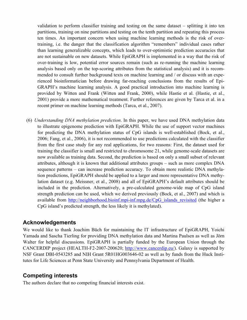
Methods A workflow for epigenome data analysis using web-based tools The analysis of epigenome datasets is often performed in four subsequent steps, as outlined in Figure 1. First, depending on the experimental method used to acquire the raw data, it is usually necessary to per-form specific data normalization and quality control steps, before a reliable set of enriched genomic regions can be derived. Second, visual inspection of the processed dataset provides a starting point for data analysis and often gives rise to biological hypotheses that can subsequently be tested with more quantitative methods. Third, extensive data processing is often necessary in order to identify and ex-tract a set of genomic regions that are relevant for a specific hypothesis. Fourth, statistical methods en-able researchers to rigorously test the validity of a given hypothesis, and exploratory data mining can be used to identify as yet unknown associations of the input dataset with other genomic and epigenomic attributes. The data analysis step often gives rise to new hypotheses that can form the starting point for further experiments and the next iteration of the analytical circle.

The third and fourth steps of this analysis workflow are addressed by Galaxy and EpiGRAPH, re-spectively, and are discussed in more detail in subsequent sections of this paper. In the current section, we briefly highlight key software toolkits that contribute to the first two steps.

Experimental methods for epigenome mapping – including ChIP-on-chip (van Steensel, 2005), ChIP-seq (Schones and Zhao, 2008) and DNA methylation analysis by bisulfite sequencing (Bernstein, et al., 2007) – require a significant amount of data preprocessing and quality control (step 1 in Figure 1), which is addressed by specific software toolkits (reviewed in Bock and Lengauer, 2008). For ChIP-on-chip, data preprocessing starts with microarray data normalization, which is often performed with either the Bioconductor package (Gentleman, et al., 2004) inside the R statistics software (http://www.r-project.org/) or a vendor-supplied tool. For ChIP-seq, the equivalent preprocessing step involves tag mapping to the genome assembly, which can be achieved using specialized BLAST-like tools such as Maq (http://maq.sourceforge.net/), ELAND (http://www.illumina.com/) or SXOligo-search (http://www.synamatix.com/). For both ChIP-on-chip and ChIP-seq, data preprocessing results in genome-scale profiles of over-representation scores, which can be visualized as quantitative tracks inside genome browsers. However, because such profiles often carry significant levels of biological and technical noise, it is in most cases advisable to perform peak-detection on these profiles, i.e. to identify sets of genomic regions that are enriched with high confidence (Liu, 2007). A recent ben-chmarking study of several peak-detection methods suggests that vendor-supplied tools perform suffi-ciently well (Johnson, et al., 2008). Further tools that – in our opinion – provide a good balance be-tween accuracy and user-friendliness are the web-based Splitter toolkit (http://zlab.bu.edu/splitter/) for NimbleGen and Agilent microarrays as well as the stand-alone MAT software (Johnson, et al., 2006)

for Affymetrix microarrays. For DNA methylation analysis, two experimental strategies are widely used. Antibody-based methods such as MeDIP-chip and MeDIP-seq give rise to similar bioinformatic issues as ChIP-on-chip or ChIP-seq, which can be addressed with the same toolkits. In contrast, DNA methylation analysis by bisulfite sequencing requires dedicated software. The QUMA web service (Kumaki, et al., 2008) provides a quick web-based solution for the analysis of clonal bisulfite sequenc-ing data. In contrast, the BiQ Analyzer software (Bock, et al., 2005) incorporates more extensive fea-tures for quality control and experiment documentation, but requires the user to download and install a small software tool.

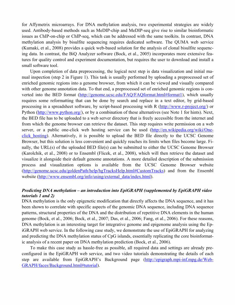
Upon completion of data preprocessing, the logical next step is data visualization and initial ma-nual inspection (step 2 in Figure 1). This task is usually performed by uploading a preprocessed set of enriched genomic regions into a genome browser, from which it can be viewed and visually compared with other genome annotation data. To that end, a preprocessed set of enriched genomic regions is con-verted into the BED format (http://genome.ucsc.edu/FAQ/FAQformat.html#format1), which usually requires some reformatting that can be done by search and replace in a text editor, by grid-based processing in a spreadsheet software, by script-based processing with R (http://www.r-project.org/) or Python (http://www.python.org/), or by a combination of these alternatives (see Note 1 for hints). Next, the BED file has to be uploaded to a web server directory that is freely accessible from the internet and from which the genome browser can retrieve the dataset. This step requires write permission on a web server, or a public one-click web hosting service can be used (http://en.wikipedia.org/wiki/One-click_hosting). Alternatively, it is possible to upload the BED file directly to the UCSC Genome Browser, but this solution is less convenient and quickly reaches its limits when files become large. Fi-nally, the URL(s) of the uploaded BED file(s) can be submitted to either the UCSC Genome Browser (Karolchik, et al., 2008) or to Ensembl (Flicek, et al., 2008), which will then retrieve the dataset and visualize it alongside their default genome annotations. A more detailed description of the submission process and visualization options is available from the UCSC Genome Browser website (http://genome.ucsc.edu/goldenPath/help/hgTracksHelp.html#CustomTracks) and from the Ensembl website (http://www.ensembl.org/info/using/external_data/index.html).

Predicting DNA methylation – an introduction into EpiGRAPH (supplemented by EpiGRAPH video tutorials 1 and 2) DNA methylation is the only epigenetic modification that directly affects the DNA sequence, and it has been shown to correlate with specific aspects of the genomic DNA sequence, including DNA sequence patterns, structural properties of the DNA and the distribution of repetitive DNA elements in the human genome (Bock, et al., 2006; Bock, et al., 2007; Das, et al., 2006; Fang, et al., 2006). For these reasons, DNA methylation is an interesting target for integrative genome and epigenome analysis using the Ep-iGRAPH web service. In the following case study, we demonstrate the use of EpiGRAPH for analyzing and predicting the DNA methylation status of CpG islands, essentially replicating the core bioinformat-ic analysis of a recent paper on DNA methylation prediction (Bock, et al., 2006).

To make this case study as hassle-free as possible, all required data and settings are already pre-configured in the EpiGRAPH web service, and two video tutorials demonstrating the details of each step are available from EpiGRAPH’s Background page (http://epigraph.mpi-inf.mpg.de/Web-GRAPH/faces/Background.html#tutorial).

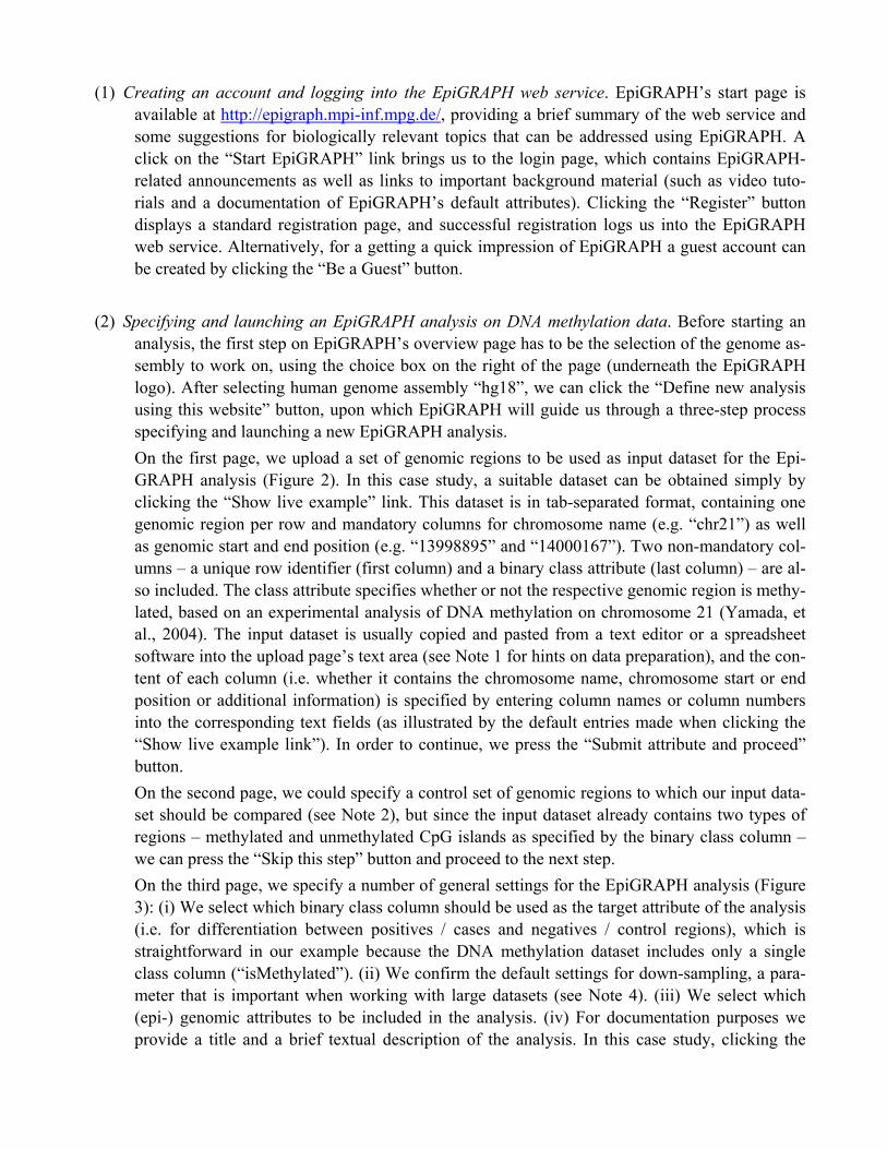
(1) Creating an account and logging into the EpiGRAPH web service. EpiGRAPH’s start page is available at http://epigraph.mpi-inf.mpg.de/, providing a brief summary of the web service and some suggestions for biologically relevant topics that can be addressed using EpiGRAPH. A click on the “Start EpiGRAPH” link brings us to the login page, which contains EpiGRAPH-related announcements as well as links to important background material (such as video tuto-rials and a documentation of EpiGRAPH’s default attributes). Clicking the “Register” button displays a standard registration page, and successful registration logs us into the EpiGRAPH web service. Alternatively, for a getting a quick impression of EpiGRAPH a guest account can be created by clicking the “Be a Guest” button.

(2) Specifying and launching an EpiGRAPH analysis on DNA methylation data. Before starting an

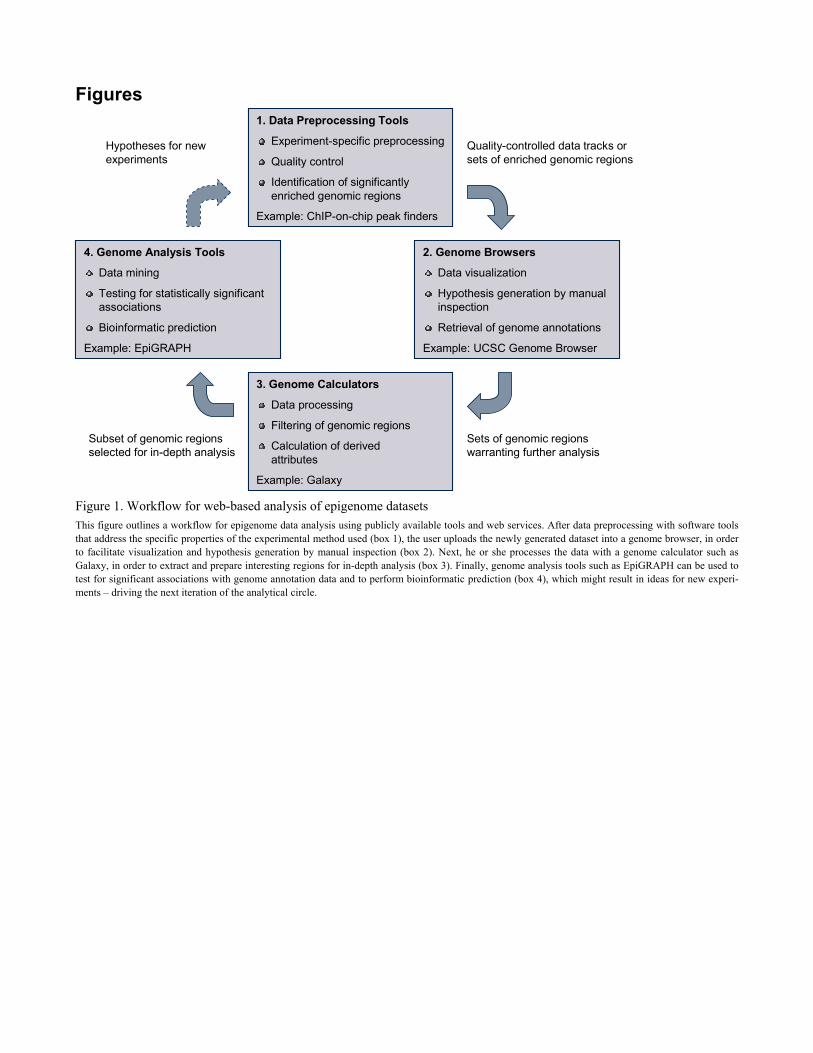
analysis, the first step on EpiGRAPH’s overview page has to be the selection of the genome as-sembly to work on, using the choice box on the right of the page (underneath the EpiGRAPH logo). After selecting human genome assembly “hg18”, we can click the “Define new analysis using this website” button, upon which EpiGRAPH will guide us through a three-step process specifying and launching a new EpiGRAPH analysis. On the first page, we upload a set of genomic regions to be used as input dataset for the Epi-GRAPH analysis (Figure 2). In this case study, a suitable dataset can be obtained simply by clicking the “Show live example” link. This dataset is in tab-separated format, containing one genomic region per row and mandatory columns for chromosome name (e.g. “chr21”) as well as genomic start and end position (e.g. “13998895” and “14000167”). Two non-mandatory col-umns – a unique row identifier (first column) and a binary class attribute (last column) – are al-so included. The class attribute specifies whether or not the respective genomic region is methy-lated, based on an experimental analysis of DNA methylation on chromosome 21 (Yamada, et al., 2004). The input dataset is usually copied and pasted from a text editor or a spreadsheet software into the upload page’s text area (see Note 1 for hints on data preparation), and the con-tent of each column (i.e. whether it contains the chromosome name, chromosome start or end position or additional information) is specified by entering column names or column numbers into the corresponding text fields (as illustrated by the default entries made when clicking the “Show live example link”). In order to continue, we press the “Submit attribute and proceed” button. On the second page, we could specify a control set of genomic regions to which our input data-set should be compared (see Note 2), but since the input dataset already contains two types of regions – methylated and unmethylated CpG islands as specified by the binary class column – we can press the “Skip this step” button and proceed to the next step. On the third page, we specify a number of general settings for the EpiGRAPH analysis (Figure 3): (i) We select which binary class column should be used as the target attribute of the analysis (i.e. for differentiation between positives / cases and negatives / control regions), which is straightforward in our example because the DNA methylation dataset includes only a single class column (“isMethylated”). (ii) We confirm the default settings for down-sampling, a para-meter that is important when working with large datasets (see Note 4). (iii) We select which (epi-) genomic attributes to be included in the analysis. (iv) For documentation purposes we provide a title and a brief textual description of the analysis. In this case study, clicking the

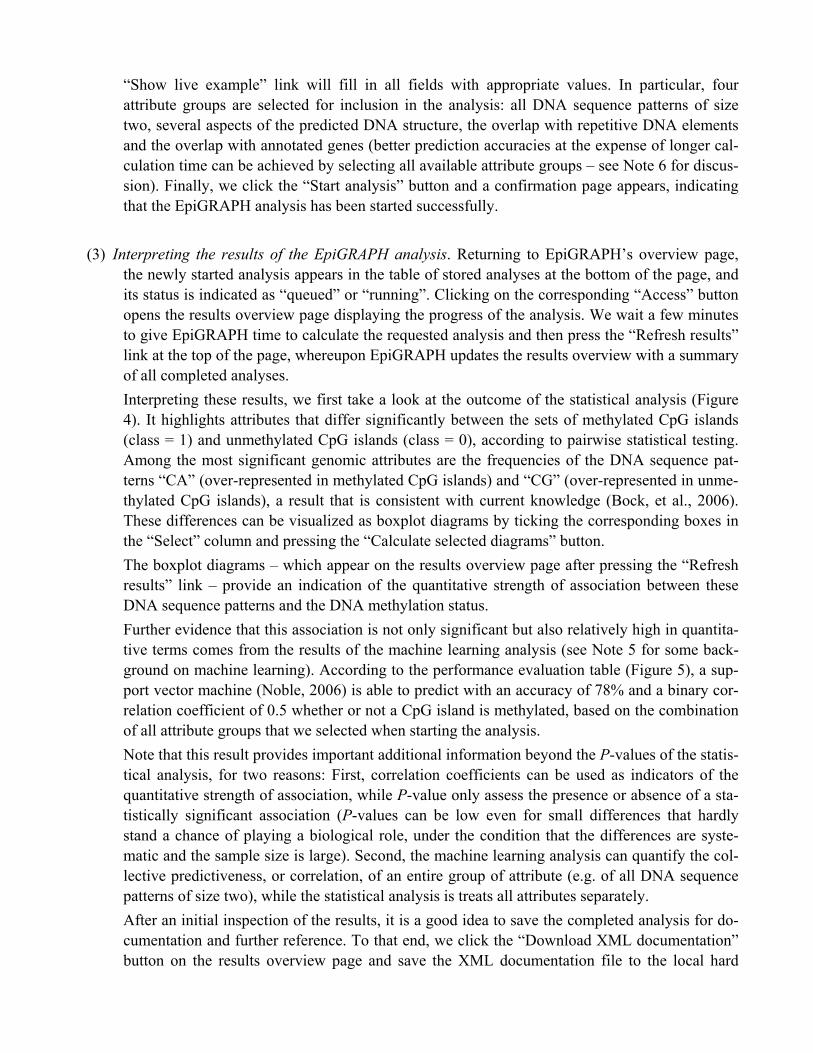
“Show live example” link will fill in all fields with appropriate values. In particular, four attribute groups are selected for inclusion in the analysis: all DNA sequence patterns of size two, several aspects of the predicted DNA structure, the overlap with repetitive DNA elements and the overlap with annotated genes (better prediction accuracies at the expense of longer cal-culation time can be achieved by selecting all available attribute groups – see Note 6 for discus-sion). Finally, we click the “Start analysis” button and a confirmation page appears, indicating that the EpiGRAPH analysis has been started successfully.

(3) Interpreting the results of the EpiGRAPH analysis. Returning to EpiGRAPH’s overview page, the newly started analysis appears in the table of stored analyses at the bottom of the page, and its status is indicated as “queued” or “running”. Clicking on the corresponding “Access” button opens the results overview page displaying the progress of the analysis. We wait a few minutes to give EpiGRAPH time to calculate the requested analysis and then press the “Refresh results” link at the top of the page, whereupon EpiGRAPH updates the results overview with a summary of all completed analyses. Interpreting these results, we first take a look at the outcome of the statistical analysis (Figure 4). It highlights attributes that differ significantly between the sets of methylated CpG islands (class = 1) and unmethylated CpG islands (class = 0), according to pairwise statistical testing. Among the most significant genomic attributes are the frequencies of the DNA sequence pat-terns “CA” (over-represented in methylated CpG islands) and “CG” (over-represented in unme-thylated CpG islands), a result that is consistent with current knowledge (Bock, et al., 2006). These differences can be visualized as boxplot diagrams by ticking the corresponding boxes in the “Select” column and pressing the “Calculate selected diagrams” button. The boxplot diagrams – which appear on the results overview page after pressing the “Refresh results” link – provide an indication of the quantitative strength of association between these DNA sequence patterns and the DNA methylation status. Further evidence that this association is not only significant but also relatively high in quantita-tive terms comes from the results of the machine learning analysis (see Note 5 for some back-ground on machine learning). According to the performance evaluation table (Figure 5), a sup-port vector machine (Noble, 2006) is able to predict with an accuracy of 78% and a binary cor-relation coefficient of 0.5 whether or not a CpG island is methylated, based on the combination of all attribute groups that we selected when starting the analysis. Note that this result provides important additional information beyond the P-values of the statis-tical analysis, for two reasons: First, correlation coefficients can be used as indicators of the quantitative strength of association, while P-value only assess the presence or absence of a sta-tistically significant association (P-values can be low even for small differences that hardly stand a chance of playing a biological role, under the condition that the differences are syste-matic and the sample size is large). Second, the machine learning analysis can quantify the col-lective predictiveness, or correlation, of an entire group of attribute (e.g. of all DNA sequence patterns of size two), while the statistical analysis is treats all attributes separately. After an initial inspection of the results, it is a good idea to save the completed analysis for do-cumentation and further reference. To that end, we click the “Download XML documentation” button on the results overview page and save the XML documentation file to the local hard

disk. This file constitutes a comprehensive account of the analysis settings and of all completed results, providing a suitable basis for sharing an EpiGRAPH analysis with colleagues (e.g. by including it in the supplementary material of a paper).

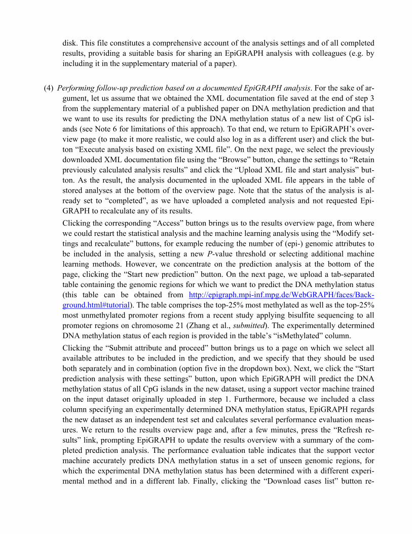
(4) Performing follow-up prediction based on a documented EpiGRAPH analysis. For the sake of ar-

gument, let us assume that we obtained the XML documentation file saved at the end of step 3 from the supplementary material of a published paper on DNA methylation prediction and that we want to use its results for predicting the DNA methylation status of a new list of CpG isl-ands (see Note 6 for limitations of this approach). To that end, we return to EpiGRAPH’s over-view page (to make it more realistic, we could also log in as a different user) and click the but-ton “Execute analysis based on existing XML file”. On the next page, we select the previously downloaded XML documentation file using the “Browse” button, change the settings to “Retain previously calculated analysis results” and click the “Upload XML file and start analysis” but-ton. As the result, the analysis documented in the uploaded XML file appears in the table of stored analyses at the bottom of the overview page. Note that the status of the analysis is al-ready set to “completed”, as we have uploaded a completed analysis and not requested Epi-GRAPH to recalculate any of its results. Clicking the corresponding “Access” button brings us to the results overview page, from where we could restart the statistical analysis and the machine learning analysis using the “Modify set-tings and recalculate” buttons, for example reducing the number of (epi-) genomic attributes to be included in the analysis, setting a new P-value threshold or selecting additional machine learning methods. However, we concentrate on the prediction analysis at the bottom of the page, clicking the “Start new prediction” button. On the next page, we upload a tab-separated table containing the genomic regions for which we want to predict the DNA methylation status (this table can be obtained from http://epigraph.mpi-inf.mpg.de/WebGRAPH/faces/Back-ground.html#tutorial). The table comprises the top-25% most methylated as well as the top-25% most unmethylated promoter regions from a recent study applying bisulfite sequencing to all promoter regions on chromosome 21 (Zhang et al., submitted). The experimentally determined DNA methylation status of each region is provided in the table’s “isMethylated” column. Clicking the “Submit attribute and proceed” button brings us to a page on which we select all available attributes to be included in the prediction, and we specify that they should be used both separately and in combination (option five in the dropdown box). Next, we click the “Start prediction analysis with these settings” button, upon which EpiGRAPH will predict the DNA methylation status of all CpG islands in the new dataset, using a support vector machine trained on the input dataset originally uploaded in step 1. Furthermore, because we included a class column specifying an experimentally determined DNA methylation status, EpiGRAPH regards the new dataset as an independent test set and calculates several performance evaluation meas-ures. We return to the results overview page and, after a few minutes, press the “Refresh re-sults” link, prompting EpiGRAPH to update the results overview with a summary of the com-pleted prediction analysis. The performance evaluation table indicates that the support vector machine accurately predicts DNA methylation status in a set of unseen genomic regions, for which the experimental DNA methylation status has been determined with a different experi-mental method and in a different lab. Finally, clicking the “Download cases list” button re-

trieves a tab-separated table containing individual DNA methylation predictions for each ge-nomic region in the test set.

Genomics analysis using Galaxy (supplemented by Galaxy screencast “Promoters and SNPs”) Galaxy (http://galaxyproject.org/) provides a computational framework that addresses two key chal-lenges of genome analysis, simplicity and reproducibility. It enables bench researchers to rapidly access and analyze enormous datasets without installing or configuring any software. For software en-gineers and computational scientists it provides a zero-configuration development framework that will immediately connect novel or existing analysis tool with their intended target audience – researchers.

(1) A typical task in genomics: Identifying highly polymorphic promoters. The utility of Galaxy is best illustrated by an example. A researcher wants to find human promoters showing evidence of adaptive evolution or relaxation of selective constraint. Such promoters are potentially inter-esting as they may point to genetic causes of human-specific gene expression. As single nucleo-tide polymorphisms (SNPs) are the most common source of genomic variation among the hu-man population (Frazer, et al., 2007), a straightforward approach is to select the promoters that exhibit the highest density of SNPs. Such an analysis would involve the following steps:

1. Obtain gene and SNP annotations for the human genome from the UCSC Table Browser 2. Transform gene annotations into positions of potential promoters by selecting the region lo-

cated 500 base pairs upstream of each gene’s transcription start site 3. Calculate the intersection between each putative promoter and all SNPs 4. Compute the density of SNPs for each promoter region 5. Visualize the genomic vicinity of the ten promoters with highest SNP density

Only the first and last steps can be performed using current genome browsers, while the re-searcher must find or build a custom solution to perform steps 2 through 4. For most experi-mentalists this presents a formidable barrier, preventing them from making effective use of ex-isting datasets. Indeed, coordinates of SNPs are available from the UCSC Table Browser, but this dataset is enormous (millions of data points cannot be loaded into a desktop spreadsheet application) and effectively unusable by experimentalists who lack computational expertise or bioinformatic support. While designing Galaxy we sought to enable experimentalists for per-forming such analysis without the need to install or configure anything.

(2) Using Galaxy to identify highly polymorphic promoters. Consider again the example of looking

for human promoters showing evidence of adaptive evolution or relaxation of constraint. Usual-ly, the initial step of such an analysis would involve downloading the coordinates of all genes and SNPs in the human genome onto one’s personal computer. Next, the user would upload these data to an appropriate analysis tool (provided that it can handle this amount of data). Ob-viously, this procedure is inconvenient and often infeasible, once more highlighting the funda-mental difficulty faced by experimental biologists every day: one first needs to download huge datasets (450 MB in the case of all human SNPs) and then re-uploads the same data to another Internet-based resource (if a suitable web service exists that can perform the analysis online) or install software that can perform the analysis on the local computer. It is much more efficient and practical to implement direct connections between analysis tools and data warehouses, which is what Galaxy does.

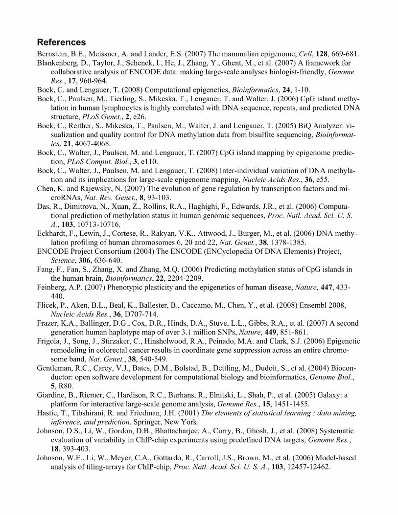
Here, we show how one can perform the search for rapidly evolving promoters using Galaxy (Figure 5). First, we load coordinates of all human RefSeq genes (a conservative set of gene an-notation) and SNPs (dbSNP release 126) into Galaxy using its direct connection to the UCSC Table Browser. Next, we transform coordinates of genes into coordinates of potential promoter regions by taking 500 base pairs immediate upstream on the each gene’s start. We use the cov-erage tool from Galaxy’s “Operate on genomic intervals” tool category to compute the number of SNPs residing in each of the promoters we generated during the previous step. Finally, we use the sort tool and select 100 promoters with the highest number of SNPs. Figure 6 illustrates how all steps of this analysis are documented in Galaxy’s history frame. The history starts from the datasets uploaded from UCSC Genome Browser, which are represented by the two first his-tory items (“1: Human Genes” and “2: SNPs”). A detailed demonstration of this analysis is available as Galaxy screencast “Promoters and SNPs” on the following website: http://galaxy.psu.edu/screencasts.html.

An advanced case study combining the use of Galaxy and EpiGRAPH (supplemented by EpiGRAPH video tutorial 3) In the following case study, we compare the genetic and epigenetic characteristics of highly polymor-phic promoter regions with a control set of promoter regions that contain no more than a single SNP within the kilobase region upstream of the transcription start site of annotated genes. This case study is more complex than the previous two, making use of both Galaxy and EpiGRAPH to address a real-world biological question. Therefore, the following description has to focus on the main concepts, while we refer to video tutorial 3 from EpiGRAPH’s Background page (http://epigraph.mpi-inf.mpg.de/WebGRAPH/faces/Background.html#tutorial) for a step-by-step guide.

(1) Loading SNP and promoter region data into Galaxy. Before we can use EpiGRAPH to identify

genomic and epigenomic differences between polymorphic and non-polymorphic promoter re-gions, it is necessary to derive suitable lists of positives / cases and negatives / control regions. As outlined in the previous section, the Galaxy web service provides us with a convenient solu-tion for performing the necessary calculations online. In the first step, we load two sets of ge-nomic regions from the UCSC Genome Browser into Galaxy, namely the genomic coordinates of all SNPs from the dbSNP database and the putative promoter regions of RefSeq-annotated genes (for practical reasons, the latter were defined as the kilobase region upstream of the anno-tated transcription start site). To increase the speed of calculation, we limit our analysis to a 1% subset of the human genome known as the ENCODE regions (ENCODE Project Consortium, 2004), although it would well be possible to perform the same analysis genome-wide. The video tutorial demonstrates two different ways in which data can be loaded into Galaxy, the first one being initiated from the UCSC Genome Browser and the second one initiated from within Ga-laxy (the effect of both methods is identical: the dataset becomes available for further processing in Galaxy).

(2) Using Galaxy to derive sets of highly polymorphic and non-polymorphic promoter regions. Inside

Galaxy, it is now possible to derive two sets of promoter regions, one comprising all regions that contain at least ten SNPs (to be used as positives) and the other comprising all regions that contain zero or one SNPs (to be used as negatives). Several generic functions are successively

applied to complete this task. First, a region-based join is calculated between the set of promo-ter regions and the set of SNP positions, giving rise to a list containing all possible pairs of a promoter region and a SNP that overlap with each other. Second, the count function is used to quantify the number of times that a specific promoter region occurs in this list. Third, the result-ing list is filtered according to the minimum or maximum SNP threshold (one and ten), respec-tively. Fourth, an identifier-based join with the original list of promoter regions is performed in order to recover the positional information that was lost during the counting step.

(3) Specifying and launching an EpiGRAPH analysis on polymorphic promoter data. Upon comple-

tion of the Galaxy analysis, we copy the resulting tab-separated tables of positives (highly po-lymorphic promoter regions) and negatives (non-polymorphic promoter regions) to spreadsheet software and change a few column names for better readability, before pasting the data into a new EpiGRAPH analysis. The EpiGRAPH analysis is created as described in the first case study (see above), with two major differences. First, the sets of positives and negatives are up-loaded as two different datasets on the first and second page of EpiGRAPH’s analysis specifica-tion workflow, rather than being combined in a single input dataset and distinguished by a bi-nary class column. Second, the current analysis includes all ten attribute groups that are availa-ble by default for the human genome assembly hg18, namely: (i) DNA sequence, (ii) DNA structure, (iii) repetitive DNA, (iv) chromosome organization, (v) evolutionary history, (vi) population variation, (vii) genes, (viii) regulatory regions, (ix) transcriptome, and (x) epige-nome and chromatin structure. As a result, calculation by EpiGRAPH takes substantially longer and it is highly recommended to switch on e-mail notification before starting the analysis.

(4) Interpreting the results of the EpiGRAPH analysis. After receiving an e-mail notification inform-

ing us about successful completion of the analysis, we click the direct link given in the e-mail, which logs us in automatically and opens the results overview page. Our inspection starts with a quick look at the results of the machine learning analysis. These results quantify how well Epi-GRAPH could predict the target class from each of the ten attribute groups. In other words, they provide a measure for the combined predictiveness of each attribute group for whether or not a specific promoter region is highly polymorphic. Reassuringly, the prediction performance is close to perfect for the “population variation” attribute group, which includes SNP data (96% prediction accuracy and a binary correlation of 0.92 between predictions and actual values). In addition to this expected result, a number of interesting attribute groups score highly, including “regulatory regions” and “epigenome and chromatin structure”. An inspection of the results of the statistical analysis confirms this observation. While SNP-related attributes are again the most discriminatory features, there is also a clear tendency of non-polymorphic promoter re-gions being associated with regulatory elements such as bona fide CpG islands (Bock, et al., 2007) and conserved transcription factor binding sites, while they are depleted in terms of re-combination hotspots. As a follow-up analysis, it would be interesting to analyze whether the enrichment for bona fide CpG islands and transcription factor binding sites is a side effect of an elevated degree of evolu-tionary conservation among non-polymorphic promoters or whether it constitutes a separate ef-fect with an independent biological cause. Two options are available to address this question.

First, we could restart the machine learning analysis with modified settings, assessing whether the combined predictiveness of the attribute groups “regulatory regions” and “evolutionary his-tory” exceeds the predictiveness of “evolutionary history” alone (the latter group contains all conservation-related attributes). Second, we could click the “Download data table” button, download the table containing all calculated attribute values for all genomic regions included in the analysis, load this data table into a statistics software (such as R) and construct linear mod-els in order to assess the significance of attributes from the “regulatory regions” group after sta-tistically correcting for evolutionary conservation of the promoter region.

Notes (1) Data preparation from diverse sources. Epigenome analysis frequently incorporates genomic re-

gion data from a number of sources (collaboration partners, the supplementary material of pub-lished papers, output files of data preprocessing software, etc.), which come in a variety of for-mats (tab-separated or comma-separated tables, genome browser tracks, Excel sheets, etc.). Therefore, data preparation is an important step and requires caution and experience to prevent errors that could invalidate all subsequent analyses. From our experience, the following tools can significantly facilitate data preparation: (i) The liftOver utility of the UCSC Genome Browser (http://genome.ucsc.edu/cgi-bin/hgLiftOver) maps genomic coordinates from one ge-nome assembly to another, e.g. from human genome hg17 to hg18. (ii) Advanced text editors provide various features for text file formatting, such as column-based editing and support for regular expressions when performing complex search-and-replace operations (a practical intro-duction into regular expressions is available from http://analyser.oli.tudelft.nl/regex/). (iii) Add-ing, removing and rearranging columns as well as cosmetic changes (e.g. renaming columns) is often done easiest within spreadsheet software, before saving the final table in tab-separated format or copying and pasting it directly into EpiGRAPH.

(2) Deriving an appropriate control set. For the two EpiGRAPH case studies presented in this paper,

the choice of an appropriate control set is obvious: unmethylated CpG islands complement me-thylated CpG islands and non-polymorphic promoter regions complement highly polymorphic promoter regions. However, for many applications a control set must be derived by random sampling of genomic regions, which requires careful correction for potential confounding fac-tors. Assume that we want to analyze the epigenetic characteristics of preferred retroviral inte-gration sites (i.e. genomic regions at which viruses such as HIV are incorporated into the host DNA), based on sequenced integration sites (Wang, et al., 2007). We will have to make sure that the control set does not contain more repetitive regions than the set of integration sites, be-cause the latter dataset is artificially biased against repetitive regions, and this should be reflect-ed in the control set. Furthermore, we may want to adjust the control set for the GC content of the genomic regions (which is a strong predictor for a wide range of genomic properties), in or-der to pick up more subtle differences. EpiGRAPH’s attribute submission page provides func-tionality to derive “fair” random control sets. On the one hand, the chromosomal distribution and region-length distribution of the input dataset can be exactly matched by the control set; on the other hand, any deviation in terms of GC content, repeat content and exon overlap can be limited to a pre-defined maximum.

(3) Working with custom attributes. EpiGRAPH enables the user to define custom attributes that can

be used in the same ways as the default attributes, i.e. not only as input datasets to be analyzed with EpiGRAPH, but also as prediction attributes for inclusion in the analysis of other datasets. The upload page for defining a new custom attribute can be accessed using the “Upload custom attribute dataset” button on EpiGRAPH’s overview page. It looks essentially identical to the attribute submission step when launching an EpiGRAPH analysis. Three ways of defining a custom attributes are available: (i) to upload the attribute data in tab-separated format, as we did in the two EpiGRAPH case studies above (e.g. useful for incorporating custom experimental data); (ii) to derive the new attribute from a source attribute that is already contained in Epi-GRAPH’s database (either by default or as a custom attribute), specifying a filter criterion and a formula defining an additional column that is to be calculated by EpiGRAPH (e.g. useful for re-trieving the DNA sequences of a set of genomic regions); (iii) to request calculation of a matched control attribute for a given source attribute (e.g. useful when the same set of control regions are to be used in multiple EpiGRAPH analyses). All custom attributes are exclusively available to the user under whose account they were created. It is, however, possible to down-load a custom attribute in XML format and share this file with other researchers, who can then upload it into their own EpiGRAPH user accounts.

(4) Working with large datasets. Genome analysis with Galaxy and EpiGRAPH can be performed on

large datasets. However, analyses take longer and have to be planned more carefully when data-sets are large. (i) It is usually advisable to perform a pilot study on a small subset of the dataset of interest before going large-scale. For this purpose, EpiGRAPH provides functionality to down-sample datasets to a given size. (ii) The increase in prediction accuracy gained by includ-ing more than 1,000 genomic regions in the input dataset of an EpiGRAPH analysis is usually low and rarely worth the additional calculation time. (iii) From our experience, Mozilla Firefox is the web browser that is most tolerant toward cutting and pasting large sets of genomic regions into text areas on a web page. (iv) To process large tables with spreadsheet software, Microsoft Excel 2007 is often the best choice because it supports tables with up to 1,048,576 rows and up to 16,384 columns, while the limits of other spreadsheets are substantially lower and often in-sufficient. (v) It is rarely a good idea to submit more than five analyses in parallel to any given web service, and it is advisable to contact the scientists who operate the web service for advice before starting extremely large analyses.

(5) Understanding the basics of machine learning. EpiGRAPH’s machine learning analysis uses

classification algorithms such as support vector machines and logistic regression models in or-der to assess the predictiveness of entire groups of attributes for a class value of interest. To that end, it tries to predict whether a given genomic region is likely to belong to the set of positives or negatives, based on different combinations of prediction attributes. Technically, machine learning algorithms are methods for estimating or approximating a mathematical function that links the values of several (known) prediction attributes to a prediction of the (unknown) class value. The estimating function is learnt from a training dataset and its performance is evaluated on a test dataset. Because data is frequently scarce, EpiGRAPH applies a strategy called cross-

validation to perform classifier training and testing on the same dataset – splitting it into ten partitions, training on nine partitions and testing on the tenth partition and repeating this process ten times. An important concern when using machine learning methods is the risk of over-training, i.e. the danger that the classification algorithm “remembers” individual cases rather than learning generalizable concepts, which leads to over-optimistic prediction accuracies that are not sustainable on new datasets. While EpiGRAPH is implemented in a way that the risk of over-training is low, potential error sources remain (such as re-running the machine learning analysis based only on the top-scoring attributes from the statistical analysis) and it is recom-mended to consult further background texts on machine learning and / or discuss with an expe-rienced bioinformatician before drawing far-reaching conclusions from the results of Epi-GRAPH’s machine learning analysis. A good practical introduction into machine learning is provided by Witten and Frank (Witten and Frank, 2000), while Hastie et al. (Hastie, et al., 2001) provide a more mathematical treatment. Further references are given by Tarca et al. in a recent primer on machine learning methods (Tarca, et al., 2007).

(6) Understanding DNA methylation prediction. In this paper, we have used DNA methylation data

to illustrate epigenome prediction with EpiGRAPH. While the use of support vector machines for predicting the DNA methylation status of CpG islands is well-established (Bock, et al., 2006; Fang, et al., 2006), it is not recommended to use predictions calculated with the classifier from the first case study for any real applications, for two reasons: First, the dataset used for training the classifier is small and restricted to chromosome 21, while genome-scale datasets are now available as training data. Second, the prediction is based on only a small subset of relevant attributes, although it is known that additional attributes groups – such as more complex DNA sequence patterns – can increase prediction accuracy. To obtain more realistic DNA methyla-tion predictions, EpiGRAPH should be applied to a larger and more representative DNA methy-lation dataset (e.g. Meissner, et al., 2008) and all of EpiGRAPH’s default attributes should be included in the prediction. Alternatively, a pre-calculated genome-wide map of CpG island strength prediction can be used, which we derived previously (Bock, et al., 2007) and which is available from http://neighborhood.bioinf.mpi-inf.mpg.de/CpG_islands_revisited (the higher a CpG island’s predicted strength, the less likely it is methylated).

Acknowledgements We would like to thank Joachim Büch for maintaining the IT infrastructure of EpiGRAPH, Yoichi Yamada and Sascha Tierling for providing DNA methylation data and Martina Paulsen as well as Jörn Walter for helpful discussions. EpiGRAPH is partially funded by the European Union through the CANCERDIP project (HEALTH-F2-2007-200620; http://www.cancerdip.eu/). Galaxy is supported by NSF Grant DBI-0543285 and NIH Grant 5R01HG003646-02 as well as by funds from the Huck Insti-tutes for Life Sciences at Penn State University and Pennsylvania Department of Health.

Competing interests The authors declare that no competing financial interests exist.

Figures

2. Genome Browsers

Data visualization

Hypothesis generation by manual inspection

Retrieval of genome annotations

Example: UCSC Genome Browser

2. Genome Browsers

Data visualization

Hypothesis generation by manual inspection

Retrieval of genome annotations

Example: UCSC Genome Browser

4. Genome Analysis Tools

Data mining

Testing for statistically significant associations

Bioinformatic prediction

Example: EpiGRAPH

4. Genome Analysis Tools

Data mining

Testing for statistically significant associations

Bioinformatic prediction

Example: EpiGRAPH

3. Genome Calculators

Data processing

Filtering of genomic regions

Calculation of derived attributes

Example: Galaxy

3. Genome Calculators

Data processing

Filtering of genomic regions

Calculation of derived attributes

Example: Galaxy

1. Data Preprocessing Tools

Experiment-specific preprocessing

Quality control

Identification of significantly enriched genomic regions

Example: ChIP-on-chip peak finders

1. Data Preprocessing Tools

Experiment-specific preprocessing

Quality control

Identification of significantly enriched genomic regions

Example: ChIP-on-chip peak finders

Quality-controlled data tracks or sets of enriched genomic regions

Hypotheses for new experiments

Sets of genomic regions warranting further analysis

Subset of genomic regions selected for in-depth analysis

Figure 1. Workflow for web-based analysis of epigenome datasets This figure outlines a workflow for epigenome data analysis using publicly available tools and web services. After data preprocessing with software tools that address the specific properties of the experimental method used (box 1), the user uploads the newly generated dataset into a genome browser, in order to facilitate visualization and hypothesis generation by manual inspection (box 2). Next, he or she processes the data with a genome calculator such as Galaxy, in order to extract and prepare interesting regions for in-depth analysis (box 3). Finally, genome analysis tools such as EpiGRAPH can be used to test for significant associations with genome annotation data and to perform bioinformatic prediction (box 4), which might result in ideas for new experi-ments – driving the next iteration of the analytical circle.

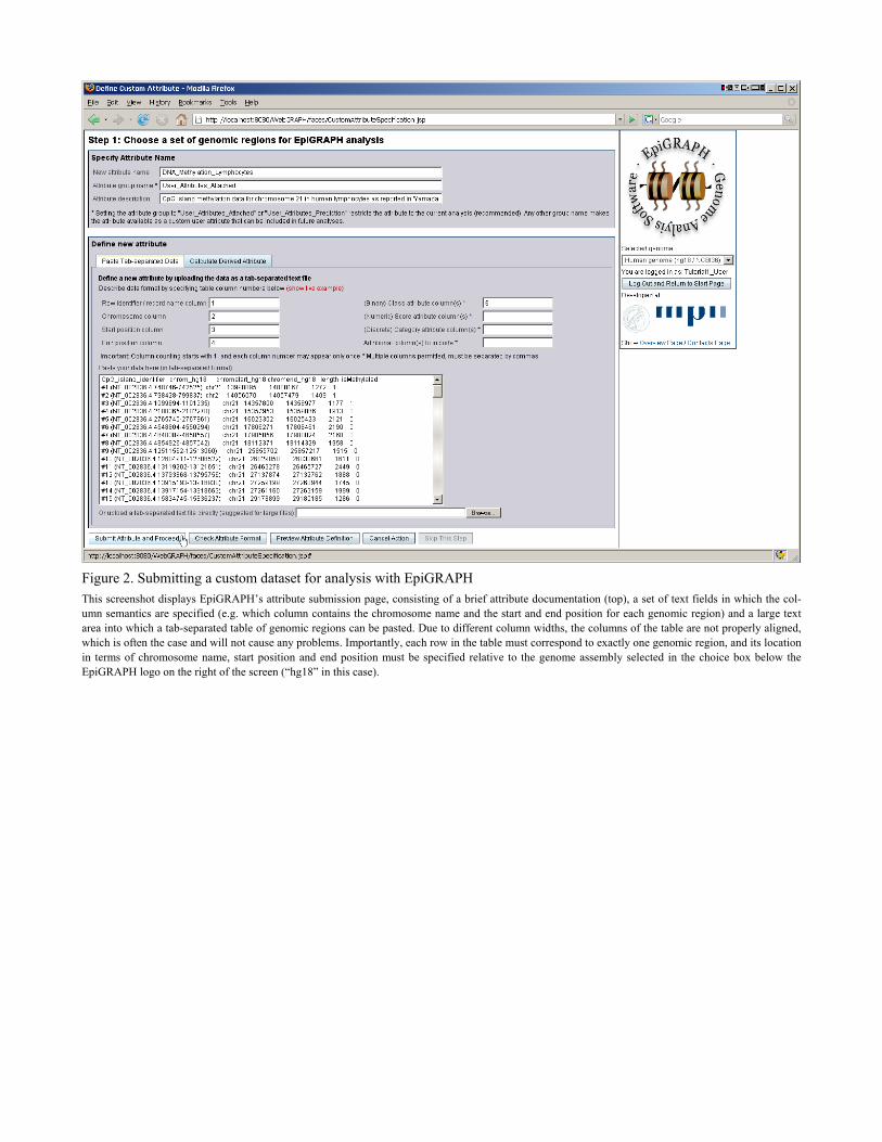
Figure 2. Submitting a custom dataset for analysis with EpiGRAPH This screenshot displays EpiGRAPH’s attribute submission page, consisting of a brief attribute documentation (top), a set of text fields in which the col-umn semantics are specified (e.g. which column contains the chromosome name and the start and end position for each genomic region) and a large text area into which a tab-separated table of genomic regions can be pasted. Due to different column widths, the columns of the table are not properly aligned, which is often the case and will not cause any problems. Importantly, each row in the table must correspond to exactly one genomic region, and its location in terms of chromosome name, start position and end position must be specified relative to the genome assembly selected in the choice box below the EpiGRAPH logo on the right of the screen (“hg18” in this case).

Figure 3. Configuring and starting an EpiGRAPH analysis This screenshot displays EpiGRAPH’s analysis specification page. Here, the user can select which class attribute to use (if more than one class attribute was provided during the attribute submission steps), configure down-sampling, select prediction attributes and enter a brief documentation of the analysis.

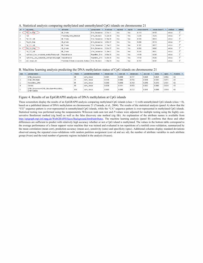
A. Statistical analysis comparing methylated and unmethylated CpG islands on chromosome 21

B. Machine learning analysis predicting the DNA methylation status of CpG islands on chromosome 21

Figure 4. Results of an EpiGRAPH analysis of DNA methylation at CpG islands These screenshots display the results of an EpiGRAPH analysis comparing methylated CpG islands (class = 1) with unmethylated CpG islands (class = 0), based on a published dataset of DNA methylation on chromosome 21 (Yamada, et al., 2004). The results of the statistical analysis (panel A) show that the “CG” sequence pattern is over-represented in unmethylated CpG islands, while the “CA” sequence pattern is over-represented in methylated CpG islands. Statistical testing was performed using the nonparametric Wilcoxon rank-sum test and P-values were adjusted for multiple testing using the highly con-servative Bonferroni method (sig bonf) as well as the false discovery rate method (sig fdr). An explanation of the attribute names is available from http://epigraph.mpi-inf.mpg.de/WebGRAPH/faces/Background.html#attributes. The machine learning analysis (panel B) confirms that these and other differences are sufficient to predict with relatively high accuracy whether or not a CpG island is methylated. The values in the bottom table correspond to the average performance of a linear support vector machine that was trained and evaluated in ten repetitions of a tenfold cross-validation, summarized by the mean correlation (mean corr), prediction accuracy (mean acc), sensitivity (sens) and specificity (spec). Additional columns display standard deviations observed among the repeated cross-validations with random partition assignment (corr sd and acc sd), the number of attribute variables in each attribute group (#vars) and the total number of genomic regions included in the analysis (#cases).

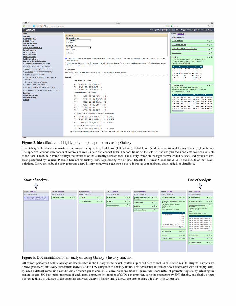
Figure 5. Identification of highly polymorphic promoters using Galaxy The Galaxy web interface consists of four areas: the upper bar, tool frame (left column), detail frame (middle column), and history frame (right column). The upper bar contains user account controls as well as help and contact links. The tool frame on the left lists the analysis tools and data sources available to the user. The middle frame displays the interface of the currently selected tool. The history frame on the right shows loaded datasets and results of ana-lyses performed by the user. Pictured here are six history items representing two original datasets (1: Human Genes and 2: SNP) and results of their mani-pulations. Every action by the user generates a new history item, which can then be used in subsequent analyses, downloaded, or visualized.

Figure 6. Documentation of an analysis using Galaxy’s history function All actions performed within Galaxy are documented in the history frame, which contains uploaded data as well as calculated results. Original datasets are always preserved, and every subsequent analysis adds a new entry into the history frame. This screenshot illustrates how a user starts with an empty histo-ry, adds a dataset containing coordinates of human genes and SNPs, converts coordinates of genes into coordinates of promoter regions by selecting the region located 500 base pairs upstream of each gene, computes the number of SNPs per promoter, sorts the promoters by SNP density, and finally selects 100 top regions. In addition to documenting analyses, Galaxy’s history frame allows the user to share a history with colleagues.

References Bernstein, B.E., Meissner, A. and Lander, E.S. (2007) The mammalian epigenome, Cell, 128, 669-681. Blankenberg, D., Taylor, J., Schenck, I., He, J., Zhang, Y., Ghent, M., et al. (2007) A framework for

collaborative analysis of ENCODE data: making large-scale analyses biologist-friendly, Genome Res., 17, 960-964.

Bock, C. and Lengauer, T. (2008) Computational epigenetics, Bioinformatics, 24, 1-10. Bock, C., Paulsen, M., Tierling, S., Mikeska, T., Lengauer, T. and Walter, J. (2006) CpG island methy-

lation in human lymphocytes is highly correlated with DNA sequence, repeats, and predicted DNA structure, PLoS Genet., 2, e26.

Bock, C., Reither, S., Mikeska, T., Paulsen, M., Walter, J. and Lengauer, T. (2005) BiQ Analyzer: vi-sualization and quality control for DNA methylation data from bisulfite sequencing, Bioinformat-ics, 21, 4067-4068.

Bock, C., Walter, J., Paulsen, M. and Lengauer, T. (2007) CpG island mapping by epigenome predic-tion, PLoS Comput. Biol., 3, e110.

Bock, C., Walter, J., Paulsen, M. and Lengauer, T. (2008) Inter-individual variation of DNA methyla-tion and its implications for large-scale epigenome mapping, Nucleic Acids Res., 36, e55.

Chen, K. and Rajewsky, N. (2007) The evolution of gene regulation by transcription factors and mi-croRNAs, Nat. Rev. Genet., 8, 93-103.

Das, R., Dimitrova, N., Xuan, Z., Rollins, R.A., Haghighi, F., Edwards, J.R., et al. (2006) Computa-tional prediction of methylation status in human genomic sequences, Proc. Natl. Acad. Sci. U. S. A., 103, 10713-10716.

Eckhardt, F., Lewin, J., Cortese, R., Rakyan, V.K., Attwood, J., Burger, M., et al. (2006) DNA methy-lation profiling of human chromosomes 6, 20 and 22, Nat. Genet., 38, 1378-1385.

ENCODE Project Consortium (2004) The ENCODE (ENCyclopedia Of DNA Elements) Project, Science, 306, 636-640.

Fang, F., Fan, S., Zhang, X. and Zhang, M.Q. (2006) Predicting methylation status of CpG islands in the human brain, Bioinformatics, 22, 2204-2209.

Feinberg, A.P. (2007) Phenotypic plasticity and the epigenetics of human disease, Nature, 447, 433-440.

Flicek, P., Aken, B.L., Beal, K., Ballester, B., Caccamo, M., Chen, Y., et al. (2008) Ensembl 2008, Nucleic Acids Res., 36, D707-714.

Frazer, K.A., Ballinger, D.G., Cox, D.R., Hinds, D.A., Stuve, L.L., Gibbs, R.A., et al. (2007) A second generation human haplotype map of over 3.1 million SNPs, Nature, 449, 851-861.

Frigola, J., Song, J., Stirzaker, C., Hinshelwood, R.A., Peinado, M.A. and Clark, S.J. (2006) Epigenetic remodeling in colorectal cancer results in coordinate gene suppression across an entire chromo-some band, Nat. Genet., 38, 540-549.

Gentleman, R.C., Carey, V.J., Bates, D.M., Bolstad, B., Dettling, M., Dudoit, S., et al. (2004) Biocon-ductor: open software development for computational biology and bioinformatics, Genome Biol., 5, R80.

Giardine, B., Riemer, C., Hardison, R.C., Burhans, R., Elnitski, L., Shah, P., et al. (2005) Galaxy: a platform for interactive large-scale genome analysis, Genome Res., 15, 1451-1455.

Hastie, T., Tibshirani, R. and Friedman, J.H. (2001) The elements of statistical learning : data mining, inference, and prediction. Springer, New York.

Johnson, D.S., Li, W., Gordon, D.B., Bhattacharjee, A., Curry, B., Ghosh, J., et al. (2008) Systematic evaluation of variability in ChIP-chip experiments using predefined DNA targets, Genome Res., 18, 393-403.

Johnson, W.E., Li, W., Meyer, C.A., Gottardo, R., Carroll, J.S., Brown, M., et al. (2006) Model-based analysis of tiling-arrays for ChIP-chip, Proc. Natl. Acad. Sci. U. S. A., 103, 12457-12462.

Karolchik, D., Kuhn, R.M., Baertsch, R., Barber, G.P., Clawson, H., Diekhans, M., et al. (2008) The UCSC Genome Browser Database: 2008 update, Nucleic Acids Res., 36, D773-779.

Kumaki, Y., Oda, M. and Okano, M. (2008) QUMA: quantification tool for methylation analysis, Nucleic Acids Res.

Liu, F., Tostesen, E., Sundet, J.K., Jenssen, T.K., Bock, C., Jerstad, G.I., et al. (2007) The human ge-nomic melting map, PLoS Comput. Biol., 3, e93.

Liu, X.S. (2007) Getting started in tiling microarray analysis, PLoS Comput. Biol., 3, 1842-1844. Meissner, A., Mikkelsen, T.S., Gu, H., Wernig, M., Hanna, J., Sivachenko, A., et al. (2008) Genome-

scale DNA methylation maps of pluripotent and differentiated cells, Nature, 454, 766-770. Moser, D., Ekawardhani, S., Kumsta, R., Palmason, H., Bock, C., Athanassiadou, Z., et al. (2008)

Functional Analysis of a Potassium-Chloride Co-Transporter 3 (SLC12A6) Promoter Polymor-phism Leading to an Additional DNA Methylation Site, Neuropsychopharmacology.

Noble, W.S. (2006) What is a support vector machine?, Nat. Biotechnol., 24, 1565-1567. Pond, S.L., Frost, S.D. and Muse, S.V. (2005) HyPhy: hypothesis testing using phylogenies, Bioinfor-

matics, 21, 676-679. Rice, P., Longden, I. and Bleasby, A. (2000) EMBOSS: the European Molecular Biology Open Soft-

ware Suite, Trends Genet., 16, 276-277. Schones, D.E. and Zhao, K. (2008) Genome-wide approaches to studying chromatin modifications,

Nat. Rev. Genet., 9, 179-191. Tarca, A.L., Carey, V.J., Chen, X.W., Romero, R. and Draghici, S. (2007) Machine learning and its

applications to biology, PLoS Comput. Biol., 3, e116. van Steensel, B. (2005) Mapping of genetic and epigenetic regulatory networks using microarrays, Nat.

Genet., 37 Suppl, S18-24. Wang, G.P., Ciuffi, A., Leipzig, J., Berry, C.C. and Bushman, F.D. (2007) HIV integration site selec-

tion: analysis by massively parallel pyrosequencing reveals association with epigenetic modifica-tions, Genome Res., 17, 1186-1194.

Williams, R.B., Chan, E.K., Cowley, M.J. and Little, P.F. (2007) The influence of genetic variation on gene expression, Genome Res., 17, 1707-1716.

Witten, I.H. and Frank, E. (2000) Data mining : practical machine learning tools and techniques with Java implementations. Morgan Kaufmann, San Francisco, Calif.

Yamada, Y., Watanabe, H., Miura, F., Soejima, H., Uchiyama, M., Iwasaka, T., et al. (2004) A com-prehensive analysis of allelic methylation status of CpG islands on human chromosome 21q, Ge-nome Res., 14, 247-266.

Zhang, M.Q. (2005) Computational molecular biology of genome expression and regulation. In Pal, S.K. (ed), PReMI. Springer-Verlag Berlin Heidelberg, 31-38.