Weather Research Forecast Version 3.8 Meteorological …WRF is a next-generation mesoscale numerical weather prediction system designed to serve both operational forecasting and atmospheric

Weather Research Forecast Version 3.8 Meteorological Model Evaluation

Annual 2015 12-km CONUS

Prepared for: US EPA

Prepared by:

UNC-Chapel Hill

September 16, 2016

September 2016 UNC-EMAQ(4-07)-008.v1 i

CONTENTS

EXECUTIVE SUMMARY .................................................................................................... ES-1

1.0 INTRODUCTION .......................................................................................................... 1-1

2.0 WRF MODEL CONFIGURATION .................................................................................... 2-2

3.0 MODEL PERFORMANCE EVALUATION APPROACH ....................................................... 3-7

4.0 WRF MODEL PERFORMANCE EVALATUION RESULTS.................................................. 4-11

Model Evaluation Results for 2-m Temperature .............................................................. 4-11

Model Evaluation Results for 2-m Mixing Ratio ............................................................... 4-20

Model Evaluation Results for 10-m Wind Speed .............................................................. 4-29

Model Evaluation Results for 10-m Wind Direction ......................................................... 4-38

Model Evaluation Results for Monthly Precipitation ....................................................... 4-48

January Precipitation 2015 ............................................................................................... 4-48

February Precipitation 2015 ............................................................................................. 4-48

March Precipitation 2015 ................................................................................................. 4-49

April Precipitation 2015 .................................................................................................... 4-49

May Precipitation 2015 ..................................................................................................... 4-49

June Precipitation 2015 .................................................................................................... 4-50

July Precipitation 2015 ...................................................................................................... 4-50

August Precipitation 2015 ................................................................................................ 4-50

September Precipitation 2015 .......................................................................................... 4-51

October Precipitation 2015............................................................................................... 4-51

November Precipitation 2015 ........................................................................................... 4-51

December Precipitation 2015 ........................................................................................... 4-52

Model Evaluation Results for Solar Radiation .................................................................. 4-65

5.0 ADDITIONAL RESULTS ............................................................................................... 5-67

TABLES

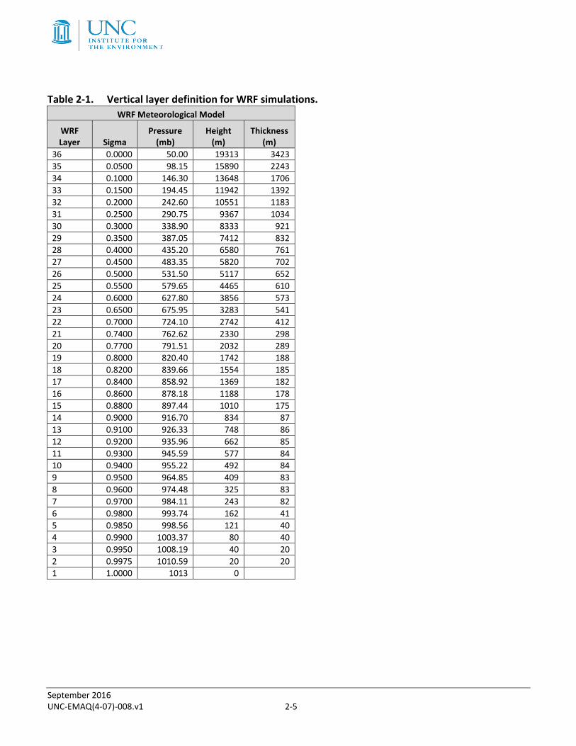
Table 2-1. Vertical layer definition for WRF simulations. .................................................... 2-5

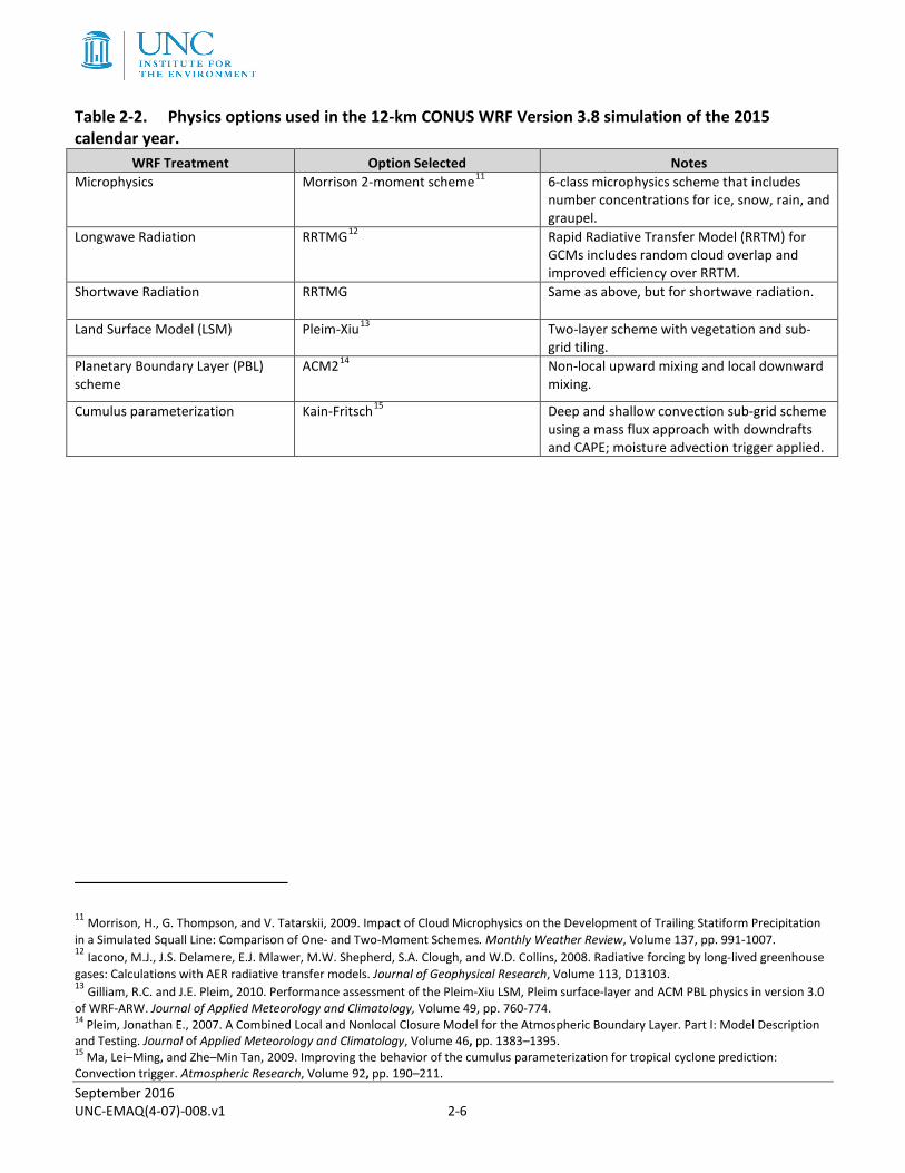
Table 2-2. Physics options used in the 12-km CONUS WRF Version 3.8 simulation of the 2015 calendar year. .................................................................................. 2-6

September 2016 UNC-EMAQ(4-07)-008.v1 ii

FIGURES

Figure 2-1. 12-km CONUS WRF modeling domain. ............................................................... 2-4

Figure 3-1. Locations of MADIS surface meteorological modeling sites with the WRF 12-km CONUS modeling domain. ............................................................... 3-9

Figure 3-2. Location of SURFRAD (top) and ISIS (bottom) radiation monitors. ...................... 3-10

Figure 4-1. Soccer plot of monthly 2-m temperature error and bias averaged over the 12-km CONUS domain for the 2015 calendar year. ................................... 4-12

Figure 4-2. Diurnal 2-m temperature error and bias (°C) averaged over the 12-km CONUS domain for January (top) and July (bottom) 2015. .............................. 4-13

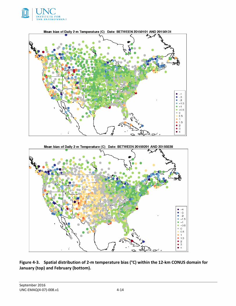
Figure 4-3. Spatial distribution of 2-m temperature bias (°C) within the 12-km CONUS domain for January (top) and February (bottom). ............................... 4-14

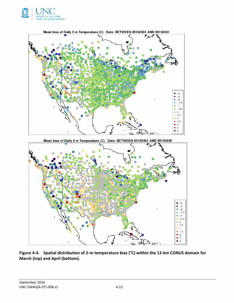
Figure 4-4. Spatial distribution of 2-m temperature bias (°C) within the 12-km CONUS domain for March (top) and April (bottom). ........................................ 4-15

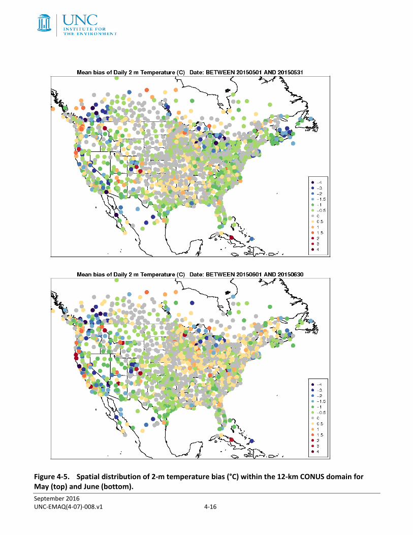
Figure 4-5. Spatial distribution of 2-m temperature bias (°C) within the 12-km CONUS domain for May (top) and June (bottom). ........................................... 4-16

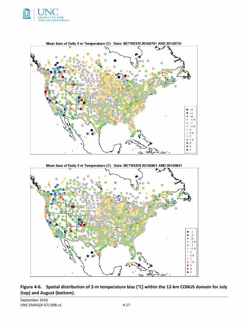
Figure 4-6. Spatial distribution of 2-m temperature bias (°C) within the 12-km CONUS domain for July (top) and August (bottom). ......................................... 4-17

Figure 4-7. Spatial distribution of 2-m temperature bias (°C) within the 12-km CONUS domain for September (top) and October (bottom). ........................... 4-18

Figure 4-8. Spatial distribution of 2-m temperature bias (°C) within the 12-km CONUS domain for November (top) and December (bottom). ........................ 4-19

Figure 4-9. Soccer plot of monthly 2-m mixing ratio error and bias (g/kg) averaged over the 12-km CONUS domain for the 2015 calendar year. ........................... 4-21

Figure 4-10. Diurnal 2-m mixing ratio error and bias (g/kg) averaged over the 12-km CONUS domain for January (top) and July (bottom) 2015. .............................. 4-22

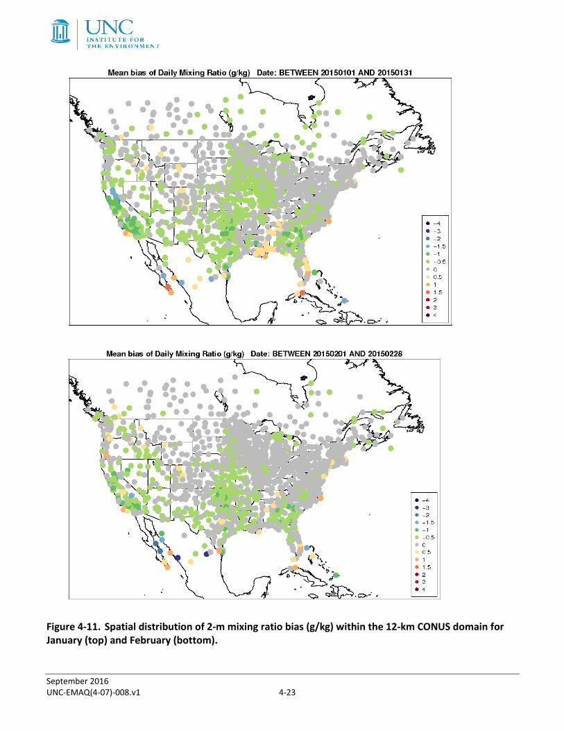
Figure 4-11. Spatial distribution of 2-m mixing ratio bias (g/kg) within the 12-km CONUS domain for January (top) and February (bottom). ............................... 4-23

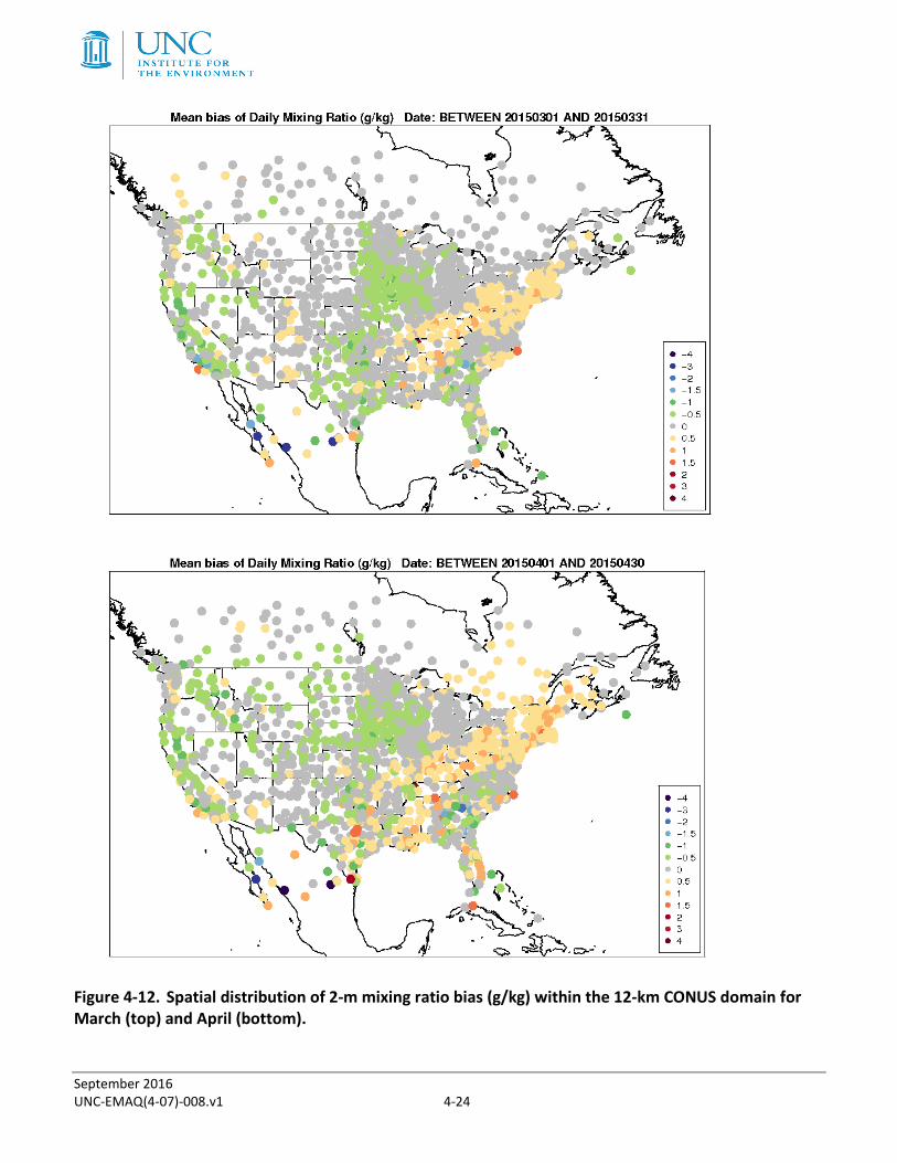
Figure 4-12. Spatial distribution of 2-m mixing ratio bias (g/kg) within the 12-km CONUS domain for March (top) and April (bottom). ........................................ 4-24

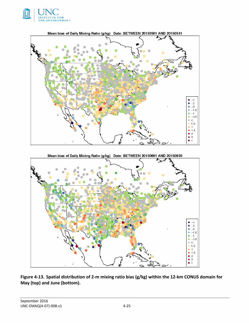
Figure 4-13. Spatial distribution of 2-m mixing ratio bias (g/kg) within the 12-km CONUS domain for May (top) and June (bottom). ........................................... 4-25

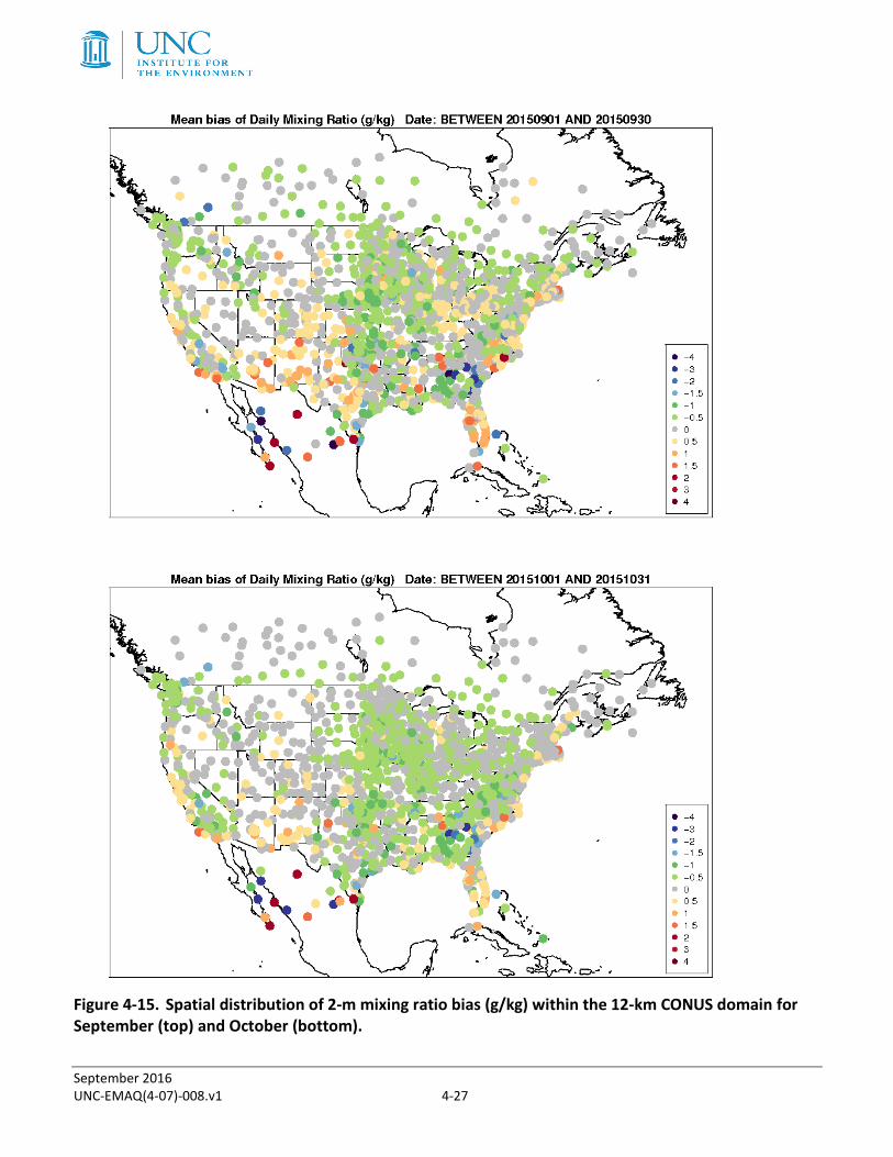
Figure 4-15. Spatial distribution of 2-m mixing ratio bias (g/kg) within the 12-km CONUS domain for September (top) and October (bottom). ........................... 4-27

September 2016 UNC-EMAQ(4-07)-008.v1 iii

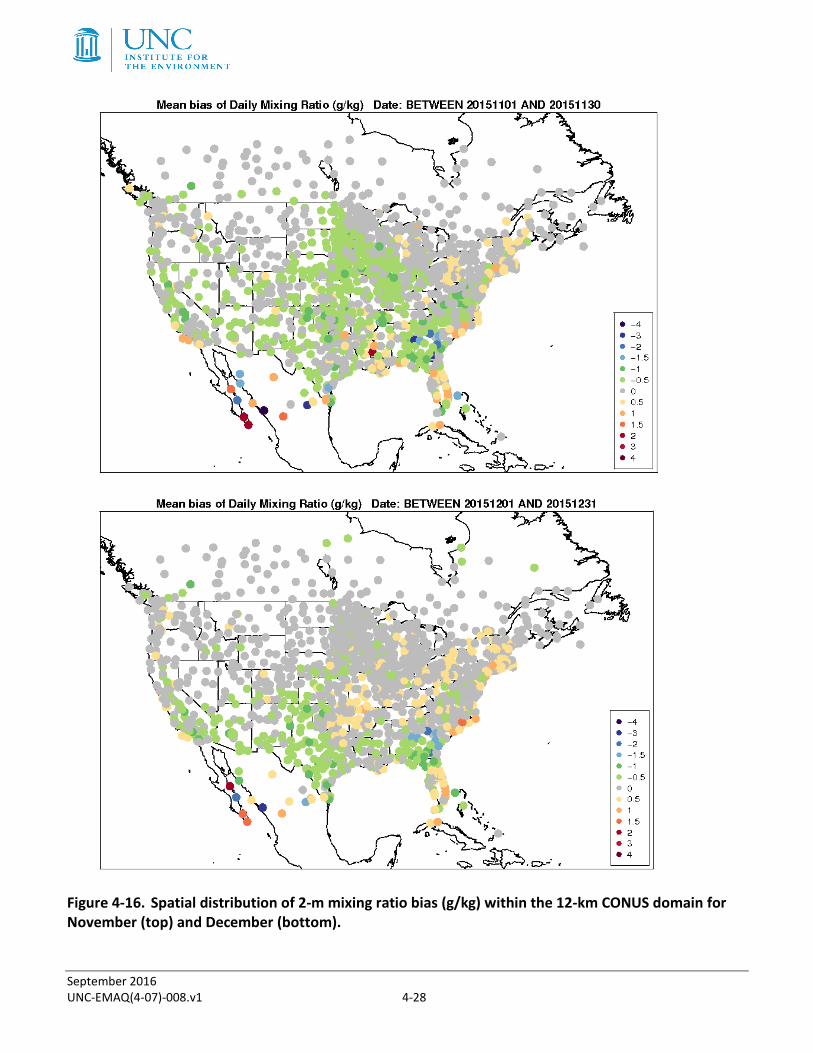
Figure 4-16. Spatial distribution of 2-m mixing ratio bias (g/kg) within the 12-km CONUS domain for November (top) and December (bottom). ........................ 4-28

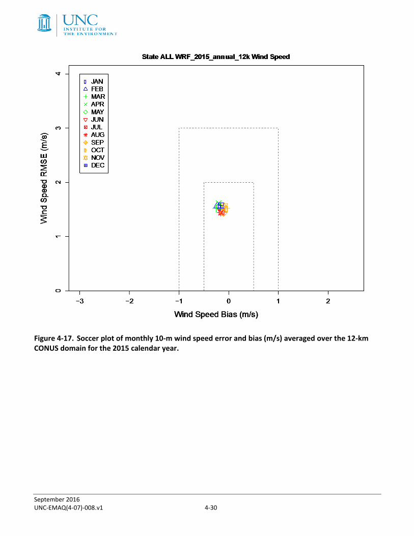
Figure 4-17. Soccer plot of monthly 10-m wind speed error and bias (m/s) averaged over the 12-km CONUS domain for the 2015 calendar year. ........................... 4-30

Figure 4-18. Diurnal 10-m wind speed error and bias (m/s) averaged over the 12-km CONUS domain for January (top) and July (bottom) 2015. ........................ 4-31

Figure 4-19. Spatial distribution of 10-m wind speed bias (m/s) within the 12-km CONUS domain for January (top) and February (bottom). ............................... 4-32

Figure 4-21. Spatial distribution of 10-m wind speed bias (m/s) within the 12-km CONUS domain for May (top) and June (bottom). ........................................... 4-34

Figure 4-25. Soccer plot of monthly 10-m wind direction error and bias averaged over the 12-km CONUS domain for the 2015 calendar year. ........................... 4-39

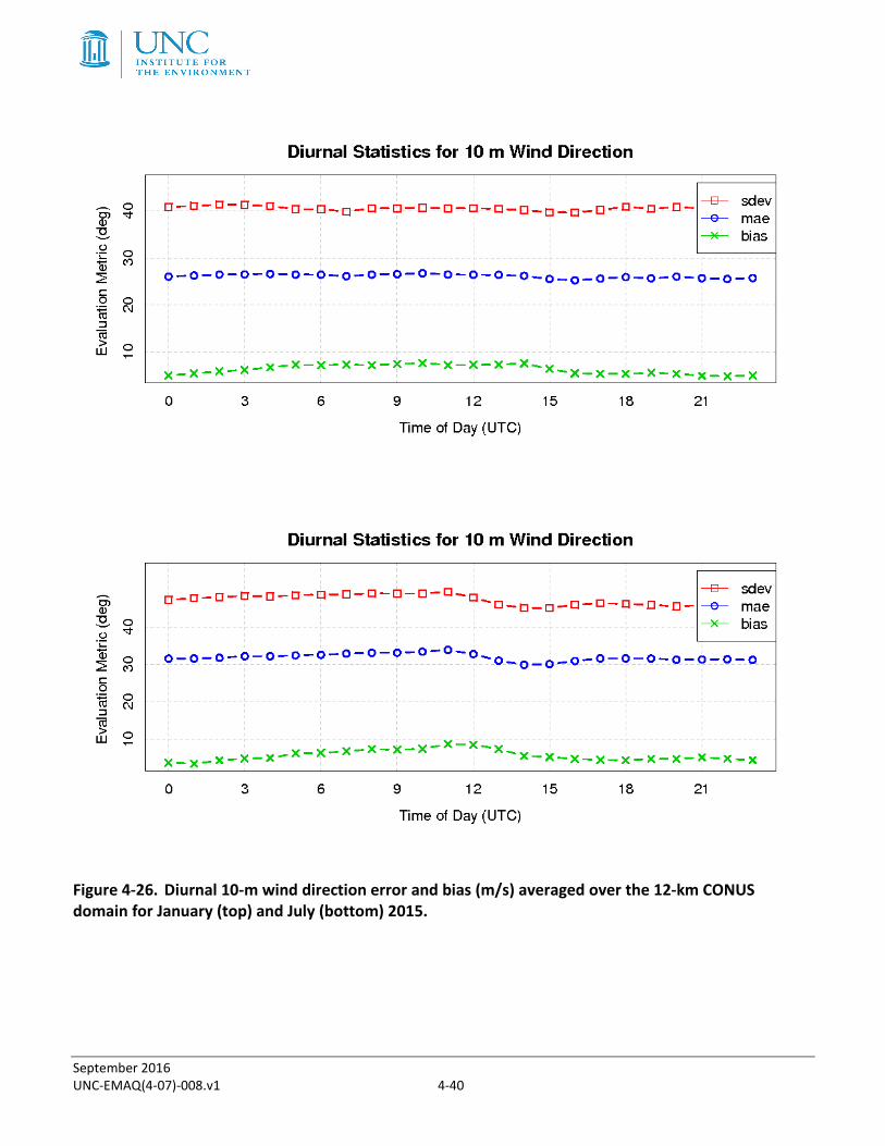
Figure 4-26. Diurnal 10-m wind direction error and bias (m/s) averaged over the 12-km CONUS domain for January (top) and July (bottom) 2015. ................... 4-40

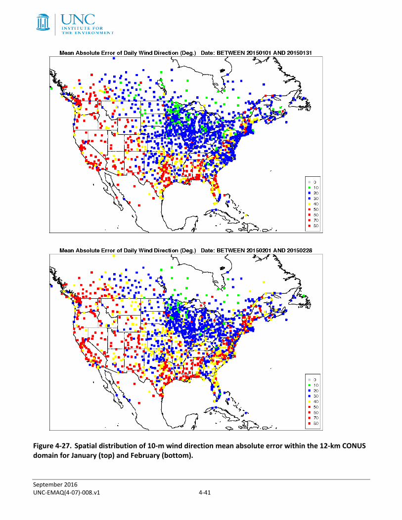
Figure 4-27. Spatial distribution of 10-m wind direction mean absolute error within the 12-km CONUS domain for January (top) and February (bottom). ............. 4-41

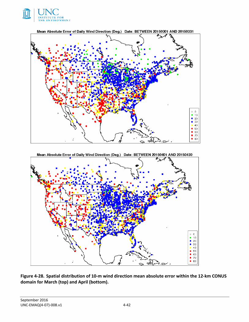
Figure 4-28. Spatial distribution of 10-m wind direction mean absolute error within the 12-km CONUS domain for March (top) and April (bottom). ...................... 4-42

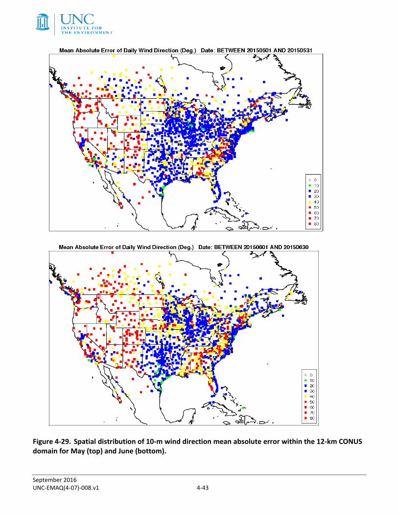
Figure 4-29. Spatial distribution of 10-m wind direction mean absolute error within the 12-km CONUS domain for May (top) and June (bottom). .......................... 4-43

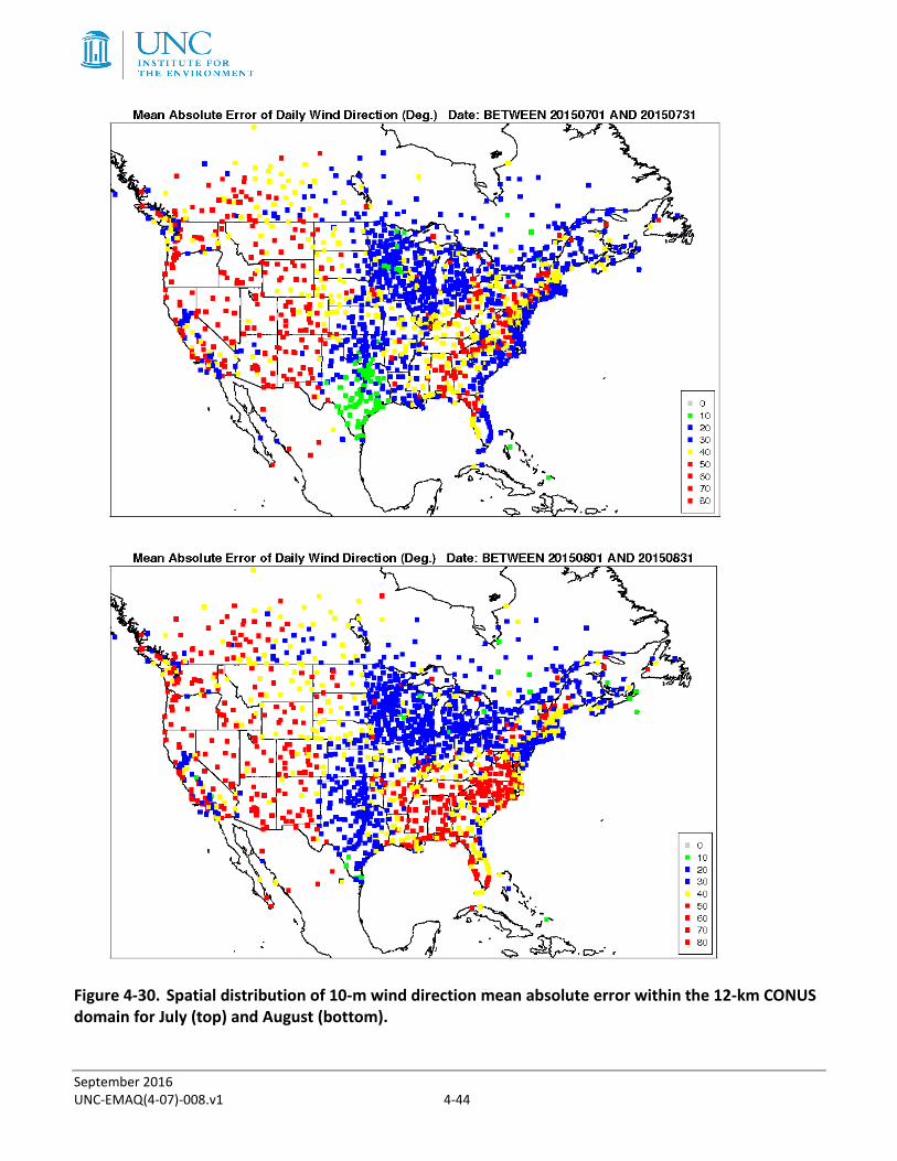
Figure 4-30. Spatial distribution of 10-m wind direction mean absolute error within the 12-km CONUS domain for July (top) and August (bottom). ....................... 4-44

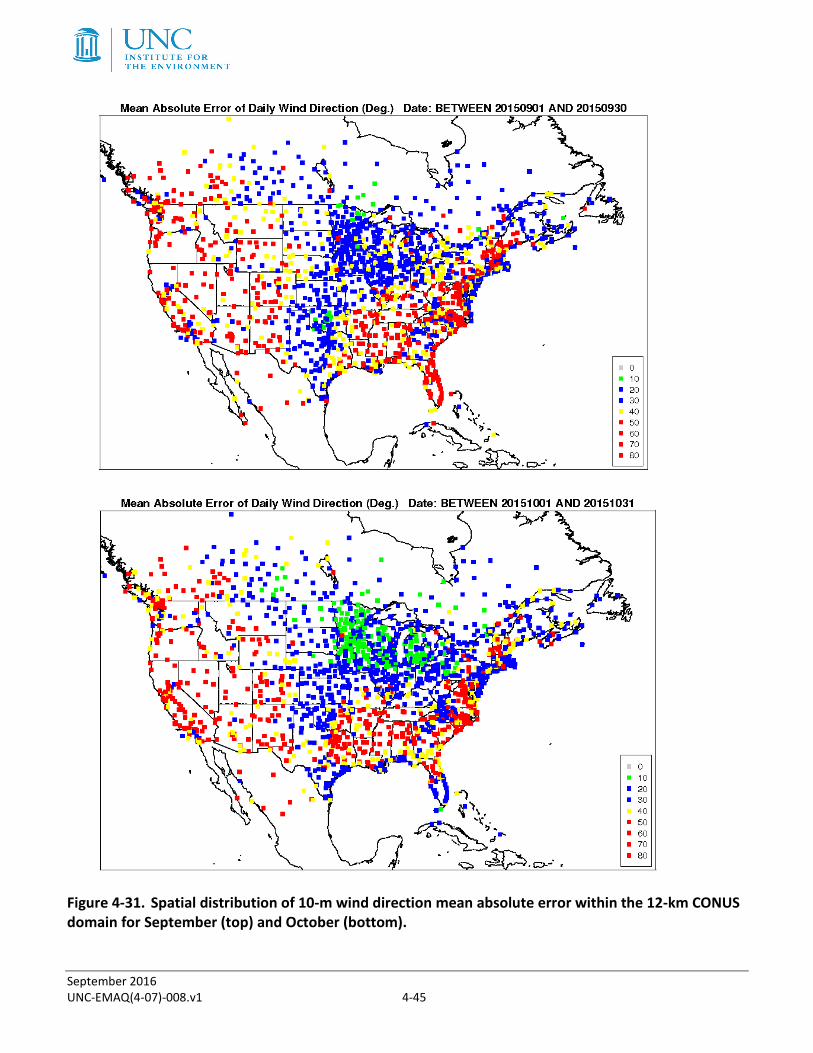
Figure 4-31. Spatial distribution of 10-m wind direction mean absolute error within the 12-km CONUS domain for September (top) and October (bottom). ......... 4-45

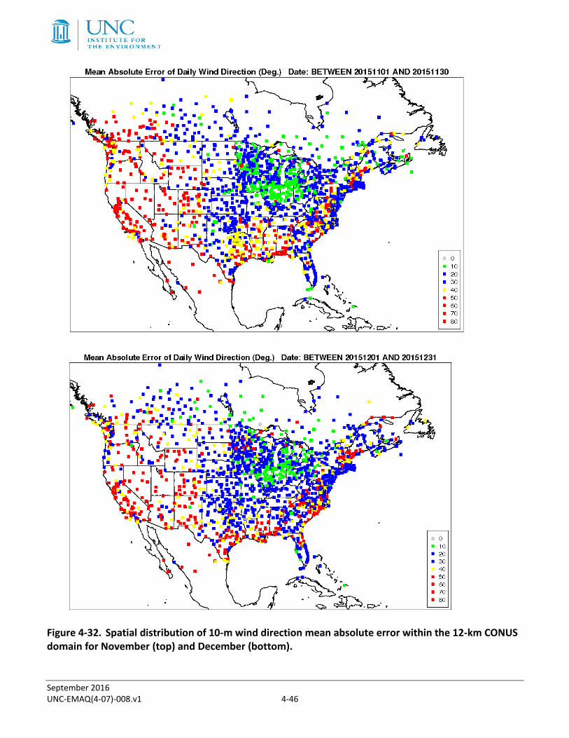
Figure 4-32. Spatial distribution of 10-m wind direction mean absolute error within the 12-km CONUS domain for November (top) and December (bottom). ........................................................................................................... 4-46

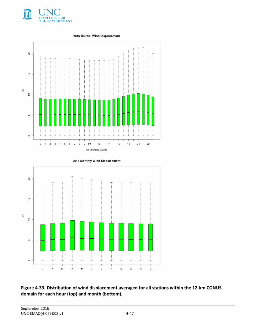
Figure 4-33. Distribution of wind displacement averaged for all stations within the 12-km CONUS domain for each hour (top) and month (bottom). .................... 4-47

Figure 4-34. Comparison of monthly total precipitation (inches) from PRISM (top) and WRF (middle) and WRF minus PRISM (bottom) for the 12-km CONUS domain in January 2015........................................................................ 4-53

Figure 4-35. Comparison of monthly total precipitation (inches) from PRISM (top) and WRF (middle) and WRF minus PRISM (bottom) for the 12-km CONUS domain in February 2015. .................................................................... 4-54

September 2016 UNC-EMAQ(4-07)-008.v1 iv

Figure 4-36. Comparison of monthly total precipitation (inches) from PRISM (top) and WRF (middle) and WRF minus PRISM (bottom) for the 12-km CONUS domain in March 2015.......................................................................... 4-55

Figure 4-37. Comparison of monthly total precipitation (inches) from PRISM (top) and WRF (middle) and WRF minus PRISM (bottom) for the 12-km CONUS domain in April 2015. ........................................................................... 4-56

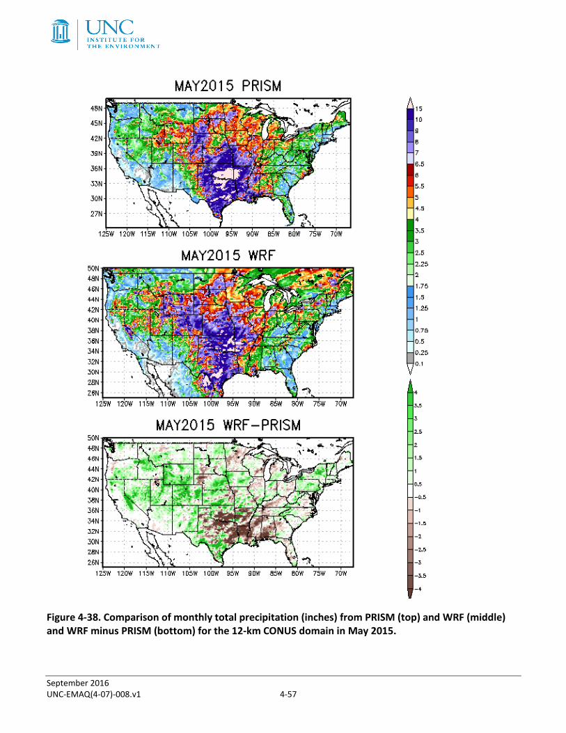
Figure 4-38. Comparison of monthly total precipitation (inches) from PRISM (top) and WRF (middle) and WRF minus PRISM (bottom) for the 12-km CONUS domain in May 2015. ............................................................................ 4-57

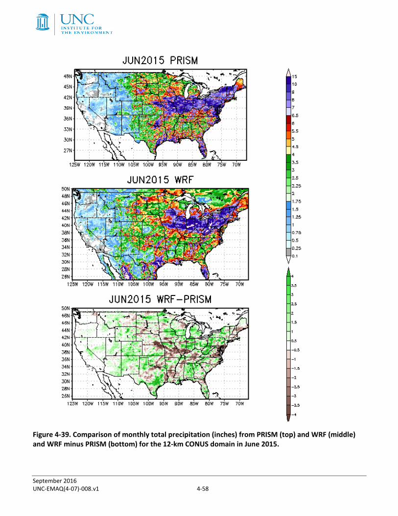
Figure 4-39. Comparison of monthly total precipitation (inches) from PRISM (top) and WRF (middle) and WRF minus PRISM (bottom) for the 12-km CONUS domain in June 2015. ............................................................................ 4-58

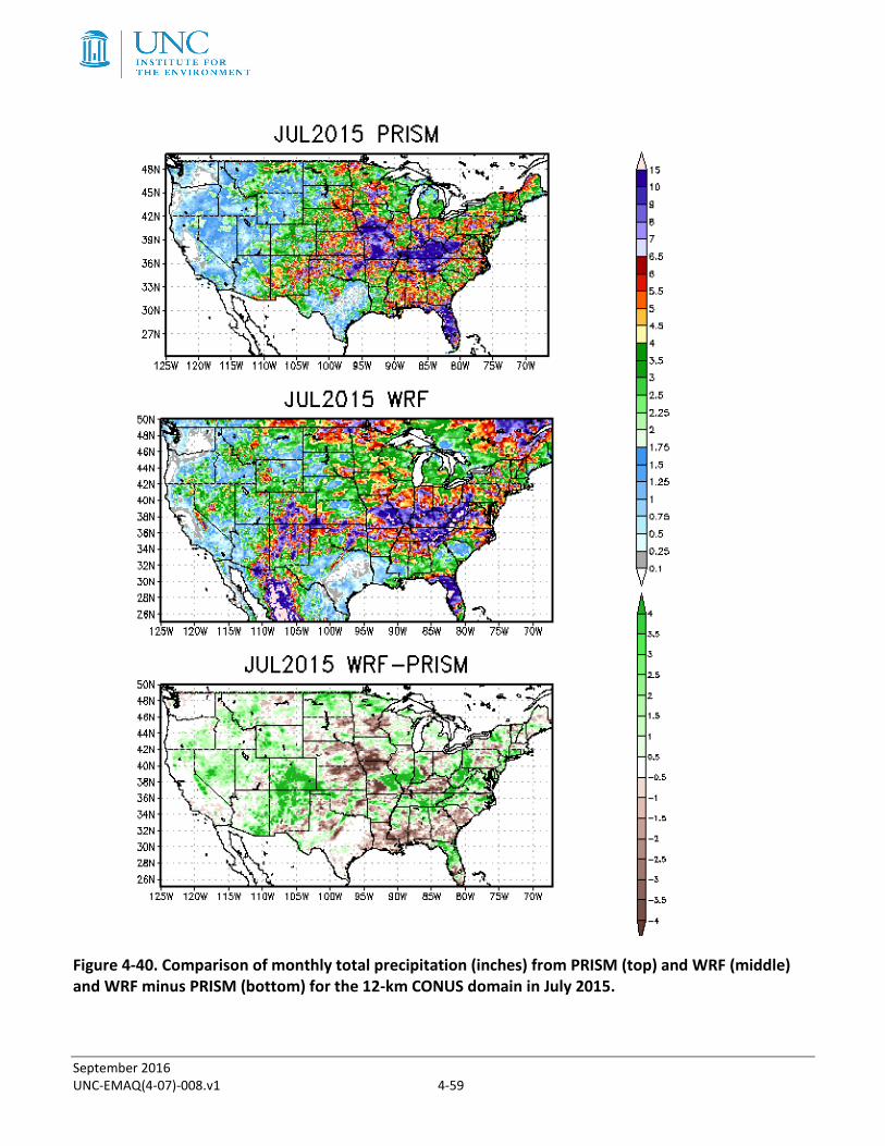
Figure 4-40. Comparison of monthly total precipitation (inches) from PRISM (top) and WRF (middle) and WRF minus PRISM (bottom) for the 12-km CONUS domain in July 2015. ............................................................................. 4-59

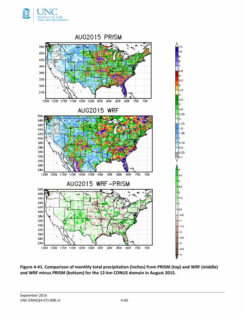
Figure 4-41. Comparison of monthly total precipitation (inches) from PRISM (top) and WRF (middle) and WRF minus PRISM (bottom) for the 12-km CONUS domain in August 2015. ........................................................................ 4-60

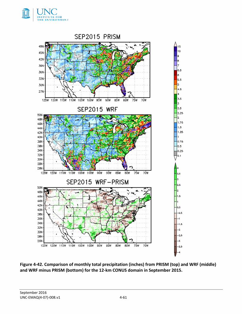
Figure 4-42. Comparison of monthly total precipitation (inches) from PRISM (top) and WRF (middle) and WRF minus PRISM (bottom) for the 12-km CONUS domain in September 2015. ................................................................. 4-61

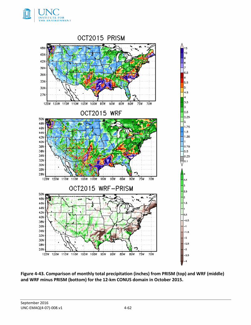
Figure 4-43. Comparison of monthly total precipitation (inches) from PRISM (top) and WRF (middle) and WRF minus PRISM (bottom) for the 12-km CONUS domain in October 2015. ...................................................................... 4-62

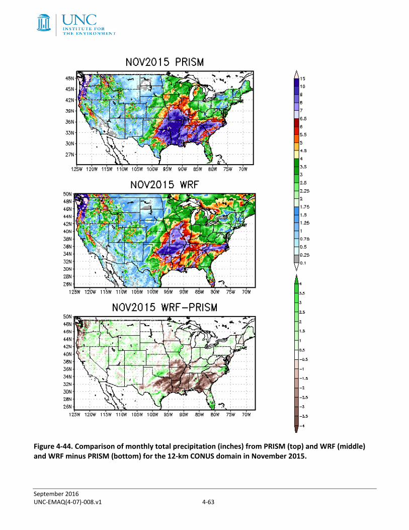
Figure 4-44. Comparison of monthly total precipitation (inches) from PRISM (top) and WRF (middle) and WRF minus PRISM (bottom) for the 12-km CONUS domain in November 2015. .................................................................. 4-63

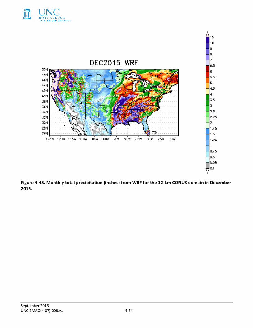
Figure 4-45. Monthly total precipitation (inches) from WRF (middle) for the 12-km CONUS domain in December 2015. .................................................................. 4-64

Figure 4-46. Model bias of shortwave radiation averaged over all SURFRAD and ISIS network monitors within the 12-km CONUS domain for each hour (top) and month (bottom). ................................................................................ 4-66

A-1-1

1.0 INTRODUCTION The University of North Carolina (UNC) at Chapel Hill simulated annual meteorology for the 2015 calendar year to support emissions, photochemical, and dispersion modeling applications for this year. The simulated meteorological data will be used to support assessments of ozone, PM2.5, visibility, and a variety of toxics.

The annual meteorology was simulated using the Weather Research and Forecasting model (WRF) at a 12-km horizontal resolution for the continental United States (CONUS). The WRF meteorological fields were processed using the Meteorology Chemistry Interface Process (MCIP) to generate Community Multiscale Air Quality (CMAQ)-ready input files. Additionally, the 2015 WRF meteorological fields were processed using the Mesoscale Model Interface Tool (MMIF) to generate input files for dispersion models. This report provides technical details about the WRF model configuration and the meteorological model performance evaluation for the 2015 calendar, which includes performance evaluation of 2-m temperature, 2-m mixing ratio, 10-m wind speed and direction, and accumulated monthly precipitation.

September 2016 UNC-EMAQ(4-07)-008.v1 2-2

2.0 WRF MODEL CONFIGURATION We used the Weather Research and Forecasting (WRF) model with the Advanced Research dynamic solver for this meteorological modeling study.1 WRF is a next-generation mesoscale numerical weather prediction system designed to serve both operational forecasting and atmospheric research needs. WRF contains separate modules to compute different physical processes, such as surface energy budgets and soil interactions, turbulence, cloud microphysics, and atmospheric radiation. Within WRF, the user has many options for selecting the different schemes for each type of physical process. There is a WRF Preprocessing System (WPS) that generates the initial and boundary conditions used by WRF, based on topographic datasets, land use information, and larger-scale atmospheric and oceanic models. Below, we outline the model setup, model input, and options (e.g. parameterizations) that were used for the 2015 WRF simulations. The WRF options were selected based on numerical meteorological modeling research and the experience of scientists at the U.S. Environmental Protection Agency (USEPA), within the Office of Research and Development (ORD).2,3,4

A summary of the WRF input data preparation procedure used for this annual modeling exercise is provided below.

Model Selection: The publicly available version of WRF (version 3.8) was used for the 2015 meteorological simulation. This was the latest version of WRF available at the time the simulation was performed. WPS version 3.8 was also used to develop the model inputs.

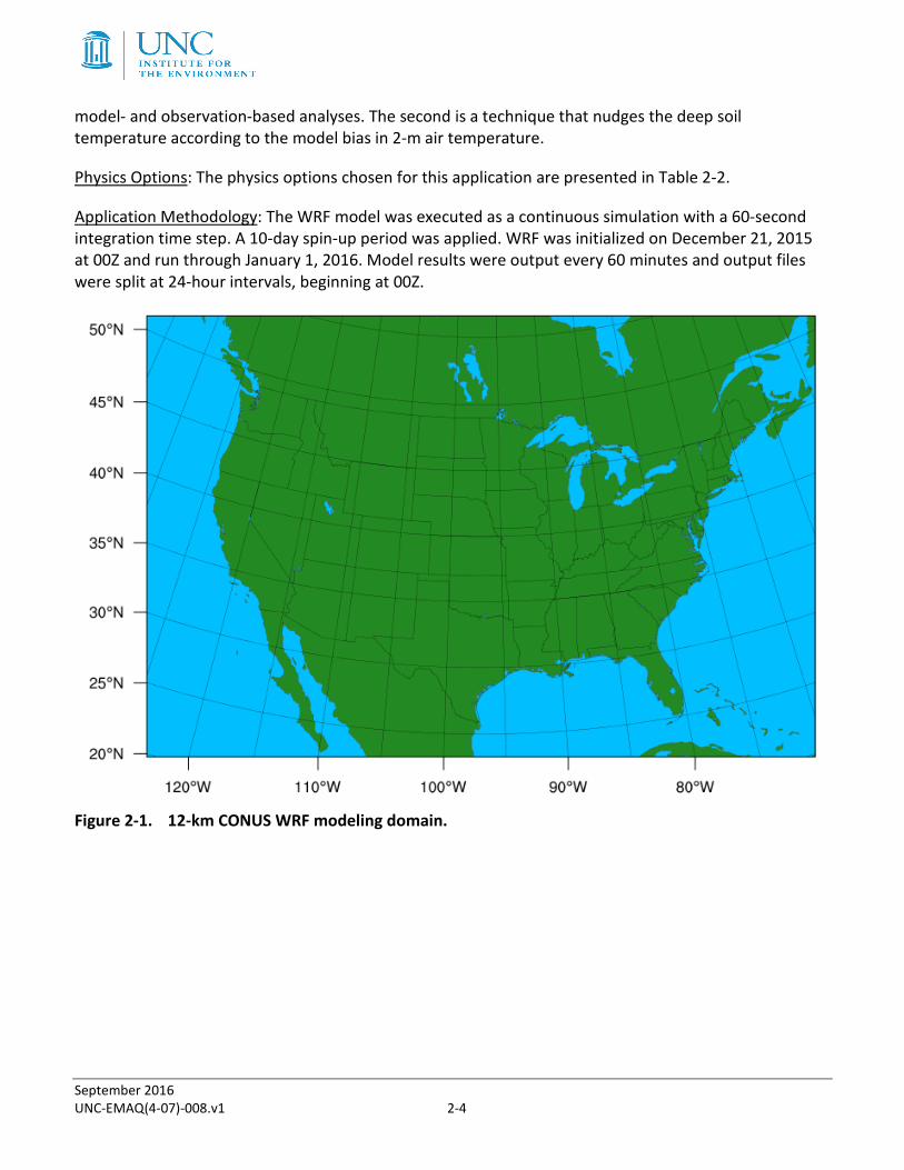
Horizontal Domain Definition: The WRF 12-km configuration includes a 5-grid cell buffer in all directions to minimize any potential numeric noise along WRF domain boundaries, which can affect the air quality model meteorological inputs. Such numeric noise can occur near the boundaries of the WRF domain solution as the boundary conditions come into balance with the WRF numerical algorithms. The WRF horizontal domains are presented in Figure 2-1. The grid projection was Lambert Conformal with a pole of projection of 40 degrees north, -97 degrees east, and standard parallels of 33 and 45 degrees.

Vertical Domain Definition: The WRF modeling was based on 36 vertical layers with a surface layer approximately 20 meters deep. The vertical domain is presented in both sigma and approximate height coordinates in Table 2-1.

Topographic Inputs: Topographic information for the WRF model was developed using the standard WRF terrain databases. The 12-km CONUS domain was based on the latest USGS GMTED2010 data.5 This is 30-second (~900 m) data and replaces the old topography data (GTOPO30) available in prior WRF releases. 1 Skamarock, W.C. and J.B. Klemp, 2008. A time-split nonhydrostatic atmospheric model for weather research and forecasting applications. Journal of Computation Physics, Volume 227, pp. 3465-3485. 2 Pleim, J.E. and R.C. Gilliam, 2009. An indirect data assimilation scheme for deep soil temperature in the Pleim-Xiu land surface model. Journal of Applied Meteorology and Climatology, Volume 48, pp. 1362-1376. 3Gilliam, R.C. and J.E. Pleim, 2010. Performance assessment of the Pleim-Xiu LSM, Pleim surface-layer and ACM PBL physics in version 3.0 of WRF-ARW. Journal of Applied Meteorology and Climatology, Volume 49, pp. 760-774. 4 Gilliam, R.C., J.M. Godowitch, and S.T. Rao, 2012. Improving the horizontal transport in the lower troposphere with four dimensional data assimilation. Atmospheric Environment, Volume 53, pp. 186-201. 5 Global Multi-resolution Terrain Elevation Data 2010 (GMTED2010); https://lta.cr.usgs.gov/GMTED2010


Vegetation Type and Land Use Inputs: Vegetation type and land use information were based on the National Land Cover Database (NLCD) 2011.6 This is a 9-second, ~250 m, dataset that includes fractional land use, which is advantageous for use with the land surface model applied (Pleim-Xiu). NLCD 2011 dataset (40-class) is only available for the CONUS and areas of Canada and Mexico are defined using the 20-class MODIS scheme.

Atmospheric Data Inputs: The initial and lateral boundary conditions were taken from the 12-km (Grid #218) North American Model (NAM) archives available from the National Climatic Data Center (NCDC) National Operational Model Archive and Distribution System (NOMADS) server.7 Both the 6-hour analysis and 3-hour NAM forecast were used.

Time Integration: Third-order Runge-Kutta integration was used.

Diffusion Options: Horizontal Smagorinsky first-order closure with sixth-order numerical diffusion and suppressed up-gradient diffusion was used.

Water Temperature Inputs: The water temperature data were taken from the Group for High Resolution Sea Surface Temperature (GHRSST).8 The GHRSST product used has a horizontal resolution of 1 km.

Snow Inputs: Snow height and snow water equivalent within the CONUS were taken from the National Snow and Ice Data Center. Within the CONUS, the Snow Data Assimilation System (SNODAS)9 data product was used to provide best available estimates of snow cover and snow water equivalent. The NAM fields were applied to provide snow estimates outside of the CONUS.

Data Assimilation: The objective analysis program (OBSGRID) was run to incorporate additional observational from the Meteorological Assimilation Data Ingest System (MADIS10) observation archive, including the MADIS metar, sao, and maritime observations. These data are then incorporated into the NAM boundary conditions and used within the WRF data assimilation. Specifically, the WRF model was run with analysis nudging (i.e., Four Dimensional Data assimilation [FDDA]). For winds and temperature, an analysis nudging coefficient of 1x10-4 was applied to the 12-km domain. For mixing ratio, an analysis nudging coefficient of 1.0x10-5 was applied to the 12-km domain. Analysis nudging for winds, temperature, and mixing ratio were applied above the planetary boundary layer.

An indirect data assimilation scheme was applied with the Pleim-Xiu land surface model, which uses the surface fields from the OBSGRID program. The first indirect data assimilation is a technique in which soil moisture is nudged according to the biases in 2-m air temperature and relative humidity between the

6 National Land Cover Database 2011, http://www.mrlc.gov/nlcd2011.php 7 North American Model Analysis-Only, http://nomads.ncdc.noaa.gov/data.php; download from ftp://nomads.ncdc.noaa.gov/NAM/analysis_only/ 8 Global High Resolution SST (GHRSST) analysis, https://www.ghrsst.org/; download from ftp://podaac-ftp.jpl.nasa.gov/allData/ghrsst/data/L4/GLOB/JPL/MUR/ 9 National Operational Hydrologic Remote Sensing Center. 2004. Snow Data Assimilation System (SNODAS) Data Products at NSIDC, [January 2015 – December 2015]. Boulder, Colorado USA: National Snow and Ice Data Center. http://dx.doi.org/10.7265/N5TB14TC 10 Meteorological Assimilation Data Ingest System. http://madis.noaa.gov/.


model- and observation-based analyses. The second is a technique that nudges the deep soil temperature according to the model bias in 2-m air temperature.

Physics Options: The physics options chosen for this application are presented in Table 2-2.

Application Methodology: The WRF model was executed as a continuous simulation with a 60-second integration time step. A 10-day spin-up period was applied. WRF was initialized on December 21, 2015 at 00Z and run through January 1, 2016. Model results were output every 60 minutes and output files were split at 24-hour intervals, beginning at 00Z.

Figure 2-1. 12-km CONUS WRF modeling domain.


Table 2-1. Vertical layer definition for WRF simulations. WRF Meteorological Model

WRF Layer Sigma

Pressure (mb)

Height (m)

Thickness (m)

36 0.0000 50.00 19313 3423 35 0.0500 98.15 15890 2243 34 0.1000 146.30 13648 1706 33 0.1500 194.45 11942 1392 32 0.2000 242.60 10551 1183 31 0.2500 290.75 9367 1034 30 0.3000 338.90 8333 921 29 0.3500 387.05 7412 832 28 0.4000 435.20 6580 761 27 0.4500 483.35 5820 702 26 0.5000 531.50 5117 652 25 0.5500 579.65 4465 610 24 0.6000 627.80 3856 573 23 0.6500 675.95 3283 541 22 0.7000 724.10 2742 412 21 0.7400 762.62 2330 298 20 0.7700 791.51 2032 289 19 0.8000 820.40 1742 188 18 0.8200 839.66 1554 185 17 0.8400 858.92 1369 182 16 0.8600 878.18 1188 178 15 0.8800 897.44 1010 175 14 0.9000 916.70 834 87 13 0.9100 926.33 748 86 12 0.9200 935.96 662 85 11 0.9300 945.59 577 84 10 0.9400 955.22 492 84 9 0.9500 964.85 409 83 8 0.9600 974.48 325 83 7 0.9700 984.11 243 82 6 0.9800 993.74 162 41 5 0.9850 998.56 121 40 4 0.9900 1003.37 80 40 3 0.9950 1008.19 40 20 2 0.9975 1010.59 20 20 1 1.0000 1013 0


Table 2-2. Physics options used in the 12-km CONUS WRF Version 3.8 simulation of the 2015 calendar year.

WRF Treatment Option Selected Notes Microphysics Morrison 2-moment scheme11 6-class microphysics scheme that includes

number concentrations for ice, snow, rain, and graupel.

Longwave Radiation RRTMG12 Rapid Radiative Transfer Model (RRTM) for GCMs includes random cloud overlap and improved efficiency over RRTM.

Shortwave Radiation RRTMG Same as above, but for shortwave radiation.

Land Surface Model (LSM) Pleim-Xiu13 Two-layer scheme with vegetation and sub-grid tiling.

Planetary Boundary Layer (PBL) scheme

ACM214 Non-local upward mixing and local downward mixing.

Cumulus parameterization Kain-Fritsch15 Deep and shallow convection sub-grid scheme using a mass flux approach with downdrafts and CAPE; moisture advection trigger applied.

11 Morrison, H., G. Thompson, and V. Tatarskii, 2009. Impact of Cloud Microphysics on the Development of Trailing Statiform Precipitation in a Simulated Squall Line: Comparison of One- and Two-Moment Schemes. Monthly Weather Review, Volume 137, pp. 991-1007. 12 Iacono, M.J., J.S. Delamere, E.J. Mlawer, M.W. Shepherd, S.A. Clough, and W.D. Collins, 2008. Radiative forcing by long-lived greenhouse gases: Calculations with AER radiative transfer models. Journal of Geophysical Research, Volume 113, D13103. 13 Gilliam, R.C. and J.E. Pleim, 2010. Performance assessment of the Pleim-Xiu LSM, Pleim surface-layer and ACM PBL physics in version 3.0 of WRF-ARW. Journal of Applied Meteorology and Climatology, Volume 49, pp. 760-774. 14 Pleim, Jonathan E., 2007. A Combined Local and Nonlocal Closure Model for the Atmospheric Boundary Layer. Part I: Model Description and Testing. Journal of Applied Meteorology and Climatology, Volume 46, pp. 1383–1395. 15 Ma, Lei–Ming, and Zhe–Min Tan, 2009. Improving the behavior of the cumulus parameterization for tropical cyclone prediction: Convection trigger. Atmospheric Research, Volume 92, pp. 190–211.


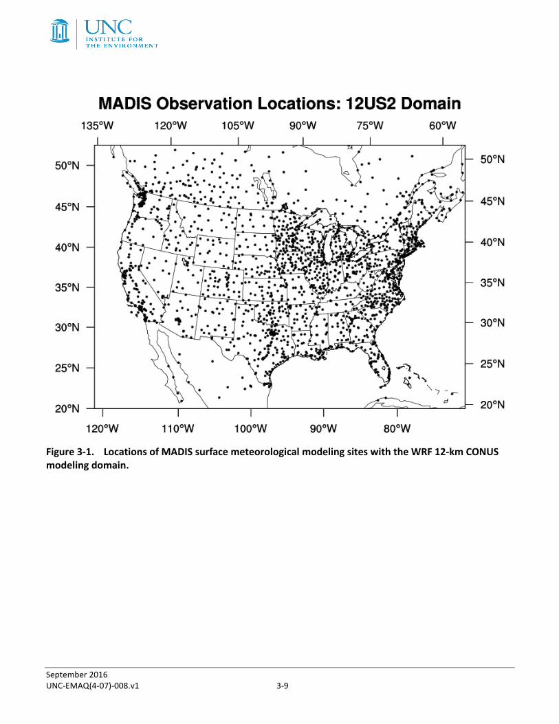
3.0 MODEL PERFORMANCE EVALUATION APPROACH The model evaluation approach was based on a combination of qualitative and quantitative analyses. The quantitative analysis was divided into monthly summaries of 2-m temperature, 2-m mixing ratio, and 10-m wind speed for each month to help generalize the model bias and error. The observed database for winds, temperature, and water mixing ratio used in this analysis was the National Oceanic and Atmospheric Administration (NOAA) Earth System Research Laboratory (ESRL) Meteorological Assimilation Data Ingest System (MADIS). The locations of the MADIS monitoring sites within the 12-km CONUS are shown in Figure 3-1.

The quantitative model performance evaluation of WRF using surface meteorological measurements was performed using the publicly available AMET evaluation tool.16 AMET calculates statistical performance metrics for bias, error, and correlation for surface winds, temperature, and mixing ratio and can produce time series of predicted and observed meteorological variables and performance statistics. This evaluation only summarizes the meteorological model performance using bias and error model performance statistics metrics with select plots to enhance potential users’ understanding of model performance. However, we provide an online source so data users can independently judge the adequacy of the model simulation. Overall comparisons are offered herein to judge the model efficacy for 2015, but this review does not necessarily cover all potential user needs and applications.

We evaluate the model near surface temperature, mixing ratio (humidity), wind speed, and wind direction bias and error. The equations for bias and error are given below.

Bias = ( )∑=

−N

iii OP

N 1

1

Error = ∑=

−N

iii OP

N 1

1

For the wind direction difference statistics, a difference called wind displacement was applied. Wind displacement is the difference in the U and V vectors of the modeled and observed winds. The displacement is calculated as:

Wind Displacement = abs ((Um – Uo + Vm – Vo ) X (1km/1000m) X (3600s/hr) X 1hr) Where Um and Vm are the U and V components respectively of the modeled wind vector and Uo and Vo are the U and V components of the observed wind vector.

We also evaluated the WRF spatial field of accumulated monthly precipitation against the observed monthly precipitation estimates from the Parameter-elevation Relationships on Independent Slopes Model (PRISM) interpolation procedure. The PRISM interpolation uses approximately 13,000 precipitation measurement sites across the CONUS and interpolates them to a < 1 km grid using

16 AMET evaluation tool; https://www.cmascenter.org/help/documentation.cfm?MODEL=amet&VERSION=1.1&temp_id=99999


regression weights based primarily on the physiographic similarity of stations to the grid cell.17 Factors considered are location, elevation, coastal proximity, topographic facet orientation, vertical atmospheric layer, topographic position, and orographic effectiveness of the terrain. The PRISM interpolation approach represents a significant improvement over other techniques used to spatially interpolate observed precipitation that failed to account for factors that influence precipitation away from the observations, such as orographic effects. However, it is still an interpolation technique that may not always capture all effects on precipitation and is just limited to precipitation within the CONUS. The PRISM interpolation procedure will be particularly challenged during summer convective precipitation events (thunderstorms) that can be very spotty and isolated. Such events can occur between the rainfall monitoring sites, and so would not be present in the observations, and hence, the PRISM analysis fields. In our comparison, we regrid PRISM precipitation estimates to take a difference between WRF and PRISM for each month to help illuminate the WRF precipitation errors.

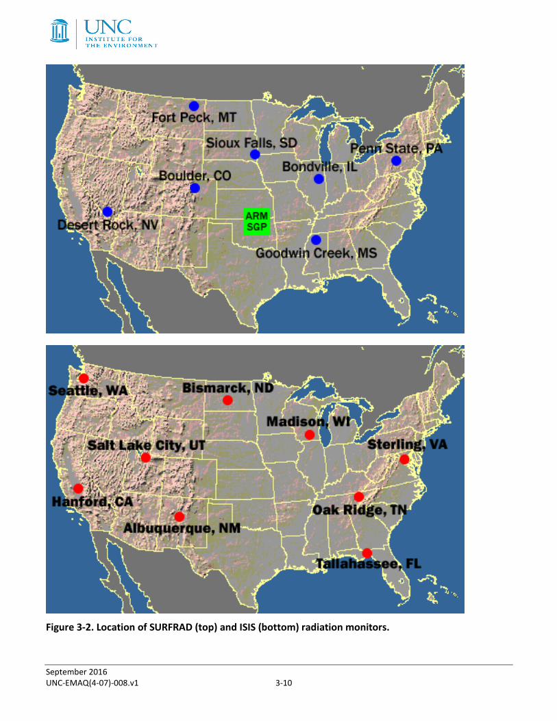
Lastly, model evaluation includes comparison with shortwave downward radiation measurements. Shortwave downward radiation measurements are taken at Surface Radiation Budget Network (SURFRAD)18 and Integrated Surface Irradiance Study (ISIS)19 monitor locations. The SURFRAD network consists of seven sites and the ISIS network consists of nine sites across the United States, shown in Figure 3-2. Both networks are operated by NOAA, with SURFRAD sites existing as a subset of ISIS monitors that provide higher-level radiation information not used in this evaluation.

17 Daley, C., M. Halbleib, J. Smith, W. Gipson, M. Doggett, G. Taylor, J. Curtis and P. Pasteris, 2008. Physiographically sensitive mapping of the climatological temperature and precipitation across the conterminous United States. International. Journal of Climatology, Volume 28, pp 2031-2064. 18 http://www.srrb.noaa.gov/surfrad 19 http://www.esrl.noaa.gov/gmd/grad/isis/index.html

http://www.srrb.noaa.gov/surfrad


Figure 3-1. Locations of MADIS surface meteorological modeling sites with the WRF 12-km CONUS modeling domain.


Figure 3-2. Location of SURFRAD (top) and ISIS (bottom) radiation monitors.


4.0 WRF MODEL PERFORMANCE EVALATUION RESULTS

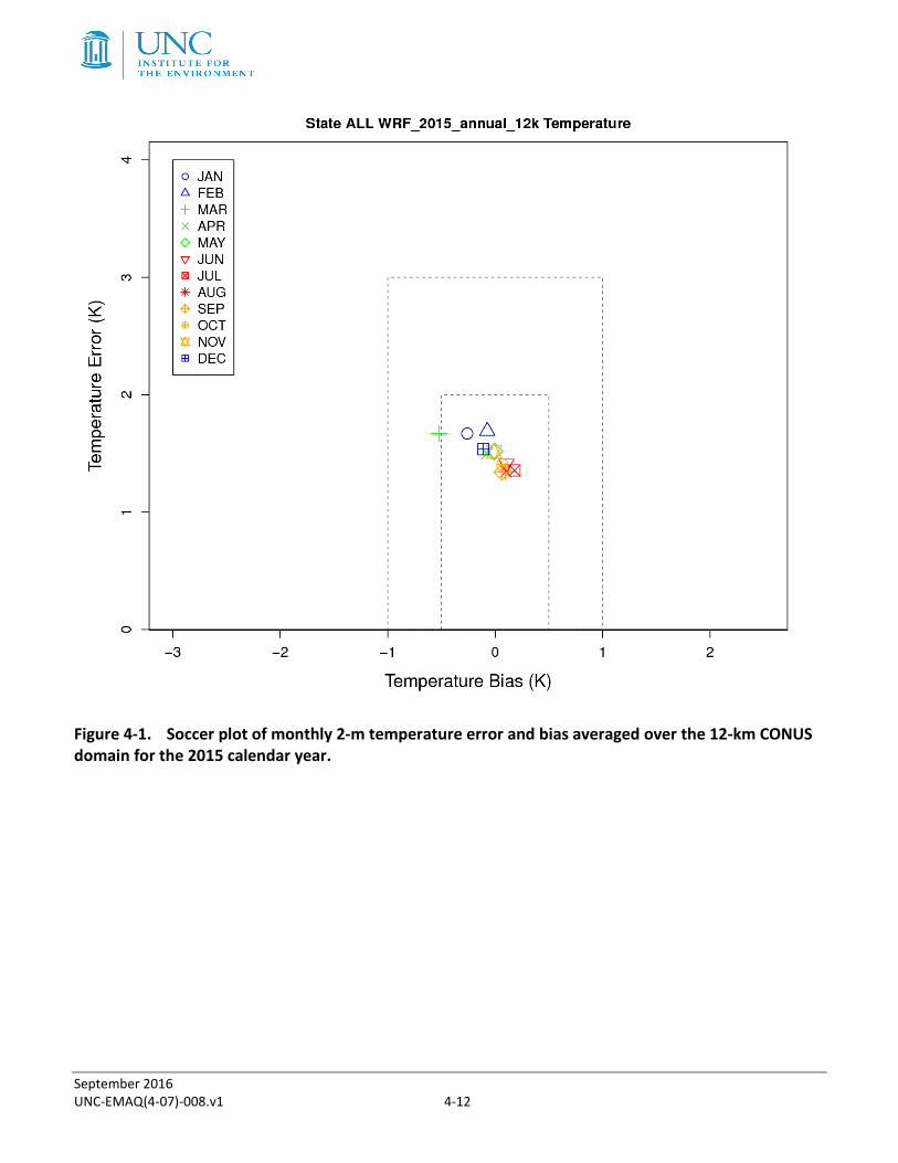
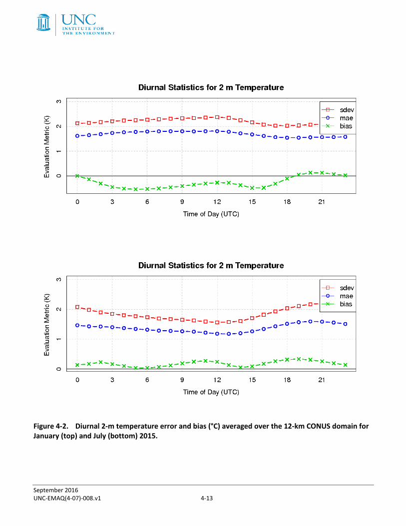
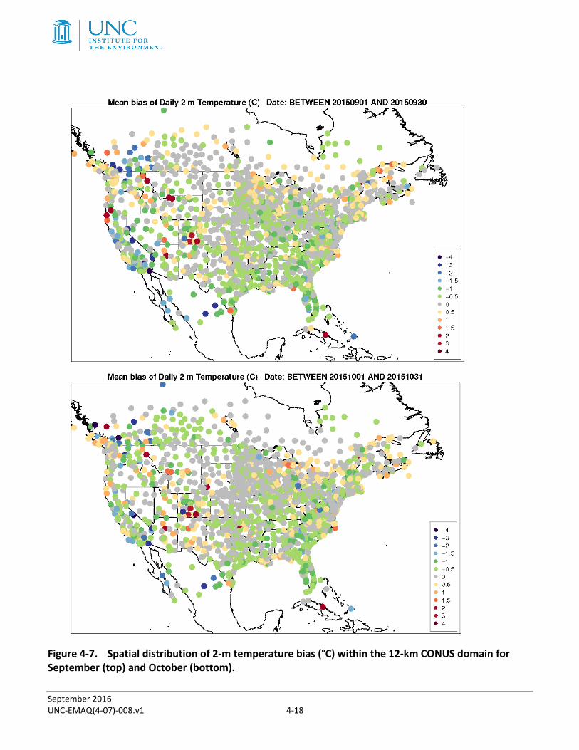
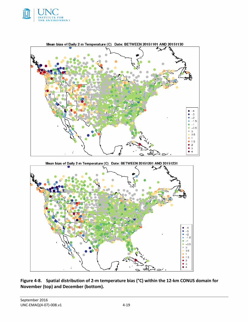
Model Evaluation Results for 2-m Temperature The temperature bias and error on average for the CONUS are shown in Figure 4-1. On average, there is a warm bias during the summer and fall months and a cool bias during the winter and spring months. The bias is smaller than ±1K for all months, excluding March. The temperature errors for all months are between 1K and 2K. Figure 4-2 shows the diurnal temperature statistics for January and July. The diurnal plot illustrates a cool bias in January (winter) that exists throughout the day; however, the bias is largest during the night and early morning and improves during the afternoon hours. The error during January (winter) is also largest during the night and early morning. The opposite is true for July (summer), with a general warm bias throughout the day. The bias and error for July (summer) is largest during the afternoon/evening hours and smallest overnight into the early morning hours. Figure 4-3 illustrates a cool bias of approximately -1°C during January for the eastern half of the CONUS (Great Plains and eastward). However, some portions of the western CONUS (Rocky Mountains and westward) have a warm bias during January. As for February, many locations throughout the Great Plains switch to a warm bias of approximately 0.5°C, but locations such as those over the Northeast U.S. remain cooler than observed. During March and April, shown in Figure 4-4, there remains a cool bias that is largest in the Northeast U.S., upwards of -2°C during March. For the western half of the CONUS, most locations illustrate a cool bias that is typically larger in March compared to April. Figure 4-5 and Figure 4-6 depict the model temperature bias from late spring into the early summer. For many locations throughout the CONUS, there is a clear transition from a cool bias to a warm bias by late summer (August). However, there are also some notable persistent cool bias along the Gulf coast of Texas, southern California, and some locations along the Appalachian Mountains. By late fall and early winter, Figure 4-7 and Figure 4-8, there is a transition back to a cool bias for many locations throughout the eastern half of the CONUS, especially within the Southeast U.S. However, a warm bias during early fall, September/October, persists for locations over the Great Lakes and Northeast U.S. A warm bias is also found during September and October for coastal locations within the Pacific Northwest with a cool bias over central and southern California. In all seasons, stations within the intermountain West have some of the largest biases, upwards of ±4°C.


Figure 4-1. Soccer plot of monthly 2-m temperature error and bias averaged over the 12-km CONUS domain for the 2015 calendar year.


Figure 4-2. Diurnal 2-m temperature error and bias (°C) averaged over the 12-km CONUS domain for January (top) and July (bottom) 2015.


Figure 4-3. Spatial distribution of 2-m temperature bias (°C) within the 12-km CONUS domain for January (top) and February (bottom).


Figure 4-4. Spatial distribution of 2-m temperature bias (°C) within the 12-km CONUS domain for March (top) and April (bottom).


Figure 4-5. Spatial distribution of 2-m temperature bias (°C) within the 12-km CONUS domain for May (top) and June (bottom).


Figure 4-6. Spatial distribution of 2-m temperature bias (°C) within the 12-km CONUS domain for July (top) and August (bottom).


Figure 4-7. Spatial distribution of 2-m temperature bias (°C) within the 12-km CONUS domain for September (top) and October (bottom).


Figure 4-8. Spatial distribution of 2-m temperature bias (°C) within the 12-km CONUS domain for November (top) and December (bottom).


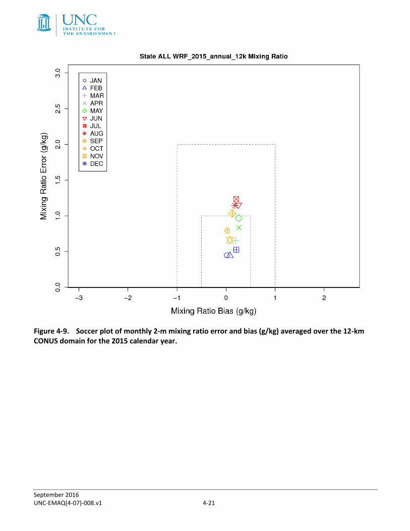
Model Evaluation Results for 2-m Mixing Ratio In general, there is a positive bias for the mixing ratio for the CONUS in 2015, shown in Figure 4-9. The mixing ratio error is largest during the summer months (June, July, August) and smallest during the winter when the moisture capacity of the atmosphere is reduced. Overall, the mixing ratio bias is smaller than ±0.5 g/kg and error less than 1.0 g/kg outside of the warmest months from June - September.

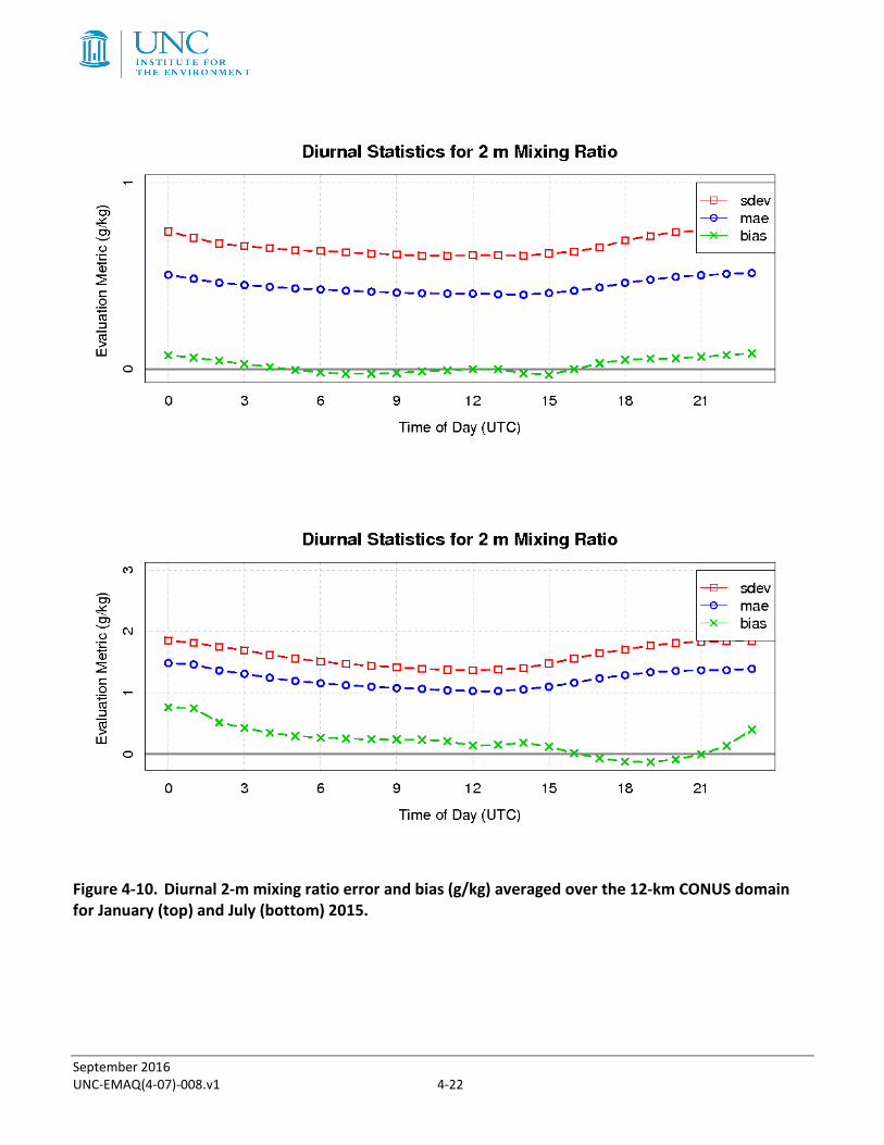
The diurnal statistics of the mixing ratio illustrate differences in the behavior of the mixing ratio bias between January (winter) and July (summer), seen in Figure 4-10. During the winter months, a positive bias is found during the afternoon into the evening. The mixing ratio bias remains neutral for the remainder of the day. The diurnal statistics are different during the summer months, as illustrated by July. A positive mixing ratio bias exists for much of the day and is largest during the evening hours. The bias is near neutral or slightly negative during the afternoon.

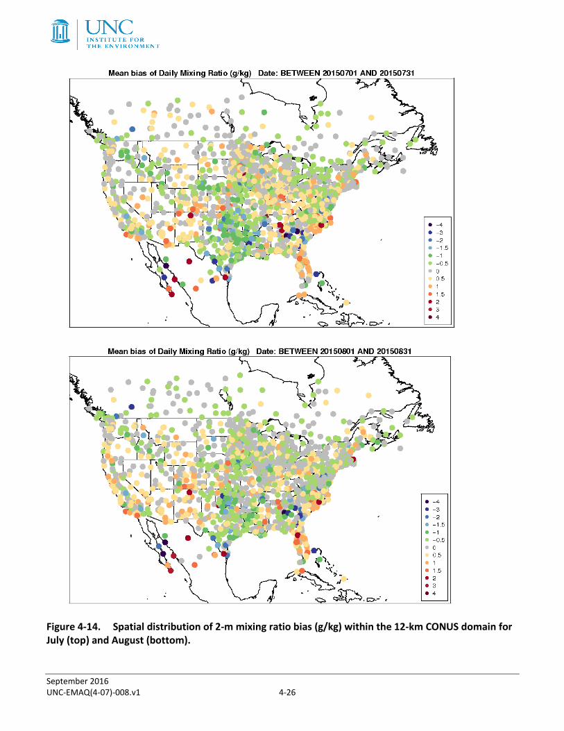
During winter (January and February), many locations throughout the CONUS have a mixing ratio bias smaller than ±0.5 g/kg, seen in Figure 4-11. In particular, a consistent near bias smaller than ±0.5 g/kg is found for stations around the Great Lakes and northeastern US. However, a notable negative bias exists for locations within the central U.S., extending into the southeastern U.S. during the winter months. During the spring months (March and April), shown in Figure 4-12, a noticeable gradient in the bias exists within the eastern half of the U.S. A positive bias (> +0.5 g/kg) extends from Texas into the northeastern U.S. However, a persistent negative bias exists (< -0.5g/kg) for locations just to the west of parts of the Midwest. Over the western half of the CONUS, a persistent negative bias is found within California during the spring months. From late spring (May) throughout the summer (June, July, August), a positive bias emerges for much of the eastern half of the CONUS and for parts of the Southwest U.S., Figure 4-13 and Figure 4-14. The large positive bias for these regions are quickly reduced by October, depicted in Figure 4-15. In November and December, the mixing ratio bias becomes negative for many locations for the eastern half of the CONUS, with a few exceptions for coastal locations along the U.S. East Coast from North Carolina to New England and locations within the Midwest, Figure 4-16.


Figure 4-9. Soccer plot of monthly 2-m mixing ratio error and bias (g/kg) averaged over the 12-km CONUS domain for the 2015 calendar year.


Figure 4-10. Diurnal 2-m mixing ratio error and bias (g/kg) averaged over the 12-km CONUS domain for January (top) and July (bottom) 2015.


Figure 4-11. Spatial distribution of 2-m mixing ratio bias (g/kg) within the 12-km CONUS domain for January (top) and February (bottom).


Figure 4-12. Spatial distribution of 2-m mixing ratio bias (g/kg) within the 12-km CONUS domain for March (top) and April (bottom).


Figure 4-13. Spatial distribution of 2-m mixing ratio bias (g/kg) within the 12-km CONUS domain for May (top) and June (bottom).


Figure 4-14. Spatial distribution of 2-m mixing ratio bias (g/kg) within the 12-km CONUS domain for July (top) and August (bottom).


Figure 4-15. Spatial distribution of 2-m mixing ratio bias (g/kg) within the 12-km CONUS domain for September (top) and October (bottom).


Figure 4-16. Spatial distribution of 2-m mixing ratio bias (g/kg) within the 12-km CONUS domain for November (top) and December (bottom).


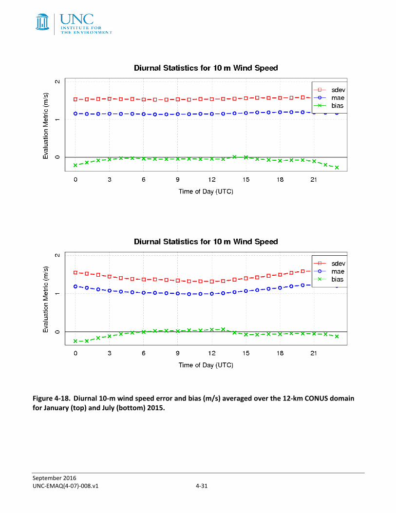
Model Evaluation Results for 10-m Wind Speed All months on average for the CONUS have a wind speed bias smaller than ±0.5 m/s and wind speed error less than 2 m/s, shown in Figure 4-17. Unlike 2-m temperature and mixing ratio, the differences in the bias between winter and summer months are similar, with slightly better performance for wind speed during the summer and early fall.

The diurnal statistics illustrate that the 10-m wind bias is typically larger and negative during the afternoon and evening hours for both January (winter) and July (summer), see Figure 4-18. However, the diurnal bias is smaller than 0.5 m/s. The bias is closer to zero during the night and early morning. There is also a persistent diurnal error, between 1 m/s to 1.5 m/s, for winter and summer months.

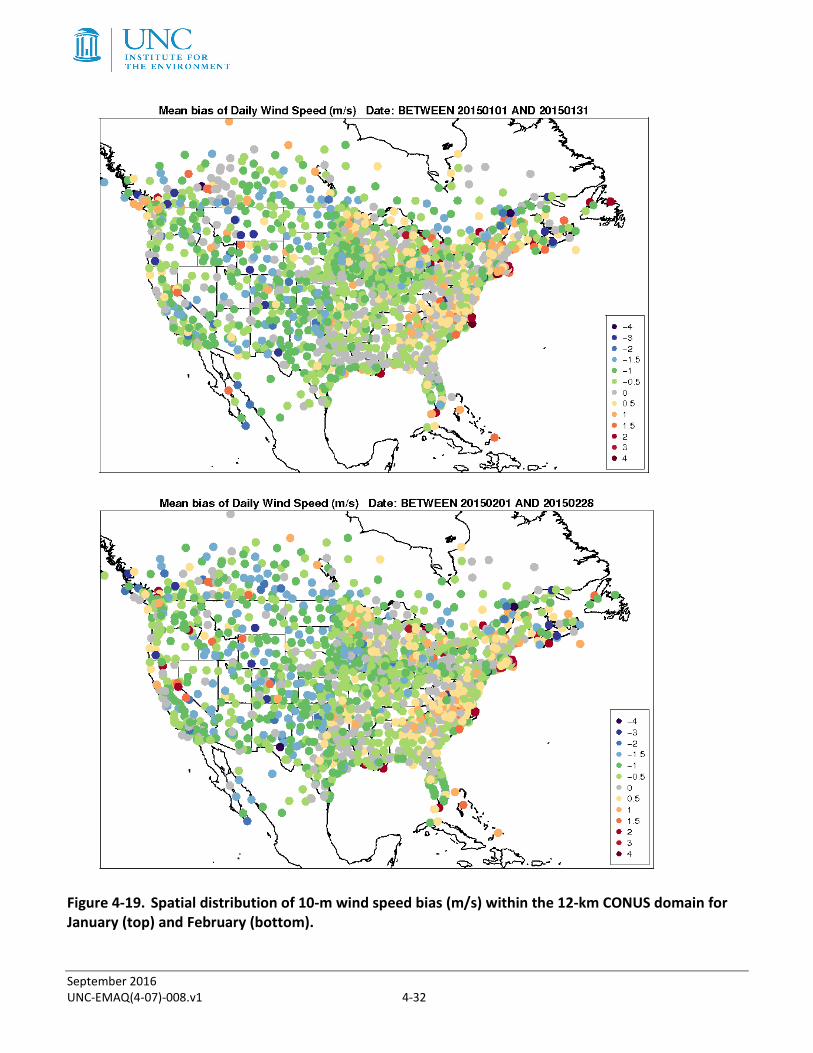
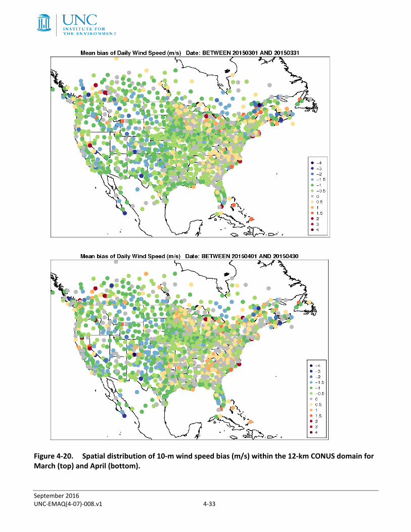
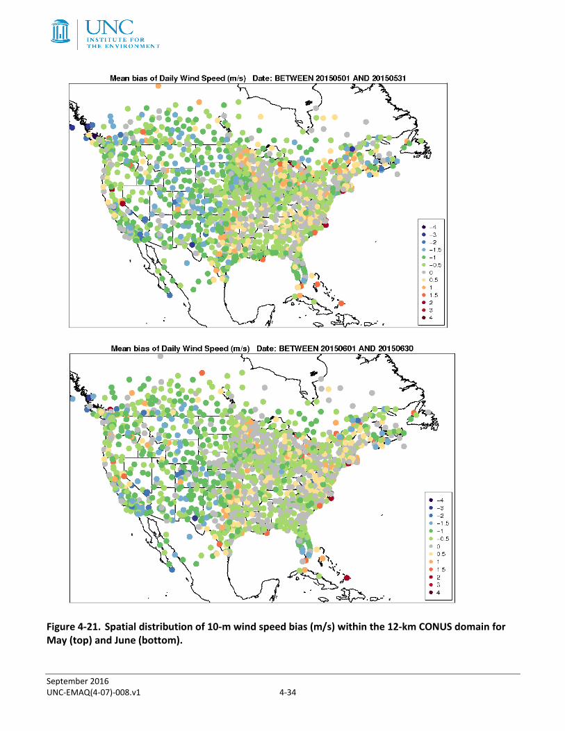
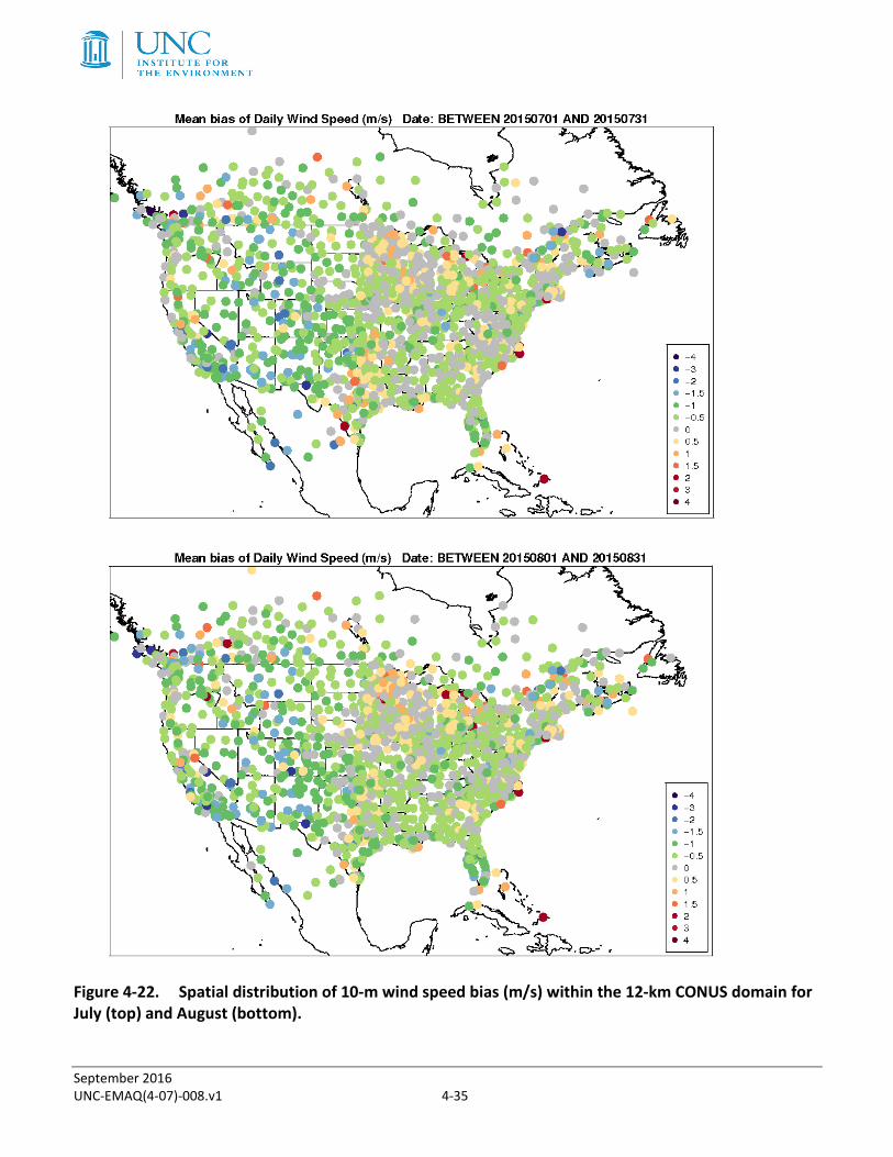
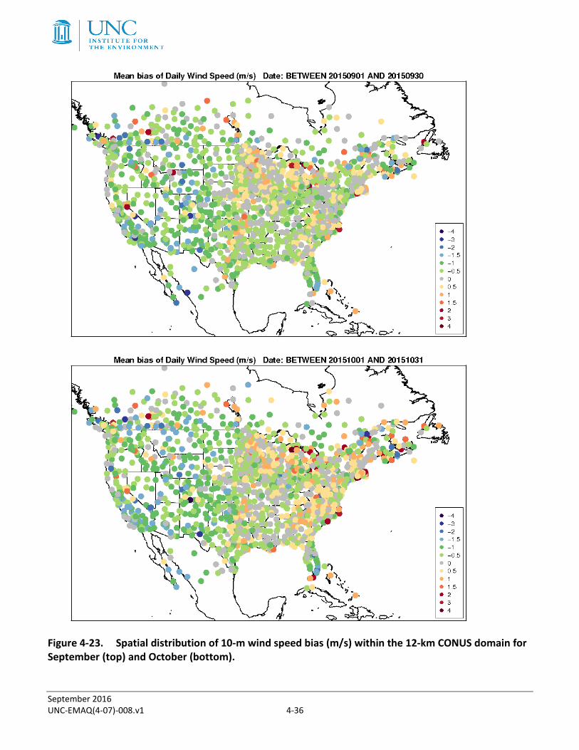
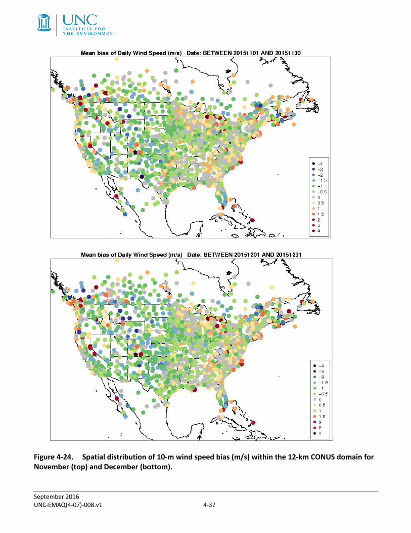
The spatial pattern illustrates the complexity in the wind speed bias throughout the CONUS. During the winter months (January and February), seen in Figure 4-19, the wind speed bias is generally positive for many locations from the Carolinas into the Northeast U.S. and around the Great Lakes. For the remainder of the CONUS, the wind speeds are typically underestimated, with some notable exceptions for the Sierra Nevada and coastal locations within the Pacific Northwest. This pattern continues into the spring months (March, April), Figure 4-20. By summer (June, July, August), Figure 4-21 and Figure 4-22, there are improvements in the wind speed bias for many locations within the CONUS. However, a positive bias occurs for many locations east of the Rockies, with a negative bias from the Rockies, westward. During the fall season into early winter, Figure 4-23 and Figure 4-24, the wind speed bias becomes larger for many locations within the CONUS. Specifically, a positive bias exists for many locations within the eastern half of the CONUS and is largest (exceeding 3-4 m/s) for locations within the Great Lakes region and coastal locations along the East Coast. The western half of the CONUS illustrates the bias is generally negative for many locations with the transition occurring around the western Great Plains. Overall, the largest wind speed biases occur during late fall and into the early winter months with large persistent bias for locations within complex terrain and at land-water interfaces.


Figure 4-17. Soccer plot of monthly 10-m wind speed error and bias (m/s) averaged over the 12-km CONUS domain for the 2015 calendar year.


Figure 4-18. Diurnal 10-m wind speed error and bias (m/s) averaged over the 12-km CONUS domain for January (top) and July (bottom) 2015.


Figure 4-19. Spatial distribution of 10-m wind speed bias (m/s) within the 12-km CONUS domain for January (top) and February (bottom).


Figure 4-20. Spatial distribution of 10-m wind speed bias (m/s) within the 12-km CONUS domain for March (top) and April (bottom).


Figure 4-21. Spatial distribution of 10-m wind speed bias (m/s) within the 12-km CONUS domain for May (top) and June (bottom).


Figure 4-22. Spatial distribution of 10-m wind speed bias (m/s) within the 12-km CONUS domain for July (top) and August (bottom).


Figure 4-23. Spatial distribution of 10-m wind speed bias (m/s) within the 12-km CONUS domain for September (top) and October (bottom).


Figure 4-24. Spatial distribution of 10-m wind speed bias (m/s) within the 12-km CONUS domain for November (top) and December (bottom).


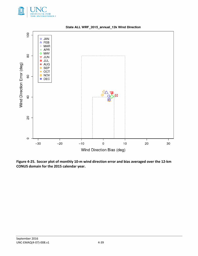
Model Evaluation Results for 10-m Wind Direction The 10-m wind direction error is less than 60 degrees for all months, shown in Figure 4-25. The largest wind direction bias and errors occur during the summer (June, July, August). The best performing months are during the late fall and early winter (October, November, December).

Figure 4-26 illustrates the diurnal statistics for January (winter) and July (summer) and confirms that the average error increases during the summer, by approximately 5 to 10 degrees. However, for both months, the wind direction bias and errors increase overnight and during the early morning hours.

In prior analyses, we illustrated the spatial bias for station locations within the CONUS. For wind direction, we focus on the mean absolute error rather than bias. We focus on the mean absolute error of wind direction because wind direction is a vector field. (Please refer to Section 5 for additional plots including the spatial bias plots of wind direction.) During the winter months (January, February), the mean absolute error is largest for the western states within the CONUS, Figure 4-27. The large errors over the western states within the CONUS are likely a result of the model’s inability to resolve the complex topography and can generally be found for all months. During the winter months, the mean absolute errors are also larger within the Southeast U.S. and eastern Texas, with best performance for locations within the Midwest U.S. The wind direction errors typically improve for locations across the eastern half of the CONUS by April, including the larger errors found during winter within the Southeast U.S. and eastern Texas, Figure 4-28. During the summer (June, July, August), the wind direction errors increase within the Southeast U.S. by as much as 30 degrees, compared to winter and spring, Figure 4-29 and Figure 4-30. The best performing locations during the summer are centered along the climatologically favored region for a strong low-level jet (from Texas into the Midwest). Additionally, during the summer there are notable improvements for some locations for the western half of the CONUS, such as for the Sacramento and San Joaquin Valleys. By the fall season (October, November), the wind direction errors are typically smaller than the summer months for locations within the eastern half of the CONUS, Figure 4-31 and Figure 4-32, but some large errors persist for locations within the Southeast U.S.

Average wind vector displacement (km) for the CONUS domain is shown in Figure 4-33. The top panel illustrates the hourly wind displacement and the bottom panel the monthly wind displacement. The mean wind displacement for both hourly and monthly models is approximately 5-km. The hourly data illustrates that the mean wind vector displacement increases during the afternoon and early evening hours. However, the monthly wind vector displacement is distributed across the year. Overall, the mean wind displacement is around 5-km and smaller than the model horizontal resolution of 12-km; thus, negligible impacts due to wind displacement are expected.


Figure 4-25. Soccer plot of monthly 10-m wind direction error and bias averaged over the 12-km CONUS domain for the 2015 calendar year.


Figure 4-26. Diurnal 10-m wind direction error and bias (m/s) averaged over the 12-km CONUS domain for January (top) and July (bottom) 2015.


Figure 4-27. Spatial distribution of 10-m wind direction mean absolute error within the 12-km CONUS domain for January (top) and February (bottom).


Figure 4-28. Spatial distribution of 10-m wind direction mean absolute error within the 12-km CONUS domain for March (top) and April (bottom).


Figure 4-29. Spatial distribution of 10-m wind direction mean absolute error within the 12-km CONUS domain for May (top) and June (bottom).


Figure 4-30. Spatial distribution of 10-m wind direction mean absolute error within the 12-km CONUS domain for July (top) and August (bottom).


Figure 4-31. Spatial distribution of 10-m wind direction mean absolute error within the 12-km CONUS domain for September (top) and October (bottom).


Figure 4-32. Spatial distribution of 10-m wind direction mean absolute error within the 12-km CONUS domain for November (top) and December (bottom).


Figure 4-33. Distribution of wind displacement averaged for all stations within the 12-km CONUS domain for each hour (top) and month (bottom).


Model Evaluation Results for Monthly Precipitation The PRISM-accumulated monthly precipitation was compared to the WRF 12-km domain precipitation amounts for each month of 2015. The PRISM precipitation was aggregated to the WRF 12-km domain to take a difference in the monthly precipitation totals for each month (WRF minus PRISM). Below is a discussion of the precipitation for each month. Note that PRISM data does not include regions outside of the U.S.

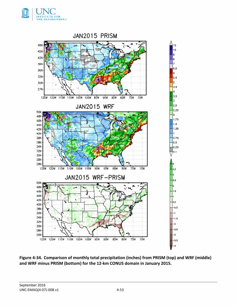
January Precipitation 2015 Figure 4-34 compares the accumulated monthly precipitation from PRISM (top), WRF (middle), and WRF minus PRISM (bottom) for January 2015 within the CONUS. The WRF spatial pattern of monthly precipitation in January 2015 matched the PRISM patterns very well, in areas such as placement of higher rainfall totals for the Pacific Northwest and the eastern half of the CONUS. Climatologically, drier conditions existed for most areas of the U.S. Specifically, areas including California, Nebraska, Oregon, and Wyoming each experienced their top 10 driest January from the 121-year climatological record. No state had a monthly precipitation value ranking among the top 10 wettest on record.20

In examining WRF minus PRISM, the model-accumulated monthly precipitation totals are underestimated (by more than 2 inches) for locations within the coastal Pacific Northwest and states within the Southeast U.S., from Texas into the Carolinas. A notable exception is southern Florida where precipitation is overestimated. Precipitation totals during January are also overestimated for locations within the Northeast U.S., Idaho, and Montana. In general, the overestimated precipitation totals are less than 1 to 2 inches.

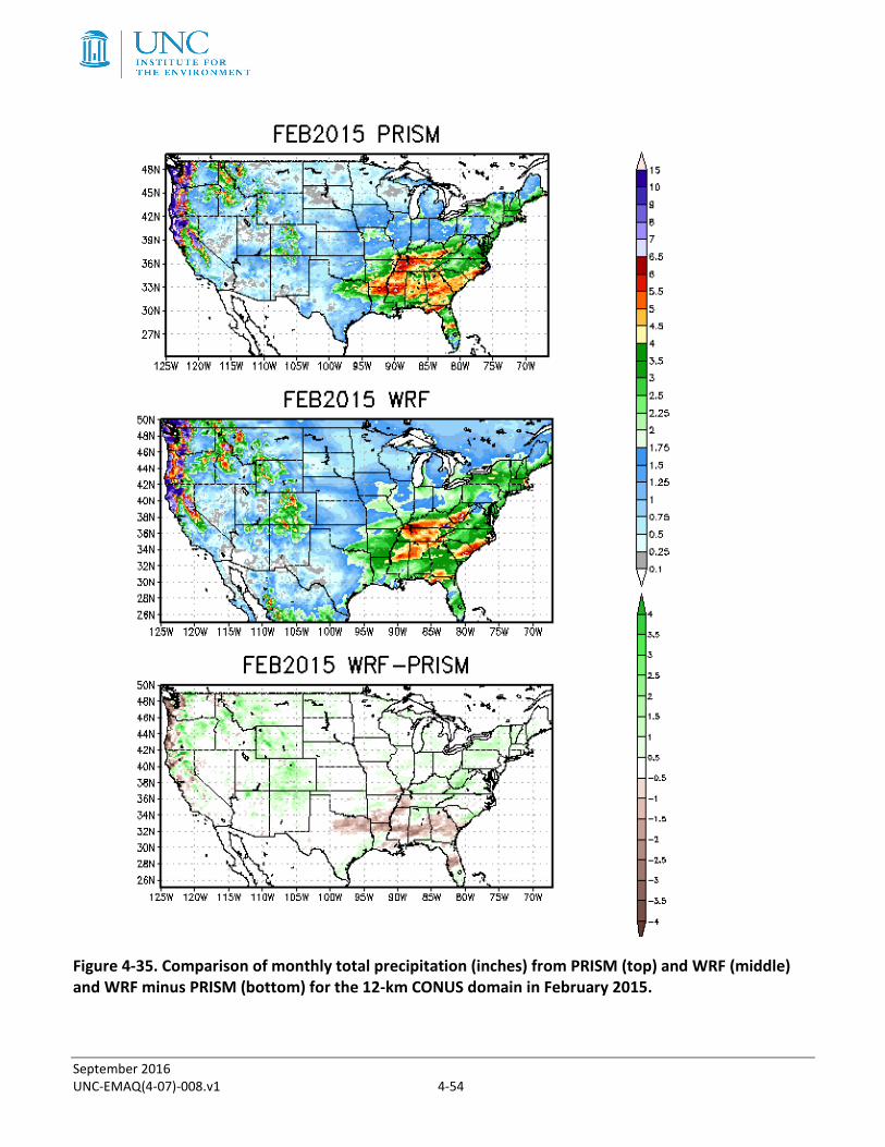
February Precipitation 2015 Figure 4-35 compares the accumulated monthly precipitation from PRISM (top), WRF (middle), and WRF minus PRISM (bottom) for February 2015 within the CONUS. The WRF spatial pattern of monthly precipitation in February 2015 matches the PRISM patterns very well. For instance, WRF simulates higher precipitation totals within the Pacific Northwest and northern California, including the Sierra Nevada. WRF also simulates the heavy rainfall within the Southeast U.S. for locations including Tennessee and the coastal Carolinas. Climatologically, most locations had near to below-average monthly precipitation. No state had February precipitation totals that ranked among the 10 wettest or driest on record.21

In examining WRF minus PRISM, large differences occur in similar locations to the month of January. Underestimation of rainfall occurs for coastal Pacific Northwest and locations within the Southeast U.S., with differences upwards of 3-4 inches. Additionally, rainfall is generally overestimated for the higher terrain locations within the Cascade and Rocky Mountains, especially for Idaho, Wyoming, and Colorado. There is also a noticeable but small overestimation of around one inch for much of the Northeast U.S.

20 https://www.ncdc.noaa.gov/sotc/national/201501 21 https://www.ncdc.noaa.gov/sotc/national/201502


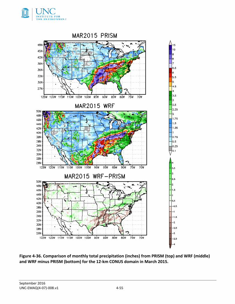
March Precipitation 2015 Figure 4-36 compares the accumulated monthly precipitation from PRISM (top), WRF (middle), and WRF minus PRISM (bottom) for March 2015 within the CONUS. WRF simulates the placement of higher rainfall totals for locations within the CONUS, such as over coastal Texas, Arkansas, Kentucky, West Virginia, and the Cascades. Climatologically, above-average precipitation was observed from the Southern Plains into the Ohio Valley. Specifically, Texas experienced its fourth wettest March on record. Elsewhere, below-average precipitation was observed, with large departures for Nebraska and South Dakota, each having their second driest March on record.22 Overall, WRF is able to simulate the large precipitation gradient that exists within the central U.S.

In examining WRF minus PRISM, WRF provides similar regional bias as in January and February. WRF underestimates precipitation, upwards of 3 to 4 inches, for the coastal locations within the Pacific Northwest and within the Southeast U.S. On the other hand, WRF overestimates the precipitation amounts by 1 to 2 inches for parts of the intermountain West and Northeast U.S.

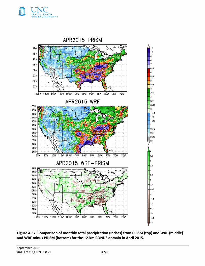
April Precipitation 2015 In April 2015, WRF simulates the correct placement of precipitation for many locations throughout the CONUS, including coastal Texas, Oklahoma, Louisiana, Kentucky, West Virginia, and the Cascade/Sierra Nevada mountain ranges, see Figure 4-37. Wetter than average conditions occurred for Kentucky, Louisiana, and West Virginia. Kentucky experienced its second wettest April on record, with nearly twice the monthly average precipitation. WRF captures the wetter conditions, but does not simulate the heavier precipitation over the southern portion of the state.23 Additionally, there are other locations within the CONUS where WRF fails to simulate heavier precipitation amounts, such as over Georgia.

In examining WRF minus PRISM, WRF underestimates rainfall for parts of the Southeast U.S., particularly from the panhandle of Florida northward to Georgia, Alabama into Tennessee, and southern Kentucky. However, just to the west, WRF overestimates the precipitation for parts of Mississippi and Louisiana and highlights a problem with simulating the exact rainfall placement. As in prior months, WRF overestimates precipitation in the higher elevations over the western half of the CONUS and the Northeast.

May Precipitation 2015 The placement of maximum precipitation in May 2015 was well simulated by WRF with maximum precipitation centered within the central U.S. from Texas to the Dakotas, Figure 4-38. WRF also captures the precipitation gradient towards drier conditions to the east (Alabama/Georgia) and west (New Mexico/Arizona). Climatologically, May 2015 was the wettest May on record for the CONUS, with widespread wetter than average conditions across the central U.S. A total of fifteen states experienced above average precipitation, with Oklahoma and Texas each having their wettest month of any on record, within the last 121 years. WRF does a good job of simulating the placement of precipitation for a significant and record-breaking month. 22 https://www.ncdc.noaa.gov/sotc/national/201503 23 https://www.ncdc.noaa.gov/sotc/national/201504


In examining WRF minus PRISM, WRF underestimates precipitation for areas with some of the heaviest rainfall, including locations within Texas and Oklahoma. However, WRF overestimated the precipitation from the Rockies west towards the Sierra Nevada and underestimated the rainfall east towards the Southeast U.S. Overall, these differences indicate a potential problem in simulating the low-level moisture transport originating from the Gulf of Mexico.

June Precipitation 2015 WRF simulates the large precipitation totals in June 2015 from the Midwest to the Northeast U.S. (from Illinois to Maine), shown in Figure 4-39. Numerous states within these locations had their top 10 wettest June on record.24 Illinois, Indiana, and Ohio each recorded their wettest June of record. WRF is able to simulate the proximity of the record-setting precipitation.

In examining WRF minus PRISM, the WRF precipitation amounts are both over and underestimated for large precipitation totals that extend from the Midwest to the Northeast. Hence, WRF struggles to simulate the precipitation intensity, despite getting the general placement of the rainfall. We also find that WRF overestimates the precipitation totals for southern Texas/Florida and underestimates precipitation totals for eastern Virginia and Louisiana.

July Precipitation 2015 Figure 4-40 compares the accumulated monthly precipitation from PRISM (top), WRF (middle), and WRF minus PRISM (bottom) for July 2015 within the CONUS. WRF simulates the placement of the heaviest precipitation for locations such as New Mexico, Oklahoma, Missouri, Kentucky, and West Virginia. Climatologically, above average precipitation was observed for California, Nevada, New Mexico, and the Ohio Valley. In particular, California and Kentucky experienced their wettest July on record. Locations within California experienced record-breaking precipitation as a result of the remnants of Hurricane Dolores.25 The WRF-simulated precipitation in California is overestimated, particularly in higher elevations of the Sierra Nevada (upwards of 3 to 4 inches), and underestimated for Kentucky (upwards of 3 inches). Additionally, the precipitation associated with the Southwest monsoon is captured in WRF; however, WRF overestimates the amount of rainfall throughout a good portion of the Southwest. For instance, rainfall within Colorado is overestimated by upwards of 4 inches. WRF also overestimates precipitation along the Appalachian Mountains by a similar amount.

August Precipitation 2015 Like July, WRF estimates higher and more widespread precipitation within the Southwest in August 2015 than PRISM, as shown in Figure 4-41. Again, the results illustrate an issue with WRF simulating the North American Monsoon. Like July, the precipitation over the Southwest U.S. is overestimated by WRF and likely the result of an overactive North American Monsoon. However, WRF does an excellent job in simulating some large localized precipitation totals within CONUS, such as over Florida and Iowa. The

24 https://www.ncdc.noaa.gov/sotc/national/201506 25 https://www.ncdc.noaa.gov/sotc/national/201507

https://www.ncdc.noaa.gov/sotc/national/201507


remnants of Tropical Storm Erica helped to contribute to the larger rainfall totals over Florida and parts of Iowa, both of which received twice their normal rainfall during the month of August.26

September Precipitation 2015 In September 2015, there continues to be an overestimation of precipitation from WRF for parts of the Southwest U.S., including Arizona and New Mexico, as shown in Figure 4-42. A percentage of the heavy precipitation in the Southwest was due to the remnants of Hurricane Linda, which caused heavy precipitation in southern California (e.g. Los Angles had its third wettest September).27 Interestingly, the precipitation in southern California is underestimated from WRF, unlike in Arizona and New Mexico. For locations within the Midwest, Mid-Atlantic, Northeast U.S., above average precipitation was observed during September. WRF simulates larger precipitation totals within these regions; however, the precipitation is generally underestimated by several inches. An exception is for the extreme Northeast (e.g. Maine) where WRF overestimates precipitation.

October Precipitation 2015 In October 2015, heavy precipitation returns to the Pacific Northwest and WRF does a good job at capturing the location and the precipitation amounts, shown in Figure 4-43. Above average precipitation was observed for a majority of the southern half of the CONUS, from the Southwest through the Southern Plains and into the Southeast.28 The heaviest precipitation was observed within parts of Texas, Louisiana, and South Carolina. In particular, South Carolina had its second wettest October on record, which is under review because of observed single-day rainfall totals. It is possible after review that October will be the wettest on record for South Carolina. WRF simulates the heavy rainfall for these locations; however, the exact placement of the heaviest rainfall for these locations is slightly different. For instance, WRF simulates heavier precipitation further south within South Carolina than observed within the PRISM dataset.

November Precipitation 2015 In November 2015, WRF simulates heavy precipitation along the Pacific Northwest, seen in Figure 4-44. WRF also simulates the placement of heavier precipitation across the Great Plains, Midwest, and Southeast. WRF underestimates the precipitation totals throughout these regions, especially within the Southeast where WRF underestimates precipitation totals by as much as four inches. Climatologically, the Great Plains, Midwest, and Southeast were much wetter than average, with Arkansas and Missouri having their wettest November on record.29 WRF is unable to simulate the intensity of this climatologically significant event for the central and southern U.S.

26 https://www.ncdc.noaa.gov/sotc/national/201508 27 https://www.ncdc.noaa.gov/sotc/national/201509 28 https://www.ncdc.noaa.gov/sotc/national/201510 29 https://www.ncdc.noaa.gov/sotc/national/201511


December Precipitation 2015 PRISM precipitation for December 2015 was unavailable for this month at the time this report was written and the comparison is not included. Instead, we discuss the WRF precipitation totals for December 2015.

Figure 4-45 is a plot of monthly precipitation totals from WRF for December 2015. WRF illustrates large precipitation totals for the Pacific Northwest, Sierra Nevada, Rockies, and much of the eastern half of the CONUS. WRF precipitation totals exceed 15 inches in the Cascades, Sierra Nevadas, and locations within Oklahoma, Arkansas, and Missouri. December 2015 ranks as the wettest December on average for the CONUS. Twenty-three states had above average precipitation, and Iowa had its wettest December on record.30

30 https://www.ncdc.noaa.gov/sotc/national/201512


Figure 4-34. Comparison of monthly total precipitation (inches) from PRISM (top) and WRF (middle) and WRF minus PRISM (bottom) for the 12-km CONUS domain in January 2015.


Figure 4-35. Comparison of monthly total precipitation (inches) from PRISM (top) and WRF (middle) and WRF minus PRISM (bottom) for the 12-km CONUS domain in February 2015.


Figure 4-36. Comparison of monthly total precipitation (inches) from PRISM (top) and WRF (middle) and WRF minus PRISM (bottom) for the 12-km CONUS domain in March 2015.


Figure 4-37. Comparison of monthly total precipitation (inches) from PRISM (top) and WRF (middle) and WRF minus PRISM (bottom) for the 12-km CONUS domain in April 2015.


Figure 4-38. Comparison of monthly total precipitation (inches) from PRISM (top) and WRF (middle) and WRF minus PRISM (bottom) for the 12-km CONUS domain in May 2015.


Figure 4-39. Comparison of monthly total precipitation (inches) from PRISM (top) and WRF (middle) and WRF minus PRISM (bottom) for the 12-km CONUS domain in June 2015.


Figure 4-40. Comparison of monthly total precipitation (inches) from PRISM (top) and WRF (middle) and WRF minus PRISM (bottom) for the 12-km CONUS domain in July 2015.


Figure 4-41. Comparison of monthly total precipitation (inches) from PRISM (top) and WRF (middle) and WRF minus PRISM (bottom) for the 12-km CONUS domain in August 2015.


Figure 4-42. Comparison of monthly total precipitation (inches) from PRISM (top) and WRF (middle) and WRF minus PRISM (bottom) for the 12-km CONUS domain in September 2015.


Figure 4-43. Comparison of monthly total precipitation (inches) from PRISM (top) and WRF (middle) and WRF minus PRISM (bottom) for the 12-km CONUS domain in October 2015.


Figure 4-44. Comparison of monthly total precipitation (inches) from PRISM (top) and WRF (middle) and WRF minus PRISM (bottom) for the 12-km CONUS domain in November 2015.


Figure 4-45. Monthly total precipitation (inches) from WRF for the 12-km CONUS domain in December 2015.


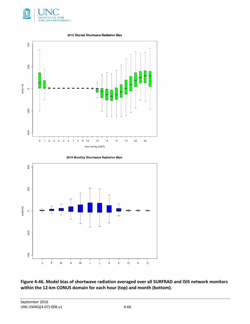
Model Evaluation Results for Solar Radiation Estimates of modeled biogenic emissions for estimating isoprene emissions are sensitive to the photosynthetically activated radiation, which is a fraction of the shortwave downward radiation.31 Regional ozone chemistry and the formation of secondary organic aerosols are impacted by changes in the isoprene emissions. Below, we illustrate the model performance of shortwave downward radiation, which has important implications for regional air quality and provides an indirect assessment of how well the model captures cloud formation during daylight hours.

Figure 4-46 is a comparison of the shortwave downward radiation estimates compared to the surface based measurements at SURFRAD and ISIS network monitors averaged for all sites within the CONUS. The top panel is a comparison of the hourly estimates. The model underestimates the shortwave downward radiation during the early to late morning hours and overestimates the amount during the late afternoon into early evening. The over prediction during the afternoon is larger (upwards +100 W/m2) than the under prediction during the morning hours (-50 W/m2). These results hint at problems simulating the relative cloud cover amount during the morning and afternoon. In the bottom panel is a comparison of the monthly radiation estimates. During the late fall through winter into the early spring, the shortwave radiation bias is small. The bias grows by late spring into the summer, with a peak in the over prediction of shortwave radiation during the months June and July. The over prediction is generally less than 100 W/m2. The median bias is close to zero for all months.

31 Carlton, A.G., Baker. K.R., 2011. Photochemical Modeling of the Ozark Isoprene Volcano: MEGAN, BEIS, and Their Impacts on Air Quality Predictions. Environmental Science and Technology 45, 4438-4445.


Figure 4-46. Model bias of shortwave radiation averaged over all SURFRAD and ISIS network monitors within the 12-km CONUS domain for each hour (top) and month (bottom).


5.0 ADDITIONAL RESULTS An electronic docket is also included with this report that contains additional plots illustrating the 2015 WRF model performance.

Link to additional model evaluation plots for 2015 can be found at:

https://drive.google.com/folderview?id=0BxAQ24gAklsMalhDYllmLWUya1k&usp=sharing

Documents

Weather Research Forecast Version 3.8 Meteorological …WRF is a next-generation mesoscale numerical weather prediction system designed to serve both operational forecasting and atmospheric