Embed Size (px)
Citation preview

WorldMeteorologicalOrganization
Weather. Climate _ Water
Weather Forecasting for
Soaring Flight
Prepared by
Organisation Scientifique et Technique Internationale duVol aVoile (OSTIV)
WMO-No. 1038
2009 edition

WMO-No. 1038
© World Meteorological Organization, 2009
The right of publication in print, electronic and any other form and in any language is reserved byWMO. Short extracts from WMO publications may be reproduced without authorization, providedthat the complete source is clearly indicated. Editorial correspondence and requests to publish, reproduce or translate this publication in part or in whole should be addressed to:
Chairperson, Publications BoardWorld Meteorological Organization (WMO)7 his, avenue de la PaixP.O. Box 2300CH-1211 Geneva 2, Switzerland
ISBN 978-92-63-11038-1
Tel.: +41 (0) 22 7308403Fax: +41 (0) 22 730 80 40E-mail: [email protected]
NOTE
The designations employed in WMO publications and the presentation of material in this publication do notimply the expression of any opinion whatsoever on the part of the Secretariat of WMO concerning the legalstatus of any country, territory, city or area, or of its authorities, or concerning the delimitation of its frontiersor boundaries.
Opinions expressed in WMO publications are those of the authors and do not necessarily reflect those of WMO.The mention of specific companies or products does not imply that they are endorsed or recommended by WMOin preference to others of a similar nature which are not mentioned or advertised.

CONTENTS
Page
FOREWORD....................................................................................................................................... v
INTRODUCTION vii
CHAPTER 1. ATMOSPHERIC PROCESSES ENABLING SOARING FLIGHT...................................... 1-1
1.1 Overview.................................................................................................................................. 1-1
1.2 Convective lift 1-21.2.1 Introduction........................................................................................... 1-21.2.2 Thermal size and strength 1-21.2.3 Distribution and life cycle of thermals 1-31.2.4 Diurnal variation of thermals...................................................................................... 1-31.2.5 Factors influencing thermals....................................................................................... 1-51.2.6 Organized convection 1-91.2.7 A pilot's view: a flight in thermal lift 1-9
1.3 Ridge lift................................................................................................................................... 1-10
1.3.1 Mechanism 1-101.3.2 Meteorological factors 1-11
1.4 Wave lift................................................................................................................................... 1-12
1.4.1 Waves in the atmosphere: wind and stability............................................................. 1-121.4.2 Idealized two-dimensional mountain-wave system.................................................... 1-131.4.3 Variations from the idealized conceptual model........................................................ 1-141.4.4 A pilot's view: a flight in wave lift............................................................................... 1-18
1.5 Combined lift and other lift sources 1-19
1.5.1 Convective waves 1-191.5.2 Other possibilities........................................................................................................ 1-191.5.3 A pilot's view: a flight in combined lift....................................................................... 1-19
1.6 Hazards 1-21
1.6.1 Thunderstorms 1-211.6.2 Strong winds and wind shear...................................................................................... 1-22
CHAPTER 2. GLIDERS AND SOARING FLIGHT 2-1
2.1 Classes and performance......................................................................................................... 2-1
2.1.1 Straight-flight performance........................................................................................ 2-22.1.2 Climb performance 2-2
2.2 Cruising speed 2-3
2.2.1 Localized lift 2-32.2.2 Extended lift 2-4
2.3 Ground speed........................................................................................................................... 2-4
2.4 Effects on performance............................................................................................................ 2-4
2.5 Instrumentation and equipment............................................................................................. 2-4
2.6 Procedures and operations................................................................................. 2-5
2.6.1 Ground handling......................................................................................................... 2-52.6.2 Take-off 2-52.6.3 Flight............................................................................................................................ 2-62.6.4 Final glide and landing 2-6
2.7 Types of flight......................................................... 2-6
2.7.1 Instructional and local flights 2-6

iv
2.7.22.7.32.7.4
CONTENTS
Cross-country flights .Competition flights .Record flights .
Page2-62-62-7
CHAPTER 3. WEATHER FORECASTS................................................................................................ 3-1
3.1 Observations and measurements............................................................................................. 3-1
3.2 Numerical weather prediction................................................................................................. 3-1
3.2.1 General........................................................................................................................ 3-13.2.2 Data assimilation......................................................................................................... 3-23.2.3 Parameterization.......................................................................................................... 3-23.2.4 Application models 3-53.2.5 Model products............................................................................................................ 3-6
3.3 Soaring forecasts 3-93.3.1 Convective lift........................................................................... 3-123.3.2 Horizontal convective rolls 3-163.3.3 Ridge lift................................................................................. 3-173.3.4 Wave lift 3-17
CHAPTER 4. METEOROLOGICAL SUPPORT FOR SOARING FLIGHT............................................. 4-1
4.1 Self-briefing.............................................................................................................................. 4-1
4.2 Personal briefing 4-1
4.2.1 Meteorological support for competitions 4-14.2.2 Preparation of soaring forecasts 4-14.2.3 Meteorological support for the task-setter 4-34.2.4 Documentation for pilots............................................................................................ 4-44.2.5 Competition briefing................................................................................................... 4-44.2.6 Monitoring the weather 4-54.2.7 Pilot support... 4-5
4.3 Meteorological flight planning................................................................................................ 4-5
CHAPTER 5. FLIGHT DATA............................................................................................................... 5-1
5.1 Flight documentation.............................................................................................................. 5-15.1.1 Flight recorder 5-15.1.2 Flight data analysis...................................................................................................... 5-15.1.3 Flight data sources....................................................................................................... 5-1
5.2 Position of updraughts 5-1
5.2.1 Thermal lift.................................................................................. 5-15.2.2 Ridge lift 5-25.2.3 Wave lift 5-2
5.3 Statistical analysis 5-2
5.3.1 Recorded climb rate..................................................................................................... 5-45.3.2 Recorded altitude......................................................................................................... 5-45.3.3 Convective boundary layer depth and climb rate 5-4
5.4 Verification of soaring forecasts............................................................................................... 5-6
5.4.1 Thermal lift.......................................................................... 5-65.4.2 Wave lift 5-7
CHAPTER 6. EPILOGUE 6-1
CHAPTER 7. REFERENCES 7-1
7.1 Articles 7-1
7.2 Bibliography............................................................................................................................. 7-2
7.3 Websites 7-2
APPENDIX A-I
FOREWORD
The key importance of soaring flight skills wasrecently highlighted in the media through thesuccessful emergency "landing" over the HudsonRiver of an airliner which had fully lost its power. Itis remarkable that the pilot involved in this emergency was also an experienced glider pilot, therebyunderscoring the potential benefits of extendingthese skills to aviation as a whole.
The second edition of WMO Technical NoteNo. 158 Handbook of Meteorological Forecasting forSoaring Flight was released in 1993 as WMO-No. 495.From that time, significant changes have occurredin soaring flight forecasting, in particular sinceNumerical Weather Prediction has considerablyprogressed towards the spatial and temporal resolutions required to generate important physicalvariables needed for non-powered flight, such asclimb rates and their temporal and spatialdistributions.
Data volume from numerical weather predictioncentres to pilots has increased significantly andimproved predicted weather interfaces are nowaccessible to pilots. Available weather informationand forecasts further support pre-flight decisionmaking and, reciprocally, flight recorders arecontributing quantitatively to predictionimprovement.
Accordingly, the International Scientific andTechnical Soaring Organisation (OSTlV Organisation Scientifique et TechniqueInternationale du Vol aVoile) meteorological panel,under the chairmanship of Mr Hermann Trimmel,took the initiative to produce this update in orderto document progress achieved.
The following experts have contributed theirknowledge, experience and time to this publication: Rene Heise (Germany), Wolf-Dietrich Herold
(Argentina), Rolf Hertenstein (United States),Edward Hindman (United States), Olivier Liechti(Switzerland), Erland Lorenzen (Germany), ChristofMaul (Germany), Daniel Murer (Switzerland), BedaSigrist (Switzerland) and Hermann Trimmel(Austria). To make the publication truly international, the follOWing experts served as reviewers:Zafer AsIan (Turkey), Tom Bradbury (UnitedKingdom), Dan Gudgel (United States), ]oergHacker (Australia) and Bernt Olofsson (Sweden).
Mr Olivier Liechti has served as working groupchairman and Mr Edward Hindman as editor. TheEuropean Cooperation in Science and Technology(COST) generously provided support to workinggroup sessions and the NMSs of Germany andSwitzerland kindly hosted the meetings. The finaldocument has been reviewed by the WMOCommission for Aeronautical Meteorology (CAeM).
The aim of this Technical Note is to provide thereader an internationally agreed set of guidelinesfor meteorological forecasting in soaring flight andrelated activities. As pointed out in the Introduction,this includes forecasters at busy aerodrome meteorological offices routinely receiving enquiries frompilots, as well as those detached on the field toproVide forecasting support during contests andshows.
WMO is therefore pleased to make this highly relevant publication available to the wider soaringflight community.
. ]arraud)Secretary-General

INTRODUCTION
This publication has been prepared for everyonewho is concerned with the meteorological supportfor gliding. This incl udes designers of pilot selfbriefing systems and those who provide forecastsfor pilots, as ,·vell as contest briefings. The publication is designed to help meteorological forecastersand pilot briefers respond to the requirements ofglider flight operations.
A phenomenological description of atmosphericprocesses relevant to soaring presents the meteorological background for gliding activities. Convectionis by large the most frequently used source of lift forgliders. The dynamical sources of lift are lessfrequent. They do, however, provide the opportunities for extremely fast and long flights. Soaring flightis occasionally limited by meteorological hazards.
A technical description of gliding and soaring flightis presented so that the impact of weather on feasibility, timing, range of operations and safety insoaring may be appreciated.
The classical forecasting framework of routine analysis and interpretation of prognostic charts must beextended to the smaller-scale features relevant tosoaring. More and more numerical analysis andforecasting techniques that address these featuresare appearing. Soaring forecasts for both thermal
and dynamic lift require a certain spatial andtemporal resolution in order to be useful for meteorological flight planning. This publicationaddresses those issues.
The presentation of high-resolution weather forecasts to pilots is a challenging task. It is supportedby new concepts, personal computers and theInternet. Sophisticated self-briefing systems havebeen developed: pilots may use high-resolutionsoaring forecasts for establishing flight plans forindividual tasks. Personal briefings, however, arestill appreciated by task-setters and pilots at soaringcompetitions. Preflight decision-making issupported by high-resolution forecasts and by themonitoring of weather observations in almost realtime.
Finally, recorded flight data are presented thatreveal the flight altitudes used, the climb ratesachieved and the position of the updraughts. Thedata support both the development and the qualityof numerical models for the prediction of soaringconditions. The simulation of documented soaringflights with the predicted weather demonstrates theskill of the state-of-the-art techniques in numericalweather prediction. Such simulations contributequantitatively to the improvement of the numerical models.

CHAPTER 1
ATMOSPHERIC PROCESSES ENABLING SOARING FLIGHT
Whenever a glider deviates from a descending flightgoverned by the aerodynamic characteristics inherent in its design, atmospheric processes are at work.As it is the goal of glider pilots to use these processes to prolong the flight time and to increase thealtitude or distance flown, it seems appropriate tobegin this note with a description of the atmospheric processes relevant to soaring flight, whichare the processes that produce rising and sinkingair, or updraughts and downdraughts.
Note: In this publication rising air can take thenames updraught, updraught rate, lift, climb, climbrate and lift rate. Typically, the rates refer to thespeed a glider is moving away from the Earth'ssurface or the reading from the on-board verticalspeed instrument (called the variometer). Theother terms refer to the speed at which the air isrising. But a glider is always falling through the airdue to its weight. Thus, in the case of rising air, the
variometer reading is always slightly lower than theactual vertical air speed.
1.1 OVERVIEW
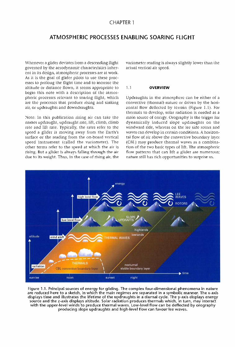
Updraughts in the atmosphere can be either of aconvective (thermal) nature or driven by the horizontal flow deflected by terrain (Figure 1.1). Forthermals to develop, solar radiation is needed as amain source of energy. Orography is the trigger fordynamically induced slope updraughts on thewindward side, whereas on the lee side rotors andwaves can develop in certain conditions. A horizontal flow of air above the convective boundary layer(eBL) may produce thermal waves as a combination of the two basic types of lift. The atmosphericflow patterns that can lift a glider are numerous;nature still has rich opportunities to surprise us.
Figure 1.1. Principal sources of energy for gliding. The complex four-dimensional phenomena in natureare reduced here to a sketch, in which the main regimes are separated in a symbolic manner. The x-axisdisplays time and illustrates the lifetime of the updraughts in a diurnal cycle. The y-axis displays energysource and the z-axis displays altitude. Solar radiation produces thermals which, in turn, may interactwith the upper-level winds to produce thermal waves. Low-level flow can be deflected by orography
producing slope updraughts and high-level flow can favour lee waves.
1-2 WEATHER FORECASTING FOR SOARING FLIGHT
Nowadays, thermals are the most common typeof lift used for cross-country flights. For recordflights, however, dynamic lift aligned in waves, inrotors and along ridges is much morefavourable.
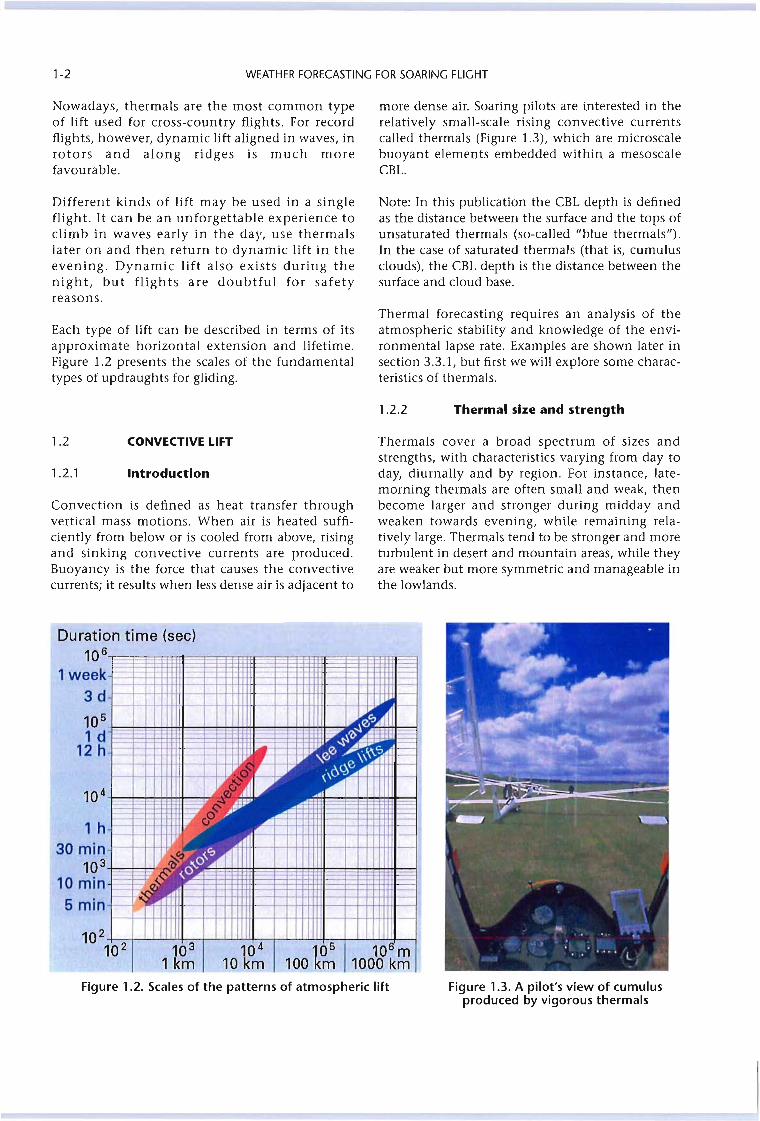
more dense air. Soaring pilots are interested in therelatively small-scale rising convective currentscalled thermals (Figure 1.3), which are microscalebuoyant elements embedded within a mesoscaleCBL.
Different kinds of lift may be used in a singleflight. It can be an unforgettable experience toclimb in waves early in the day, use thermalslater on and then return to dynamic lift in theevening. Dynamic lift also exists during thenight, but flights are doubtful for safetyreasons.
Note: In this publication the CBL depth is definedas the distance between the surface and the tops ofunsaturated thermals (so-called "blue thermals").In the case of saturated thermals (that is, cumulusclouds), the CBL depth is the distance between thesurface and cloud base.
Each type of lift can be described in terms of itsapproximate horizontal extension and lifetime.Figure 1.2 presents the scales of the fundamentaltypes of updraughts for gliding.
Thermal forecasting requires an analysis of theatmospheric stability and knowledge of the environmental lapse rate. Examples are shown later insection 3.3.1, but first we will explore some characteristics of thermals.
1.2.2 Thermal size and strength
1.2 CONVECTIVE LIFT
1.2.1 Introduction
Convection is defined as heat transfer throughvertical mass motions. When air is heated sufficiently from below or is cooled from above, risingand sinking convective currents are produced.Buoyancy is the force that causes the convectivecurrents; it results when less dense air is adjacent to
Thermals cover a broad spectrum of sizes andstrengths, with characteristics varying from day today, diurnally and by region. For instance, latemorning thermals are often small and weak, thenbecome larger and stronger during midday andweaken towards evening, while remaining relatively large. Thermals tend to be stronger and moreturbulent in desert and mountain areas, while theyare weaker but more symmetric and manageable inthe lowlands.
Duration time (sec)
106~~11~11~~11~1~1 weeki=3 d J-t-++-tt1rtt1---+-++-If-tttHI---j----f---H-H-ttI--t-++++
105~iI~.Ii.11 d12 h
104m.~1 h t-t-++++I-ti'I
30 minJ---t-f-HV
103~§~~!1131110 min~: ~
5 min
Figure 1.2. Scales of the patterns of atmospheric lift Figure 1.3. A pilot's view of cumulusproduced by vigorous thermals
CHAPTER 1. ATMOSPHERIC PROCESSES ENABLING SOARING FLIGHT 1-3
Visual indicators of thermals include dust devils,haze domes (pre-cumulus clouds), cumulus clouds,as well as circling birds or gliders, all of which indicate a limited size. Individual thermal updraughtsdo not encompass broad areas as do other updraughttypes (for example, mountain lee waves). Turbulenteddies of many sizes constitute the CBL; thermalsform a subset of these.
A typical thermal cross-section diameter is on theorder of 150 to 300 metres, although individualspecimens vary considerably from the norm.Fortunately for soaring pilots, the radius of turn ofa circling glider falls into this range. A glider at atrue airspeed of 98 km/h (50 knots) with a 40° bankangle flies a circle with a diameter of about 170metres (550 feet). Thermals can be \,veak enough tobe of little or no use to soaring pilots.
The strength of thermals depends on the air masscharacteristics, the landscape and available insolation. Average thermal conditions vary from regionto region. A low-lying soaring site at high latitudesmight normally find thermals in the range of 1 to 2metres per second (m/s), while thermals of 4 or 5m/s would be rare. By contrast, at a desert Site,5 m/s thermals are common during summermonths. In a given thermal-soaring season (springthrough fall), every thermal-soaring site experiences days on which thermal strength is weak, andother days on which thermals are strong.
Thermal height and strength tend to be correlated.The higher thermals go, the stronger they are. Thestrongest thermal updraughts occur at a heightabout midway through the CBL and decrease in theupper third of the CBL.
Days with cumulus have relatively more moisturein the air. Moist air is more buoyant than dry air;hence, days with cumulus tend to have strongerthermals.
1.2.3 Distribution and life cycle ofthermals
Field studies have shown that when CBLs arebetween 600 and 1 200 metres deep, the ratio ofthermal spacing to CBL depth is about 1.5. On dayswith deep CBLs (1 800 to 3 000 metres aboveground level, or AGL), the ratio increases to 5 or 10,and sometimes greater. As a general rule, the deeperthe CBL, the greater the spacing between thermals.
Once away from the strong sinking air at the edgeof thermals, the CBL is characterized by broad areasof weak downdraughts. Evenly spaced thermals
typically occur over relatively uniform flat terrain,and in fairly light winds. Thermal and sink distributions may be highly variable, and sometimes largeareas are void of thermals. Sought-after organizedlines of lift can also form, however. Here we brieflylist several factors that can modify thermaldistribution:(a) Surface features (terrain characteristics, moist
soils, lakes);(b) Extensive cloud cover from overdevelopment
(such as merging or deepening of cumulus),fronts or thunderstorms;
(c) Ridges or mountains (especially under Windyconditions) and mountain lee waves;
(d) Lines or zones of converging air (such as seabreezes) and cloud streets.
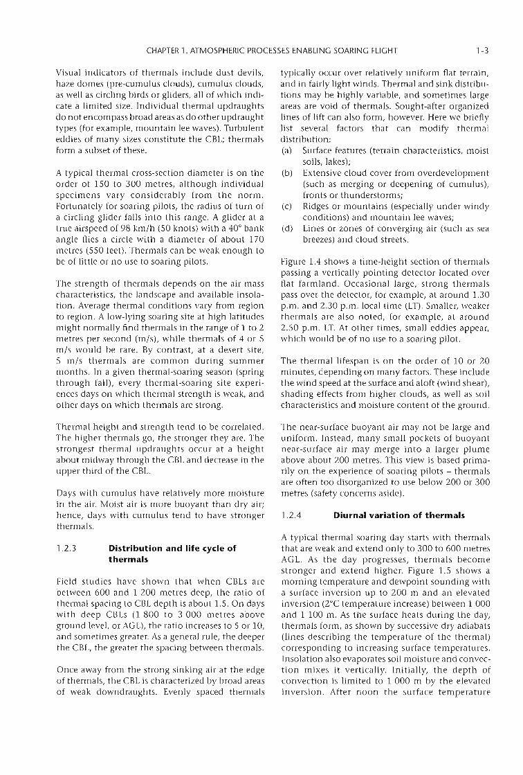
Figure 1.4 shows a time-height section of thermalspassing a vertically pointing detector located overflat farmland. Occasional large, strong thermalspass over the detector, for example, at around 1.30p.m. and 2.30 p.m. local time (LT). Smaller, weakerthermals are also noted, for example, at around2.50 p.m. LT. At other times, small eddies appear,which would be of no use to a soaring pilot.
The thermal lifespan is on the order of 10 or 20minutes, depending on many factors. These includethe wind speed at the surface and aloft (wind shear),shading effects from higher clouds, as well as soilcharacteristics and moisture content of the ground.
The near-surface buoyant air may not be large anduniform. Instead, many small pockets of buoyantnear-surface air may merge into a larger plumeabove about 200 metres. This view is based primarily on the experience of soaring pilots - thermalsare often too disorganized to use below 200 or 300metres (safety concerns aside).
1.2.4 Diurnal variation of thermals
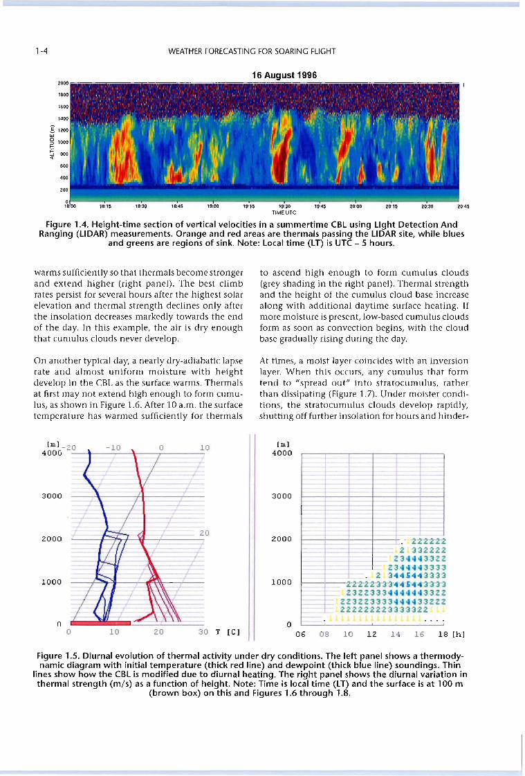
A typical thermal soaring day starts with thermalsthat are weak and extend only to 300 to 600 metresAGL. As the day progresses, thermals becomestronger and extend higher. Figure 1.5 shows amorning temperature and dewpoint sounding witha surface inversion up to 200 m and an elevatedinversion (2°C temperature increase) between 1 000and 1 100 m. As the surface heats during the day,thermals form, as shown by successive dry adiabats(lines describing the temperature of the thermal)corresponding to increasing surface temperatures.Insolation also evaporates soil moisture and convection mixes it vertically. Initially, the depth ofconvection is limited to 1 000 m by the elevatedinversion. After noon the surface temperature
1-4 WEATHER FORECASTING FOR SOARING FLIGHT
16 August 19962000
1800
1600
1400
I 1200wg 1000...;::-' 800«
600
400
200
18:15 18:30 18:45 19:00 19:15 19:30TIMEUTC
19:45 20:00 20:15 20:30
Figure lA. Height-time section of vertical velocities in a summertime CBL using light Detection AndRanging (lIDAR) measurements. Orange and red areas are thermals passing the lIDAR site, while blues
and greens are regions of sink. Note: Local time (LT) is UTC - 5 hours.
warms sufficiently so that thermals become strongerand extend higher (right panel). The best climbrates persist for several hours after the highest solarelevation and thermal strength declines only afterthe insolation decreases markedly towards the endof the day. In this example, the air is dry enoughthat cumulus clouds never develop.
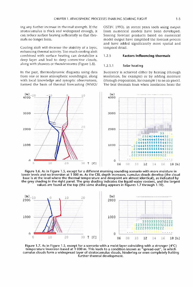
On another typical day, a nearly dry-adiabatic lapserate and almost uniform moisture with heightdevelop in the CBL as the surface warms. Thermalsat first may not extend high enough to form cumulus, as shown in Figure 1.6. After 10 a.m. the surfacetemperature has warmed sufficiently for thermals
[m]400G-2_o_+-_--.-_+_-, ~10
to ascend high enough to form cumulus clouds(grey shading in the right panel). Thermal strengthand the height of the cumulus cloud base increasealong with additional daytime surface heating. Ifmore moisture is present, low-based cumulus cloudsform as soon as convection begins, with the cloudbase gradually rising during the day.
At times, a moist layer coincides with an inversionlayer. When this occurs, any cumulus that formtend to "spread out" into stratocumulus, ratherthan dissipating (Figure 1.7). Under moister conditions, the stratocumulus clouds develop rapidly,shutting off further insolation for hours and hinder-
[m]
4000
20o
06 08 10 12 14 16 18 [hI
3000
2000
1000
no 10
1- =-.::-/"----.;--.
-f-- -!----;--
-r--f-,.-1----r- 20
-f
I-
I t ---~
- f
30 T [Cl
3000
2000
1000
i-:-i===+=-'-j-.' '2'2'2'2'2'22 332222
Z344433ZZZ344443333
2 H4H433331---+---2'2'2'2'2'3'3'3'4'4'1'4'4'3'3'3'3
Z3ZZ33344444433ZZZZ3ZZ3333444433ZZZ222222223333322
Figure 1.5. Diurnal evolution of thermal activity under dry conditions. The left panel shows a thermodynamic diagram with initial temperature (thick red line) and dewpoint (thick blue line) soundings. Thin
lines show how the CBL is modified due to diurnal heating. The right panel shows the diurnal variation inthermal strength (m/s) as a function of height. Note: Time is local time (LT) and the surface is at 100 m
(brown box) on this and Figures 1.6 through 1.8.
CHAPTER 1. ATMOSPHERIC PROCESSES ENABLING SOARING FLIGHT 1-5
OSTIV, 1993). In recent years tools using outputfrom numerical models have been developed.Soaring forecast products based on numericalmodel output have simplified the forecast processand have added significantly more spatial andtemporal detail.
ing any further increase in thermal strength. If thestratocumulus is thick and widespread enough, itcan reduce surface heating sufficiently so that thermals no longer form.
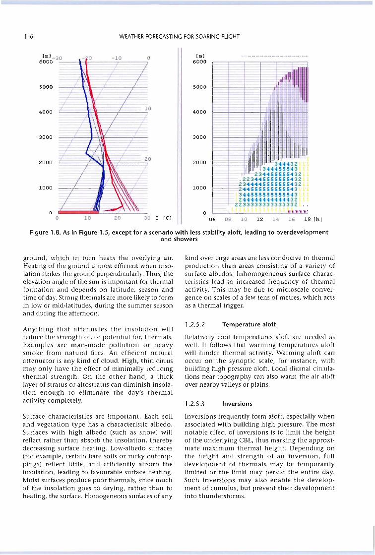
Cooling aloft will decrease the stability of a layer,enhancing thermal activity. Too much cooling aloftcombined with surface heating can destabilize adeep layer and lead to deep convective clouds,along with showers or thunderstorms (Figure 1.8).
1.2.5
1.2.5.1
Factors influencing thermals
Solar heating
In the past, thermodynamic diagrams using datafrom one or more atmospheric sounding(s), alongwith local knowledge and synoptic observations,formed the basis of thermal forecasting (WMO/
Buoyancy is achieved either by heating (throughinsolation, for example) or by adding moisture(through evaporation, for example) to an air parcel.The best thermals form when insolation heats the
[Ill)-20 10 [Ill) ....... ,,,,,, ..,......... " ..... "',,,,,,,,, ...
400G 4000
3000 3000 If
2000 2000 .. 1111 3311232 ... 2 ............ 432324 ......... 44£ ...... 3322244445555555~4332
1000 1000 . '23'4 4 4 5'B 5 B'5'54'3'3 n23 ...... 4 ... £S£££54 ... 3322
223 ... 4 ... 4 ... 4 ...... 44433222.2223333333333322
n 00 10 20 30 T [C) 06 08 10 12 14 16 18 [hI
Figure 1.6. As in Figure 1.5, except for a different morning sounding scenario with more moisture inlower levels and no inversion at 1 000 m. As the CBl depth increases, cumulus clouds develop (the cloudbase is at the level where the thermal temperature and dewpoint are almost identical), as indicated by
the grey shading in the right panel. The grey shading indicates the liquid water content, and the largestvalues are found at the top (the same shading appears in Figures 1.7 through 1.10).
[Ill)200G- l _0__-h_----Ja,--1_0 20
[Ill)
2000"1111'11111111111111111111111111111111111111'"''
o06 08 10 12 14 16 18 [h)
1000
no la 20 30 T [C)
1000 "
t 3333333333ZZ2ZZZ3333333333lZZZZZZZZ333333ZZl
Figure 1.7. As in Figure 1.5, except for a scenario with a moist layer coinciding with a stronger (4°C)temperature inversion based at 1 000 m. This leads to a condition known as "spread-out", in which
cumulus clouds form a widespread layer of stratocumulus clouds, hindering or even completely haltingfurther thermal development.
1-6 WEATHER FORECASTING FOR SOARING FLIGHT
06 08 10 12 14 16 18 (hIo
4000
(ml6000
5000
10
30 T (Cl2010o
(ml600G-3_o__-l-1f,- -_1~0---__,0
4000
n
2000
5000
3000
1000
Figure 1.8. As in Figure 1.5, except for a scenario with less stability aloft, leading to overdevelopmentand showers
ground, which in turn heats the overlying air.Heating of the ground is most efficient when insolation strikes the ground perpendicularly. Thus, theelevation angle of the sun is important for thermalformation and depends on latitude, season andtime of day. Strong thermals are more likely to formin low or mid-latitudes, during the summer seasonand during the afternoon.
kind over large areas are less conducive to thermalproduction than areas consisting of a variety ofsurface albedos. Inhomogeneous surface characteristics lead to increased frequency of thermalactivity. This may be due to microscale convergence on scales of a few tens of metres, which actsas a thermal trigger.
Relatively cool temperatures aloft are needed aswell. It follows that warming temperatures aloftwill hinder thermal activity. Warming aloft canoccur on the synoptic scale, for instance, withbuilding high pressure aloft. Local diurnal circulations near topography can also warm the air aloftover nearby valleys or plains.
Anything that attenuates the insolation willreduce the strength of, or potential for, thermals.Examples are man-made pollution or heavysmoke from natural fires. An efficient naturalattenuator is any kind of cloud. High, thin cirrusmay only have the effect of minimally reducingthermal strength. On the other hand, a thicklayer of stratus or altostratus can diminish insolation enough to eliminate the day's thermalactivity completely.
1.2.5.2
1.2.5.3
Temperature aloft
Inversions
Surface characteristics are important. Each soiland vegetation type has a characteristic albedo.Surfaces with high albedo (such as snow) willreflect rather than absorb the insolation, therebydecreasing surface heating. Low-albedo surfaces(for example, certain bare soils or rocky outcroppings) reflect little, and efficiently absorb theinsolation, leading to favourable surface heating.Moist surfaces produce poor thermals, since muchof the insolation goes to drying, rather than toheating, the surface. Homogeneous surfaces of any
Inversions frequently form aloft, especially whenassociated with building high pressure. The mostnotable effect of inversions is to limit the heightof the underlying CBL, thus marking the approximate maximum thermal height. Depending onthe height and strength of an inversion, fulldevelopment of thermals may be temporarilylimited or the limit may persist the entire day.Such inversions may also enable the development of cumulus, but prevent their developmentinto thunderstorms.
CHAPTER 1. ATMOSPHERIC PROCESSES ENABLING SOARING FLIGHT 1-7
Elevated terrain in mid-latitudes favourablyaffects thermal development in many ways.First, insolation will strike sun-facing slopes at amore-nearly perpendicular angle compared toadjacent valleys or plains. This leads to moreintense heating along sun-facing slopes. Thus,mountains, ridges and even small hills willproduce thermals earlier in the day and later inthe afternoon. On the other hand, valleys andother lowlands are ideal for the formation ofnight-time inversions. After sunset, dense radiatively cooled air sinks down the sides of hills ormountains, pooling in the valleys below. It cantake many hours of heating during the morningbefore cool valley air completely erodes, delaying the onset of thermals over the valley floor.Elevated terrain also drains water, which thencollects in adjacent relatively moist valleys. Thedrier slopes and peaks heat more efficiently,giving stronger thermals and producing themearlier in the day. In contrast, mountainousregions receive more precipitation. This,combined with higher-reaching thermals, meansthat mountainous regions are more likely toproduce cumulus clouds than adjacent lowlands.Elevated terrain is also more likely to producedeep convective clouds and showers, or to
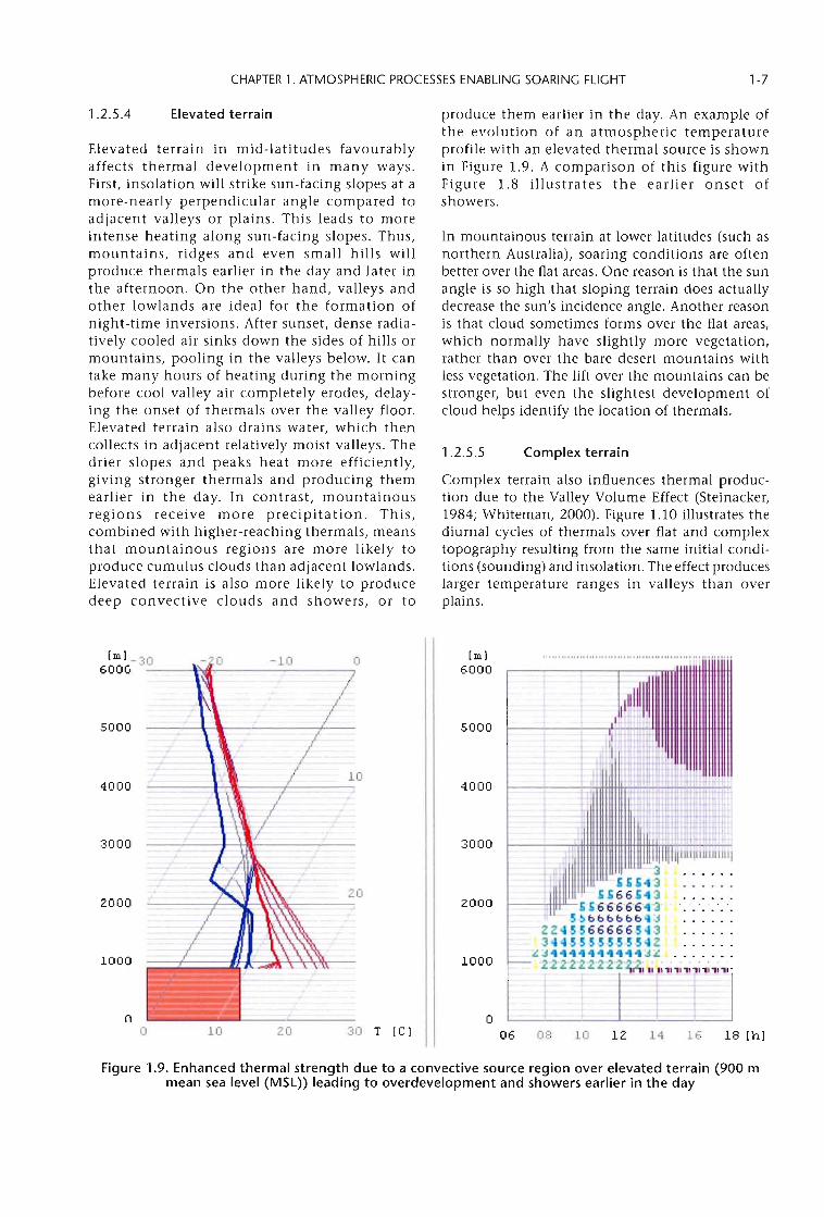
produce them earlier in the day. An example ofthe evolution of an atmospheric temperatureprofile with an elevated thermal source is shownin Figure 1.9. A comparison of this figure withFigure 1.8 illustrates the earlier onset ofshowers.
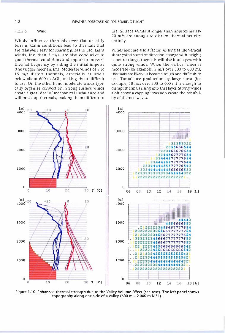
Complex terrain also influences thermal production due to the Valley Volume Effect (Steinacker,1984; Whiteman, 2000). Figure 1.10 illustrates thediurnal cycles of thermals over flat and complextopography resulting from the same initial conditions (sounding) and insolation. The effect produceslarger temperature ranges in valleys than overplains.
In mountainous terrain at lower latitudes (such asnorthern Australia), soaring conditions are oftenbetter over the flat areas. One reason is that the sunangle is so high that sloping terrain does actuallydecrease the sun's incidence angle. Another reasonis that cloud sometimes forms over the flat areas,which normally have slightly more vegetation,rather than over the bare desert mountains withless vegetation. The lift over the mountains can bestronger, but even the slightest development ofcloud helps identify the location of thermals.
Complex terrain1.2.5.5
Elevated terrain1.2.5.4
[Ill]
6000
4000
5000
10
3000 3000
3 ............UH3 .... - .....
20 U66H3 ................2000 2000 J; Ji 6"6"6'6'6'4'3' ..................
5~bbbbbb 'J ..................
ZZ45566666543 ..................
3H·55HH5HZ ...............
1000 1000 ~:J"""""""""".j~ ........................·.·2·;;.;~
n 00 10 20 30 T [Cl 06 08 10 12 14 16 18 [hI
[Ill)600G- 3_0__-P.fl..- -_1_O --,0
4000
5000
Figure 1.9. Enhanced thermal strength due to a convective source region over elevated terrain (900 mmean sea level (MSL)) leading to overdevelopment and showers earlier in the day
1-8 WEATHER FORECASTING FOR SOARING FLIGHT
1.2.5.6 Wind
Winds influence thermals over flat or hillyterrain. Calm conditions lead to thermals thatare relatively easy for soaring pilots to use. Lightwinds, less than 5 m/s, are also conducive togood thermal conditions and appear to increasethermal frequency by aiding the initial impulse(the trigger mechanism). Moderate winds of 5 toIS m/s distort thermals, especially at levelsbelow about 600 m AGL, making them difficultto use. On the other hand, moderate winds typically organize convection. Strong surface windscreate a great deal of mechanical turbulence andwill break up thermals, making them difficult to
use. Surface winds stronger than approximately20 m/s are enough to disrupt thermal activityentirely.
Winds aloft are also a factor. As long as the verticalshear (wind speed or direction change with height)is not too large, thermals will rise into layers withquite strong winds. When the vertical shear ismoderate (for example,S m/s over 300 to 600 m),thermals are likely to become rough and difficult touse. Turbulence production by large shear (forexample, 10 m/s over 300 to 600 m) is enough todisrupt thermals rising into that layer. Strong windsaloft above a capping inversion create the possibility of thermal waves.
[Ill]
400G-2_0_t=+===---tr--:=-~10[Ill]
4000
7t~_ ~235~~22T .Z3H666-5441---+--+--+Z'Z'3'4'6'6'6?6'6'-5'4
3ZU 5677776-54~~444577777654
~~4445U77777644
.Z3344444-5-5577776-543'3'33"4'4'4 'H'4"4'-5'6'6'6'6'6'-5'3'3
223~33333~333455554322
222222222222222222
3000
2000
1000
o06 08 10 12 14 16 18 [hI
20
30 T [Cl2010on
2000
1000
3000
[Ill]400G- 2_0--'''-=--.-__---,h- -,10
[Ill] ,.. , , , " .. ,.
4000
3000
2000
1000
J-f--
L
20
........ ~3000 '-5'-5'6'6'6'6'-5'-5'3
.Z ZZZZZ3 -566677776-542~2222233556677777775..2 232233 .. 566777777765 ..333Z3Z3 -566677777776-53
2000 . 'Z'3'Z'Z'Z'Z'3' '$'6'6'6?7'777'7'7'6'$'3.. ZZ ZZZ3 $-5666666666$4Z
22223455666666666542.. 22333455555555555.. 3.. Z ZZ334 $$-5-5-5$$$$$4Z
1000 ." 'Z'Z'3'3'3' '4' . . , '4' , '4' . '4'3'Z'.222~33333""""4"44"32
2222222222222222222
no 10 20 30 T [Cl
o06 08 10 12 14 16 18 [hI
Figure 1.10. Enhanced thermal strength due to the Valley Volume Effect (see text). The left panel showstopography along one side of a valley (500 m - 2 000 m MSL).
CHAPTER 1. ATMOSPHERIC PROCESSES ENABLING SOARING FLIGHT 1-9
Cool or stable low-level air can drift with the wind.Thus, some landforms can reduce or eliminate thermal activity, for example, downwind of large lakesor wet irrigated areas. These "dead air" regions arerevealed by cloudless areas in an otherwise cumulus-filled sky.
There is a significant difference between convective soaring conditions in Australia and Europe.In Europe the best conditions are often on theday after the cold front passage, while in Australia,the best day normally is the day just before thecold front passage, or even better, the day of thecold front passage (provided the passage happensin the evening or night). In simple terms, thisprobably means that in Europe, the change in thelapse rate (or stability) is the deciding factor,while in Australia the deciding factor is theextreme heating of the underlying surface (andthe consequently increasing temperatures in thesurface layer).
1.2.7 A pilot's view: a flight in thermallift
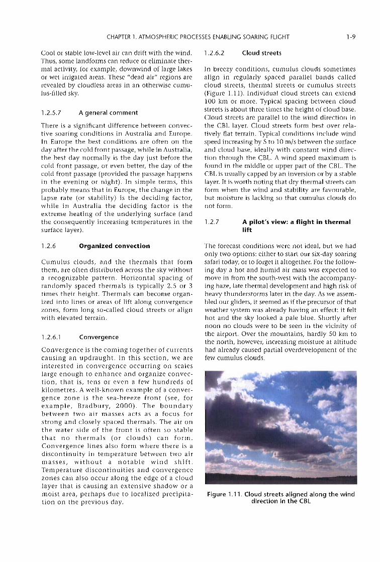
In breezy conditions, cumulus clouds sometimesalign in regularly spaced parallel bands calledcloud streets, thermal streets or cumulus streets(Figure 1.11). Individual cloud streets can extend100 km or more. Typical spacing between cloudstreets is about three times the height of cloud base.Cloud streets are parallel to the wind direction inthe CBL layer. Cloud streets form best over relatively flat terrain. Typical conditions include windspeed increasing by 5 to 10 m/s between the surfaceand cloud base, ideally with constant wind direction through the CBL. A wind speed maximum isfound in the middle or upper part of the CBL. TheCBL is usually capped by an inversion or by a stablelayer. It is worth noting that dry thermal streets canform when the wind and stability are favourable,but moisture is lacking so that cumulus clouds donot form.
Cloud streets1.2.6.2
A general comment1.2.5.7
1.2.6 Organized convection
Cumulus clouds, and the thermals that formthem, are often distributed across the sky withouta recognizable pattern. Horizontal spacing ofrandomly spaced thermals is typically 2.5 or 3times their height. Thermals can become organized into lines or areas of lift along convergencezones, form long so-called cloud streets or alignwith elevated terrain.
Convergence is the coming together of currentscausing an updraught. In this section, we areinterested in convergence occurring on scaleslarge enough to enhance and organize convection, that is, tens or even a few hundreds ofkilometres. A well-known example of a convergence zone is the sea-breeze front (see, forexample, Bradbury, 2000). The boundarybetween two air masses acts as a focus forstrong and closely spaced thermals. The air onthe water side of the front is often so stablethat no thermals (or clouds) can form.Convergence lines also form where there is adiscontinuity in temperature between two airmasses, without a notable wind shift.Temperature discontinuities and convergencezones can also occur along the edge of a cloudlayer that is causing an extensive shadow or amoist area, perhaps due to localized precipitation on the previous day.
Figure 1.11. Cloud streets aligned along the winddirection in the CBL
The forecast conditions were not ideal, but we hadonly two options: either to start our six-day soaringsafari today, or to forget it altogether. For the following day a hot and humid air mass was expected tomove in from the south-west with the accompanying haze, late thermal development and high risk ofheavy thunderstorms later in the day. As we assembled our gliders, it seemed as if the precursor of thatweather system was already haVing an effect: it felthot and the sky looked a pale blue. Shortly afternoon no clouds were to be seen in the vicinity ofthe airport. Over the mountains, hardly 50 km tothe north, however, increasing moisture at altitudehad already caused partial overdevelopment of thefew cumulus clouds.
Convergence1.2.6.1
1-10 WEATHER FORECASTING FOR SOARING FLIGHT
As soon as I stuffed my toothbrush and sleeping bagbehind the seat, I rolled the glider out to therunway. Nobody wanted to take off into cloudlessconditions around the airfield, so I got a tow rightaway. "Go north, and I'll release when I think I canmake it to the clouds", I told the tow pilot. As weheaded north and climbed through the haze layerat 1 000 m, I could see the first shower under one ofthe fat cumulus congestus over the highest point ofthe mountains. After release 1 glided cautiouslytowards the least-developed cumulus in the entirepack of dense clouds, hoping to get there before itdumped its load of water.
As 1 climbed slowly, I saw that the clouds to thewest appeared to be ones shooting up most rapidly.Farther east I was able to penetrate the shower line.After another 30 km the cloud base rose from1 700 m mean sea level (MSL) to nearly 2 000 m,visibility was better and none of the cumulusclouds showed exceeding vertical development. Ifollowed a line of clouds, which was the result of aconvergence: the early thermal development overthe high hills drew in air from the wide basin inthe east and the lower river valley to the west.Along the line of collision of those two currents,strong updraughts bubbled up and formed a highway in the sky, which made for fast cruising. As Iapproached the end of this run, still close to cloudbase, I swung around to the upWind side of the lastcumulus to avoid getting sucked into its whitebelly. And, 10 and behold, rather than hittingdescending air found so often next to a well-developed updraught, I continued to climb. Soon I foundmyself 200 m above cloud base, at some distancefrom the white stuff. What a rare view. It felt likesoaring the ridge lift on a snowy slope. Most likely,a wind shear in the upper part of the convectionlayer had triggered this flow pattern with itsincrease in wind speed with altitude.
Much too soon this exhilarating part of the flightcame to an end and I entered the typical setup of apromising thermal day. Good-looking clouds withdark, flat bottoms scattered almost evenly acrossthe sky in front of me. Climbs of 3-4 m/s alternatedwith fast cruise of 160 km/h and made for excellentprogress. Two hours later another range of hillscame into view, the highest ridge reaching justabout 1 000 m. The stronger thermal conditionstypical for hilly terrain manifested themselves in amarkedly higher cloud base and more verticaldevelopment of the cumulus clouds. 1 sped up toget as quickly as possible to the promising conditions ahead. The first climb confirmed myexpectations: the variometer needle swung aroundthe 5 m/s mark, and when I stopped climbing to
proceed north-east I was at almost 3 000 m. Twomore boomers like this one and I was at the end ofthe ridge. I turned toward a more easterly courseand headed out over the adjoining plain. As itselevation was only about 150 m MSL, I was atroughly 2 800 m AGL, a rare situation in this part ofthe world. The air mass ahead was different: achange in visibility and hardly any cloud were asign of drastically reduced humidity. As much as Ienjoyed the view, I missed the clouds as makers ofupdraughts. After a long glide I found the next thermal at an altitude of about 1 200 m MSL. I barelymanaged to extract a paltry 1.5 m/so The blue conditions lived up to their reputation: the updraughtswere weaker, reached to lower top altitudes and, ontop, were more difficult to find. This was going tobe the slow part of the flight.
It was a blue line on the map that appeared to makeyet another change in convective characteristics:shortly after I crossed a big river, the blue of the skydeepened, the visibility seemed to be unlimitedand in the distance I saw a small cumulus floatinghigh over a green forest. I made one more cautiousclimb in the blue before I dared to glide out to thelittle cloud. It didn't disappoint. A constant climbat almost 3 m/s brought me up to 2 500 m. Noproblem to get centred properly in this updraught,it was a wide and quietly rising column of air: asurprisingly strong evening thermal! It was almost6 p.m. and my goal was an easy final glide away.After landing I quickly checked my flight recorder:620 km distance, it displayed. What a wonderfulflight!
1 .3 RIDGE LIFT
Ridge soaring (also called slope soaring) was thefirst source of rising air used by glider pilots tomaintain or gain altitude, allOWing flight forextended periods. Today, ridge soaring still proVidesa consistent source of lift in hilly or mountainousterrain when winds are favourable. Ridge soaring isuseful over the full spectrum of soaring flight - frombasic training to contests and record flying.
1.3.1 Mechanism
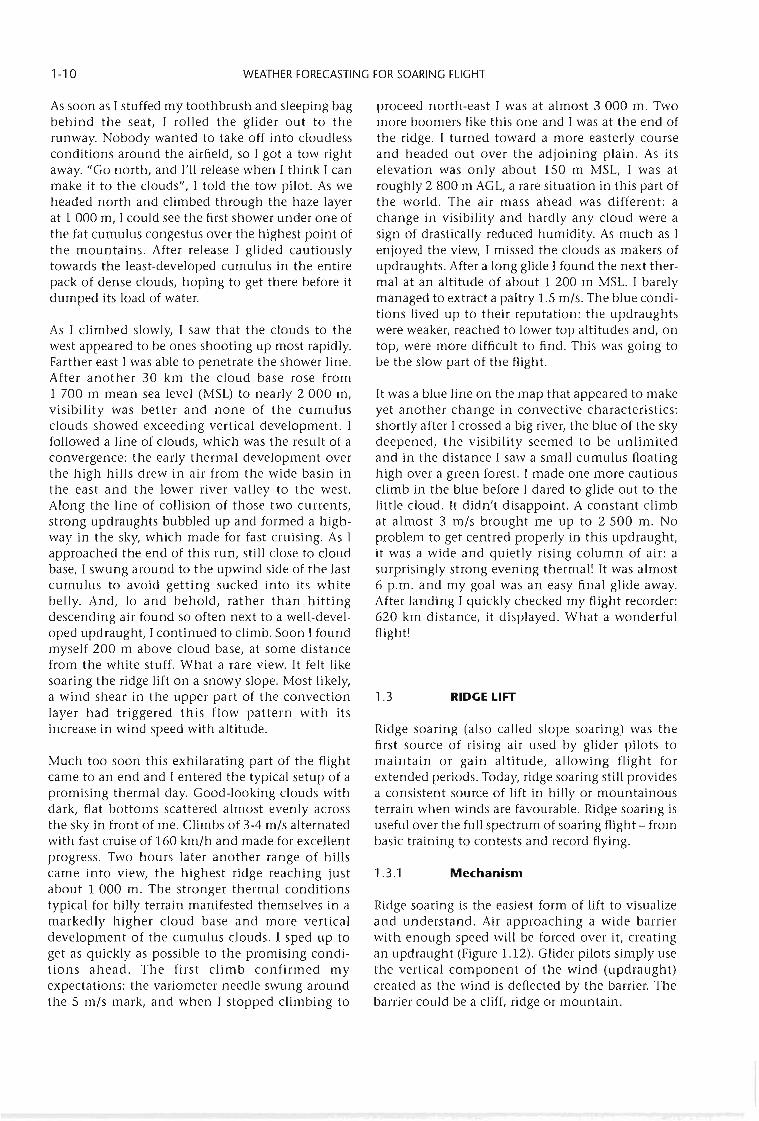
Ridge soaring is the easiest form of lift to visualizeand understand. Air approaching a wide barrierwith enough speed will be forced over it, creatingan updraught (Figure 1.12). Glider pilots simply usethe vertical component of the wind (updraught)created as the wind is deflected by the barrier. Thebarrier could be a cliff, ridge or mountain.
CHAPTER 1. ATMOSPHERIC PROCESSES ENABLING SOARING FLIGHT 1-11
The distribution of updraughts along the slopedepends on the wind speed and direction, stabilityof the air and nature of the slope itself (its shapeand texture). Unfortunately, these details are oftendifficult to quantify. Knowledge of local soaringexperts proVides valuable input to the weatherforecaster.
1.3.2 Meteorological factors
Wind is the critical meteorological ingredient forslope soaring. For moderate slopes (about 30°), aminimum wind speed of about 5 mjs blOWingtowards the ridge is needed. Stronger windsproduce stronger updraughts, but also createstronger turbulence, especially close to the slopeand on the lee side.
Ideally, the wind direction should be perpendicular to the ridge. Wind directions within 10° or20° of perpendicular also produce updraughts,but oblique wind angles are not useful. Eventhough a strong wind at an oblique angle shouldhave a sufficient component towards the ridge,updraughts are doubtful. The reason is that asthe wind angle deviates further from a directionperpendicular to the ridge line, there is anincreasing tendency for the flow to deflect andrun parallel to the ridge line. This process is morelikely if winds aloft, as well as at the surface, areoblique to the ridge.
Stability of the air mass plays a secondary role.Stable layers offer more resistance to verticaldisplacements. Thus, a neutral or only slightlystable layer will be lifted over a barrier more easily,proViding stronger and higher-reaching updraughtsfor ridge soaring.
Changes in wind direction with height force threedimensional thinking, especially in regions of highand complex terrain. For instance, the wind at lowlevels might be channelled along the valley, whileat mountaintop levels the wind is directed perpendicular to the mountains, producing updraughtsthere. Thus, in high, complex terrain it is importantto be aware of wind direction and speed at all levels.In addition, waves excited by upstream terrain cancause turbulence or sink where ridge lift wouldotherwise be expected.
Three factors are important in determining whetherflow will go over or around a barrier. First, thestronger the flow, the greater the tendency for airto go over, rather than around, the barrier. Second,air with neutral stability has a greater tendency toflow over a barrier; stable air tends to flow arounda barrier (see also the concept of the diVidingstreamline (Whiteman, 2000)). Third, the flowtends to go over wide barriers, while it flows aroundsmall or narrow barriers. These factors are combinedinto one parameter called the Froude number,which takes a variety of forms. The most useful
Figure 1.12. Wind blowing towards the rising terrain creates an updraught (arrows), called ridge or slopelift. Note: The grey line near the upwind ridge crest is the ground track of the glider.
1-12 WEATHER FORECASTING FOR SOARING FLIGHT
definition for our purposes is: speed of the flowdivided by the product of the flow stability andbarrier length. Readers seeking a more theoreticaltreatment of flows around barriers are directed tomany references on the Froude number in the literature (see, for example, Baines, 1995).
1.4 WAVE LIFT
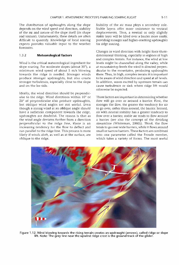
Mountain lee waves were first explored by soaringpilots in the Riesengebirge of Poland during the1930s (Dbrnbrack and others, 2006). The waveswere quickly recognized as a source for obtaininghigh altitudes, and by the early 1950s, glider pilotsusing mountain waves had reached the lower stratosphere. The world altitude record as of 2006 is15 460 m. Observations have shown evidence ofatmospheric waves extending to heights of 30 km.Mountain waves have also been used for manydistance and speed records. Notable among these isthe first soaring flight exceeding 3 000 kmachieved in 2003. Mountain waves occur worldwide in the lee of small and large topographicalbarriers (Figure 1.13).
1.4.1 Waves in the atmosphere: windand stability
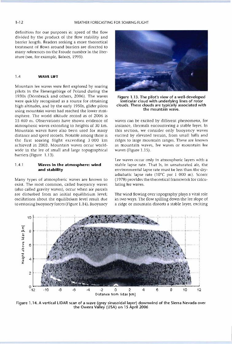
Many types of atmospheric waves are known toexist. The most common, called buoyancy waves(also called gravity waves), occur when air parcelsare disturbed from an initial equilibrium level;oscillations about the equilibrium level result dueto restoring buoyancy forces (Figure 1.14). Buoyancy
Figure 1.13. The pilot's view of a well-developedlenticular cloud with underlying lines of rotor
clouds. These clouds are typically associated withthe mountain wave.
waves can be excited by different phenomena, forinstance, thermals encountering a stable layer. Inthis section, we consider only buoyancy wavesexcited by elevated terrain, from small hills andridges to large mountain ranges. These are knownas mountain waves, lee waves or mountain leewaves (Figure 1.15).
Lee waves occur only in atmospheric layers with astable lapse rate. That is, in unsaturated air, theenvironmental lapse rate must be less than the dryadiabatic lapse rate (looe per 1 000 m). Scorer(1978) provides the theoretical framework for calculating lee waves.
The wind flowing over topography plays a vital rolein two ways. The flow spilling down the lee slope ofa ridge or mountain distorts a stable layer, exciting
121086·4 ·2 0 2 4Distance from lidar [km]
-6-8-10
.....................: ~:Ii
2
10
IQ
;gQ)
~ 6.£:lIQ....c.~ 4:c
Figure 1.14. A vertical L1DAR scan of a wave (grey sinusoidal layer) downwind of the Sierra Nevada overthe Dwens Valley (USA) on 15 April 2006
CHAPTER 1. ATMOSPHERIC PROCESSES ENABLING SOARING FLIGHT 1-13
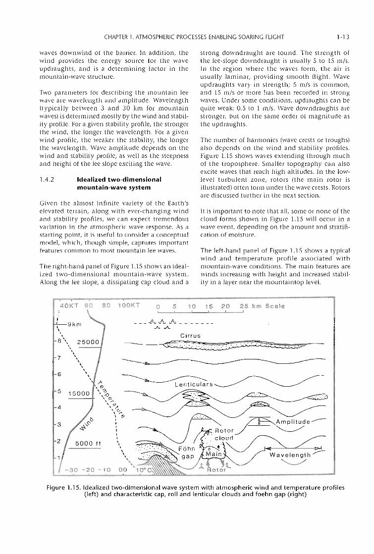
waves downwind of the barrier. In addition, thewind provides the energy source for the waveupdraughts, and is a determining factor in themountain-wave structure.
Two parameters for describing the mountain leewave are wavelength and amplitude. Wavelength(typically between 3 and 30 km for mountainwaves) is determined mostly by the wind and stability profile. For a given stability profile, the strongerthe wind, the longer the wavelength. For a givenwind profile, the weaker the stability, the longerthe wavelength. Wave amplitude depends on thewind and stability profile, as well as the steepnessand height of the lee slope exciting the wave.
1.4.2 Idealized two-dimensionalmountain-wave system
strong downdraught are found. The strength ofthe lee-slope downdraught is usually 5 to 15 m/soIn the region where the waves form, the air isusually laminar, providing smooth flight. Waveupdraughts vary in strength; 5 m/s is common,and 15 m/s or more has been recorded in strongwaves. Under some conditions, updraughts can bequite weak: 0.5 to 1 m/so Wave downdraughts arestronger, but on the same order of magnitude asthe updraughts.
The number of harmonics (wave crests or troughs)also depends on the wind and stability profiles.Figure 1.15 shows waves extending through muchof the troposphere. Smaller topography can alsoexcite waves that reach high altitudes. In the lowlevel turbulent zone, rotors (the main rotor isillustrated) often form under the wave crests. Rotorsare discussed further in the next section.
Given the almost infinite variety of the Earth'selevated terrain, along with ever-changing windand stability profiles, we can expect tremendousvariation in the atmospheric wave response. As astarting point, it is useful to consider a conceptualmodel, which, though simple, captures importantfeatures common to most mountain lee waves.
The right-hand panel of Figure 1.15 shows an idealized two-dimensional mountain-wave system.Along the lee slope, a dissipating cap cloud and a
It is important to note that all, some or none of thecloud forms shown in Figure 1.15 will occur in awave event, depending on the amount and stratification of moisture.
The left-hand panel of Figure 1.15 shows a typicalwind and temperature profile associated withmountain-wave conditions. The main features arewinds increasing with height and increased stability in a layer near the mountaintop level.
40KT 60 80 100KT 10 15 20 25 km Scale5
Lenticulars
Cirrus
-c:::z-::.....=::. -:.S5S-"..:.:t:=::s:: ! .. ?
o
___ AAA _..JI..A
5000 ft
.>-\ ~
\\~---+ \ ~, "..
" <:i>"
\ "'"..I ~I
•,,II,
\,\\
\
-30 -20 -10
4
5
7
6
3
, 9km\
\\
8 \\\
\\
\\ ,,,
\
",\
\
,,,
Figure 1.15. Idealized two-dimensional wave system with atmospheric wind and temperature profiles(left) and characteristic cap, roll and lenticular clouds and foehn gap (right)
1-14 WEATHER FORECASTING FOR SOARING FLIGHT
Turbulence below laminar flow is almost alwaysfound when mountain waves are strong enough tobe useful to soaring pilots. Soaring pilots use theterm rotor to refer to any turbulent air under thelaminar wave flow.
1.4.2.1 Turbulence associated with mountainwaves - Rotors and wave breaking
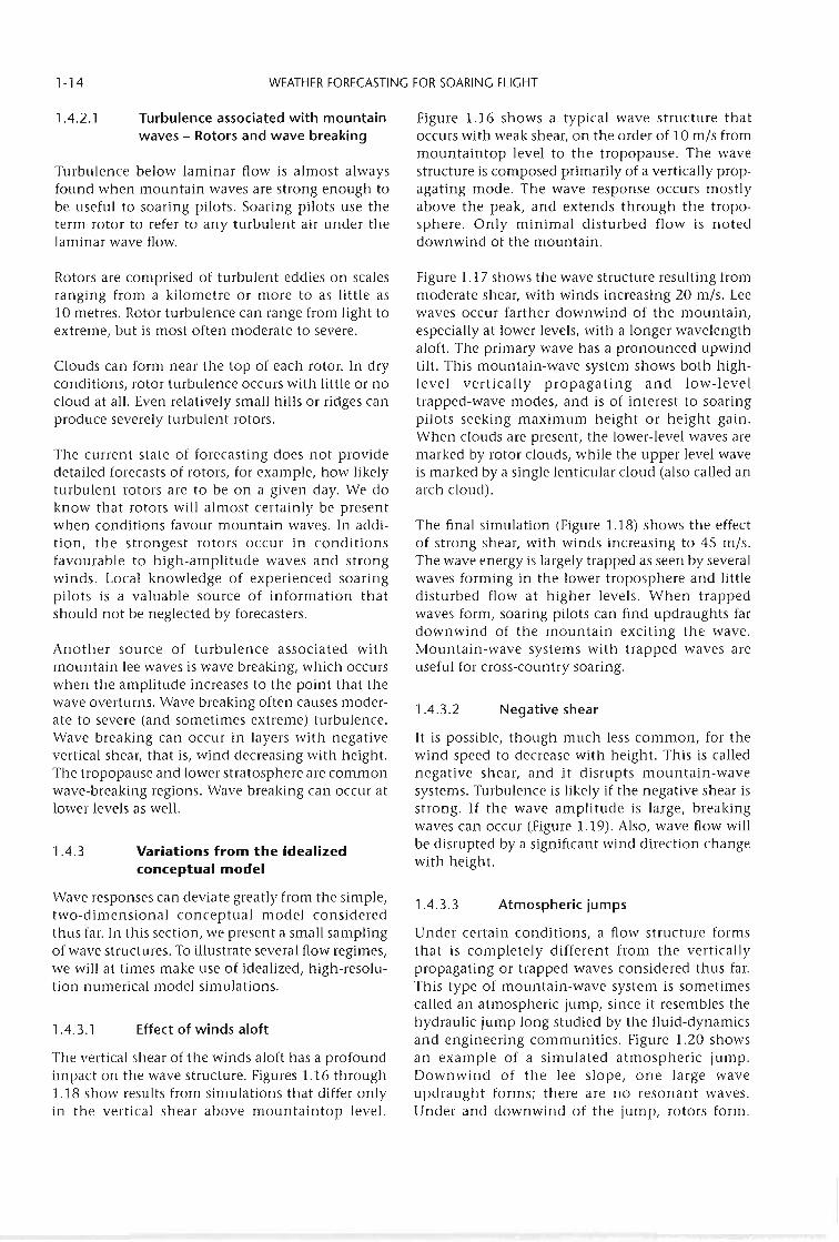
Figure 1.16 shows a typical wave structure thatoccurs with weak shear, on the order of 10 m/s frommountaintop level to the tropopause. The wavestructure is composed primarily of a vertically propagating mode. The wave response occurs mostlyabove the peak, and extends through the troposphere. Only minimal disturbed flow is noteddownwind of the mountain.
Rotors are comprised of turbulent eddies on scalesranging from a kilometre or more to as little as10 metres. Rotor turbulence can range from light toextreme, but is most often moderate to severe.
Clouds can form near the top of each rotor. In dryconditions, rotor turbulence occurs with little or nocloud at all. Even relatively small hills or ridges canproduce severely turbulent rotors.
The vertical shear of the winds aloft has a profoundimpact on the wave structure. Figures 1.16 through1.18 show results from simulations that differ onlyin the vertical shear above mountaintop level.
1.4.3 Variations from the idealizedconceptual model
Wave responses can deviate greatly from the simple,two-dimensional conceptual model consideredthus far. In this section, we present a small samplingof wave structures. To illustrate several flow regimes,we will at times make use of idealized, high-resolution numerical model simulations.
Negative shear
Atmospheric jumps
1.4.3.2
1.4.3.3
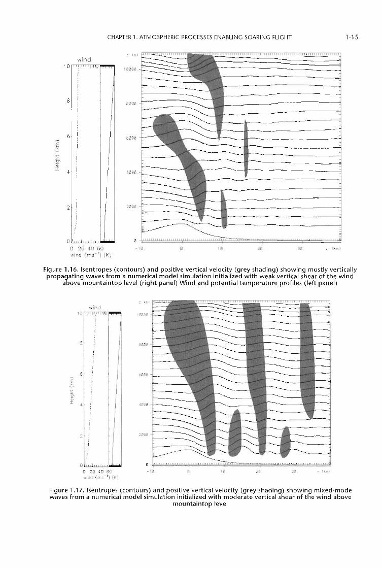
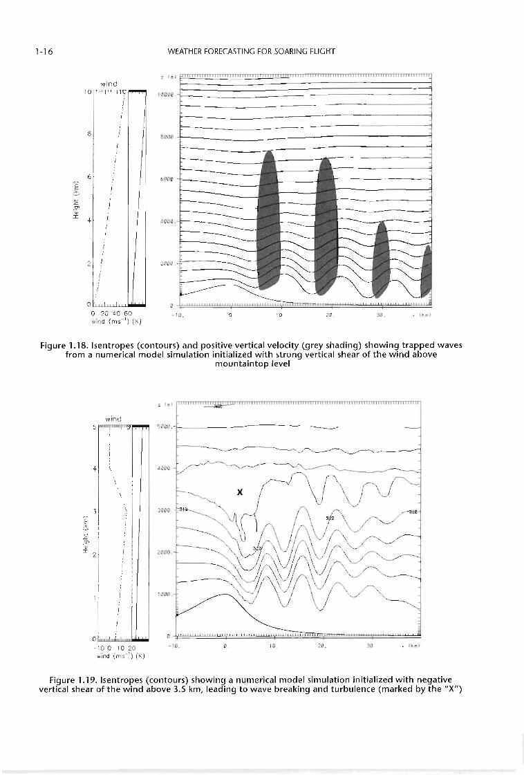
The final simulation (Figure 1.18) shows the effectof strong shear, with winds increasing to 45 m/soThe wave energy is largely trapped as seen by severalwaves forming in the lower troposphere and littledisturbed flow at higher levels. When trappedwaves form, soaring pilots can find updraughts fardownwind of the mountain exciting the wave.Mountain-wave systems with trapped waves areuseful for cross-country soaring.
Figure 1.17 shows the wave structure resulting frommoderate shear, with winds increasing 20 m/so Leewaves occur farther downwind of the mountain,especially at lower levels, with a longer wavelengthaloft. The primary wave has a pronounced upwindtilt. This mountain-wave system shows both highlevel vertically propagating and low-leveltrapped-wave modes, and is of interest to soaringpilots seeking maximum height or height gain.When clouds are present, the lower-level waves aremarked by rotor clouds, while the upper level waveis marked by a single lenticular cloud (also called anarch cloud).
It is possible, though much less common, for thewind speed to decrease with height. This is callednegative shear, and it disrupts mountain-wavesystems. Turbulence is likely if the negative shear isstrong. If the wave amplitude is large, breakingwaves can occur (Figure 1.19). Also, wave flow willbe disrupted by a significant wind direction changewith height.
Under certain conditions, a flow structure formsthat is completely different from the verticallypropagating or trapped waves considered thus far.This type of mountain-wave system is sometimescalled an atmospheric jump, since it resembles thehydraulic jump long studied by the fluid-dynamicsand engineering communities. Figure 1.20 showsan example of a simulated atmospheric jump.Downwind of the lee slope, one large waveupdraught forms; there are no resonant waves.Under and downwind of the jump, rotors form.
Effect of winds aloft
The current state of forecasting does not proVidedetailed forecasts of rotors, for example, how likelyturbulent rotors are to be on a given day. We doknow that rotors will almost certainly be presentwhen conditions favour mountain waves. In addition, the strongest rotors occur in conditionsfavourable to high-amplitude waves and strongwinds. Local knowledge of experienced soaringpilots is a valuable source of information thatshould not be neglected by forecasters.
Another source of turbulence associated withmountain lee waves is wave breaking, which occurswhen the amplitude increases to the point that thewave overturns. Wave breaking often causes moderate to severe (and sometimes extreme) turbulence.Wave breaking can occur in layers with negativevertical shear, that is, wind decreasing with height.The tropopause and lower stratosphere are commonwave-breaking regions. Wave breaking can occur atlower levels as well.
1.4.3.1
CHAPTER 1. ATMOSPHERIC PROCESSES ENABLING SOARING FLIGHT 1-15
wind10 rTTl:'IlTT"Inr'lTT"WU"T"-"-""-
i
8
6
?-""~
+-'-'=Q'
VI
4-
2
o 1 I ..l..I.
o 20 40 50wind (ms-') (I<)
Figure 1.16. Isentropes (contours) and positive vertical velocity (grey shading) showing mostly verticallypropagating waves from a numerical model simulation initialized with weak vertical shear of the wind
above mountaintop level (right panel) Wind and potential temperature profiles (left panel)
wind10 rTTTTTnI: rlfT'lvT"l"'T"-"'T"-"TT-
r
8
6
E.:":-::=0'vI
4
2 )
)
I
o ,I ,I ~
o 20 40 50, ind (rrs- I
) (K)
100[10.
8~00
400--.=-__
-10 10. 2e 3ll. .- Ib'll
Figure 1.17. Isentropes (contours) and positive vertical velocity (grey shading) showing mixed-modewaves from a numerical model simulation initialized with moderate vertical shear of the wind above
mountaintop level
1-16 WEATHER FORECASTING FOR SOARING FLIGHT
10 1 II\J"T"T"T"T" 100 B.-r---- -------------------j/
880 8.t---- ~---------------~
6 0000.~
.§
...-
..c:0'.;;;:r:
4- 40 O.
2 I 2088.
o ,I 1 u.l.
o 20 40 50wind (rns- I
) (K)-18. 0. 10. 28. 3Il.
Figure 1.18. Isentropes (contours) and positive vertical velocity (grey shading) showing trapped wavesfrom a numerical model simulation initialized with strong vertical shear of the wind above
mountaintop level
z r. 1 fTTTlmTmTrr:r:r:W:!llImTTTTTTTTTTTTTTTTTTTTTTTTTTTTTTTTTnTTTTTTTTTTTTTTTITITTTTTITITITITITITTTIl
wind5 5000.{-- ~~---~
4- 4000
3 3008
f~...,.c0''q;:r:
2 2000.
I 1000.
r
28.10.o.0~~~~~~~~~~~~~~~~~~-10.
olau.wlwlwl.w.w~.w
-100 10 20wind (rns- I
) (K)
Figure 1.19. Isentropes (contours) showing a numerical model simulation initialized with negativevertical shear of the wind above 3.5 km, leading to wave breaking and turbulence (marked by the "X")
CHAPTER 1. ATMOSPHERIC PROCESSES ENABLING SOARING FLIGHT 1-1 7
wind10 rTTTTTTlrr"lrTt'1U""
J
8
6
I:c'"'q;
I4
2
o .i. .J..L.
o 20 40 60wind (ms-I) (K)
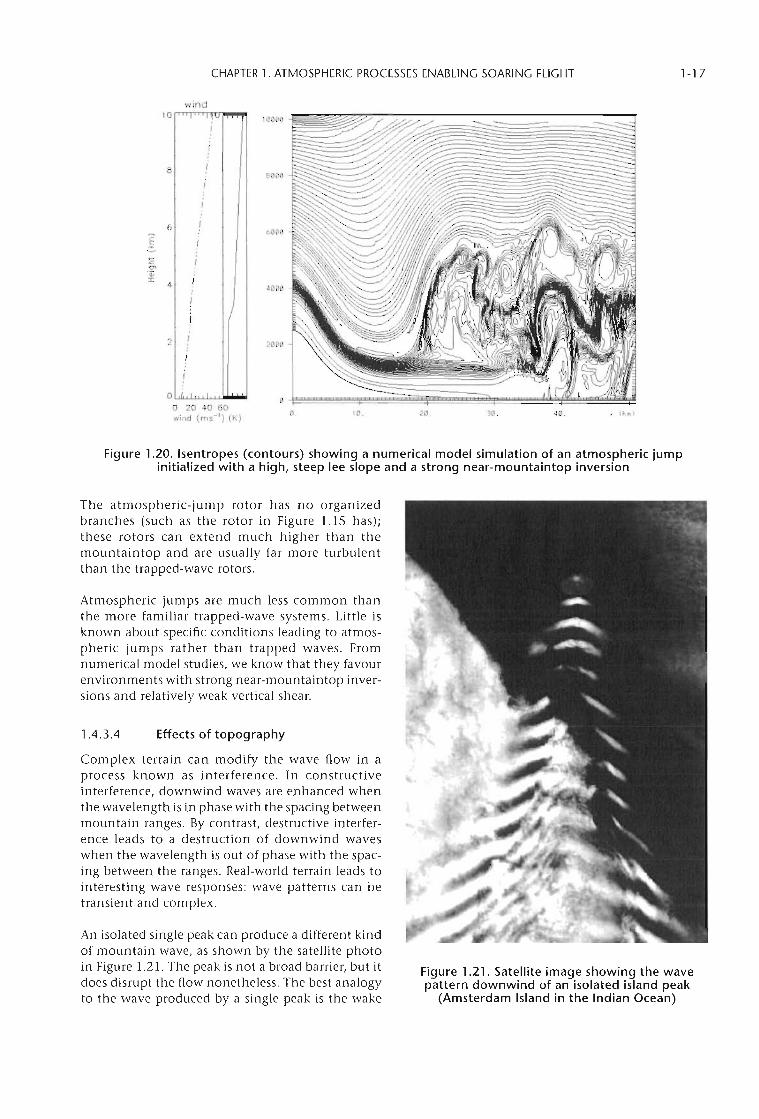
Figure 1.20. Isentropes (contours) showing a numerical model simulation of an atmospheric jumpinitialized with a high, steep lee slope and a strong near-mountaintop inversion
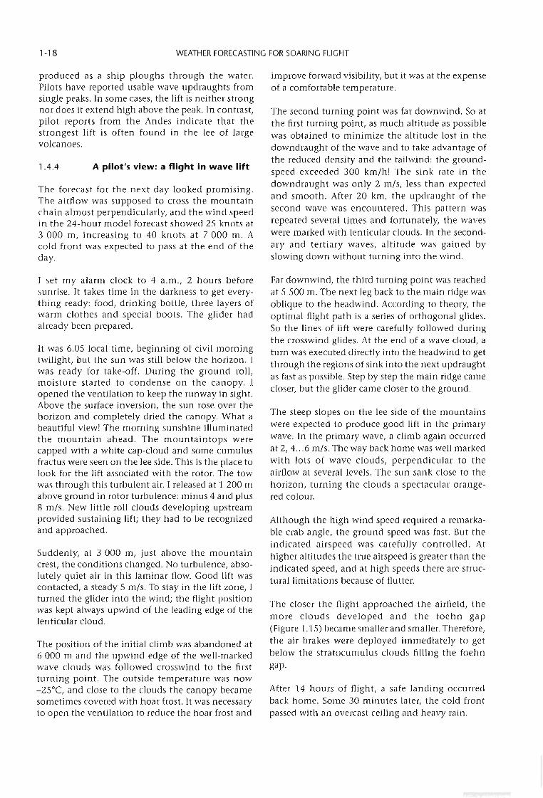
An isolated single peak can produce a different kindof mountain wave, as shown by the satellite photoin Figure 1.21. The peak is not a broad barrier, but itdoes disrupt the flow nonetheless. The best analogyto the wave produced by a single peak is the wake
The atmospheric-jump rotor has no organizedbranches (such as the rotor in Figure 1.15 has);these rotors can extend much higher than themountaintop and are usually far more turbulentthan the trapped-wave rotors.
Atmospheric jumps are much less common thanthe more familiar trapped-wave systems. Little isknown about specific conditions leading to atmospheric jumps rather than trapped waves. Fromnumerical model studies, we know that they favourenvironments with strong near-mountaintop inversions and relatively weak vertical shear.
Figure 1.21. Satellite image showing the wavepattern downwind of an isolated island peak
(Amsterdam Island in the Indian Ocean)
Effects of topography
Complex terrain can modify the wave flow in aprocess known as interference. In constructiveinterference, downwind waves are enhanced whenthe wavelength is in phase with the spacing betweenmountain ranges. By contrast, destructive interference leads to a destruction of downwind waveswhen the wavelength is out of phase with the spacing between the ranges. Real-world terrain leads tointeresting wave responses: wave patterns can betransient and complex.
1.4.3.4
1-18 WEATHER FORECASTING FOR SOARING FLIGHT
produced as a ship ploughs through the water.Pilots have reported usable wave updraughts fromsingle peaks. In some cases, the lift is neither strongnor does it extend high above the peak. In contrast,pilot reports from the Andes indicate that thestrongest lift is often found in the lee of largevolcanoes.
1.4.4 A pilot's view: a flight in wave lift
The forecast for the next day looked promising.The airflow was supposed to cross the mountainchain almost perpendicularly, and the wind speedin the 24-hour model forecast showed 25 knots at3 000 m, increasing to 40 knots at 7 000 m. Acold front was expected to pass at the end of theday.
I set my alarm clock to 4 a.m., 2 hours beforesunrise. It takes time in the darkness to get everything ready: food, drinking bottle, three layers ofwarm clothes and special boots. The glider hadalready been prepared.
It was 6.05 local time, beginning of civil morningtwilight, but the sun was still below the horizon. Iwas ready for take-off. During the ground roll,moisture started to condense on the canopy. Iopened the ventilation to keep the runway in sight.Above the surface inversion, the sun rose over thehorizon and completely dried the canopy. What abeautiful view! The morning sunshine illuminatedthe mountain ahead. The mountaintops werecapped with a white cap-cloud and some cumulusfractus were seen on the lee side. This is the place tolook for the lift associated with the rotor. The towwas through this turbulent air. I released at 1 200 mabove ground in rotor turbulence: minus 4 and plus8 m/so New little roll clouds developing upstreamprovided sustaining lift; they had to be recognizedand approached.
Suddenly, at 3 000 m, just above the mountaincrest, the conditions changed. No turbulence, absolutely quiet air in this laminar flow. Good lift wascontacted, a steady 5 m/so To stay in the lift zone, Iturned the glider into the wind; the flight positionwas kept always upwind of the leading edge of thelenticular cloud.
The position of the initial climb was abandoned at6 000 m and the upwind edge of the well-markedwave clouds was followed crosswind to the firstturning point. The outside temperature was now-25°C, and close to the clouds the canopy becamesometimes covered with hoar frost. It was necessaryto open the ventilation to reduce the hoar frost and
improve forward visibility, but it was at the expenseof a comfortable temperature.
The second turning point was far downwind. So atthe first turning point, as much altitude as possiblewas obtained to minimize the altitude lost in thedowndraught of the wave and to take advantage ofthe reduced density and the tailwind: the groundspeed exceeded 300 km/hi The sink rate in thedowndraught was only 2 m/s, less than expectedand smooth. After 20 km, the updraught of thesecond wave was encountered. This pattern wasrepeated several times and fortunately, the waveswere marked with lenticular clouds. In the secondary and tertiary waves, altitude was gained byslowing down Without turning into the wind.
Far downwind, the third turning point was reachedat 5 500 m. The next leg back to the main ridge wasoblique to the headwind. According to theory, theoptimal flight path is a series of orthogonal glides.So the lines of lift were carefully followed duringthe crosswind glides. At the end of a wave cloud, aturn was executed directly into the headwind to getthrough the regions of sink into the next updraughtas fast as possible. Step by step the main ridge camecloser, but the glider came closer to the ground.
The steep slopes on the lee side of the mountainswere expected to produce good lift in the primarywave. In the primary wave, a climb again occurredat 2,4".6 m/so The way back home was well markedwith lots of wave clouds, perpendicular to theairflow at several levels. The sun sank close to thehorizon, turning the clouds a spectacular orangered colour.
Although the high wind speed required a remarkable crab angle, the ground speed was fast. But theindicated airspeed was carefully controlled. Athigher altitudes the true airspeed is greater than theindicated speed, and at high speeds there are structurallimitations because of flutter.
The closer the flight approached the airfield, themore clouds developed and the foehn gap(Figure 1.15) became smaller and smaller. Therefore,the air brakes were deployed immediately to getbelow the stratocumulus clouds filling the foehngap.
After 14 hours of flight, a safe landing occurredback home. Some 30 minutes later, the cold frontpassed with an overcast ceiling and heavy rain.
CHAPTER 1. ATMOSPHERIC PROCESSES ENABLING SOARING FLIGHT 1-19
With the exception of convergence acting to organize convection, we have only discussed lift sourcesin isolation. In many cases, two or more lift sourcesexist at the same time, and processes even interactwith each other.
In addition to convergence, ridge and wave lift alsocan act as a thermal source region and organizer.Thermals will be best and more numerous wherethey coincide with the updraught regions of theseother lift sources, and they will be suppressed indowndraught regions.
An uncommon phenomenon sometimes occurs, inwhich convective cloud streets are aligned acrossone or more mountain ranges with mountain waveabove, marked by lenticular clouds aligned parallelto the terrain. Hindman and others (2004) presentan analysis of one such case.
Both ridge and wave lift require elevated terrainand wind. The combination of lift sources providessoaring pilots a potential path into the wave fromlower levels. In areas with complex terrain, an unfavourable phasing of waves excited by an upwindbarrier can cancel lift on an otherwise lift-producing ridge.
We close this chapter by noting that the currentstate of our knowledge is incomplete. Over the past80 or 90 years, soaring pilots have identified liftsources that can be categorized as convection,convergence, ridge, wave or some combination ofthese. It is not uncommon, however, for the soaring pilot to report lift with characteristics, or in abackground environment, that does not fit ourcurrent conceptual models. It is possible that in thefuture, reports from soaring flights, combined withatmospheric research, will identify other, yetunknown, lift sources.
As we drove out to the airport, the sky offered arange of possible scenarios for our afternoon flight.There were cumulus clouds above the mountains,indicating thermal activity. There was a blusterywind coming from the west and shaking the motorglider in her tiedowns, so with the mountainous
Glider flight by dynamic soaring in a wind-shearsituation is theoretically possible for gliders(Lissaman, 2007), but it is not practised.
1.5.3 A pilot's view: a flight incombined lift
1.5.2 Other possibilities
Another wave-like lift source is a travelling wavesuch as a bore. An example that has been used bysoaring pilots is the Morning Glory of Australia(Pretor-Phinney, 2006). Occasionally, other occurrences of apparent travelling waves have beenreported in the soaring literature.
1.5.1 Convective waves
In flat terrain, waves can be excited above a CBL bythermals disturbing the overlying stable air, aphenomenon called convective waves. These formin an environment with a CBL capped by a stronginversion, along with relatively strong wind andshear in the stable air above. Convective waves areneither as strong nor reach as high as mountainwaves, but they have been measured at heightsmany times the depth of the CBL (Kuettner andothers, 1987). Convective waves can be randomlyorganized. Under certain conditions, however, thewind profile through the CBL is conducive to cloudstreets. Long lines of convective waves can thenform if the wind direction in the overlying stableair is perpendicular to that in the CBL.
the middle of the day, followed by wave redeveloping as convection dies away towards the end of theday.
COMBINED LIFT AND OTHER LIFTSOURCES
In complex terrain, or in regions with elevatedterrain bordering plains, it is possible for thermals,convergence and ridge and wave lift to exist on thesame day. It is also possible for one lift source toexist during part of the day, while others are presentduring other times. An example (found during thefall and spring in areas with relatively low terrain) iswave during the morning hours and thermals in
In elevated terrain, in an environment with relatively strong winds aloft, along with weak stabilityand strong insolation in lower levels, waves canexist above an active CBL. Rough thermals typicallywill be found along the rising, upwind branches ofrotors, possibly triggered by low-level convergenceassociated with rotors. Thus, an active CBL canprovide a pathway for entry into the wave.
A combination of elevated terrain, an environmentwith moderate winds and weak stability, along withsufficient insolation, leads to the simultaneousoccurrence of ridge lift and thermals. This is usefulto the soaring pilot since thermals often 11 cycle",that is, they cease to form for a period. When thisoccurs, soaring pilots can stay aloft using the ridgelift until thermals once again form.
1.5
1-20 WEATHER FORECASTING FOR SOARING FLIGHT
terrain surrounding us, ridge lift was almost a given.And with wind and mountains, there's always achance for lee waves.
When my pilot lined up the motorglider fortake-off, the last wind check read 20 knots at270 degrees. 'Tll show you the Route of theSeven Lakes, from a ridge perspective", my pilotdecided. Sure, this was Argentina, the mountains were the Andes - no point in chasingcommon thermals, when something much moreindigenous to place and meteorological conditions was on the menu.
The popular sightseeing trip connects seven lakeswith a road winding its way through a 90-kmstretch of valleys and passes, some deep andnarrow, others wide and open. It runs more or lessnorth-south, so the adjoining ridges would bemostly perpendicular to the westerly winds, offering a good chance for decent ridge lift. To get tothe beginning of our scenic flight, however, was adifferent story. We had to follow a valley more orless parallel to the wind, with little promise ofencountering lift-producing slopes. After a climbto 2 000 m, which brought us 10 km closer to ourstarting point, we turned off the engine andpointed the nose into a sun-facing bowl with asmall outcropping to the north. Mild turbulenceindicated that the air was alive. A little searchingand we found the sweet spot, where the windhitting the small ridge and the thermal energycollected by the bowl collaborated to form anupdraught, which lifted us at 2 m/s to the crest ofChapelco Mountain at 2 200 m. At the windwardside of the plateau next to the summit, plumes ofdust were kicked up and driven across, providing afirst visible confirmation of the forecast wind.
We swung around to the steep west-facing slopeand immediately felt the upward push of the ridgelift. No need to fly back and forth along the ridge togain altitude - one slight pull up in the strongestpart of the updraught and we were well above ridgeline. In the steep valley below, the road meanderedin wide S-turns between isolated mountains, shortridges and small contributing valleys. Seen fromour vantage point more than 1 000 m above, thistopography was anything but ideal for extendedridge soaring, where one looks for a long, smoothridge running perpendicular to the prevailing winddirection, with essentially flat and unobstructingterrain upwind of its slopes.
Our ridge ended as valley and road headed in thefirst S-bend turning west. Rather than jumping tothe next north-south slopes about 5 km ahead,
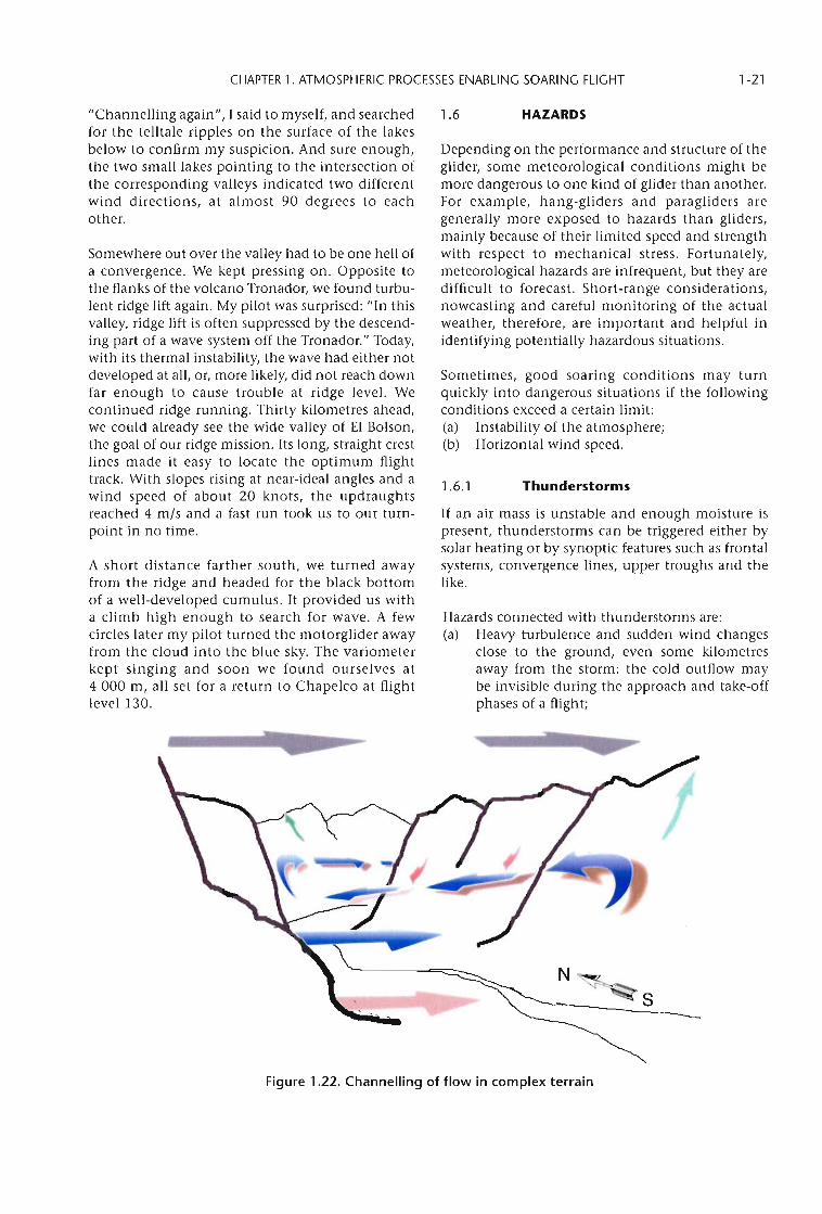
and accepting the probable altitude loss due tolee effects of the mountains across the valley, weturned west, too, crossing road and valley whileheading for a short, steep cliff pretty much parallel to the forecast wind direction. Amazinglyenough, we found lift there. Not the powerfulpush we felt before, but enough to keep us atconstant altitude, while cruising along at150 km/h. What was going on? "Always fly theouter perimeter of a turn in the valley!" my pilotcommented, as if talking to himself. Apparently,the complex, convoluted topography deflects thelocal flow so as to channel it into the direction ofappropriately aligned parts of valleys, even ifthey run at 90 degrees to the main wind direction. And this was the perfect demonstration:coming from the north, the valley curved westbefore completing its S-turn and opening into astraight section heading south again. The ridgeon its eastern flank rose to an almost constantaltitude of about 2 000 m and obviously proVidedthe deflecting barrier. If our channelling hypothesis was correct, then there wasn't muchdynamic lift to be expected from its slopes, asmost of the flow was not going to head uphill butrather "sideways", parallel to the valley floor(Figure 1.22).
And that was exactly what we found: no lift, justmild turbulence. We fell farther and farther belowthe ridge line. The valley widened and the middlepart of the slopes was covered with dense forest.After an agonizingly long descent we suddenly felta jolt. My pilot put the motorglider on its wingtipand muscled her into the tight core of a turbulentupdraught. This was not the typical mountainthermal. "Probably a mix of thermal, ridge lift androtor", he remarked, while trying to keep theairspeed between 130 and 150 km/h and maintaining a rather large distance to the slope. "This isa pretty dangerous combination if you're too closeto the ridge", he continued. "If the rotor pushesthe thermal just a little bit uphill, its downflowpart sits right where one would expect ridge lift.Fly there and you're doomed!" We took the roughupdraught just high enough to reach the nextridge farther south. On its smooth flank weencountered pure and strong uphill flow. Within acouple of kilometres we were well above crest line.Which is exactly what we needed: enough altitudeto safely cross Lago Nahuel Huapi and reach themountains on its south-western shore, about15 km away.
The first ridge on the other side we hit, althoughperfectly perpendicular to a westerly flow,produced nothing but strong downwash.
CHAPTER 1. ATMOSPHERIC PROCESSES ENABLING SOARING FLIGHT 1-21
"Channelling again", I said to myself, and searchedfor the telltale ripples on the surface of the lakesbelow to confirm my suspicion. And sure enough,the two small lakes pointing to the intersection ofthe corresponding valleys indicated two differentwind directions, at almost 90 degrees to eachother.
Somewhere out over the valley had to be one hell ofa convergence. We kept pressing on. Opposite tothe flanks of the volcano Tronador, we found turbulent ridge lift again. My pilot was surprised: "In thisvalley, ridge lift is often suppressed by the descending part of a wave system off the Tronador." Today,with its thermal instability, the wave had either notdeveloped at all, or, more likely, did not reach downfar enough to cause trouble at ridge level. Wecontinued ridge running. Thirty kilometres ahead,we could already see the wide valley of El Bolson,the goal of our ridge mission. Its long, straight crestlines made it easy to locate the optimum flighttrack. With slopes rising at near-ideal angles and awind speed of about 20 knots, the updraughtsreached 4 m/s and a fast run took us to our turnpoint in no time.
A short distance farther south, we turned awayfrom the ridge and headed for the black bottomof a well-developed cumulus. It provided us witha climb high enough to search for wave. A fewcircles later my pilot turned the motorglider awayfrom the cloud into the blue sky. The variometerkept singing and soon we found ourselves at4 000 m, all set for a return to Chapelco at flightlevel 130.
1.6 HAZARDS
Depending on the performance and structure of theglider, some meteorological conditions might bemore dangerous to one kind of glider than another.For example, hang-gliders and paragliders aregenerally more exposed to hazards than gliders,mainly because of their limited speed and strengthwith respect to mechanical stress. Fortunately,meteorological hazards are infrequent, but they aredifficult to forecast. Short-range considerations,nowcasting and careful monitoring of the actualweather, therefore, are important and helpful inidentifying potentially hazardous situations.
Sometimes, good soaring conditions may turnquickly into dangerous situations if the follOWingconditions exceed a certain limit:(a) Instability of the atmosphere;(b) Horizontal wind speed.
1.6.1 Thunderstorms
If an air mass is unstable and enough moisture ispresent, thunderstorms can be triggered either bysolar heating or by synoptic features such as frontalsystems, convergence lines, upper troughs and thelike.
Hazards connected with thunderstorms are:(a) Heavy turbulence and sudden wind changes
close to the ground, even some kilometresaway from the storm: the cold outflow maybe invisible during the approach and take-offphases of a flight;
Figure 1.22. Channelling of flow in complex terrain
1-22 WEATHER FORECASTING FOR SOARING FLIGHT
(b) Strong updraughts, whose climb rates can beso strong that the glider is sucked into thecloud. Paragliders and hang-gliders are especially susceptible;
(c) Strong downdraughts or downbursts: the sinkrate can cause an unexpected outlanding inunsuitable terrain associated with dangeroussurface wind conditions;
(d) Heavy precipitation, which can reduce thevisibility rapidly;
(e) Hail, which can cause serious damage to theglider in the air as well as on the ground;
(t) Lightning, which may also strike at somedistance from a storm. It is dangerous eitherto fly near or launch a glider in the vicinity ofa thunderstorm;
(g) Tornadoes, which are often associated withextreme thunderstorms and can damage tieddown gliders, trailers and even hangars;
(h) Icing in a thunderstorm, which can be sostrong that it becomes impossible to controlthe glider (in countries where cloud flying ispermitted).
1.6.2 Strong winds and wind shear
Whenever there is a wind blowing, there are likelyto be waves or slope conditions that glider pilotscan enjoy. But if the surface wind or the winds aloftexceed certain limits, soaring flight becomesincreasingly risky, depending on the type of glider.In addition, zones of significant wind shear or evena reversal in flow aloft can produce dangerousturbulence.
Hazards connected with strong winds are:(a) Strong drift: in connection with lee-wave
flow, little downwind drift may be noticedduring the climb. But at the wave crest, the
horizontal wind is strong and the sink rateincreases downwind of the crest. This causesa strong unexpected drift downwind, especially for less-experienced pilots. The resulting rapid loss of height can be dangerous,depending on the terrain and the cloudsbelow;
(b) Closing foehn gap (Figure 1.15): increasingmoisture, especially if there is a frontal systemapproaching, can close the foehn gap rapidly.If the pilot is not aware of the changing cloudcover below, the pilot could be in a criticalcondition;
(c) Severe downslope winds: the flow down thelee slope may be much stronger than upstreamof the ridge. Thus, flight in the lee of a ridgecan cause rapid loss of altitude and terrainclearance;
(d) Rotors (Figure 1.15) with heavy turbulencemake it sometimes impossible to control theglider;
(e) Wind shear on or near the ground below arotor: sometimes moving eddies alter thelow-level airflow. In foehn conditions, a coldpool of air near the ground and a strong windabove can produce a transition zone with astrong wind shear. In those conditions takeoff or landing can become unsafe;
(f) Wave breaking: regions of wind shear, especially a reversed flow, may destroy the wavesand produce heavy turbulence. (If not markedby clouds, this is called "clear air turbulence".)In these conditions, it can be difficult to keepthe glider within design speed limits;
(g) Orographic effects: flows through gaps ofmountains can accelerate the wind speedsignificantly (2-3 times more than the generalflow). The resulting downdraughts, windshear and turbulence can be serious.
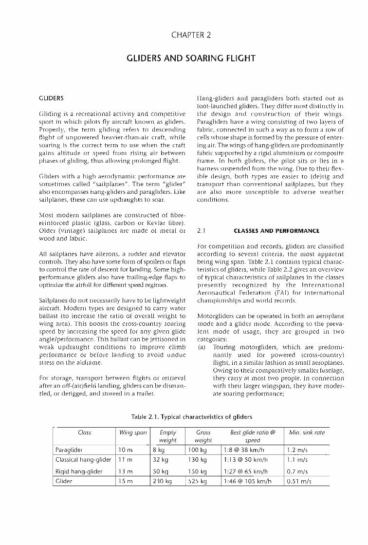
CHAPTER 2
GLIDERS AND SOARING FLIGHT
GLIDERS
Gliding is a recreational activity and competitivesport in which pilots fly aircraft known as gliders.Properly, the term gliding refers to descendingflight of unpowered heavier-than-air craft, whilesoaring is the correct term to use when the craftgains altitude or speed from rising air betweenphases of gliding, thus allOWing prolonged flight.
Gliders with a high aerodynamic performance aresometimes called "sailplanes". The term "glider"also encompasses hang-gliders and paragliders. Likesailplanes, these can use updraughts to soar.
Hang-gliders and paragliders both started out asfoot-launched gliders. They differ most distinctly inthe design and construction of their Wings.Paragliders have a wing consisting of two layers offabric, connected in such a way as to form a row ofcells whose shape is formed by the pressure of entering air. The wings of hang-gliders are predominantlyfabric supported by a rigid aluminium or compositeframe. In both gliders, the pilot sits or lies in aharness suspended from the wing. Due to their flexible design, both types are easier to (de)rig andtransport than conventional sailplanes, but theyare also more susceptible to adverse weatherconditions.
Most modern sailplanes are constructed of fibrereinforced plastic (glass, carbon or Kevlar fibre).Older (Vintage) sailplanes are made of metal orwood and fabric.
2.1 CLASSES AND PERFORMANCE
All sailplanes have ailerons, a rudder and elevatorcontrols. They also have some form of spoilers or flapsto control the rate of descent for landing. Some highperformance gliders also have trailing-edge flaps tooptimize the airfoil for different speed regimes.
Sailplanes do not necessarily have to be lightweightaircraft. Modern types are designed to carry waterballast (to increase the ratio of overall weight towing area). This boosts the cross-country soaringspeed by increasing the speed for any given glideangle/performance. This ballast can be jettisoned inweak updraught conditions to improve climbperformance or before landing to avoid unduestress on the airframe.
For storage, transport between flights or retrievalafter an off-(air)field landing, gliders can be dismantled, or derigged, and stowed in a trailer.
For competition and records, gliders are classifiedaccording to several criteria, the most apparentbeing wing span. Table 2.1 contains typical characteristics of gliders, while Table 2.2 gives an overviewof typical characteristics of sailplanes in the classespresently recognized by the InternationalAeronautical Federation (FA!) for internationalchampionships and world records.
Motorgliders can be operated in both an aeroplanemode and a glider mode. According to the prevalent mode of usage, they are grouped in twocategories:(a) Touring motorgliders, which are predomi
nantly used for powered (cross-country)flight, in a similar fashion as small aeroplanes.OWing to their comparatively smaller fuselage,they carry at most two people. In connectionwith their larger wingspan, they have moderate soaring performance;
Table 2.1. Typical characteristics of gliders
Class Wing span Empty Gross Best glide ratio @ Min. sink rateweight weight speed
Paraglider 10 m 8 kg 100 kg 1:8 @ 38 km/h 1.2 m/s
Classical hang-glider llm 32 kg 130 kg 1:13@50km/h 1.1 m/s
Rigid hang-glider Bm 50 kg 150 kg 1:27 @ 65 km/h 0.7 m/s
Glider 15 m 230 kg 525 kg 1:46 @ 105 km/h 0.51 m/s
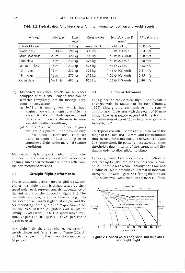
2-2 WEATHER FORECASTING FOR SOARING FLIGHT
Table 2.2. Typical values for glider classes for international competition and world records
FAI class Wing span Empty Gross weight Best glide ratio @ Min. sink rate
weight speed
Ultralight class Bm 110 kg max. 220 kg 1:37 @ 85 km/h 0.60 m/s
World class 13.44 m 190 kg 300 kg 1:33 @ 80 km/h 0.64 m/s
Multi-seat class 20 m 420 kg 700 kg 1:45 @ 103 km/h 0.58 m/s
Club class 15 m 230 kg 525 kg 1:40 @ 90 km/h 0.58 m/s
Standard class 15 m 230 kg 525 kg 1:44 @ 95 km/h 0.55 m/s
15 m class 15 m 230 kg 525 kg 1:46 @ 105 km/h 0.51 m/s
18 m class 18 m 270 kg 575 kg 1:50 @ 105 km/h 0.45 m/s
Open class No limit 480 kg 850 kg 1:65 @ 110 km/h 0.40 m/s
(b) Motorized sailplanes, which are sailplanesequipped with a small engine that can beretracted completely into the fuselage. Theycome in two variants:(i) Self-launch motorgliders, which have
engines powerful enough to enable theaircraft to take off, climb repeatedly andthus cover moderate distances in nonsoarable weather conditions;
(ii) Motorgliders with sustainer enginesthat are less powerful and provide onlylimited climb performance. They areuseful to avoid off-field landings or tocontinue a flight under marginal soaringconditions.
Many newer sailplanes, particularly in the 18-metreand open classes, are equipped with retractableengines, since their performance differs little fromthe non-motorized versions.
2.1.1 Straight-flight performance
2.1.2 Climb performance
For a glider in steady circular flight, the sink rate wchanges with the radius r of the turn (Thomas,1999). Slow gliders can climb in quite narrowatmospheric lift patterns with diameters of 30 m toSO m, while faster sailplanes need wider updraughtswith diameters of about 150 m in order to gain altitude (Figure 2.3).
The typical sink rate in circular flight is between therange of 0.8 m/s and 1.2 m/s, and the minimumtime needed for a full circle is between 10 sand20 s. Atmospheric lift patterns must exceed all thesethreshold values in terms of size, strength and lifetime in order to allow gliders to climb.
Typically, convection generates a lift pattern oflocalized updraughts centred around a core. A parabolic lift profile with a core updraught of 3 m/s anda radius of 150 m describes a thermal of moderatestrength quite well (Figure 2.4). Strong thermals areoften wider, while weak thermals are more confined.
Figure 2.1. Speed polars of gliders and sailplanesin straight flight
sink rate('pm]
·400
·200
6050
airspeed (mls)
30 402010oo""""':r--__.__-,----.-~--r~-,__~__.__-,----.-~__,
":......~------'.:.. ' ..::...........~~ open dass 1:65@ 110 km/h
" .......' '', ,..... standard ~Iass 1 44 @ 9S km/h
" ~ ,'" kr. tl \ ~
" " \ rigid hangglider 1:27@65km/h~, ,. .,dassical hangglider 1:13 50 km/h
\' 1).11 11de 8'gr ;\ \ \\ \ \\ \ \\ \ \
\ \ \\ \ \
-1
-2
.3 l.L.u...L.l..i-"-"-'-.LL.l.L.L.LL.1.J....o..L..J...LL.l.d.w..'-'-'-"'--'..J~..L.l..o.~.w.......~
o 25 50 75 100 125
airspeed (km/h]
sink rateImfs]
The aerodynamic performance of gliders and sailplanes in straight flight is characterized by theirspeed polar w(v), representing the dependence ofthe sink rate w on the airspeed v (Figure 2.1). Thebest glide ratio voJwo is obtained from a tangent tothe speed polar. This best glide ratio voh'vo and thecorresponding speed Vo are the major parametersfor the classification of gliders and sailplanes(Irving, 1998; Liechti, 2001). A speed range fromabout 75 per cent (stall speed) up to 250 per cent ofVo can be used.
In straight flight the glide ratio v/w decreases forspeeds slower and faster than Vo (Figure 2.2). Atdouble the speed of Vo the glide ratio is reduced toSO per cent.
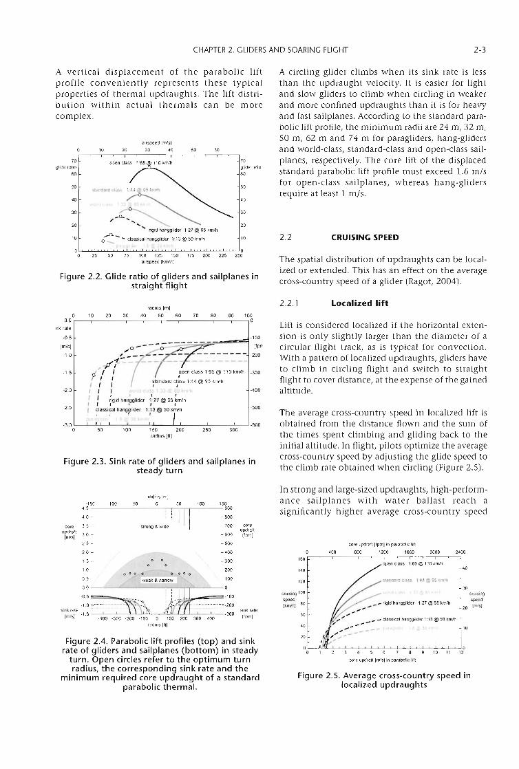
CHAPTER 2. GLIDERS AND SOARING FLIGHT 2-3
The spatial distribution of updraughts can be localized or extended. This has an effect on the averagecross-country speed of a glider (Ragot, 2004).
A circling glider climbs when its sink rate is lessthan the updraught velocity. It is easier for lightand slow gliders to climb when circling in weakerand more confined updraughts than it is for heavyand fast sailplanes. According to the standard parabolic lift profile, the minimum radii are 24 m, 32 m,50 m, 62 m and 74 m for paragliders, hang-glidersand world-class, standard-class and open-class sailplanes/ respectively. The core lift of the displacedstandard parabolic lift profile must exceed 1.6 m/sfor open-class sailplanes, whereas hang-glidersrequire at least 1 m/so
A vertical displacement of the parabolic liftprofile conveniently represents these typicalproperties of thermal updraughts. The lift distribution within actual thermals can be morecomplex.
airspeed [m/sI
10 20 30 40 50 60
70 open class 1:65@ 110 kmlh 70glide ratio glide ratio
60 60
50 50
40 40
30 30
20 20
10 10
0 00 25 50 75 100 125 150 175 200 225 250
airspeed {km/hi
Figure 2.2. Glide ratio of gliders and sailplanes instraight flight
2.2 CRUISING SPEED
2.2.1 Localized lift
Lift is considered localized if the horizontal extension is only slightly larger than the diameter of acircular flight track, as is typical for convection.With a pattern of localized updraughts, gliders haveto climb in circling flight and switch to straightflight to cover distance, at the expense of the gainedaltitude.
The average cross-country speed in localized lift isobtained from the distance flown and the sum ofthe times spent climbing and gliding back to theinitial altitude. In flight, pilots optimize the averagecross-country speed by adjusting the glide speed tothe climb rate obtained when circling (Figure 2.5).
-400
-500
300250150 200radius [ft]
10050
-100
,. 0 - - - ;:;:;.::.:::z::=::::=~~~"""'~, Irpn
, - - - - - - - - - - -200rll:"I'-:':'-:'_-=-- -------------
~;'~p'l I ~pen class 1:65 @ 110 kmlh -300
I : : itandard c~ass 1:44 @ 95 kmlh
, " i< ;,~ 1 2.:> IT 80 ~:l' I
I , ;i9id han~9lider 1':27 @ ;5 ~m/h, I I I J I
I classical hangplider \13 @ 50 km/h
-2.0
-1.5
-3.0 L----'----'-L....l'-----''----_-'--L_---'C-L__---'-__---L-------' -600o
-2.5
Figure 2.3. Sink rate of gliders and sailplanes insteady turn
radius (ml
o 10 20 30 40 50 60 70 80 90 100~O 0
·0.5
Imls]
-1.0
nk rale
Figure 2.4. Parabolic lift profiles (top) and sinkrate of gliders and sailplanes (bottom) in steady
turn. Open circles refer to the optimum turnradius, the corresponding sink rate and the
minimum required core updraught of a standardparabolic thermal.
0.0 -·-~------,.--___n~--O
-0.5 , d.;;j"..o-==_-100
-1.0 :.----------- - - ~11"'-- i- ----------: -200
sink rate 10 __lr'Imlsl -1.5 ~300 -200 -100 0 -'.J,0"'--OJ-2:-'-00c-'---:-3.L00~-300
radius 1ft]
40
30cruisingspeed
20 tm/s)
10
2400
standard c-ass 1 44 @ 95 km/h
open crass 1 65@ 110 kmlh
core updrafl (m/si in parabolic lift
core updrafllfpml in parabolic lilt
800 1200 1600 2000400
20
40
140
120
cruising 100
speed[km/hi 80
60
Figure 2.5. Average cross-country speed inlocalized updraughts
In strong and large-sized updraughts, high-performance sailplanes with water ballast reach asignificantly higher average cross-country speed
sink rale(rpml
150900
- 800
- 700 coreupdrafl
-600 (rpml
- 500
- 400
- 300
200
100
100
o 0 0 0
o 0
o
weak & narrow
o 0 0 0
radius [m)
·150 -100 -50 0 50
4.5---~,~4.0 - :
3.5 - slrong & wide
3.0 -
2.5 -
2.0 -
1.5 -
1.0
0.5
coreuJXlrarlIrn's)
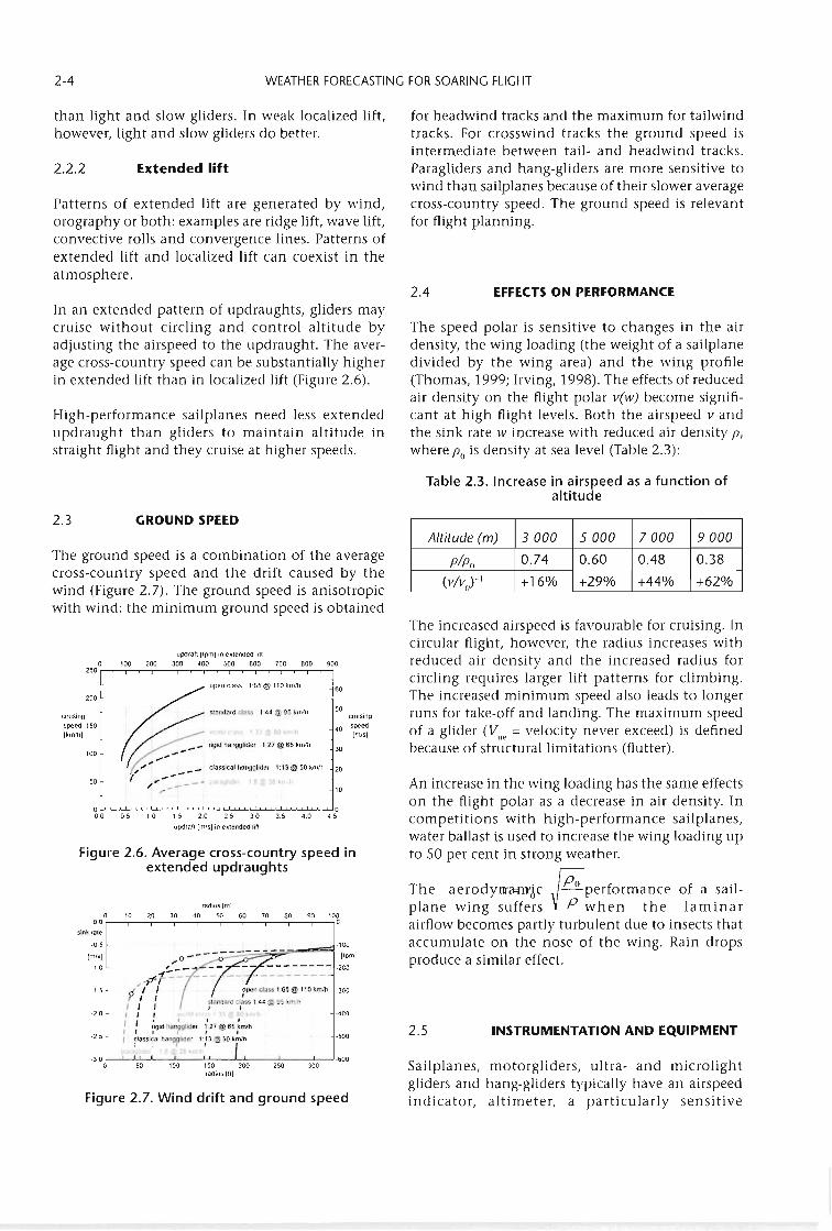
2-4 WEATHER FORECASTING FOR SOARING FLIGHT
for headwind tracks and the maximum for tailwindtracks. For crosswind tracks the ground speed isintermediate between tail- and headwind tracks.Paragliders and hang-gliders are more sensitive towind than sailplanes because of their slower averagecross-country speed. The ground speed is relevantfor flight planning.
than light and slow gliders. In weak localized lift,however, light and slow gliders do better.
2.2.2 Extended lift
Patterns of extended lift are generated by wind,orography or both: examples are ridge lift, wave lift,convective rolls and convergence lines. Patterns ofextended lift and localized lift can coexist in theatmosphere.
2.4 EFFECTS ON PERFORMANCEIn an extended pattern of updraughts, gliders maycruise without circling and control altitude byadjusting the airspeed to the updraught. The average cross-country speed can be substantially higherin extended lift than in localized lift (Figure 2.6).
High-performance sailplanes need less extendedupdraught than gliders to maintain altitude instraight flight and they cruise at higher speeds.
The speed polar is sensitive to changes in the airdensity, the wing loading (the weight of a sailplanedivided by the wing area) and the wing profile(Thomas, 1999; Irving, 1998). The effects of reducedair density on the flight polar v(w) become significant at high flight levels. Both the airspeed v andthe sink rate w increase with reduced air density P,where Po is density at sea level (Table 2.3):
Table 2.3. Increase in airspeed as a function ofaltitude
o 000 0.5 1 0 1.5 2.0 2.5 3.0 3.5 4.0 4.5
upjralt (m/s) in ex1ended lift
radiuslm!o 10 20 30 40 50 60 70 80 90 100
QO 0
updraft ('pm) In eKlended fill
o 100 200 300 400 500 600 700 800 900250 r-r---,--~-,---,---,----'--~-'---r-r---.--~-.---.---,----'----,
INSTRUMENTATION AND EQUIPMENT
Altitude (m) 3000 5000 7000 9000
p/Po 0.74 0.60 0.48 0.38
(V/Va)-l +16% +29% +44% +62%
The increased airspeed is favourable for cruising. Incircular flight, however, the radius increases withreduced air density and the increased radius forcircling requires larger lift patterns for climbing.The increased minimum speed also leads to longerruns for take-off and landing. The maximum speedof a glider (V"e = velocity never exceed) is definedbecause of structural limitations (flutter).
An increase in the wing loading has the same effectson the flight polar as a decrease in air density. Incompetitions with high-performance sailplanes,water ballast is used to increase the wing loading upto 50 per cent in strong weather.
The aerodylU'atll'~c ~Po performance of a sailplane wing suffers P when the laminarairflow becomes partly turbulent due to insects thataccumulate on the nose of the wing. Rain dropsproduce a similar effect.
2.5-500
·400
10
GROUND SPEED
·'00.,,0--- :;;",::,=;~~;;P-"""'i lfpm)
,,~1-:'-=-- - __-:_:-=-:-=-:-=--=-- -200
f I I ~pendaSS1:65@110krnlh -300
I " " randard c~ass 1 ~, @ 95 kmlh
I , I ,', ~
: : ~id ha~glide, ~' 27 @65 fmJh
I ~lassical haogpllder '}3@ 50 kmlh
I, 1 S 3P ~ I
6openclass 1"65@110kmlh 60
50
~'landa,ddass lA4@95kmlh C,";';09
40 speed
~"'''II;,)<I:!g~.''l (m/sj
_ rigId hangglider 1:27@65kmfh 30
", ... , - --_ dass;ca' hanggl;d.' 1013@50km/h 20
" ,----_.. I 1 ~i, ---"
-2.0
-2.5
-15
-0.5
(m/51
., 0
200
50
'00
sink mic
cruising
speed 150(kmfh)
Figure 2.6. Average cross-country speed inextended updraughts
2.3
The ground speed is a combination of the averagecross-country speed and the drift caused by thewind (Figure 2.7). The ground speed is anisotropicwith wind: the minimum ground speed is obtained
·3 0 '--.l-J.--'-------'_...L-_-'-'--_J.....J..._--'-_~'_______'_600
o 50 100 150 200 250 300Jadiuslltj
Figure 2.7. Wind drift and ground speed
Sailplanes, motorgliders, ultra- and microlightgliders and hang-gliders typically have an airspeedindicator, altimeter, a particularly sensitive
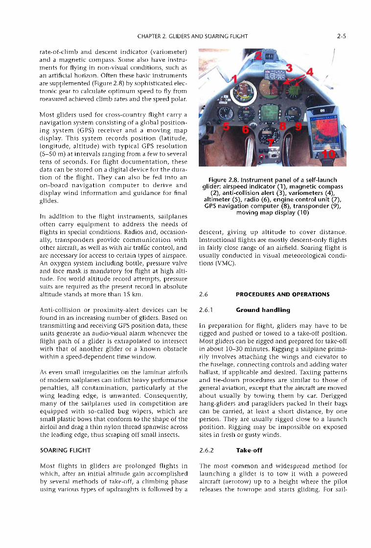
CHAPTER 2. GLIDERS AND SOARING FLIGHT 2-5
rate-of-climb and descent indicator (variometer)and a magnetic compass. Some also have instruments for flying in non-visual conditions, such asan artificial horizon. Often these basic instrumentsare supplemented (Figure 2.8) by sophisticated electronic gear to calculate optimum speed to fly frommeasured achieved climb rates and the speed polar.
Most gliders used for cross-country flight carry anavigation system consisting of a global positioning system (GPS) receiver and a moving mapdisplay. This system records position (latitude,longitude, altitude) with typical GPS resolution(5-50 m) at intervals ranging from a few to severaltens of seconds. For flight documentation, thesedata can be stored on a digital device for the duration of the flight. They can also be fed into anon-board navigation computer to derive anddisplay wind information and guidance for finalglides.
In addition to the flight instruments, sailplanesoften carry equipment to address the needs offlights in special conditions. Radios and, occasionally, transponders provide communication withother aircraft, as well as with air traffic control, andare necessary for access to certain types of airspace.An oxygen system including bottle, pressure valveand face mask is mandatory for flight at high altitude. For world altitude record attempts, pressuresuits are required as the present record in absolutealtitude stands at more than 15 km.
Anti-collision or proximity-alert devices can befound in an increasing number of gliders. Based ontransmitting and receiving GPS position data, theseunits generate an audio-visual alarm whenever theflight path of a glider is extrapolated to intersectwith that of another glider or a known obstaclewithin a speed-dependent time window.
As even small irregularities on the laminar airfoilsof modern sailplanes can inflict heavy performancepenalties, all contamination, particularly at thewing leading edge, is unwanted. Consequently,many of the sailplanes used in competition areequipped with so-called bug wipers, which aresmall plastic bows that conform to the shape of theairfoil and drag a thin nylon thread spanwise acrossthe leading edge, thus scraping off small insects.
Figure 2.8. Instrument panel of a self-launchglider: airspeed indicator (1), magnetic compass
(2), anti-collision alert (3), variometers (4),altimeter (5), radio (6), engine control unit (7),GPS navigation computer (8), transponder (9),
moving map display (10)
descent, giving up altitude to cover distance.Instructional flights are mostly descent-only flightsin fairly close range of an airfield. Soaring flight isusually conducted in visual meteorological conditions (VMC).
2.6 PROCEDURES AND OPERATIONS
2.6.1 Ground handling
In preparation for flight, gliders may have to berigged and pushed or towed to a take-off position.Most gliders can be rigged and prepared for take-offin about 10-30 minutes. Rigging a sailplane primarily involves attaching the wings and elevator tothe fuselage, connecting controls and adding waterballast, if applicable and desired. Taxiing patternsand tie-down procedures are similar to those ofgeneral aviation, except that the aircraft are movedabout usually by towing them by car. Deriggedhang-gliders and paragliders packed in their bagscan be carried, at least a short distance, by oneperson. They are usually rigged close to a launchposition. Rigging may be impossible on exposedsites in fresh or gusty winds.
SOARING FLIGHT 2.6.2 Take-off
Most flights in gliders are prolonged flights inwhich, after an initial altitude gain accomplishedby several methods of take-off, a climbing phaseusing various types of updraughts is followed by a
The most common and widespread method forlaunching a glider is to tow it with a poweredaircraft (aerotow) up to a height where the pilotreleases the towrope and starts gliding. For sail-
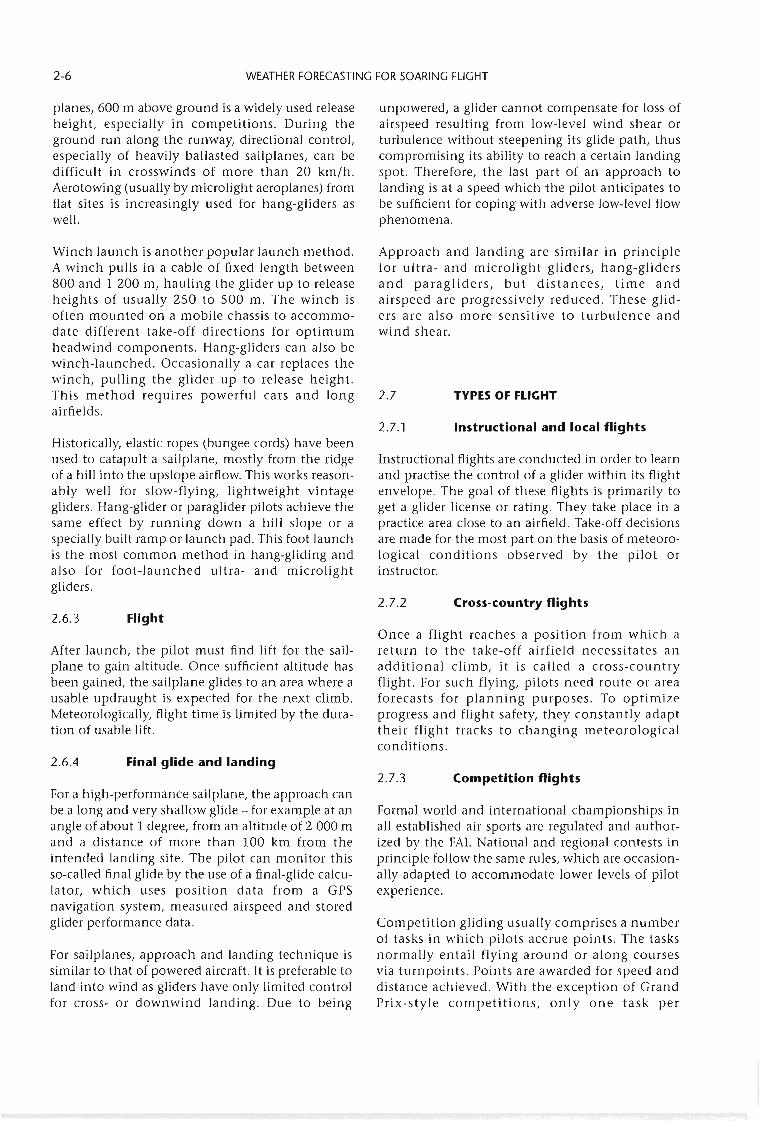
2-6 WEATHER FORECASTING FOR SOARING FLIGHT
planes, 600 m above ground is a Widely used releaseheight, especially in competitions. During theground run along the runway, directional control,especially of heavily ballasted sailplanes, can bedifficult in crosswinds of more than 20 km/h.Aerotowing (usually by microlight aeroplanes) fromflat sites is increasingly used for hang-gliders aswell.
Winch launch is another popular launch method.A winch pulls in a cable of fixed length between800 and 1 200 m, hauling the glider up to releaseheights of usually 250 to 500 m. The winch isoften mounted on a mobile chassis to accommodate different take-off directions for optimumheadwind components. Hang-gliders can also bewinch-launched. Occasionally a car replaces thewinch, pulling the glider up to release height.This method requires powerful cars and longairfields.
Historically, elastic ropes (bungee cords) have beenused to catapult a sailplane, mostly from the ridgeof a hill into the upslope airflow. This works reasonably well for slow-flying, lightweight vintagegliders. Hang-glider or paraglider pilots achieve thesame effect by running down a hill slope or aspecially built ramp or launch pad. This foot launchis the most common method in hang-gliding andalso for foot-launched ultra- and microlightgliders.
2.6.3 Flight
After launch, the pilot must find lift for the sailplane to gain altitude. Once sufficient altitude hasbeen gained, the sailplane glides to an area where ausable updraught is expected for the next climb.Meteorologically, flight time is limited by the duration of usable lift.
2.6.4 Final glide and landing
For a high-performance sailplane, the approach canbe a long and very shallow glide - for example at anangle of about 1 degree, from an altitude of 2 000 mand a distance of more than 100 km from theintended landing site. The pilot can monitor thisso-called final glide by the use of a final-glide calculator, which uses position data from a GPSnavigation system, measured airspeed and storedglider performance data.
For sailplanes, approach and landing technique issimilar to that of powered aircraft. It is preferable toland into wind as gliders have only limited controlfor cross- or downwind landing. Due to being
unpowered, a glider cannot compensate for loss ofairspeed resulting from low-level wind shear orturbulence without steepening its glide path, thuscompromising its ability to reach a certain landingspot. Therefore, the last part of an approach tolanding is at a speed which the pilot anticipates tobe sufficient for coping with adverse low-level flowphenomena.
Approach and landing are similar in principlefor ultra- and microlight gliders, hang-glidersand paragliders, but distances, time andairspeed are progressively reduced. These gliders are also more sensitive to turbulence andwind shear.
2.7 TYPES OF FLIGHT
2.7.1 Instructional and local flights
Instructional flights are conducted in order to learnand practise the control of a glider within its flightenvelope. The goal of these flights is primarily toget a glider license or rating. They take place in apractice area close to an airfield. Take-off decisionsare made for the most part on the basis of meteorological conditions observed by the pilot orinstructor.
2.7.2 Cross-country flights
Once a flight reaches a position from which areturn to the take-off airfield necessitates anadditional climb, it is called a cross-countryflight. For such flying, pilots need route or areaforecasts for planning purposes. To optimizeprogress and flight safety, they constantly adapttheir flight tracks to changing meteorologicalconditions.
2.7.3 Competition flights
Formal world and international championships inall established air sports are regulated and authorized by the FAI. National and regional contests inprinciple follow the same rules, which are occasionally adapted to accommodate lower levels of pilotexperience.
Competition gliding usually comprises a numberof tasks in which pilots accrue points. The tasksnormally entail flying around or along coursesvia turnpoints. Points are awarded for speed anddistance achieved. With the exception of GrandPrix-style competitions, only one task per

CHAPTER 2. GLIDERS AND SOARING FLIGHT 2-7
Record flights are individual efforts and often needpersonalized meteorological support. Successfulrecord attempts for speed, distance or altitude willmost likely make use of wave and, occasionally,convective updraughts. For the latter, atmosphericmotion is the major limiting factor (duration,strength and alignment of thermals). For waveflights, however, aerodynamic engineering becomesthe major limiting factor (maximum airspeed, flutter). Record attempts in wave lift require specializedmeteorological services, which might also have toaddress logistical and operational aspects of highaltitude flight.
competition class or group is set on a competition day.
Characteristic distance and time ranges for competition flying in sailplanes, hang-gliders andparagliders are related to the meteorological conditions. Usable altitudes are increasingly limited byairspace restrictions, and not necessarily by theheight ranges of updraughts. Cloud flying is usuallynot permitted in championships.
International sporting events are organized underthe rules of the FAI. The different competitions, theclasses (Table 2.2) and tasks are defined in the FAISporting Code (Table 2.4).
2.7.4 Record flights
Table 2.4. International gliding sporting events
FAI competitions Short description Tasks Meteorology
Sailplane Grand Prix Max. 20 pilots; one Speed tasks with "regatta Meteorological informationclass; duration 8 days; start" and a number of has to be prepared by the7-10 events/year in turnpoints, designated by organizer for the task-setterdifferent places all over the organizer and the pilotsthe world
Pilot's decision game onlyduring flight
Championships Up to 120 pilots in (a) Racing tasks; the Meteorological briefingdifferent FAI-c1asses organizer sets a number for the task-setter and the
World, continental, of turnpoints in a pilots by the organizernational, regional Open, 18 m, 15 m, sequence which the pilot
standard, world, club has to pass through The task-setter is able toand 20 m multi-seat select the type of task andclass (b) Assigned area task adjust it to the uncertainty
(AAT); (speed and of the weather situationdistance) the pilot has (for example, AAT whento achieve the highest showers or thunderstormsspeed and/or the greatest are expected)distance in an assignedarea, designated by the The pilot decides hisorganizer individual start time
and in An the distanceof his flight as well.Meteorological supportfrom a team meteorologistcan be helpful
Online contest OlC Cross-country flights Free selected turn points Meteorological flightare documented during flight as a polygon planning by the pilot
Classic and IGC-OlC worldwide on the before and during theworld league Internet and ranked Sprint task in a 2.5-hour flight
every day and every period with up to 3year, also special speed turnpointscompetitions for clubsof specified airfields
Barron Hilton Cup 2-year period; winners The longest triangular Meteorologically basedof 5 geographic flight in a region. The decision before the flightregions are invited to a course must be declaredsoaring week at Barron in advance by the pilotHilton's ranch

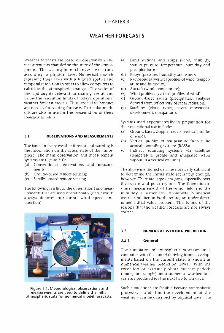
CHAPTER 3
WEATHER FORECASTS
The following is a list of the observations and measurements that are used operationally (here "wind"always denotes horizontal wind speed anddirection):
The basis for every weather forecast and warning isthe information on the actual state of the atmosphere. The main observation and measurementsystems are (Figure 3.1):(a) Conventional observations and measure
ments;(b) Ground-based remote sensing;(c) Satellite-based remote sensing.
Weather forecasts are based on observations andmeasurements that define the state of the atmosphere. The atmosphere changes over timeaccording to physical laws. Numerical modelsrepresent these laws with a limited spatial andtemporal resolution in order to allow computers tocalculate the atmospheric changes. The scales ofthe updraughts relevant to soaring are at andbelow the resolution limits of today's operationalweather forecast models. Thus, special techniquesare needed for soaring forecasts. Particular methods are also in use for the presentation of theseforecasts to pilots.
The simulation of atmospheric processes on acomputer, with the aim of deriving future developments based on the current state, is known asnumerical weather prediction (NWP). With theexception of extremely short forecast periods(hours, for example), most numerical weather forecasts are produced for the next two to ten days.
3.2.1 General
3.2 NUMERICAL WEATHER PREDICTION
(a) Land stations and ships (wind, visibility,station pressure, temperature, humidity andprecipitation);
(b) Buoys (pressure, humidity and wind);(c) Radiosondes (vertical profiles of wind, temper-
ature and humidity);(d) Aircraft (wind, temperature);(e) Wind profilers (vertical profiles of wind);(f) Ground-based radars (precipitation analyses
derived from reflectivity of radar radiation);(g) Satellites (cloud types, cover, movement,
development, dissipation).
The above-mentioned data are not nearly sufficientto determine the initial state accurately enough,however. There are large data gaps, especially overthe oceans and polar regions. The three-dimensional measurement of the wind field and thehumidity is particularly incomplete. Numericalweather prediction is, therefore, an under-determined initial value problem. This is one of thereasons that the weather forecasts are not alwayscorrect.
Systems used experimentally in preparation fortheir operational use include:(a) Ground-based Doppler radars (vertical profiles
of wind);(b) Vertical profiles of temperature from radio
acoustic sounding systems (RASS);(c) Indirect sounding systems via satellites
(temperature profile and integrated watervapour in a vertical column).
OBSERVATIONS AND MEASUREMENTS3.1
Figure 3.1. Meteorological observations andmeasurements are used to define the initial
atmospheric state for numerical model forecasts.
Such simulations are feasible because atmosphericprocesses - and thus the development of theweather - can be described by physical laws. The
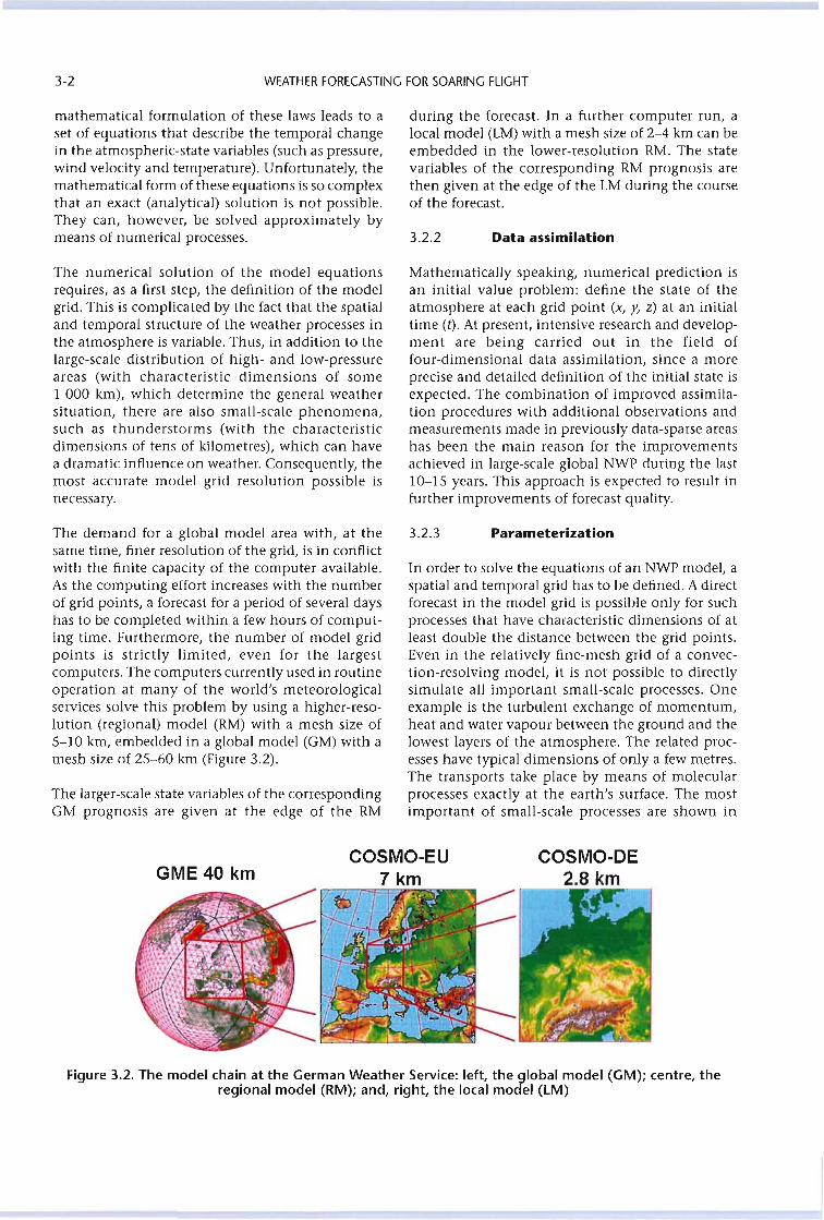
3-2 WEATHER FORECASTING FOR SOARING FLIGHT
mathematical formulation of these laws leads to aset of equations that describe the temporal changein the atmospheric-state variables (such as pressure,wind velocity and temperature). Unfortunately, themathematical form of these equations is so complexthat an exact (analytical) solution is not possible.They can, however, be solved approximately bymeans of numerical processes.
The numerical solution of the model equationsrequires, as a first step, the definition of the modelgrid. This is complicated by the fact that the spatialand temporal structure of the weather processes inthe atmosphere is variable. Thus, in addition to thelarge-scale distribution of high- and low-pressureareas (with characteristic dimensions of some1 000 km), which determine the general weathersituation, there are also small-scale phenomena,such as thunderstorms (with the characteristicdimensions of tens of kilometres), which can havea dramatic influence on weather. Consequently, themost accurate model grid resolution possible isnecessary.
The demand for a global model area with, at thesame time, finer resolution of the grid, is in conflictwith the finite capacity of the computer available.As the computing effort increases with the numberof grid points, a forecast for a period of several dayshas to be completed within a few hours of computing time. Furthermore, the number of model gridpoints is strictly limited, even for the largestcomputers. The computers currently used in routineoperation at many of the world's meteorologicalservices solve this problem by using a higher-resolution (regional) model (RM) with a mesh size of5-10 km, embedded in a global model (GM) with amesh size of 25-60 km (Figure 3.2).
The larger-scale state variables of the correspondingGM prognosis are given at the edge of the RM
during the forecast. In a further computer run, alocal model (LM) with a mesh size of 2-4 km can beembedded in the lower-resolution RM. The statevariables of the corresponding RM prognosis arethen given at the edge of the LM during the courseof the forecast.
3.2.2 Data assimilation
Mathematically speaking, numerical prediction isan initial value problem: define the state of theatmosphere at each grid point (x, y, z) at an initialtime (t). At present, intensive research and development are being carried out in the field offour-dimensional data assimilation, since a moreprecise and detailed definition of the initial state isexpected. The combination of improved assimilation procedures with additional observations andmeasurements made in previously data-sparse areashas been the main reason for the improvementsachieved in large-scale global NWP during the last10-15 years. This approach is expected to result infurther improvements of forecast quality.
3.2.3 Parameterization
In order to solve the equations of an NWP model, aspatial and temporal grid has to be defined. A directforecast in the model grid is possible only for suchprocesses that have characteristic dimensions of atleast double the distance between the grid points.Even in the relatively fine-mesh grid of a convection-resolving model, it is not possible to directlysimulate all important small-scale processes. Oneexample is the turbulent exchange of momentum,heat and water vapour between the ground and thelowest layers of the atmosphere. The related processes have typical dimensions of only a few metres.The transports take place by means of molecularprocesses exactly at the earth's surface. The mostimportant of small-scale processes are shown in
GME 40 kmCOSMO-EU
7 kmCOSMO-DE
2.8 kmn-----.
Figure 3.2. The model chain at the German Weather Service: left, the global model (GM); centre, theregional model (RM); and, right, the local model (lM)
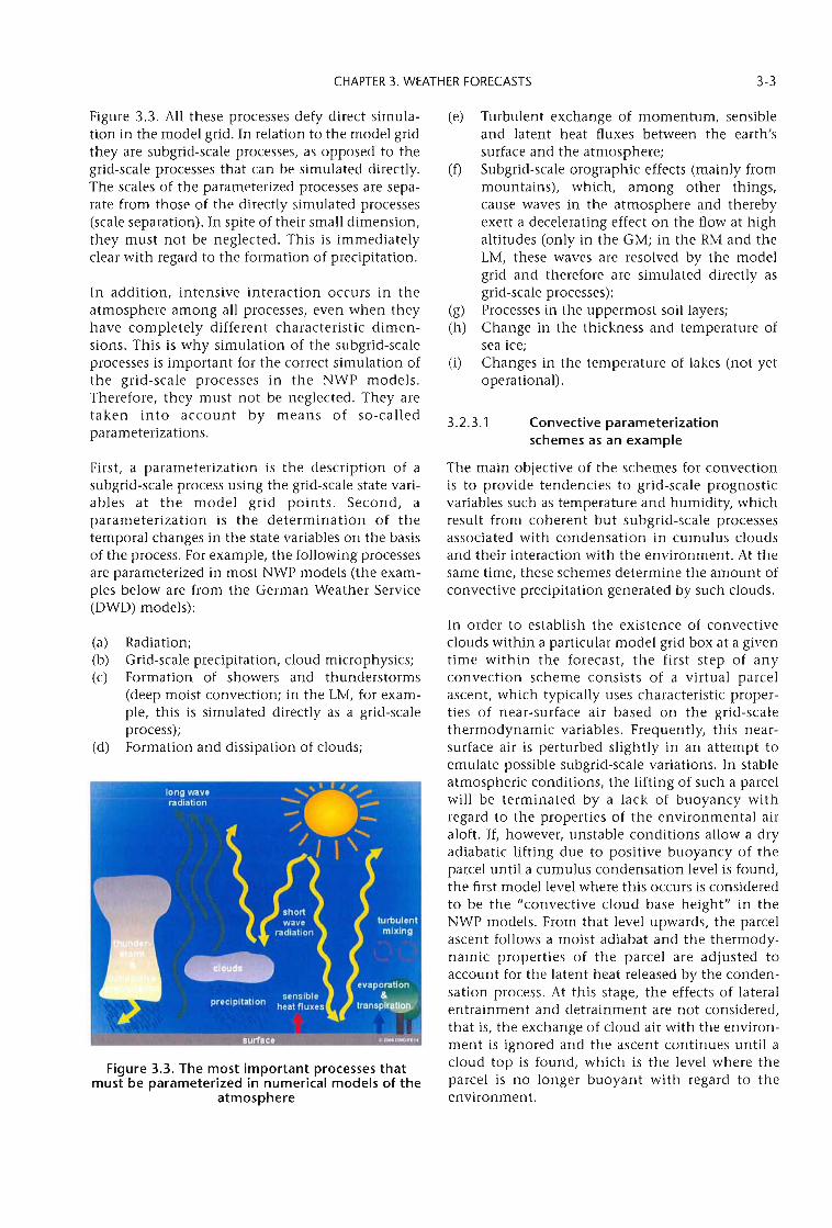
CHAPTER 3. WEATHER FORECASTS 3-3
3.2.3.1
Figure 3.3. All these processes defy direct simulation in the model grid. In relation to the model gridthey are subgrid-scale processes, as opposed to thegrid-scale processes that can be simulated directly.The scales of the parameterized processes are separate from those of the directly simulated processes(scale separation). In spite of their small dimension,they must not be neglected. This is immediatelyclear with regard to the formation of precipitation.
In addition, intensive interaction occurs in theatmosphere among all processes, even when theyhave completely different characteristic dimensions. This is why simulation of the subgrid-scaleprocesses is important for the correct simulation ofthe grid-scale processes in the NWP models.Therefore, they must not be neglected. They aretaken into account by means of so-calledparameterizations.
First, a parameterization is the description of asubgrid-scale process using the grid-scale state variables at the model grid points. Second, aparameterization is the determination of thetemporal changes in the state variables on the basisof the process. For example, the following processesare parameterized in most NWP models (the examples below are from the German Weather Service(DWD) models):
(a) Radiation;(b) Grid-scale precipitation, cloud microphysics;(c) Formation of showers and thunderstorms
(deep moist convection; in the LM, for example, this is simulated directly as a grid-scaleprocess);
(d) Formation and dissipation of clouds;
Figure 3.3. The most important processes thatmust be parameterized in numerical models of the
atmosphere
(e) Turbulent exchange of momentum, sensibleand latent heat fluxes between the earth'ssurface and the atmosphere;
(f) Subgrid-scale orographic effects (mainly frommountains), which, among other things,cause waves in the atmosphere and therebyexert a decelerating effect on the flow at highaltitudes (only in the GM; in the RM and theLM, these waves are resolved by the modelgrid and therefore are simulated directly asgrid-scale processes);
(g) Processes in the uppermost soil layers;(h) Change in the thickness and temperature of
sea ice;(i) Changes in the temperature of lakes (not yet
operational) .
Convective parameterizationschemes as an example
The main objective of the schemes for convectionis to proVide tendencies to grid-scale prognosticvariables such as temperature and humidity, whichresult from coherent but subgrid-scale processesassociated with condensation in cumulus cloudsand their interaction with the environment. At thesame time, these schemes determine the amount ofconvective precipitation generated by such clouds.
In order to establish the existence of convectiveclouds within a particular model grid box at a giventime within the forecast, the first step of anyconvection scheme consists of a virtual parcelascent, which typically uses characteristic properties of near-surface air based on the grid-scalethermodynamic variables. Frequently, this nearsurface air is perturbed slightly in an attempt toemulate possible subgrid-scale variations. In stableatmospheric conditions, the lifting of such a parcelwill be terminated by a lack of buoyancy withregard to the properties of the environmental airaloft. If, however, unstable conditions allow a dryadiabatic lifting due to positive buoyancy of theparcel until a cumulus condensation level is found,the first model level where this occurs is consideredto be the "convective cloud base height" in theNWP models. From that level upwards, the parcelascent follows a moist adiabat and the thermodynamic properties of the parcel are adjusted toaccount for the latent heat released by the condensation process. At this stage, the effects of lateralentrainment and detrainment are not considered,that is, the exchange of cloud air with the environment is ignored and the ascent continues until acloud top is found, which is the level where theparcel is no longer buoyant with regard to theenvironment.
3-4 WEATHER FORECASTING FOR SOARING FLIGHT
An important prerequisite for the correct formulation of parameterizations is the clear separation ofthe scale of the model from the scale of the parameterized process. The processes must be considerablysmaller, in spatial and temporal scales, than themodel grid scale (at least double the grid-point
The description of the topography of the earth'ssurface (external parameters) is closely related toparameterizations, and particularly to themodelling of the processes in the uppermost soillayers. Figure 3.4 shows the orography used in anLM. Steep slopes can be resolved more accurately(Figure 3.5).
unsatisfactory results, or if improved methods areoffered in literature, the existing methods are modified or replaced. The modification of an existingparameterization generally means an improveddefinition of free parameters that appear in themethod. Each change is followed by sophisticatedquality control of the new version within the forecast model as a whole. This entails calculatingforecasts with the modified model parallel to theoperational model over a period of one to twomonths. Then the results of both versions arecompared (verification) and both are comparedwith the actual weather. In the case of an overallpositive result, the previous operational model isreplaced by the modified model.
One of the most important differences between anRM and an LM is that the LM does not use a deepconvection parameterization. Instead, the LMresolves the larger parts of convection with itswhole life cycle, the generation of updraughts, thelatent heat release, the formation of ice particlesand the formation of a cold downdraught, whichcan generate gust fronts. Therefore, a better representation of convective gusts can be achieved. Thetravelling of such cells with the mean wind is simulated by the LM as well. A shallow convectionparameterization scheme may be reqUired for thesmaller scales of convection. Such a scheme cantransport moisture from the boundary layer to aheight of about 3 km, and it can therefore avoid theoverestimation of low cloud coverage. Without adeep convection parameterization, there seems tobe a need for a faster-sedimenting ice phase. Thus,a microphysics scheme can be extended by a newprecipitation class. The introduction of a detailedthree-dimensional turbulence scheme with a fulland more detailed soil model (Baldauf, 2004) couldbe a further improvement of the physicsparameterizations.
Scale separation3.2.3.2
The vertical profiles for updraught and downdraught mass flux are determined from thecloud-base mass flux and the lateral entrainmentand detrainment coefficients. Tendencies of thevarious thermodynamic model variables areobtained from the divergence of the respectivevertical fluxes computed on the basis of theupdraught and downdraught mass flux. The cloudcondensate content determined for the updraughtafter consideration of lateral and cloud top detrainment is converted to precipitation in deepconvective situations, but may evaporate partiallyor completely in the sub-cloud layer.
Since most NWP models employ a bulk mass-fluxconvection scheme, some determination of convective cloud type must be made in order to determineessential cloud properties, such as lateral entrainment coefficients. The cloud-base mass flux isderived from the total moisture convergence, thatis, the sum of surface evaporation and the horizontal convergence of moisture. The distinctionbetween shallow and deep convection is based onthe relative role of the surface evaporation and thehorizontal convergence of moisture. Alternativeapproaches, such as the approach used in the NWPmodel of the European Centre for Medium-RangeWeather Forecasts (ECMWF), determine the cloudbase mass flux for deep convection on the basis ofconvective available potential energy (CAPE) integrated over the cloud layers, and distinguishbetween various convection types mainly on thebasis of cloud thickness. Even though CAPE is notused directly in the parameterization schemesemployed by the NWP models of the DWD, it iscomputed and can be used as a diagnostic productthat carries information about the atmosphericstability simulated by the model. Once the cloudtype and associated properties are defined, theparcel ascent is repeated with due regard for theeffect of mixing through lateral entrainment anddetrainment on the cloud properties, and a revisedcloud top is determined.
The parameterizations contained in the modelsare constantly being monitored by verification ofthe forecast results. If this shows indications of
The parameterization scheme itself requires noexplicit determination of cloud cover at any modellevel. Convective clouds, just like other forms ofsubgrid-scale clouds, however, are an importantatmospheric constituent for the radiative transfercomputations in particular. A convective cloudfraction for each layer is diagnosed empiricallybased on the vertical extent of the convection, andit is proVided to model users.
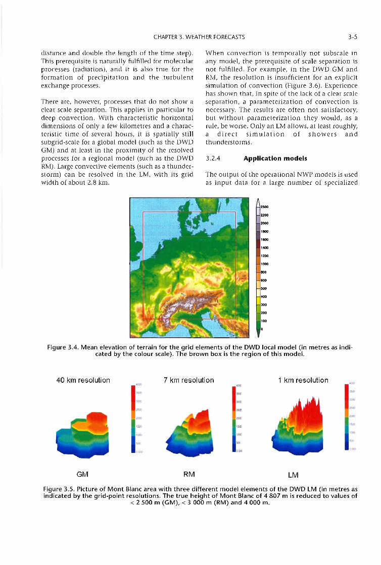
CHAPTER 3. WEATHER FORECASTS 3-5
distance and double the length of the time step).This prerequisite is naturally fulfilled for molecularprocesses (radiation), and it is also true for theformation of precipitation and the turbulentexchange processes.
There are, however, processes that do not show aclear scale separation. This applies in particular todeep convection. With characteristic horizontaldimensions of only a few kilometres and a characteristic time of several hours, it is spatially stillsubgrid-scale for a global model (such as the DWDGM) and at least in the proximity of the resolvedprocesses for a regional model (such as the DWDRM). Large convective elements (such as a thunderstorm) can be resolved in the LM, with its gridwidth of about 2.8 km.
When convection is temporally not subscale inany model, the prerequisite of scale separation isnot fulfilled. For example, in the DWD GM andRM, the resolution is insufficient for an explicitsimulation of convection (Figure 3.6). Experiencehas shown that, in spite of the lack of a clear scaleseparation, a parameterization of convection isnecessary. The results are often not satisfactory,but without parameterization they would, as arule, be worse. Only an LM allows, at least roughly,a direct simulation of showers andthunderstorms.
3.2.4 Application models
The output of the operational NWP models is usedas input data for a large number of specialized
~
2200
2000
1100
1100
1400
1200
1000
100
100
300
200
lOO
o
Figure 3.4. Mean elevation of terrain for the grid elements of the DWD local model (in metres as indicated by the colour scale). The brown box is the region of this model.
40 km resolution
GM
7 km resolution4000 «lOO
3"'" :l5OO
JOOC ....2<00 -2000 ll>lO
'''''' ,!CO
'000 IIXXl
500 !CO
000) 0"'"
RM
1 km resolution
LM
ISOD
1000
0000
Figure 3.5. Picture of Mont Blanc area with three different model elements of the DWD LM (in metres asindicated by the grid-point resolutions. The true height of Mont Blanc of 4 807 m is reduced to values of
< 2 500 m (GM), < 3 000 m (RM) and 4000 m.
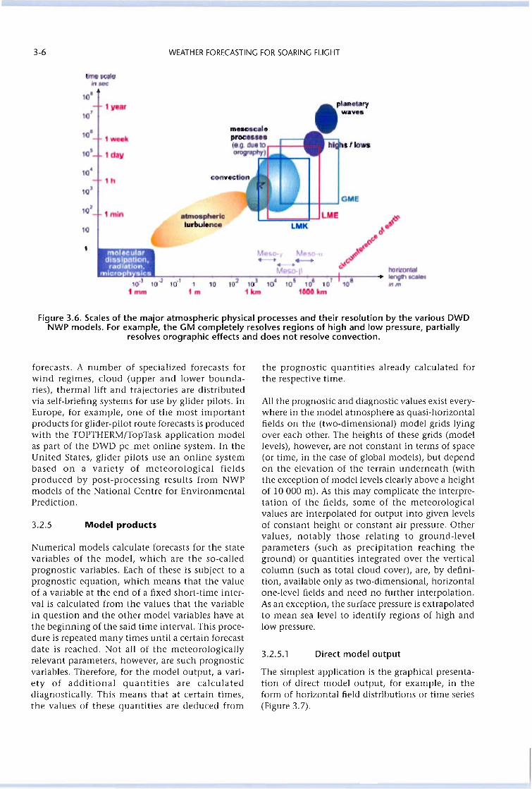
3-6
to
ftloleeul"rdlaslp6ltcm,radllltloll.
Inlcro h alea
WEATHER FORECASTING FOR SOARING FLIGHT
Figure 3.6. Scales of the major atmospheric physical processes and their resolution by the various DWDNWP models. For example, the GM completely resolves regions of high and low pressure, partially
resolves orographic effects and does not resolve convection.
the prognostic quantities already calculated forthe respective time.
The simplest application is the graphical presentation of direct model output, for example, in theform of horizontal field distributions or time series(Figure 3. 7) .
All the prognostic and diagnostic values exist everywhere in the model atmosphere as quasi-horizontalfields on the (two-dimensional) model grids lyingover each other. The heights of these grids (modellevels), however, are not constant in terms of space(or time, in the case of global models), but dependon the elevation of the terrain underneath (withthe exception of model levels clearly above a heightof 10 000 m). As this may complicate the interpretation of the fields, some of the meteorologicalvalues are interpolated for output into given levelsof constant height or constant air pressure. Othervalues, notably those relating to ground-levelparameters (such as precipitation reaching theground) or quantities integrated over the verticalcolumn (such as total cloud cover), are, by definition, available only as two-dimensional, horizontalone-level fields and need no further interpolation.As an exception, the surface pressure is extrapolatedto mean sea level to identify regions of high andlow pressure.
forecasts. A number of specialized forecasts forwind regimes, cloud (upper and lower boundaries), thermal lift and trajectories are distributedvia self-briefing systems for use by glider pilots. InEurope, for example, one of the most importantproducts for glider-pilot route forecasts is producedwith the TOPTHERM/TopTask application modelas part of the DWD pcmet online system. In theUnited States, glider pilots use an online systembased on a variety of meteorological fieldsproduced by post-processing results from NWPmodels of the National Centre for EnvironmentalPrediction.
3.2.5 Model products
Numerical models calculate forecasts for the statevariables of the model, which are the so-calledprognostic variables. Each of these is subject to aprognostic equation, which means that the valueof a variable at the end of a fixed short-time interval is calculated from the values that the variablein question and the other model variables have atthe beginning of the said time interval. This procedure is repeated many times until a certain forecastdate is reached. Not all of the meteorologicallyrelevant parameters, however, are such prognosticvariables. Therefore, for the model output, a variety of additional quantities are calculateddiagnostically. This means that at certain times,the values of these quantities are deduced from
3.2.5.1 Direct model output
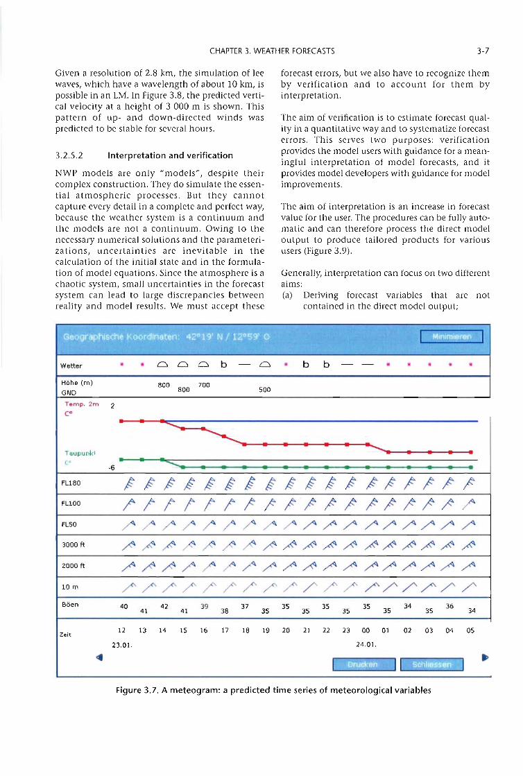
CHAPTER 3. WEATHER FORECASTS 3-7
Given a resolution of 2.8 km, the simulation of leewaves, which have a wavelength of about 10 km, ispossible in an LM. In Figure 3.8, the predicted vertical velocity at a height of 3 000 m is shown. Thispattern of up- and down-directed winds waspredicted to be stable for several hours.
NWP models are only "models", despite theircomplex construction. They do simulate the essential atmospheric processes. But they cannotcapture every detail in a complete and perfect way,because the weather system is a continuum andthe models are not a continuum. Owing to thenecessary numerical solutions and the parameterizations, uncertainties are inevitable in thecalculation of the initial state and in the formulation of model equations. Since the atmosphere is achaotic system, small uncertainties in the forecastsystem can lead to large discrepancies betweenreality and model results. We must accept these
3.2.5.2 Interpretation and verification
forecast errors, but we also have to recognize themby verification and to account for them byinterpretation.
The aim of verification is to estimate forecast quality in a quantitative way and to systematize forecasterrors. This serves two purposes: verificationproVides the model users with guidance for a meaningful interpretation of model forecasts, and itproVides model developers with guidance for modelimprovements.
The aim of interpretation is an increase in forecastvalue for the user. The procedures can be fully automatic and can therefore process the direct modeloutput to produce tailored products for varioususers (Figure 3.9).
Generally, interpretation can focus on two differentaims:(a) Deriving forecast variables that are not
contained in the direct model output;
.... ..~ I I; . ; • ; ~ [tJijOu1miJ."" ~
Wetter 0 0 0 b - 0 b b - -
Hohe (m) 800 700GND 800 500
Temp.2m 2CO
• • ""W~ • • • • • ~T8upunld • • • •
C' • • ~-6 • • • • • • • • • • • • • •FL180 t t ,$ ,t ,t t ~ t ,t ,t ,$ ,$ ~~;:;:;: ;:FL100 ~~ I I I I ;: ;: ?rrr rrrr~ ~
FLSO ~~~~~~~ ~,/\~~~~~~~
3000 ft ~~~~~~~~~~~~~~~~~~
2000 ft ,/\~~~~~~,/\~~~~~~~~~~
10 m ~~~/////~//~~~~~~~
Boen 40 42 39 37 35 35 35 34 3641 41 38 35 35 35 35 35 34
Zeit12 13 14 15 16 17 18 19 20 21 22 23 00 01 02 03 04 05
23.01. 24.01.
• •1 11 -ID 1.rlJl"~1 :lil .
Figure 3.7. A meteogram: a predicted time series of meteorological variables
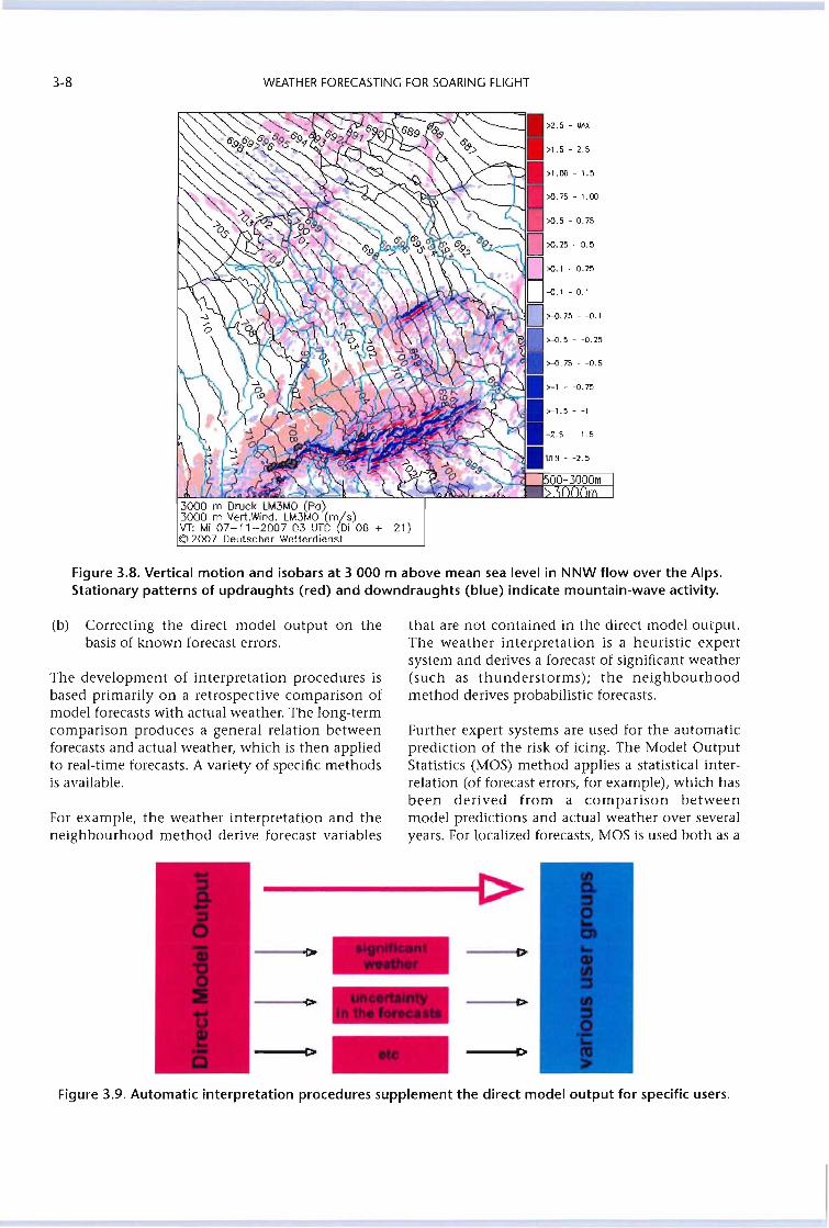
3-8 WEATHER FORECASTING FOR SOARING FLIGHT
3000 m Druck LM3MO (Po)3000 m VerLWind. LM3MO (m/s)VT: Mi 07-11-2007 03 UTC (Di 06 + 21)© 2007 Deutscher Wetterdienst
Figure 3.8. Vertical motion and isobars at 3 000 m above mean sea level in NNW flow over the Alps.Stationary patterns of updraughts (red) and downdraughts (blue) indicate mountain-wave activity.
(b) Correcting the direct model output on thebasis of known forecast errors.
The development of interpretation procedures isbased primarily on a retrospective comparison ofmodel forecasts with actual weather. The long-termcomparison produces a general relation betweenforecasts and actual weather, which is then appliedto real-time forecasts. A variety of specific methodsis available.
For example, the weather interpretation and theneighbourhood method derive forecast variables
that are not contained in the direct model output.The weather interpretation is a heuristic expertsystem and derives a forecast of significant weather(such as thunderstorms); the neighbourhoodmethod derives probabilistic forecasts.
Further expert systems are used for the automaticprediction of the risk of icing. The Model OutputStatistics (MOS) method applies a statistical interrelation (of forecast errors, for example), which hasbeen derived from a comparison betweenmodel predictions and actual weather over severalyears. For localized forecasts, MOS is used both as a
---I>
----~t>
----il>
---I>
Figure 3.9. Automatic interpretation procedures supplement the direct model output for specific users.
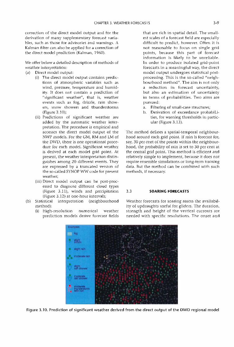
CHAPTER 3. WEATHER FORECASTS 3-9
correction of the direct model output and for thederivation of many supplementary forecast variables, such as those for advisories and warnings. AKalman filter can also be applied for a correction ofthe direct model prediction (Kalman, 1960).
We offer below a detailed description of methods ofweather interpretation:(a) Direct model output:
(i) The direct model output contains predictions of atmospheric variables such aswind, pressure, temperature and humidity. It does not contain a prediction of"significant weather", that is, weatherevents such as fog, drizzle, rain showers, snow showers and thunderstorms(Figure 3.10);
(ii) Predictions of significant weather areadded by the automatic weather interpretation. The procedure is empirical andaccesses the direct model output of theNWP models. For the GM, RM and LM ofthe DWD, there is one operational procedure for each model. Significant weatheris derived at each model grid point. Atpresent, the weather interpretation distinguishes among 20 different events. Theyare expressed by a truncated version ofthe so-called SYNOP WW code for presentweather;
(iii) Direct model output can be post-processed to diagnose different cloud types(Figure 3.11), winds and precipitation(Figure 3.12) at one-hour intervals;
(b) Statistical interpretation (neighbourhoodmethod):(i) High-resolution numerical weather
prediction models derive forecast fields
that are rich in spatial detail. The smallest scales of a forecast field are especiallydifficult to predict, however. Often it isnot reasonable to focus on single gridpoints, because this part of forecastinformation is likely to be unreliable.In order to produce isolated grid-pointforecasts in a meaningful way, the directmodel output undergoes statistical postprocessing. This is the so-called "neighbourhood method". The aim is not onlya reduction in forecast uncertainty,but also an estimation of uncertaintyin terms of probabilities. Two aims arepursued:a. Filtering of small-case structures;b. Derivation of exceedance probabiLi
ties, for warning thresholds in particular (Figure 3.13).
The method defines a spatial-temporal neighbourhood around each grid point. If rain is forecast for,say, 30 per cent of the points within the neighbourhood, the probability of rain is set to 30 per cent atthe central grid point. This method is efficient andrelatively simple to implement, because it does notrequire ensemble simulations or long-term trainingdata. But the method can be combined with suchmethods, if necessary.
3.3 SOARING FORECASTS
Weather forecasts for soaring assess the availability of updraughts useful for gliders. The duration,strength and height of the vertical currents areneeded with specific resolutions. The onset and
Figure 3.10. Prediction of significant weather derived from the direct output of the DWD regional model
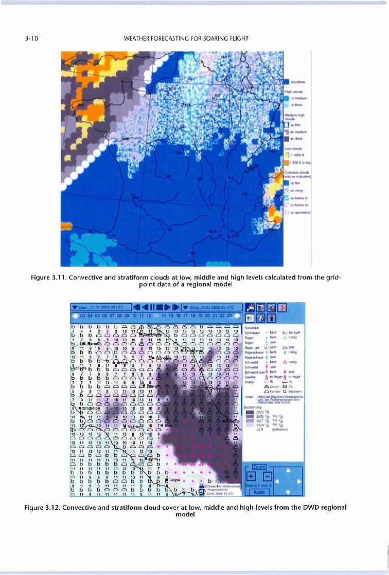
3-10 WEATHER FORECASTING FOR SOARING FLIGHT
!>is 7"bis '4blS",
_en""
Figure 3.11. Convective and stratiform clouds at low, middle and high levels calculated from the gridpoint data of a regional model
-~ • Ieitt IiUleittgatRegl3'l • IEdt .... n13I\g
RlgIn .:.-
RlIg<n gat r.u Iodt .-~ q Iodt • n8lil~,-Sd'ree61t • Is:tt ,,~__ v_~tlodt .-__ nm~R mHagel~ -9. ~k
t!:;OJ= BO>Cl OJtun b BIanrm
-t;-""""""~~.~
Bedecl<t.rog"_ ovc'"_ BKN'"_ SCT '4
FEW'"ClR
Figure 3.12. Convective and stratiform cloud cover at low, middle and high levels from the DWD regionalmodel
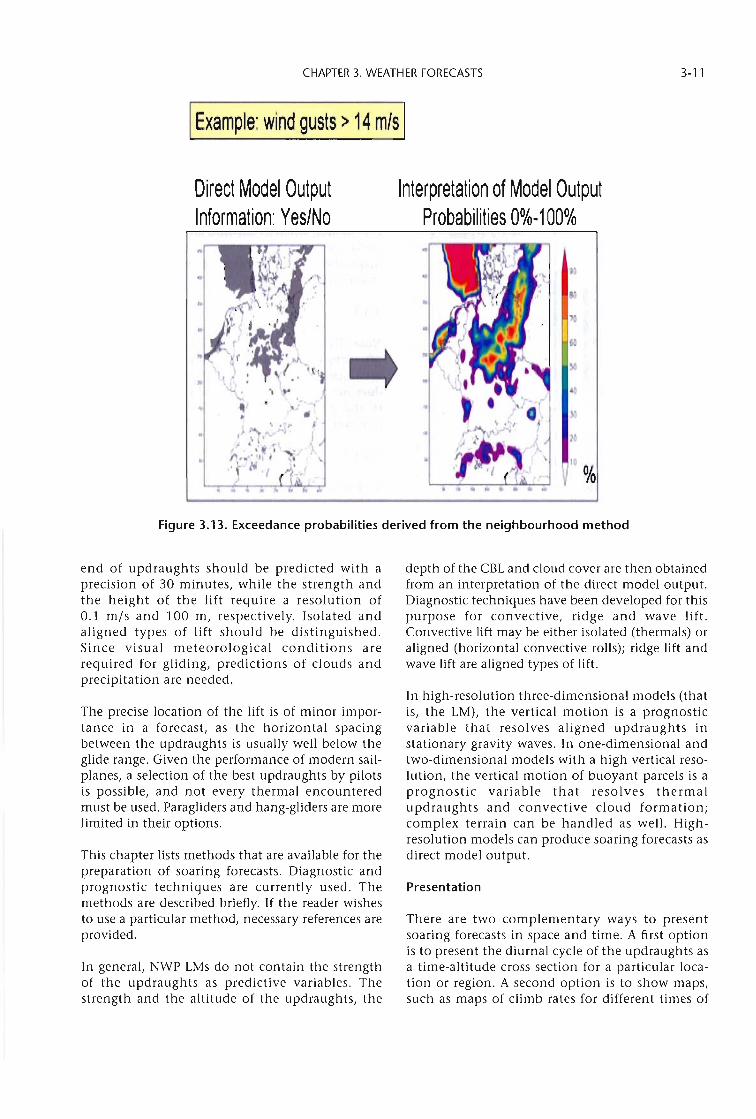
CHAPTER 3. WEATHER FORECASTS 3-11
xample: wind gusts> 14 m/s
Direct Model OutputInformation: Yes/No
Interpretation of Model OutputProbabilities 0%..100%
90
aD
70
60
~
40
~
~" :..i l:
\ J 20r
10 %
Figure 3.13. Exceedance probabilities derived from the neighbourhood method
end of updraughts should be predicted with aprecision of 30 minutes, while the strength andthe height of the lift require a resolution of0.1 m/s and 100 m, respectively. Isolated andaligned types of lift should be distinguished.Since visual meteorological conditions arerequired for gliding, predictions of clouds andprecipitation are needed.
The precise location of the lift is of minor importance in a forecast, as the horizontal spacingbetween the updraughts is usually well below theglide range. Given the performance of modern sailplanes, a selection of the best updraughts by pilotsis possible, and not every thermal encounteredmust be used. Paragliders and hang-gliders are morelimited in their options.
This chapter lists methods that are available for thepreparation of soaring forecasts. Diagnostic andprognostic techniques are currently used. Themethods are described briefly. If the reader wishesto use a particular method, necessary references areprovided.
In general, NWP LMs do not contain the strengthof the updraughts as predictive variables. Thestrength and the altitude of the updraughts, the
depth of the CBL and cloud cover are then obtainedfrom an interpretation of the direct model output.Diagnostic techniques have been developed for thispurpose for convective, ridge and wave lift.Convective lift may be either isolated (thermals) oraligned (horizontal convective rolls); ridge lift andwave lift are aligned types of lift.
In high-resolution three-dimensional models (thatis, the LM), the vertical motion is a prognosticvariable that resolves aligned updraughts instationary gravity waves. In one-dimensional andtwo-dimensional models with a high vertical resolution, the vertical motion of buoyant parcels is aprognostic variable that resolves thermalupdraughts and convective cloud formation;complex terrain can be handled as well. Highresolution models can produce soaring forecasts asdirect model output.
Presentation
There are two complementary ways to presentsoaring forecasts in space and time. A first optionis to present the diurnal cycle of the updraughts asa time-altitude cross section for a particular location or region. A second option is to show maps,such as maps of climb rates for different times of
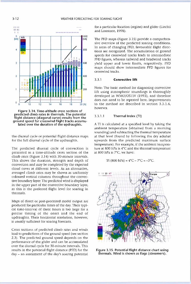
3-12 WEATHER FORECASTING FOR SOARING FLIGHT
cs ccliS lICS C
for a particular location (region) and glider (Liechtiand Lorenzen, 1998).
the diurnal cycle or potential flight distance mapsfor the full diurnal cycle of the updraughts.
Figure 3.14. Time-altitude cross sections ofpredicted climb rates in thermals. The potentialflight distance (diagonal curve) results from the
ground speed for crosswind flight tracks accumu-lated over the duration of the updraughts.
Maps of direct or post-processed model output areproduced for particular times of the day. Their typical time-interval of three hours is too large for aprecise timing of the onset and the end ofupdraughts. Their horizontal resolution, however,is usually sufficient for soaring forecasts.
Thermal Index (TI)3.3.1.1
3.3.1 Convective lift
Note: The basic method for diagnosing convectivelift using atmospheric soundings is thoroughlydeveloped in WMO/OSTIV (1993), and thereforedoes not need to be repeated here. Improvementsto the method are described in section 3.3.1.6,however.
The PFD maps (Figure 3.15) provide a comprehensive overview of the predicted soaring conditions.In areas of changing PFD, favourable flight directions are recognized. The accumulation of groundspeeds for crosswind tracks leads to intermediatePFD figures, whereas tailwind and headwind tracksyield upper and lower limits, respectively. PFDmaps should show intermediate PFD figures forcrosswind tracks.
Figure 3.15. Potential flight distance chart usingthermals. Wind is shown as flags (streamers).
TI (800 hPa) = 4°C - rc =-3°C.
A TI is calculated at a specified level by taking theambient temperature (obtained from a morningsounding) and subtracting the thermal temperatureat that level (found by follOWing the dry adiabatupwards from the predicted maximum surfacetemperature). For example, if the ambient temperature at 800 hPa is 4°C and the thermal temperatureat 800 hPa is rc, we have:
00
000km)
200
600
BOO
20 [hI1816141210
i1[
/0+
/1111
-1_111 1 l
4
,)- r--, ..
1.1
.Y/1
3
4
2
o 8
5[km)
The predicted diurnal cycle of convection ispresented as a time-altitude cross section of theclimb rates (Figure 3.14) with 30-minute intervals.This shows the duration, strength and depth ofconvection and may be completed by the expectedcloud cover at different levels. As an alternative,averaged climb rates may be shown as uniformlycoloured vertical columns throughout the convective boundary layer. The predicted wind is displayedin the upper part of the convective boundary layer,as this is the preferred flight level for soaring inthermals.
Cross sections of predicted climb rates and windslead to predictions of the ground speed (see section2.3). The predicted ground speed depends on theperformance of the glider and can be accumulatedover the diurnal cycle for 30-minute intervals. Thisresults in the potential flight distance (PFD) for theday - an assessment of the day's soaring potential
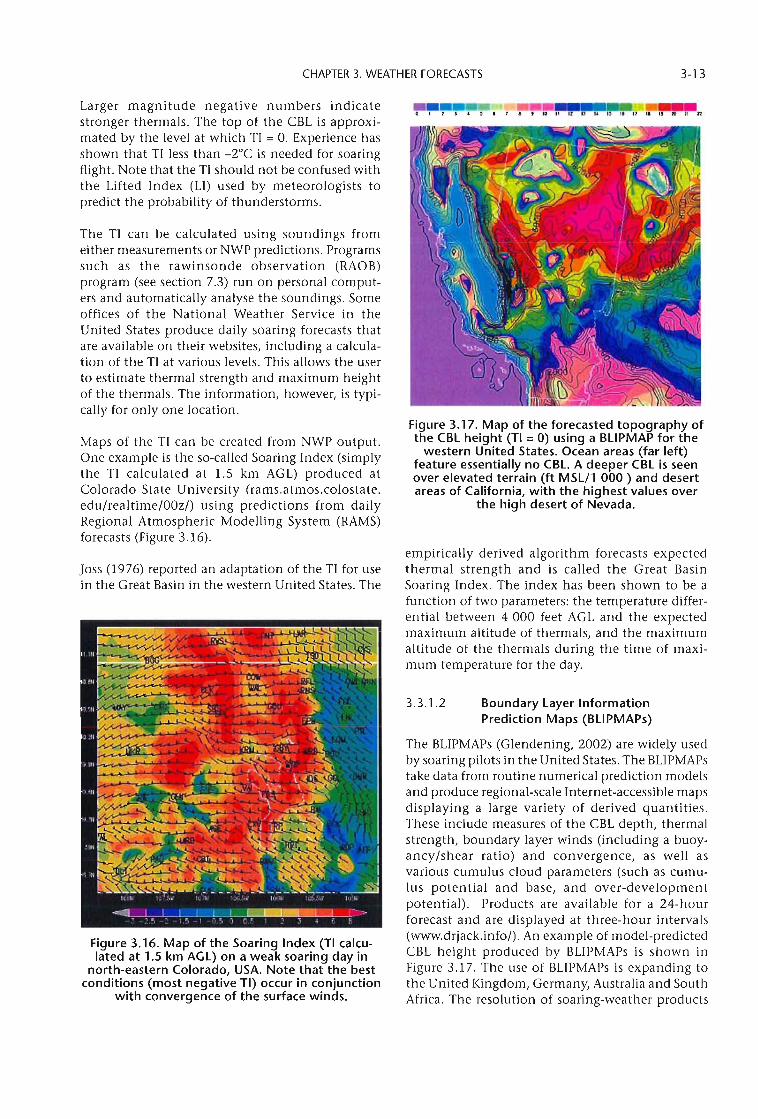
CHAPTER 3. WEATHER FORECASTS 3-13
Figure 3.17. Map of the forecasted topography ofthe CBl height (TI =0) using a BlIPMAP for the
western United States. Ocean areas (far left)feature essentially no CBl. A deeper CBl is seenover elevated terrain (ft MSl/l 000 ) and desertareas of California, with the highest values over
the high desert of Nevada.
empirically derived algorithm forecasts expectedthermal strength and is called the Great BasinSoaring Index. The index has been shown to be afunction of two parameters: the temperature differential between 4000 feet AGL and the expectedmaximum altitude of thermals, and the maximumaltitude of the thermals during the time of maximum temperature for the day.
l' 17 I1U IS---=:::='.-t I 1 J C 5 • 1 I , III 11 1% D
Boundary layer InformationPrediction Maps (BlIPMAPs)
The BLlPMAPs (Glendening, 2002) are Widely usedby soaring pilots in the United States. The BLlPMAPstake data from routine numerical prediction modelsand produce regional-scale Internet-accessible mapsdisplaying a large variety of derived quantities.These include measures of the CBL depth, thermalstrength, boundary layer winds (including a buoyancy/shear ratio) and convergence, as well asvarious cumulus cloud parameters (such as cumulus potential and base, and over-developmentpotential). Products are available for a 24-hourforecast and are displayed at three-hour intervals(www.drjack.info/). An example of model-predictedCBL height produced by BLlPMAPs is shown inFigure 3.17. The use of BLlPMAPs is expanding tothe United Kingdom, Germany, Australia and SouthAfrica. The resolution of soaring-weather products
3.3.1.2
Figure 3.16. Map of the Soaring Index (TI calculated at 1.5 km AGl) on a weak soaring day in
north-eastern Colorado, USA. Note that the bestconditions (most negative TI) occur in conjunction
with convergence of the surface winds.
Maps of the TI can be created from NWP output.One example is the so-called Soaring Index (simplythe TI calculated at l.S km AGL) produced atColorado State University (rams.atmos.colostate.edu/realtime/OOzl) using predictions from dailyRegional Atmospheric Modelling System (RAMS)forecasts (Figure 3.16).
The TI can be calculated using soundings fromeither measurements or NWP predictions. Programssuch as the rawinsonde observation (RAOB)program (see section 7.3) run on personal computers and automatically analyse the soundings. Someoffices of the National Weather Service in theUnited States produce daily soaring forecasts thatare available on their websites, including a calculation of the TI at various levels. This allows the userto estimate thermal strength and maximum heightof the thermals. The information, however, is typically for only one location.
Larger magnitude negative numbers indicatestronger thermals. The top of the CBL is approximated by the level at which TI = O. Experience hasshown that TI less than _2°C is needed for soaringflight. Note that the TI should not be confused withthe Lifted Index (Ll) used by meteorologists topredict the probability of thunderstorms.
joss (1976) reported an adaptation of the TI for usein the Great Basin in the western United States. The
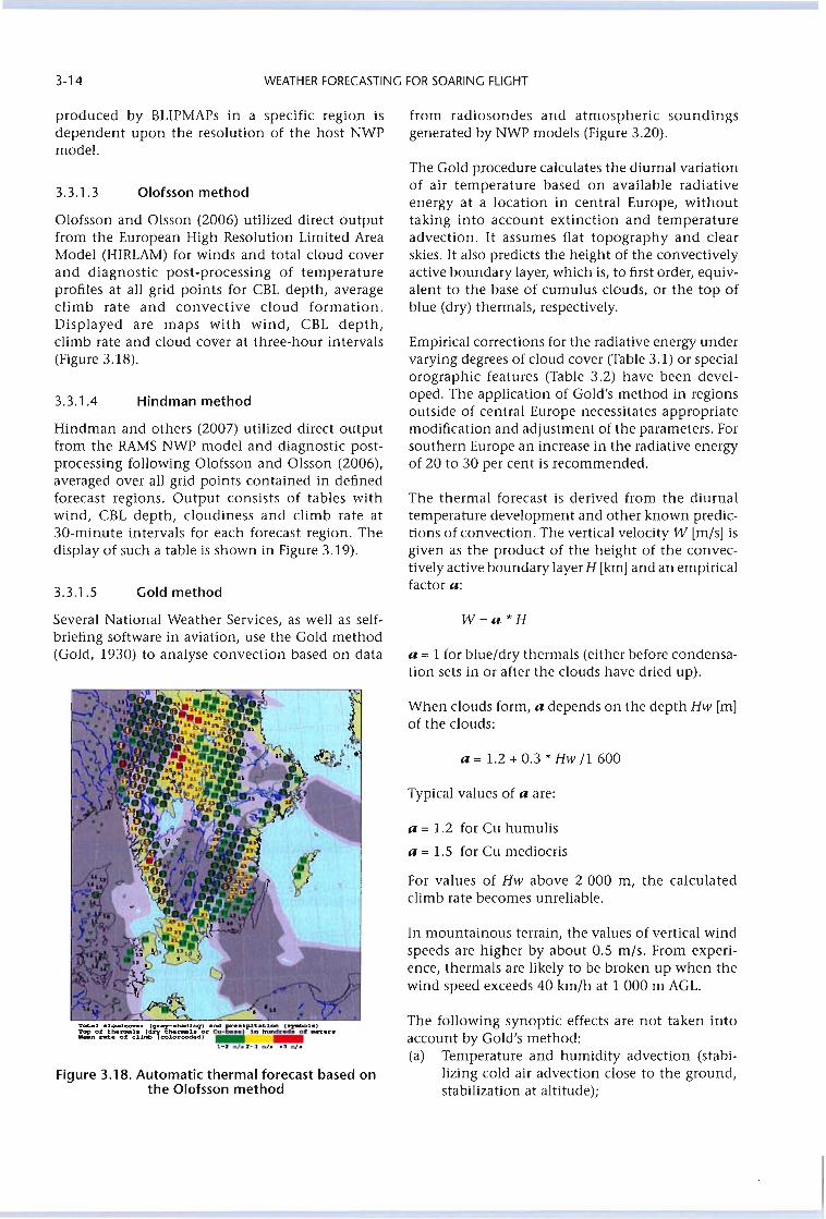
3-14 WEATHER FORECASTING FOR SOARING FLIGHT
produced by BLIPMAPs in a specific region isdependent upon the resolution of the host NWPmodel.
from radiosondes and atmospheric soundingsgenerated by NWP models (Figure 3.20).
Hindman and others (2007) utilized direct outputfrom the RAMS NWP model and diagnostic postprocessing following Olofsson and Olsson (2006),averaged over all grid points contained in definedforecast regions. Output consists of tables withwind, CBL depth, cloudiness and climb rate at30-minute intervals for each forecast region. Thedisplay of such a table is shown in Figure 3.19).
Olofsson and Olsson (2006) utilized direct outputfrom the European High Resolution Limited AreaModel (HIRLAM) for winds and total cloud coverand diagnostic post-processing of temperatureprofiles at all grid points for CBL depth, averageclimb rate and convective cloud formation.Displayed are maps with wind, CBL depth,climb rate and cloud cover at three-hour intervals(Figure 3.18).
3.3.1.3
3.3.1.4
3.3.1.5
Olofsson method
Hindman method
Gold method
The Gold procedure calculates the diurnal variationof air temperature based on available radiativeenergy at a location in central Europe, withouttaking into account extinction and temperatureadvection. It assumes flat topography and clearskies. It also predicts the height of the convectivelyactive boundary layer, which is, to first order, equivalent to the base of cumulus clouds, or the top ofblue (dry) thermals, respectively.
Empirical corrections for the radiative energy undervarying degrees of cloud cover (Table 3.1) or specialorographic features (Table 3.2) have been developed. The application of Gold's method in regionsoutside of central Europe necessitates appropriatemodification and adjustment of the parameters. Forsouthern Europe an increase in the radiative energyof 20 to 30 per cent is recommended.
The thermal forecast is derived from the diurnaltemperature development and other known predictions of convection. The vertical velocity W [m/s] isgiven as the product of the height of the convectively active boundary layer H [km] and an empiricalfactor a:
Several National Weather Services, as well as selfbriefing software in aviation, use the Gold method(Gold, 1930) to analyse convection based on data
~.1 c.1oud-.r IfjJlE"~-.haod.u.q1 aftd pC'.clpJ.cat.lon C.,--bOl_,~o~:-~;J:~~~~IIE"cu-bII_r J.n hundliiiiiit: .-ten
1-2 -.1.2-3 -./...3-'/.
Figure 3.18. Automatic thermal forecast based onthe Olofsson method
W=a *H
a = 1 for blue/dry thermals (either before condensation sets in or after the clouds have dried up).
When clouds form, a depends on the depth Hw [m]of the clouds:
a = 1.2 + 0.3 * Hw /1 600
Typical values of a are:
a = 1.2 for Cu humulis
a = 1.5 for Cu mediocris
For values of Hw above 2 000 m, the calculatedclimb rate becomes unreliable.
In mountainous terrain, the values of vertical windspeeds are higher by about 0.5 m/so From experience, thermals are likely to be broken up when thewind speed exceeds 40 km/h at 1 000 m AGL.
The following synoptic effects are not taken intoaccount by Gold's method:(a) Temperature and humidity advection (stabi
lizing cold air advection close to the ground,stabilization at altitude);
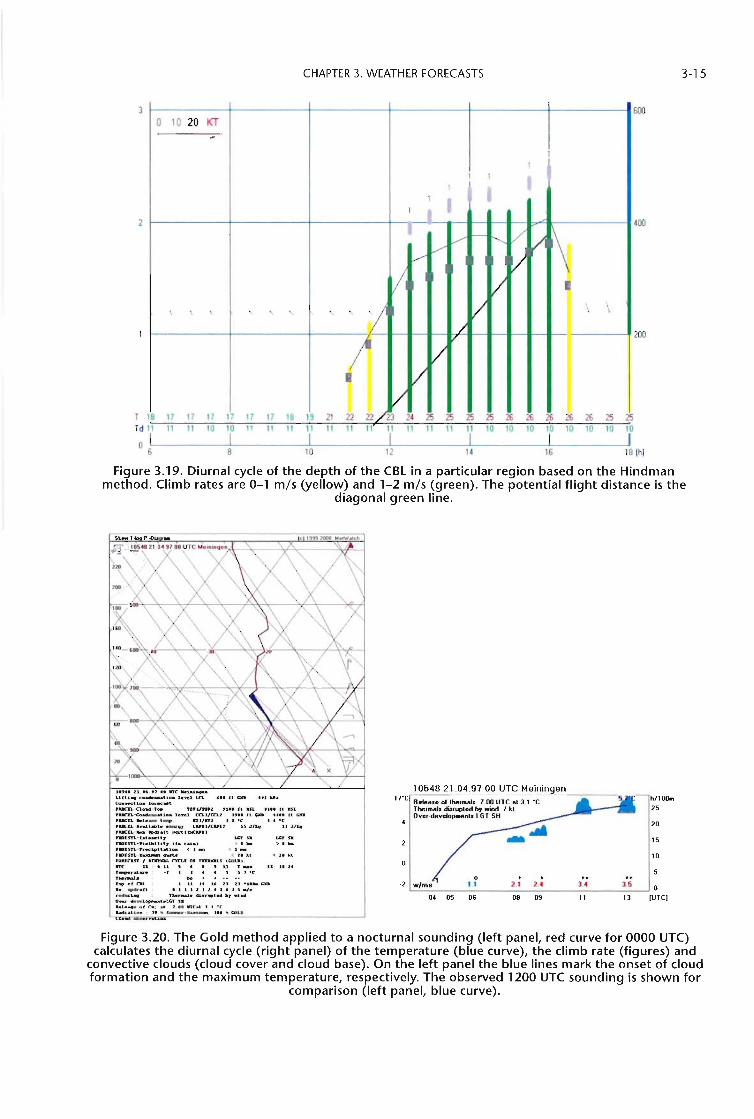
CHAPTER 3. WEATHER FORECASTS 3-15
200
600
400
o 10 20 KT
-1
11 1 I1 I
1 ~ I11
...-/ - I"--- / /1 !\.......... VV
I~ V\ \ \ , , , , , '/ / \ \
/
I VI /
V18 17 17 17 17 17 17 18 19 21 22 22/23 24 ~ ~ ~ ~ ~ ~ ~ ~ ~ ~ ~
3
TTdl1 111110101111 t1 11 11 11 11 111111 11111010101010101010
o I I I I I I I6 8 10 12 14 16 18 (hI
Figure 3.19. Diurnal cycle of the depth of the CBl in a particular region based on the Hindmanmethod. Climb rates are 0-1 m/s (yellow) and 1-2 m/s (green). The potential flight distance is the
diagonal green line.
hJl0o..25
20
15
10
.. ..).4 3.5 011 1) IUTC)08 ~
o ••1 1 2. T 2.4
05 06
rl_0_6_48_2_1._0_4_.9_7_0_0_U_T-...:C_M_e.:...i_ni_nLge.:...n_--:::-__Trc R_Ie••_ 0111"" ...1. 1.00 UTC .t 3.1 'C
The,MS diSlupted bJ wind I kIOver·developmentl LGT SH
US4. 21. .... '7 .. ne Md.....,..LJ..u.... c....-.... L•• '.-.1 L(1 U. 1\ ~ IU ...c.."I"M:'t-I_ t.rec:..t.'&aCIl.-a••-T.. TO'l/'fO.' 'u. n ItS1. ,u. It IISI.,aacn.-eo.....,-..,u••••~ a:Ll/CCLI u .. ft ~ ...... n IiiIO
.aaca~ ..1._ t.... nl/n, .'·C I .. 'C'UCKL In.U l. --nu canl/CUu n .JIE4 11 J/E4.aacn.·lIouI- n ...... I~aJ~~-~~t7 ~n ~u
~STL·'·:... u.U_it7 u. rai.a. ) • .. ) ...rmAsn.·Pr.c~IUt.I_ < I _ < I _
"'DIIsn.-~ w-t-- < " ...nlaK"an I • .-...u. cn:u: .1' TUUaaLS eCDU Inc n. C.U 5 .. I , U 1' __1'....r~_ ., ...... ') ".e,.~ be ••••••
..... t OL 1 U 14 U U lJ 'U_ CIlII
..........n . • • 1 • , I , ...... ') .-./•
....t.ri... n......... ~t.. ~Twi..o-r·...-:a .........LCT nkI._ ., c.:.t .,... nc.t • I 'Ca.a.u.U__ - 'n ... S-,r-~ 11'''' COU
Figure 3.20. The Gold method applied to a nocturnal sounding (left panel, red curve for 0000 UTC)calculates the diurnal cycle (right panel) of the temperature (blue curve), the climb rate (figures) and
convective clouds (cloud cover and cloud base). On the left panel the blue lines mark the onset of cloudformation and the maximum temperature, respectively. The observed 1200 UTC sounding is shown for
comparison (left panel, blue curve).
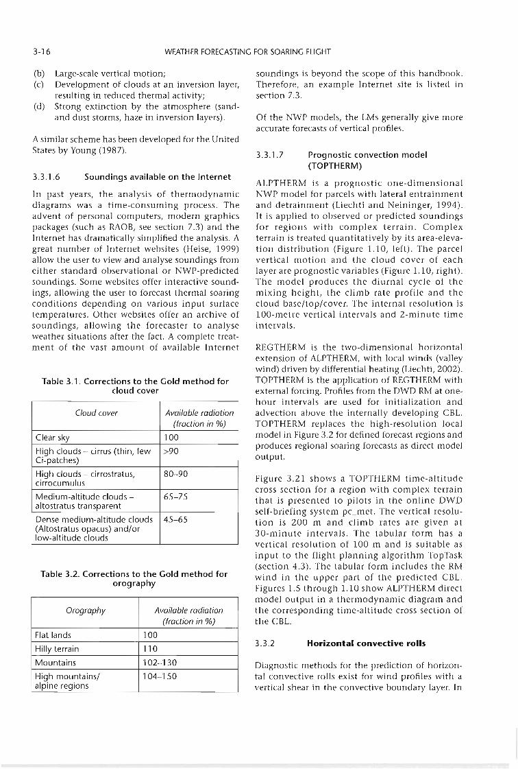
3-16 WEATHER FORECASTING FOR SOARING FLIGHT
Table 3.1. Corrections to the Gold method forcloud cover
Table 3.2. Corrections to the Gold method fororography
A similar scheme has been developed for the UnitedStates by Young (1987).
(b) Large-scale vertical motion;(c) Development of clouds at an inversion layer,
resulting in reduced thermal activity;(d) Strong extinction by the atmosphere (sand
and dust storms, haze in inversion layers).
Prognostic convection model(TOPTHERM)
3.3.1.7
REGTHERM is the two-dimensional horizontalextension of ALPTHERM, with local winds (valleywind) driven by differential heating (Liechti, 2002).TOPTHERM is the application of REGTHERM withexternal forcing. Profiles from the DWD RM at onehour intervals are used for initialization andadvection above the internally developing CBL.TOPTHERM replaces the high-resolution localmodel in Figure 3.2 for defined forecast regions andproduces regional soaring forecasts as direct modeloutput.
ALPTHERM is a prognostic one-dimensionalNWP model for parcels with lateral entrainmentand detrainment (Liechti and Neininger, 1994).It is applied to observed or predicted soundingsfor regions with complex terrain. Complexterrain is treated quantitatively by its area-elevation distribution (Figure 1.10, left). The parcelvertical motion and the cloud cover of eachlayer are prognostic variables (Figure 1.10, right).The model produces the diurnal cycle of themixing height, the climb rate profile and thecloud base/top/cover. The internal resolution islOO-metre vertical intervals and 2-minute timeintervals.
3.3.2 Horizontal convective rolls
soundings is beyond the scope of this handbook.Therefore, an example Internet site is listed insection 7.3.
Figure 3.21 shows a TOPTHERM time-altitudecross section for a region with complex terrainthat is presented to pilots in the online DWDself-briefing system pc_met. The vertical resolution is 200 m and climb rates are given at30-minute intervals. The tabular form has avertical resolution of 100 m and is suitable asinput to the flight planning algorithm TopTask(section 4.3). The tabular form includes the RMwind in the upper part of the predicted CBL.Figures 1.S through 1.10 show ALPTHERM directmodel output in a thermodynamic diagram andthe corresponding time-altitude cross section ofthe CBL.
Of the NWP models, the LMs generally give moreaccurate forecasts of vertical profiles.
Diagnostic methods for the prediction of horizontal convective rolls exist for wind profiles with avertical shear in the convective boundary layer. In
Soundings available on the Internet3.3.1.6
In past years, the analysis of thermodynamicdiagrams was a time-consuming process. Theadvent of personal computers, modern graphicspackages (such as RAOB, see section 7.3) and theInternet has dramatically simplified the analysis. Agreat number of Internet websites (Heise, 1999)allow the user to view and analyse soundings fromeither standard observational or NWP-predictedsoundings. Some websites offer interactive soundings, allowing the user to forecast thermal soaringconditions depending on various input surfacetemperatures. Other websites offer an archive ofsoundings, allowing the forecaster to analyseweather situations after the fact. A complete treatment of the vast amount of available Internet
Cloud cover Available radiation(fraction in %)
Clear sky 100
High clouds - cirrus (thin, few >90Ci-patches)
High clouds - cirrostratus, 80-90cirrocumulus
Medium-altitude clouds - 65-75altostratus transparent
Dense medium-altitude clouds 45-65(Altostratus opacus) and/orlow-altitude clouds
Orography Available radiation(fraction in %)
Flat lands 100
Hilly terrain 110
Mountains 102-130
High mountains/ 104-150alpine regions
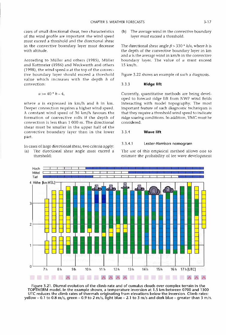
CHAPTER 3. WEATHER FORECASTS 3-17
cases of small directional shear, two characteristicsof the wind profile are important: the wind speedmust exceed a threshold and the directional shearin the convective boundary layer must decreasewith altitude.
According to Muller and others (1985), Mullerand Kottmeier (1986) and Weckwerth and others(1998), the wind speed u at the top of the convective boundary layer should exceed a thresholdvalue which increases with the depth h ofconvection:
(b) The average wind in the convective boundarylayer must exceed a threshold.
The directional shear angle fJ > 330 * h/u, where h isthe depth of the convective boundary layer in kmand u is the average wind in km/h in the convectiveboundary layer. The value of u must exceed15 km/h.
Figure 3.22 shows an example of such a diagnosis.
3.3.3 Ridge lift
Currently, quantitative methods are being developed to forecast ridge lift from NWP wind fieldsinteracting with model topography. The mostimportant feature of such diagnostic techniques isthat they require a threshold wind speed to indicateridge soaring conditions. In addition, VMC must beconsidered.
The use of this empirical method allows one toestimate the probability of lee wave development
U >= 40 * h - 4,
where u is expressed in km/h and h in km.Deeper convection requires a higher wind speed.A constant wind speed of 36 km/h favours theformation of convective rolls if the depth ofconvection is less than 1 000 m. The directionalshear must be smaller in the upper half of theconvective boundary layer than in the lowerpart.
In cases of large directional shear, two criteria apply:(a) The directional shear angle must exceed a
threshold;
3.3.4
3.3.4.1
Wave lift
lester-Harrison nomogram
HochMittelTiel
4 Hohe [km MSLI-,.----,.----,---,---,--;=;-,---,---,---,---.--.-----,
3 I---+--+-i-If-+-+-
2 I---+--+-i-If-+-+-i-If-
OL.-_---JL.-_---JL.-_---JL....-_---l__---l__---l__---l__--l__--l__--l__--l__-J
7h 8h 9h 10 h 11 h 12 h
A .JIJ
13 h 14 h 15 h 16 h 17 h lUTe]
J\l
Figure 3.21. Diurnal evolution of the climb rate and of cumulus clouds over complex terrain in theTOPTHERM model. In the example shown, a temperature inversion at 1.5 km between 0700 and 1300UTC reduces the climb rates of thermals originating from elevations below the inversion. Climb rates:
yellow - 0.1 to 0.8 m/Sf green - 0.9 to 2 m/Sf light blue - 2.1 to 3 m/s and dark blue - greater than 3 m/so
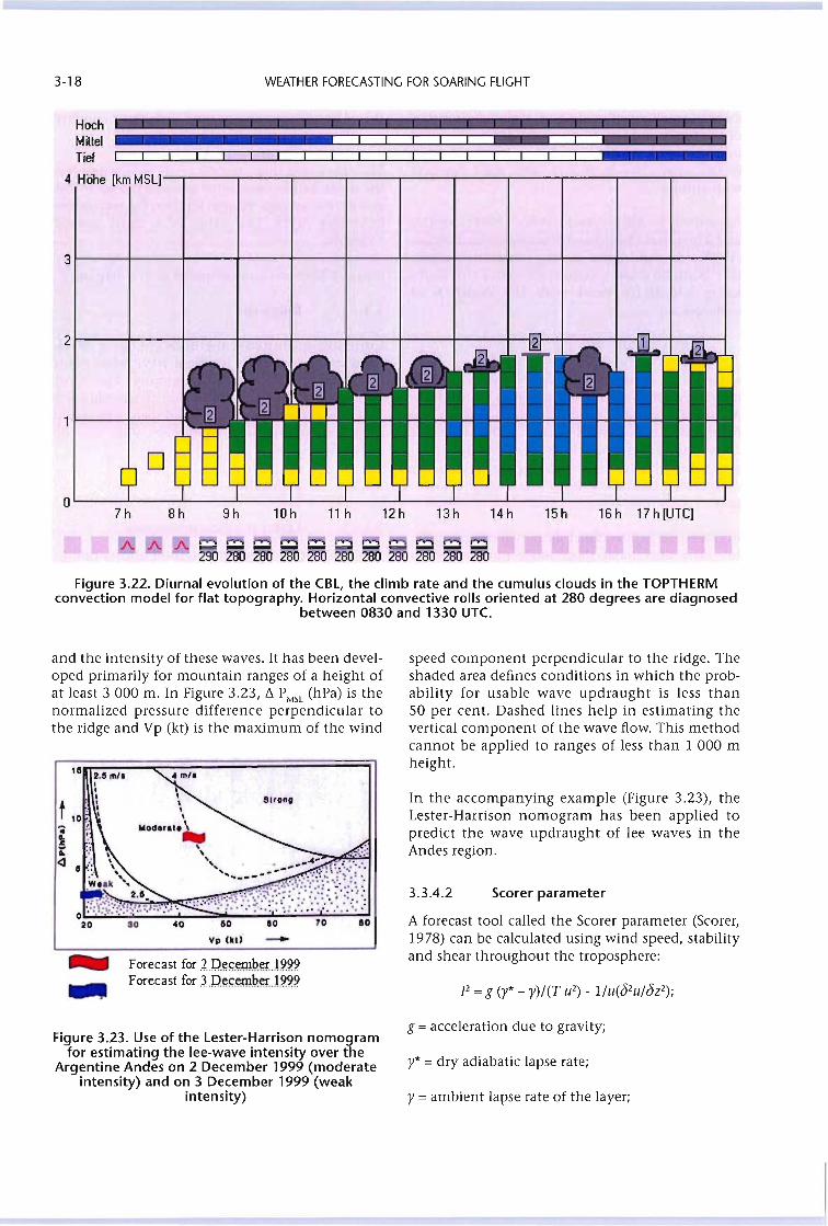
3-18 WEATHER FORECASTING FOR SOARING FLIGHT
HochMillelTiel
4 Hohe [km MSL)-,..------,r-------r---,-----,---,---,----.----.------,-----,
31----I-------ir------ir------i----i----i----t----t----+----+----+------t
2t---+----t----+---i---+---+----+-----t--; I---+----+--i
Ol-__l-__l-_----"l-_----JL....-_----JL....-_----JL....-_----J__---l__---l__---l__--L__-.J
7h 8h 9h 10 h 11 h 12 h 13 h 14 h 15 h 16 h 17 h [UTe)
Figure 3.22. Diurnal evolution of the CBL, the climb rate and the cumulus clouds in the TOPTHERMconvection model for flat topography. Horizontal convective rolls oriented at 280 degrees are diagnosed
between 0830 and 1330 UTC.
and the intensity of these waves. It has been developed primarily for mountain ranges of a height ofat least 3 000 m. In Figure 3.23, D. PMSL (hPa) is thenormalized pressure difference perpendicular tothe ridge and Vp (kt) is the maximum of the wind
A forecast tool called the Scorer parameter (Scorer,1978) can be calculated using wind speed, stabilityand shear throughout the troposphere:
Scorer parameter3.3.4.2
In the accompanying example (Figure 3.23), theLester-Harrison nomogram has been applied topredict the wave updraught of lee waves in theAndes region.
speed component perpendicular to the ridge. Theshaded area defines conditions in which the probability for usable wave updraught is less than50 per cent. Dashed lines help in estimating thevertical component of the wave flow. This methodcannot be applied to ranges of less than 1 000 mheight.
10
Strong
40 50 eo 70
vp (kl)
Forecast for 200P..~!;.~Q~ ..1.9.9.9.Forecast for J.P..~!;.~Q~..1.9.9.9.--
Figure 3.23. Use of the Lester-Harrison nomogramfor estimating the lee-wave intensity over the
Argentine Andes on 2 December 1999 (moderateintensity) and on 3 December 1999 (weak
intensity)
g = acceleration due to gravity;
y* =dry adiabatic lapse rate;
y = ambient lapse rate of the layer;
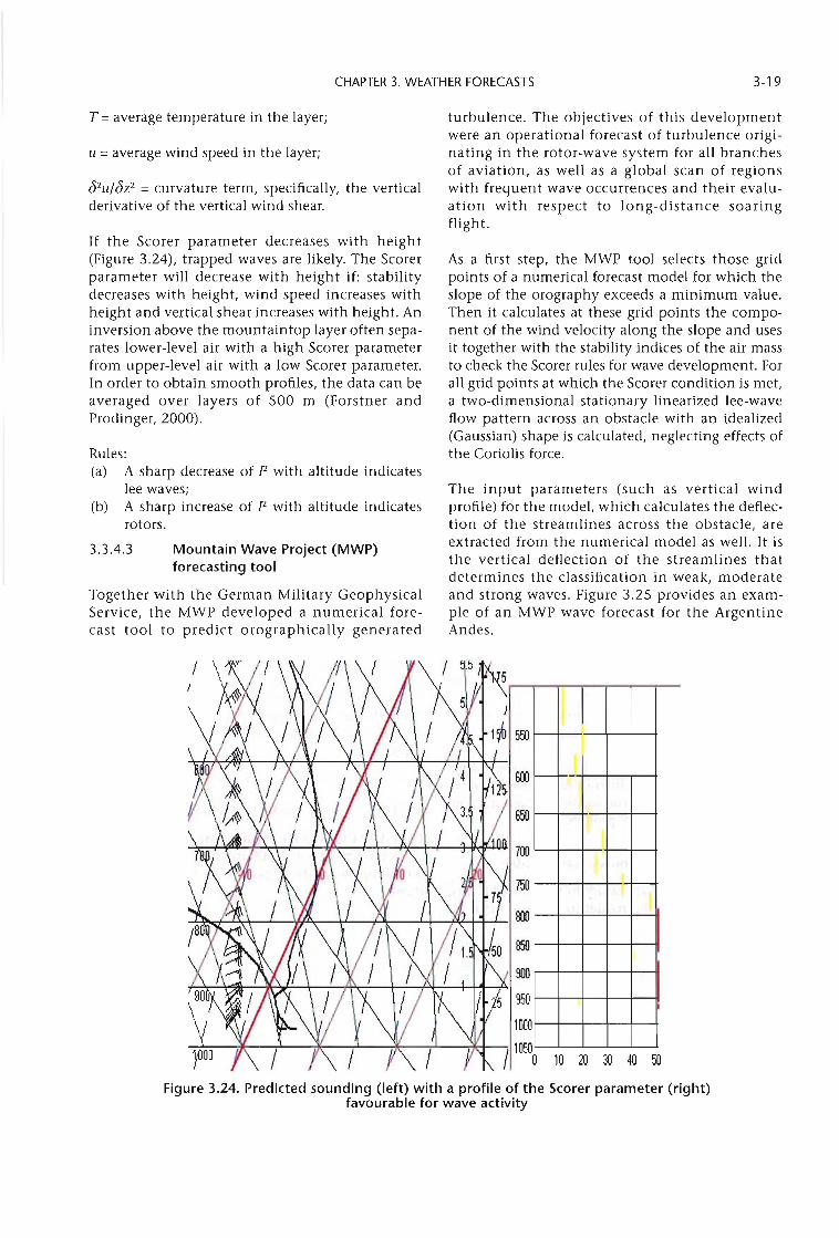
CHAPTER 3. WEATHER FORECASTS 3-19
3.3.4.3
T = average temperature in the layer;
u = average wind speed in the layer;
62u/6z2 = curvature term, specifically, the verticalderivative of the vertical wind shear.
If the Scorer parameter decreases with height(Figure 3.24), trapped waves are likely. The Scorerparameter will decrease with height if: stabilitydecreases with height, wind speed increases withheight and vertical shear increases with height. Aninversion above the mountaintop layer often separates lower-level air with a high Scorer parameterfrom upper-level air with a low Scorer parameter.In order to obtain smooth profiles, the data can beaveraged over layers of 500 m (Forstner andProdinger, 2000).
Rules:(a) A sharp decrease of F with altitude indicates
lee waves;(b) A sharp increase of F with altitude indicates
rotors.
Mountain Wave Project (MWP)forecasting tool
Together with the German Military GeophysicalService, the MWP developed a numerical forecast tool to predict orographically generated
/I
turbulence. The objectives of this developmentwere an operational forecast of turbulence originating in the rotor-wave system for all branchesof aviation, as well as a global scan of regionswith frequent wave occurrences and their evaluation with respect to long-distance soaringflight.
As a first step, the MWP tool selects those gridpoints of a numerical forecast model for which theslope of the orography exceeds a minimum value.Then it calculates at these grid points the component of the wind velocity along the slope and usesit together with the stability indices of the air massto check the Scorer rules for wave development. Forall grid points at which the Scorer condition is met,a two-dimensional stationary linearized lee-waveflow pattern across an obstacle with an idealized(Gaussian) shape is calculated, neglecting effects ofthe Coriolis force.
The input parameters (such as vertical windprofile) for the model, which calculates the deflection of the streamlines across the obstacle, areextracted from the numerical model as well. It isthe vertical deflection of the streamlines thatdetermines the classification in weak, moderateand strong waves. Figure 3.25 provides an example of an MWP wave forecast for the ArgentineAndes.
10 20 30 40 50
Figure 3.24. Predicted sounding (left) with a profile of the Scorer parameter (right)favourable for wave activity
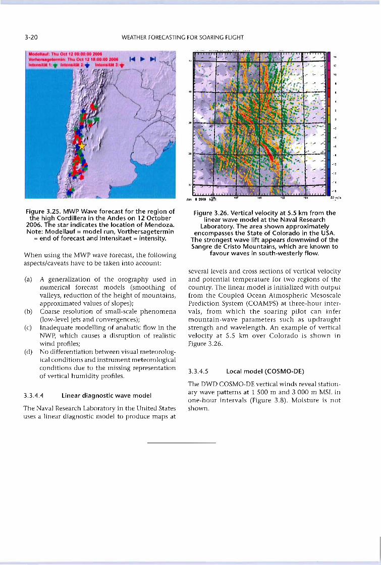
3-20 WEATHER FORECASTING FOR SOARING FLIGHT
",.
.,-.-..a
-..-1l
-14
-la
Ion J~ny's
The Naval Research Laboratory in the United Statesuses a linear diagnostic model to produce maps at
When using the MWP wave forecast, the followingaspects/caveats have to be taken into account:
Figure 3.25. MWP Wave forecast for the region ofthe high Cordillera in the Andes on 12 October
2006. The star indicates the location of Mendoza.Note: Modellauf = model run, Vorthersagetermin
=end of forecast and intensitaet =intensity.
(a) A generalization of the orography used innumerical forecast models (smoothing ofvalleys, reduction of the height of mountains,approximated values of slopes);
(b) Coarse resolution of small-scale phenomena(low-level jets and convergences);
(c) Inadequate modelling of anabatic flow in theNWP, which causes a disruption of realisticwind profiles;
(d) No differentiation between visual meteorological conditions and instrument meteorologicalconditions due to the missing representationof vertical humidity profiles.
Local model (COS MO-DE)3.3.4.5
Figure 3.26. Vertical velocity at 5.5 km from thelinear wave model at the Naval Research
Laboratory. The area shown approximatelyencompasses the State of Colorado in the USA.
The strongest wave lift appears downwind of theSangre de Cristo Mountains, which are known to
favour waves in south-westerly flow.
several levels and cross sections of vertical velocityand potential temperature for two regions of thecountry. The linear model is initialized with outputfrom the Coupled Ocean Atmospheric MesoscalePrediction System (COAMPS) at three-hour intervals, from which the soaring pilot can infermountain-wave parameters such as updraughtstrength and wavelength. An example of verticalvelocity at 5.5 km over Colorado is shown inFigure 3.26.
The DWD COSMO-DE vertical winds reveal stationary wave patterns at 1 500 m and 3 000 m MSL inone-hour intervals (Figure 3.8). Moisture is notshown.
linear diagnostic wave model3.3.4.4
CHAPTER 4
METEOROLOGICAL SUPPORT FOR SOARING FLIGHT
The rapid development of the means of communication over the past decade has resulted in manydifferent information sources with a vast array ofmeteorological data and products useful for soaringpurposes. The individual retrieval and analysis ofthis weather information from the Internet or viaspecial briefing facilities is called"self-briefing" or"home-briefing".
A possible timetable of preparations for a competition may look like this:
t-180 min Analysis of the latest surface andupper-air charts and of the current weathersituation (radar, satellite, webcams, mesonetstations)
4.1 SELF-BRIEFING 4.2.1 Meteorological support forcompetitions
The nearly unlimited sources of weather information often lead to more confusion than help formeteorologists and pilots in the decision-makingprocess. With a view to addressing this problem, apossible scheme for glider pilots' self-briefing isprovided below (Table 4.1). This recommendedscheme is the result of discussions with glider pilotsduring meteorological seminars and it is employedin pcmet, the DWD online self-briefing systemthat is widely used in Europe. It should be stressedthat this scheme is one possible gUideline for theself-briefing of glider pilots for soaring activities,especially in central Europe. Depending on localconditions (weather, available data and products),another scheme may be better for other areas.
t-160 min Checking the models: limited areamodels (two-dimensional charts, soundingforecasts), special local models
t-140 min Forecast of the surface wind for theexpected runway to use (gridding ofthe gliders),first guess of the tasks with task-setter(s): flyable area and duration of flyable conditions
t-120 min Comparison of models with the actualconditions and identification of corrections
t-lOO min Coordinating the meteorologicalconditions with the provisional tasks set bythe task-setter, preparing alternatives, if necessary
4.2 PERSONAL BRIEFINGt-75 min Monitoring the conditions for the
prepared task(s) and feedback loop with thetask-setter
4.2.2 Preparation of soaring forecasts
t-take off Monitoring: unexpected changes,hazards - communication with the organizer
t-60 min Preparation of the weather briefingusing, for example, the PowerPoint program
Successful forecasting for soaring is a major challenge for meteorologists and depends on detailedanalysis concentrated upon a relatively smallarea. The necessary work consists mainly ofthree parts: the synoptic analysis of the actualweather at the surface and the upper air, theinterpretation of the numerical model outputsand their comparison with the actual weathersituation.
Weather briefing for pilotst-O min
In this context "personal briefing" is defined asproviding, in person, tailored meteorological information in a short and concise way to glider pilots.Despite today's highly sophisticated model forecasts, personal briefings are still a benefit forplanning flight tasks. There are different requirements, of course, depending on the event (such ascompetitions, camps or safaris). For competitionsin particular it is valuable to have a meteorologiston site, preferably someone who is familiar withgliding weather of the local area. The competitionmeteorologist plays a key role in:(a) Supporting operations with forecasts of
surface wind for the expected runway to use;(b) Planning the tasks and supporting the task
setter with detailed information;(c) Preparing and presenting the weather briefing
for the competitors;(d) Monitoring the meteorological conditions,
especially hazardous weather.
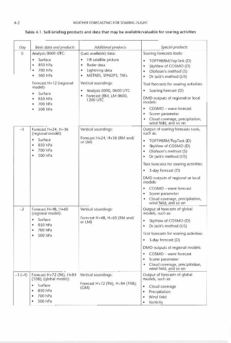
4-2 WEATHER FORECASTING FOR SOARING FLIGHT
Table 4.1. Self-briefing products and data that may be available/valuable for soaring activities
Day Basic data and products Additional products Special products
0 Analysis 0000 UTC: (Last available) data: Soaring forecasts tools:
• Surface • HR satellite picture • TOPTHERM/TopTask (D)• 850 hPa • Radar data • SkyView of COSMO (D)• 700 hPa • Lightning data • Olofsson's method (S)• 500 hPa • METARS, SYNOPS, TAFs • Dr Jack's method (US)
Forecast H+12 (regional Vertical soundings: Text forecasts for soaring activities:model):
• Analysis 0000, 0600 UTC • Soaring forecast (D)• Surface • Forecast (RM, LM 0600,
DMD outputs of regional or local• 850 hPa 1200 UTC• 700 hPa models:
• 500 hPa • COSMO - wave forecast
• Scorer parameter
• Cloud coverage, precipitation,wind field, and so on.
-1 Forecast H+24, H+36 Vertical soundings: Output of soaring forecasts tools,(regional model): such as:
• Surface Forecast H+24, H+36 (RM and/• TOPTHERM/TopTask (D)or LM)
• 850 hPa • SkyView of COSMO (D)• 700 hPa • Olofsson's method (S)• 500 hPa • Dr Jack's method (US)
Text forecasts for soaring activities:
• 3-day forecast (D)
DMD outputs of regional or localmodels:
• COSMO - wave forecast
• Scorer parameter
• Cloud coverage, precipitation,wind field, and so on
-2 Forecast H+48, H+60 Vertical soundings: Output of forecasts of global(regional model): models, such as:
• Surface Forecast H+48, H+60 (RM and/SkyView of COSMO (D)or LM) •
• 850 hPa • Dr Jack's method (US)• 700 hPa
• 500 hPa Text forecasts for soaring activities:
• 3-day forecast (D)
DMO outputs of regional models:
• COSMO - wave forecast
• Scorer parameter
• Cloud coverage, precipitation,wind field, and so on
-3 (-4) Forecast H+72 (96), H+84 Vertical soundings: Output of forecasts of global(108); (global model): models, such as:
• Surface Forecast H+72 (96), H+84 (108);Cloud coverage(GM) •
• 850 hPa • Precipitation• 700 hPa • Wind field• 500 hPa • Vorticity
CHAPTER 4. METEOROLOGICAL SUPPORT FOR SOARING FLIGHT 4-3
A detailed analysis of the current weather situationis important to get an overall view of the weather. Ifthere is no way to analyse surface and upper-aircharts, charts issued by major meteorological services may help and save time. The folloWing areimportant weather features to look for in the various sources of data:(a) Latest surface chart:
(i) Pressure field, isallobaric fields, pressurecentres and their movement;
(ii) Frontal zones with or without precipitation,convergence lines and their movement;
(iii) Observed cloud types in different levels(for example, Ac cas as an indication ofan upper air destabilization, Ac len formountain waves);
(iv) Rainfall amount of the previous day inthe surrounding area;
(v) Dewpoint analysis;(vi) Hazards (thunderstorms, squall lines,
hail) in the upstream area;(b) Upper-air charts (0000 and 1200 UTC):
(i) Jet stream positions at 300 hPa (left orright exit of jet streaks) and movement;
(ii) Geopotential field, trough and ridge positions and their movement at 500 hPa;
(iii) Air mass analysis: temperature gradientsand advection at 850 and 700 hPa;
(iv) Wind and humidity fields at 850 and 700hPa;
(c) Satellite, radar pictures, webcams, windprofiler and mesonet stations:(i) Development and formations of clouds,
frontal structures and associated movement;
(ii) Radar echoes, weakening or intensifyingof rain bands or convective systems;
(iii) Current wind and temperature distribution;
(d) Soundings:(i) Nearest station;(ii) Upstream soundings;(iii) Making a local sounding by plane or
model plane could be helpful;(e) Special observations:
(i) METAR (current weather);(ii) AIRMET, GAMET, SIGMET (current and
forecast hazardous weather);(iii) PIREPS (Pilot reports).(iv) Numerical model output
4.2.3 Meteorological support for thetask-setter
If any of the features mentioned above, determinedfrom prevailing conditions, are different from themodel forecast, adjustments are necessary.
Numerical forecasts need to be compared with theanalyses, if possible by employing the NWP LMand special tools (such as TOPTHERM) that useboundary conditions of the LM. If the model forecasts fit well to the latest analysis (for example, the0000 UTC model run valid at 0600 UTC fits theactual 0600 UTC analysis), then you can trust themodel.
Comparison
(b) Influence of jet streams;(c) Movement of frontal systems;(d) Advection of temperature and humidity,
clouds at different levels;(e) Wind fields at different heights;(t) Change in surface pressure;(g) Stability of the atmosphere (forecast sound
ings);(h) Identification of mesoscale structures (meso
low, low-level jet).
In the unlikely event of a communication failure,which would mean that no forecast soundings frommodels are available, the "classic" analysis and forecast method using actual soundings (perhaps froma tug aircraft) is required to assess the impact ofhorizontal advection of temperature and/or humidity. There is software available that easily calculatesand displays the change of the vertical profile intime (see section 3.3.1.1).
4.2.2.2
Special attention should be paid to:(a) More or fewer layer clouds than forecasted
that could weaken or strengthen the convection;
(b) Earlier or later development of convectionand its strength;
(c) Reinforcement or weakening of nearby fronts;(d) Change of wind direction and/or speed at
different levels;(e) Higher or lower temperature at the surface
(which affects the start time of convection);(t) Existence of inversions not forecast (local
effects, in mountainous areas especially).
Analysis4.2.2.1
The model output should be checked critically. Theimportant features to look for are:(a) Development of troughs and ridges (large
scale vertical motion and vorticity advection);
Setting good tasks in terms of direction and distanceis a challenging job. Depending upon the weathersituation, the orographic conditions and theperformance of the gliders, the task-setter has to
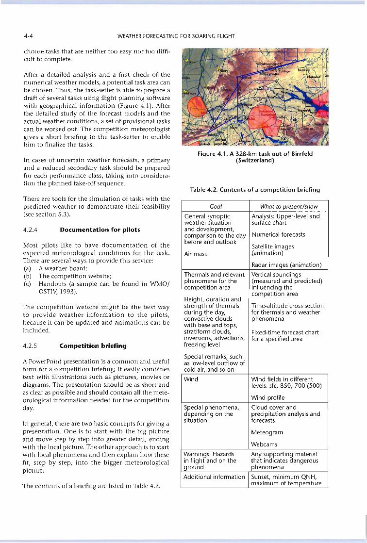
4-4 WEATHER FORECASTING FOR SOARING FLIGHT
choose tasks that are neither too easy nor too difficult to complete.
After a detailed analysis and a first check of thenumerical weather models, a potential task area canbe chosen. Thus, the task-setter is able to prepare adraft of several tasks using flight planning softwarewith geographical information (Figure 4.1). Afterthe detailed study of the forecast models and theactual weather conditions, a set of provisional taskscan be worked out. The competition meteorologistgives a short briefing to the task-setter to enablehim to finalize the tasks.
In cases of uncertain weather forecasts, a primaryand a reduced secondary task should be preparedfor each performance class, taking into consideration the planned take-off sequence.
There are tools for the simulation of tasks with thepredicted weather to demonstrate their feasibility(see section 5.3).
4.2.4 Documentation for pilots
Most pilots like to have documentation of theexpected meteorological conditions for the task.There are several ways to provide this service:(a) A weather board;(b) The competition website;(c) Handouts (a sample can be found in WMO/
OSTIV, 1993).
The competition website might be the best wayto provide weather information to the pilots,because it can be updated and animations can beincluded.
4.2.5 Competition briefing
A PowerPoint presentation is a common and usefulform for a competition briefing; it easily combinestext with illustrations such as pictures, movies ordiagrams. The presentation should be as short andas clear as possible and should contain all the meteorological information needed for the competitionday.
In general, there are two basic concepts for giving apresentation. One is to start with the big pictureand move step by step into greater detail, endingwith the local picture. The other approach is to startwith local phenomena and then explain how thesefit, step by step, into the bigger meteorologicalpicture.
The contents of a briefing are listed in Table 4.2.
Figure 4.1. A 328-km task out of Birrfeld(Switzerland)
Table 4.2. Contents of a competition briefing
Goal What to present/show
General synoptic Analysis: Upper-level andweather situation surface chartand development,
Numerical forecastscomparison to the daybefore and outlook
Satellite imagesAir mass (animation)
Radar images (animation)
Thermals and relevant Vertical soundingsphenomena for the (measured and predicted)competition area influencing the
Height, duration andcompetition area
strength of thermals Time-altitude cross sectionduring the day, for thermals and weatherconvective clouds phenomenawith base and tops,stratiform clouds, Fixed-time forecast chartinversions, advections, for a specified areafreezing level
Special remarks, suchas low-level outflow ofcold air, and so on
Wind Wind fields in differentlevels: sk, 850, 700 (500)
Wind profile
Special phenomena, Cloud cover anddepending on the precipitation analysis andsituation forecasts
Meteogram
Webcams
Warnings: Hazards Any supporting materialin flight and on the that indicates dangerousground phenomena
Additional information Sunset, minimum QNH,maximum of temperature
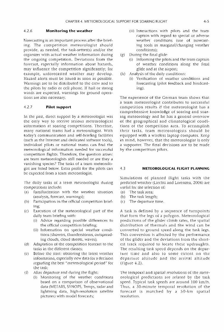
CHAPTER 4. METEOROLOGICAL SUPPORT FOR SOARING FLIGHT 4-5
The temporal and spatial resolutions of the meteorological predictions are related by the taskspeed. Typical task speeds are around 100 km/h.Thus, a 30-minute temporal resolution of theforecast is matched by a 50-km spatialresolution.
Simulations of planned flight tasks with thepredicted weather (Liechti and Lorenzen, 2004) areuseful for the selection of:(a) The task area;(b) The task length;(c) The departure time.
The experience of the German team shows thata team meteorologist contributes to successfulcompetition results if the meteorologist has acomprehensive knowledge of soaring and soaring meteorology and he has a general overviewof the geographical and climatological conditions of the competition area. To accomplishtheir tasks, team meteorologists should beequipped with a wireless laptop computer. Keepin mind, however, that the meteorologist is onlya supporter. The final decisions are to be madeby the competition pilots.
A task is defined by a sequence of turnpointsthat form the legs of a polygon. Meteorologicalpredictions of the glider climb rates, the spatialdistribution of thermals and the wind can beconverted to ground speed along the task legs.This conversion is affected by the performanceof the glider and the deviations from the shortest track required to locate these updraughts.The resulting task speed depends on the departure time and also to some extent on thedeparture altitude and the arrival altitude(Figure 4.2).
METEOROLOGICAL FLIGHT PLANNING4.3
(ii) Interactions with pilots and the teamcaptain with regard to special or adverseweather conditions (use of nowcasting tools in marginal/changing weatherconditions);
(g) During the final glide:(i) Informing the pilots and the team captain
of weather conditions along the finalglide and at the airport;
(h) Analysis of the daily conditions:(i) Verification of weather conditions and
forecasting (pilot feedback and hindcasting).
4.2.7 Pilot support
Nowcasting is an important process after the briefing. The competition meteorologist shouldprovide, as needed, the task-setter(s) and/or theorganizer with actual weather information duringthe ongoing competition. Deviations from theforecast, especially information about hazards,may influence the competition significantly; forexample, unforecasted weather may develop.Hazard alerts must be issued as soon as possible.Warnings are to be distributed to the crew and tothe pilots by radio or cell phone. If hail or strongwinds are expected, warnings for ground operations are also necessary.
In the past, direct support by a meteorologist wasthe only way to receive serious meteorologicalinformation at soaring competitions. Therefore,many national teams had a meteorologist. Withtoday's communication and self-briefing facilities(such as the Internet and dedicated software tools),individual pilots or national teams can find themeteorological information needed for successfulcompetition flights. Therefore, the question arises:are team meteorologists still needed or are they avanishing species? The tasks of a team meteorologist are listed below. Extra profit for the pilots canbe expected from a team meteorologist.
The daily tasks of a team meteorologist duringcompetitions include:(a) Familiarization with the weather situation
(analysis, forecast, warnings);(b) Participation in the official competition brief
ing;(c) Execution of the meteorological part of the
daily team briefing with:(i) Advice regarding possible differences to
the official competition briefing;(ii) Information on special weather condi
tions (showers, thunderstorms, outspreading clouds, cloud streets, waves);
(d) Adaptation of the competition forecast to thetasks in the different classes;
(e) Before the start: obtaining the latest weatherinformation, especially new data for a decisionregarding the best "meteorological period" forthe task;
(t) After departure and during the flight:(i) Monitoring of the weather conditions
based on a comparison of observationaldata (METARS, SYNOPS, Temps, radar andlightning data, high-resolution satellitepictures) with model forecasts;
4.2.6 Monitoring the weather
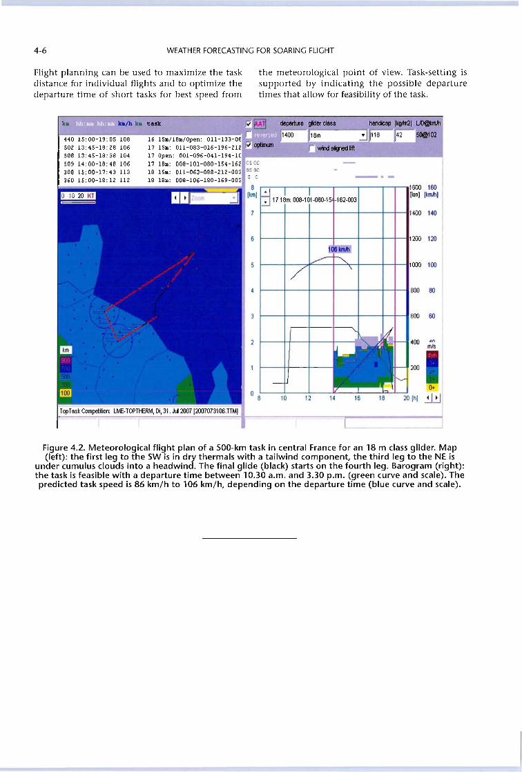
4-6 WEATHER FORECASTING FOR SOARING FLIGHT
Flight planning can be used to maximize the taskdistance for individual flights and to optimize thedeparture time of short tasks for best speed from
the meteorological point of view. Task-setting issupported by indicating the possible departuretimes that allow for feasibility of the task.
.nmls
0+
20 (h) ~1816141210
r-;--,---.---,---r--,-.----.1600 160(km] [km.tl]
1--+--+--+---+---+-+--11400 140
1--+--+--+---+---+-+--11200 120
1--+--+--+---+---+-+--1800 80 I
1--+--7I'C---+-~-+---+-+--IlO00 100
f---+-----f--+----+--t-+-I600 60
16 15./18./0pen: 011-133-0E17 15.: 011-083-016-196-21217 Open: 001-096-041-194-1(1r- ~ ~ _I
17 18.: 008-101-080-154-16218 15.: 011-063-088-212-00<18 18.: 008-106-180-169-00<
440 15:00-19:05 108502 13:45-18:28 106508 13:45-18:38 104509 14:00-18:48 106308 15:00-17:43 113360 15:00-18:12 112
TopTask Compel~ion: LME.TOPTHERM, Di, 31. Jul2OO7 (2007073106.TTM)___I - -- __un_.
ka
Figure 4.2. Meteorological flight plan of a SOO-km task in central France for an 18 m class glider. Map(left): the first leg to the SW is in dry thermals with a tailwind component, the third leg to the NE is
under cumulus clouds into a headwind. The final glide (black) starts on the fourth leg. Barogram (right):the task is feasible with a departure time between 10.30 a.m. and 3.30 p.m. (green curve and scale). Thepredicted task speed is 86 km/h to 106 km/h, depending on the departure time (blue curve and scale).

CHAPTER 5
FLIGHT DATA
5.1
5.1.1
FLIGHT DOCUMENTATION
Flight recorder
are a result of the solar irradiation and the horizontal airflow interacting with the terrain. The analysisof these positions reveals the meteorological processes at work.
For all badge, competition and record flights, anInternational Gliding Commission (IGC)approved documentation of the flight ismandatory. This is usually accomplished by usinga "secure" GPS-based flight recorder that storesthree-dimensional position data and additionalbarometric pressure in a secure data file called anIGC-file. An on-board navigation (NAV) computerderives real-time ground speed, as well as the windcomponent along the direction of flight, fromthese data. If heading information is available,full-vector wind determination becomes feasible.Some NAV/final-glide computers use temperaturesensors to calculate true airspeed at altitude andpotential temperature.
5.1.2 Flight data analysis
The data from the IGC-file allow for some postflight analysis. Various visualization tools areavailable to plot, for example, an altitude traceversus time or a two-dimensional flight track. A fullthree-dimensional representation of the flight dataalso can be displayed using the popular GoogleEarth software, which accepts the IGC data format.Flight data are also a rich source of information onmeteorological processes.
5.1.3 Flight data sources
The relevant IGC-files can be used to compile statistics of achieved distances and speeds of a number offlights in a given area or over a given period. Theseare available from the international Online Contest(OLC) for most active gliding regions around theglobe, or, for localized events, from the mainnational and international competition sites. Thelatter, in particular, are suitable for verification ofthe forecasts given.
5.2 POSITION OF UPDRAUGHTS
Updraughts can be identified in recorded flight dataand atmospheric lift patterns can be recognized.The positions of thermal lift, ridge lift and wave lift
5.2.1 Thermal lift
The combination of high-resolution topographicaldata and the diurnal and seasonal variation of solarirradiation has been visualized by Heise (1999) andrefined by Sigrist (2006) as TherMaps. These mapsare calculated for fixed times and dates. Clear sky isassumed and seasonal variations in the surfaceparameters controlling the albedo (snow line) andthe evapotranspiration (vegetation) are included.Furthermore, the significant phase shift of severalhours between the irradiation and the resultingupdraughts is modelled. In mountainous areas suchas the Alps, the Pyrenees and the Apennines, aTherMap analysis of flight data reveals that ascentsin thermal lift are located above computed hotspots in numerous cases.
The visualization of flight tracks on TherMapsconfirms that slopes significantly affect thespatial distribution of lift used for thermal soaring(Figure 5.1). It suggests that high-resolution fore-
Figure 5.1. Recorded flight track on a TherMaprendered in 3D. The climbing segments (red
portion of the flight track) are confirmed by thecomputed hot spots (brown-to-red surfaces).
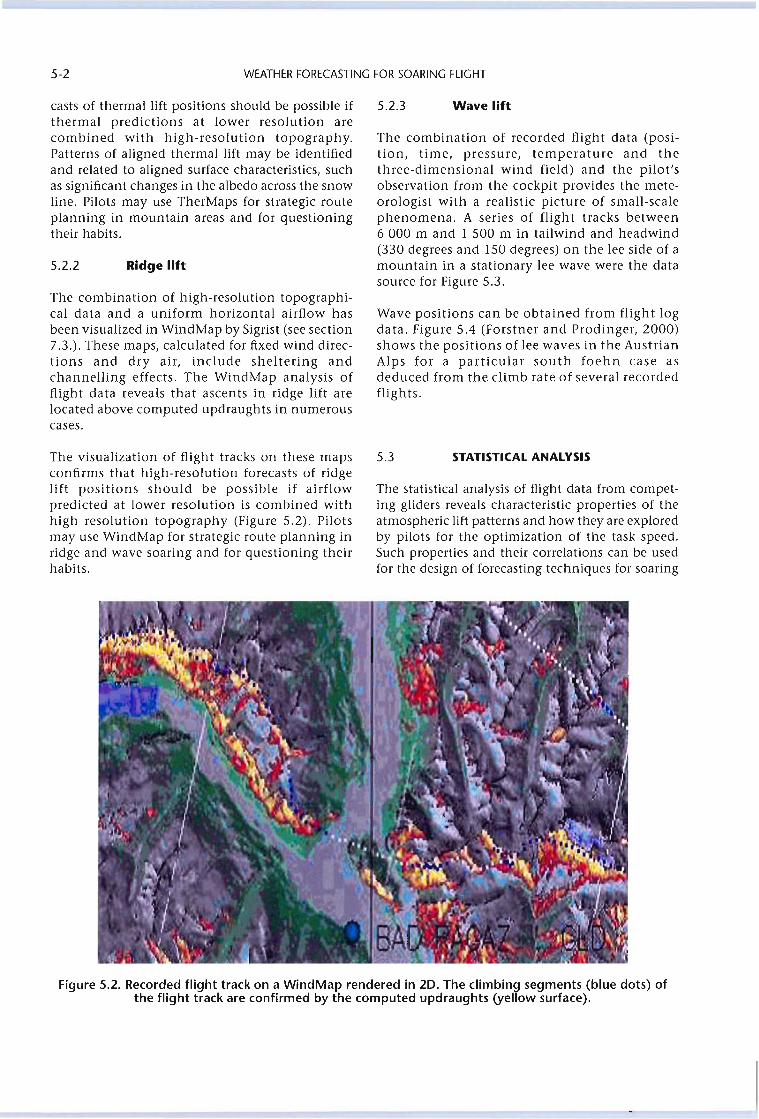
5-2 WEATHER FORECASTING FOR SOARING FLIGHT
casts of thermal lift positions should be possible ifthermal predictions at lower resolution arecombined with high-resolution topography.Patterns of aligned thermal lift may be identifiedand related to aligned surface characteristics, suchas significant changes in the albedo across the snowline. Pilots may use TherMaps for strategic routeplanning in mountain areas and for questioningtheir habits.
5.2.2 Ridge lift
The combination of high-resolution topographical data and a uniform horizontal airflow hasbeen visualized in WindMap by Sigrist (see section7.3.). These maps, calculated for fixed wind directions and dry air, include sheltering andchannelling effects. The WindMap analysis offlight data reveals that ascents in ridge lift arelocated above computed updraughts in numerouscases.
The visualization of flight tracks on these mapsconfirms that high-resolution forecasts of ridgelift positions should be possible if airflowpredicted at lower resolution is combined withhigh resolution topography (Figure 5.2). Pilotsmay use WindMap for strategic route planning inridge and wave soaring and for questioning theirhabits.
5.2.3 Wave lift
The combination of recorded flight data (position, time, pressure, temperature and thethree-dimensional wind field) and the pilot'sobservation from the cockpit proVides the meteorologist with a realistic picture of small-scalephenomena. A series of flight tracks between6 000 m and 1 500 m in tailwind and headwind(330 degrees and 150 degrees) on the lee side of amountain in a stationary lee wave were the datasource for Figure 5.3.
Wave positions can be obtained from flight logdata. Figure 5.4 (Forstner and Prodinger, 2000)shows the positions of lee waves in the AustrianAlps for a particular south foehn case asdeduced from the climb rate of several recordedflights.
5.3 STATISTICAL ANALYSIS
The statistical analysis of flight data from competing gliders reveals characteristic properties of theatmospheric lift patterns and how they are exploredby pilots for the optimization of the task speed.Such properties and their correlations can be usedfor the design of forecasting techniques for soaring
Figure 5.2. Recorded flight track on a WindMap rendered in 2D. The climbing segments (blue dots) ofthe flight track are confirmed by the computed updraughts (yellow surface).
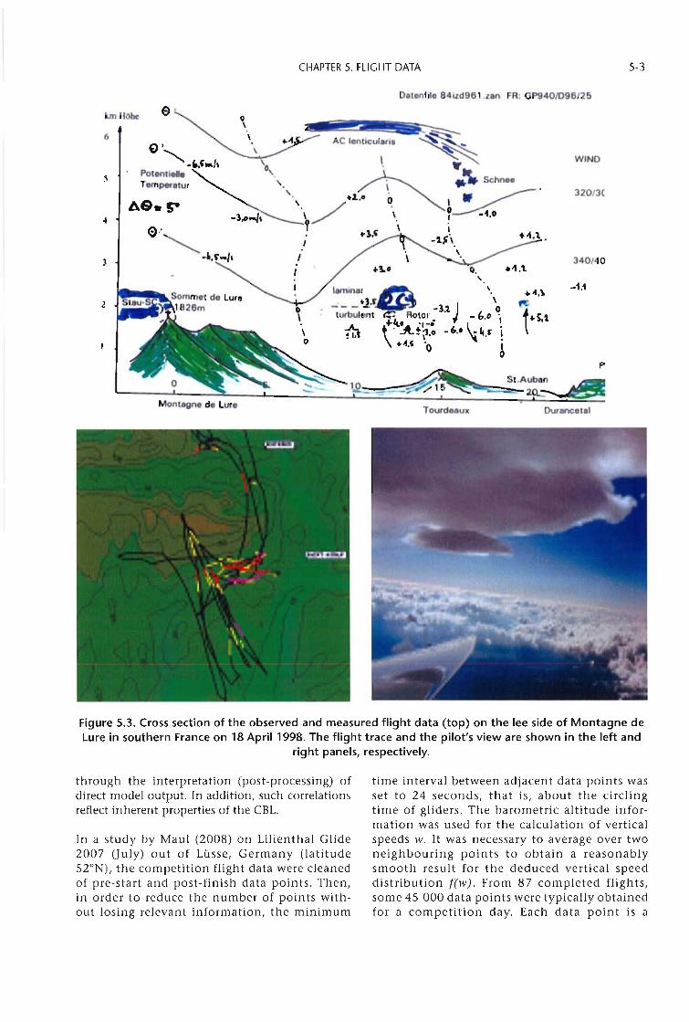
CHAPTER 5. FLIGHT DATA
Ollonll.o 84ild961.lan FR: GP9401096/25
5-3
kmHObe ,6
"5
A6.S-4
e"~
) ....~\.."2
10
WIND
320/3C
340/40
Figure 5.3. Cross section of the observed and measured flight data (top) on the lee side of Montagne delure in southern France on 18 April 1998. The flight trace and the pilot's view are shown in the left and
right panels, respectively.
through the interpretation (post-processing) ofdirect model output. In addition, such correlationsreflect inherent properties of the CBL.
In a study by Maul (2008) on Lilienthal Glide2007 (July) out of Ltisse, Germany (latitudeS2°N), the competition flight data were cleanedof pre-start and post-finish data points. Then,in order to reduce the number of points without losing relevant information, the minimum
time interval between adjacent data points wasset to 24 seconds, that is, about the circlingtime of gliders. The barometric altitude information was used for the calculation of verticalspeeds w. It was necessary to average over twoneighbouring points to obtain a reasonablysmooth result for the deduced vertical speeddistribution few}. From 87 completed flights,some 4S 000 data points were typically obtainedfor a competition day. Each data point is a
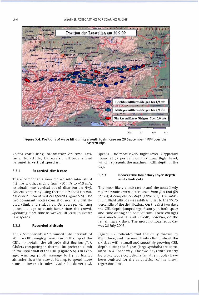
5-4 WEATHER FORECASTING FOR SOARING FLIGHT
Olcrn 50 100 150
Figure 5.4. Positions of wave lift during a south foehn case on 20 September 1999 over theeastern Alps
vector containing information on time, latitude, longitude, barometric altitude z andbarometric vertical speed w.
5.3.1 Recorded climb rate
The w components were binned into intervals of0.2 m/s width, ranging from -10 m/s to +10 m/s,to obtain the vertical speed distribution few).Gliders competing using thermal lift show a bimodal distribution of vertical speeds (Figure 5.5). Thetwo dominant modes consist of normally distributed climb and sink rates. On average, winningpilots manage to climb faster than the crowd.Spending more time in weaker lift leads to slowertask speeds.
5.3.2 Recorded altitude
The z components were binned into intervals ofSO m width, ranging from 0 m to the top of theCBL, to obtain the altitude distribution fez).Gliders competing in thermal lift prefer to climbin the upper half of the CBL (Figure 5.6). On average, winning pilots manage to fly at higheraltitudes than the crowd. Having to spend moretime at lower altitudes results in slower task
speeds. The most likely flight level is typicallyfound at 67 per cent of maximum flight level,which represents the maximum eBL depth of theday.
5.3.3 Convective boundary layer depthand climb rate
The most likely climb rate wand the most likelyflight altitude z were determined from few) and fez)for eight competition days (Table 5.1). The maximum flight altitude was arbitrarily set to the 99.75percentile of the distribution. On the first two daysthe CBL depth jumped significantly in both spaceand time during the competition. These changeswere much smaller and smooth, however, on theremaining six days. The most homogeneous daywas 26 July 2007.
Figure 5.7 indicates that the daily maximumflight level and the most likely climb rate of thesix days with a small and smoothly growing CBLdepth during the flights (large symbols) are correlated in a linear way. The two days with clearlyheterogeneous conditions (small symbols) havebeen omitted for the calculation of the linearregression line.
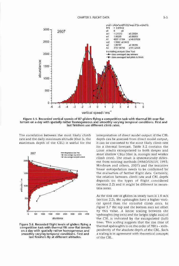
CHAPTER 5. FLIGHT DATA 5-5
6543
y=yO + (A/(w'sqrt(PI/2}))'exp(-2'((x-xc)/w)'2)R'2 = 0.97912yO 0 ±Oxc1 -1.31313 ±0.03024w1 1.80205 ±0.06053A1 4857.17104 ±149.67038xc2 1.5582 ±0.0412w2 1.86767 ±0.08355A2 3757.56744 ±151.32535
thermalling analysis (See You)........ class averaged day winners-T- class averaged last pilots to finish
-2 -1 0 1 2
vertical speed / ms-1
-3-4-5
2607
o+-T""""I-'-6
1000
500
3000
2000
2500
Q)t)
~ 1500"0c::::J.0ro
Figure 5.5. Recorded vertical speeds of 87 gliders flying a competition task with thermal lift over flatterrain on a day with spatially rather homogeneous and smoothly varying temporal conditions. First and
last finishers use different climb rates.
The correlation between the most likely climbrate and the daily maximum altitude (that is, themaximum depth of the CBL) is useful for the
Figure 5.6. Recorded flight levels of gliders flying acompetition task with thermal lift over flat terrainon a day with spatially rather homogeneous andsmoothly varying temporal conditions. First and
last finishers fly at different altitudes.
500 1000 1500 2000 2500 3000 3500 4000
abundance
As the sink rate of gliders in steady turn is 1.0 m/s(section 2.2), the updraughts have a higher vertical speed than the recorded climb rates. InFigure 5.7 the top and the bottom axes are offsetby this value. A linear scaling between theupdraughts (top axis) and the height (right axis) ofthe CBL is indicated by the extrapolated (full)lines. This scaling suggests that the rise time ofthermal updraughts is on the order of 700 s - independently of the absolute depth of the CBL. Sucha scaling is in agreement with theoretical conceptsof the CBL.
interpretation of direct model output: if the CBLdepth can be assessed from direct model output,it can be converted to the most likely climb ratefor a thermal forecast. Table 5.2 contains theLtisse results extrapolated to both deeper andmore shallow CBLs (that is, stronger and weakerclimb rates). The result is systematically different from existing methods (WMO/OSTIV, 1993;Hindman and others, 2007) and the tentativelinear extrapolation needs to be confirmed bythe evaluation of further flight data. Certainly,the relation between climb rate and CBL depthdepends on the types of flight considered(section 2.2) and it might be different in mountain areas.
thermalling analysis (See You)-...- class averaged day winners-T- class averaged lasl pilots 10 finish
2607
EQ)2 100+J(ij
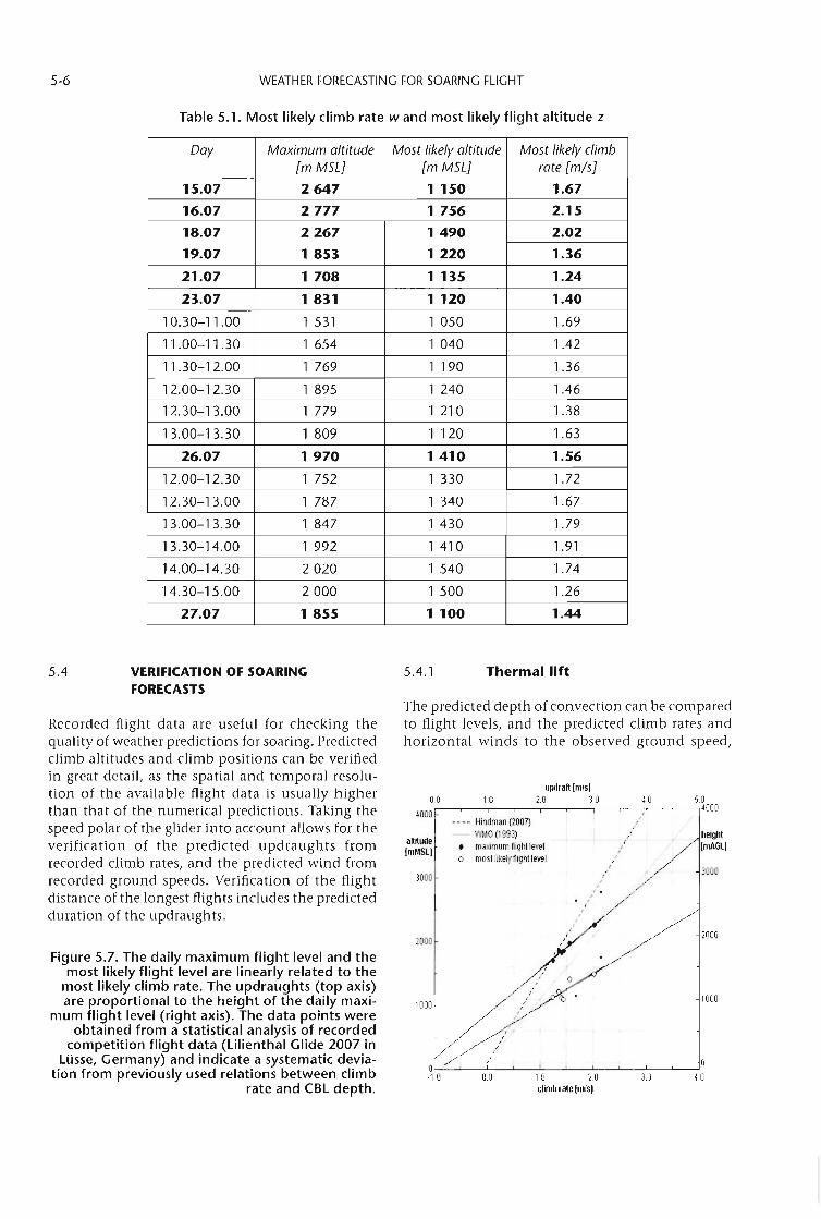
5-6 WEATHER FORECASTING FOR SOARING FLIGHT
Table 5.1. Most likely climb rate wand most likely flight altitude z
Day Maximum altitude Most likely altitude Most likely climb[m MSLj [m MSLj rate [m/sj
15.07 2647 1 150 1.67
16.07 2777 1 756 2.15
18.07 2267 1490 2.02
19.07 1 853 1220 1.36
21.07 1 708 1 135 1.24
23.07 1 831 1 120 1.40
10.30-11.00 1 531 1 050 1.69
11.00-11.30 1 654 1 040 1.42
11.30-12.00 1 769 1 190 1.36
12.00-12.30 1 895 1 240 1.46
12.30-13.00 1 779 1 210 1.38
13.00-13.30 1 809 1 120 1.63
26.07 1970 1410 1.56
12.00-12.30 1 752 1 330 1.72
12.30-13.00 1 787 1 340 1.67
13.00-13.30 1 847 1 430 1.79
13.30-14.00 1 992 1 410 1.91
14.00-14.30 2020 1 540 1.74
14.30-15.00 2000 1 500 1.26
27.07 1 855 1 100 1.44
5.4 VERIFICATION OF SOARING
FORECASTS
5.4.1 Thermal lift
2000
3000
height(rnAGLI
1000
2000
Ulllirafllm/sl0.0 1.0 2.0 30 40 50
4000 .----__~_--H-in.-dm-an-(2.-00-7).......-..----r--~-/.,...'-~---,4000
WMO(1993) /• maximum flighllevel "o most likely ftighllevel ,-
f
,,,,'.
f,,,,,f
,
OL--'-_L--'--_L-~----,.L-~_:L-~----'O-10 0.0 1.0 2.0 30 40
climh rate Im/sl
3000
1000
annudeImlolSLI
The predicted depth of convection can be comparedto flight levels, and the predicted climb rates andhorizontal winds to the observed ground speed,
Figure 5.7. The daily maximum flight level and themost likely flight level are linearly related to the
most likely climb rate. The updraughts (top axis)are proportional to the height of the daily maxi
mum flight level (right axis). The data points wereobtained from a statistical analysis of recorded
competition flight data (Lilienthal Glide 2007 inLLisse, Germany) and indicate a systematic devia
tion from previously used relations between climbrate and CBL depth.
Recorded flight data are useful for checking thequality of weather predictions for soaring. Predictedclimb altitudes and climb positions can be verifiedin great detail, as the spatial and temporal resolution of the available flight data is usually higherthan that of the numerical predictions. Taking thespeed polar of the glider into account allows for theverification of the predicted updraughts fromrecorded climb rates, and the predicted wind fromrecorded ground speeds. Verification of the flightdistance of the longest flights includes the predictedduration of the updraughts.
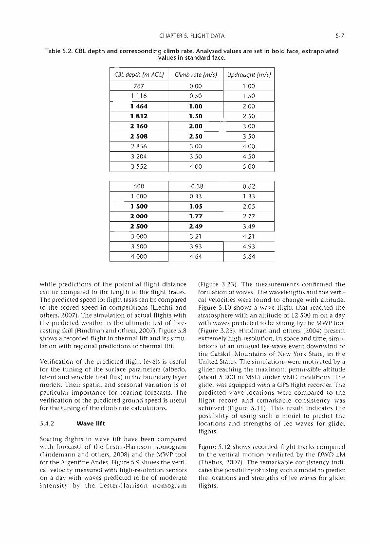
CHAPTER 5. FLIGHT DATA 5-7
Table 5.2. CBL depth and corresponding climb rate. Analysed values are set in bold face, extrapolatedvalues in standard face.
CBL depth [m ACL] Climb rate [m/si Updraught [m/si
767 0.00 1.00
1 116 0.50 1.50
1464 1.00 2.00
1812 1.50 2.50
2160 2.00 3.00
2508 2.50 3.50
2856 3.00 4.00
3204 3.50 4.50
3552 4.00 5.00
500 -0.38 0.62
1 000 0.33 1.33
1 500 1.05 2.05
2000 1.77 2.77
2500 2.49 3.49
3000 3.21 4.21
3500 3.93 4.93
4000 4.64 5.64
while predictions of the potential flight distancecan be compared to the length of the flight traces.The predicted speed for flight tasks can be comparedto the scored speed in competitions (Liechti andothers, 2007). The simulation of actual flights withthe predicted weather is the ultimate test of forecasting skill (Hindman and others, 2007). Figure 5.8shows a recorded flight in thermal lift and its simulation with regional predictions of thermal lift.
Verification of the predicted flight levels is usefulfor the tuning of the surface parameters (albedo,latent and sensible heat flux) in the boundary layermodels. Their spatial and seasonal variation is ofparticular importance for soaring forecasts. Theverification of the predicted ground speed is usefulfor the tuning of the climb rate calculations.
5.4.2 Wave lift
Soaring flights in wave lift have been comparedwith forecasts of the Lester-Harrison nomogram(Lindemann and others, 2008) and the MWP toolfor the Argentine Andes. Figure 5.9 shows the vertical velocity measured with high-resolution sensorson a day with waves predicted to be of moderateintensity by the Lester-Harrison nomogram
(Figure 3.23). The measurements confirmed theformation of waves. The wavelengths and the vertical velocities were found to change with altitude.Figure 5.10 shows a wave flight that reached thestratosphere with an altitude of 12 500 m on a daywith waves predicted to be strong by the MWP tool(Figure 3.25). Hindman and others (2004) presentextremely high-resolution, in space and time, simulations of an unusual lee-wave event downwind ofthe Catskill Mountains of New York State, in theUnited States. The simulations were motivated by aglider reaching the maximum permissible altitude(about 5 200 m MSL) under VMC conditions. Theglider was equipped with a GPS flight recorder. Thepredicted wave locations were compared to theflight record and remarkable consistency wasachieved (Figure 5.11). This result indicates thepossibility of using such a model to predict thelocations and strengths of lee waves for gliderflights.
Figure 5.12 shows recorded flight tracks comparedto the vertical motion predicted by the DWD LM(Thehos, 2007). The remarkable consistency indicates the possibility of using such a model to predictthe locations and strengths of lee waves for gliderflights.
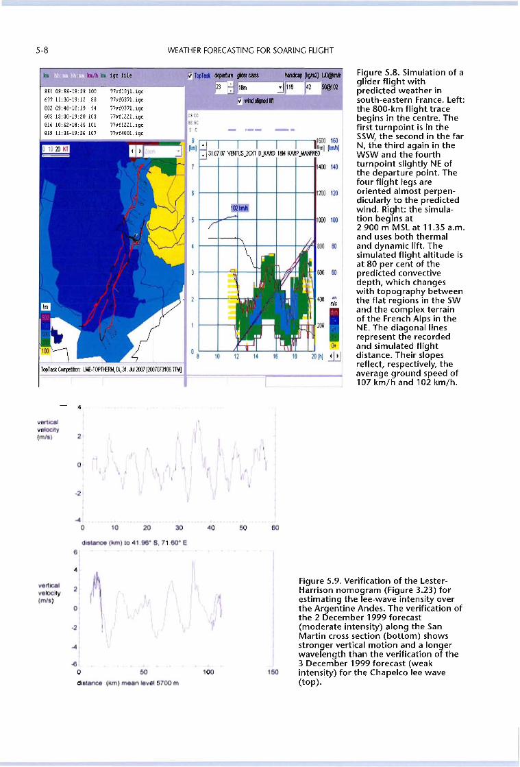
5-8 WEATHER FORECASTING FOR SOARING FLIGHT
Figure 5.8. Simulation of aglider flight withpredicted weather insouth-eastern France. left:the 800-km flight tracebegins in the centre. Thefirst turnpoint is in theSSW, the second in the farN, the third again in theWSW and the fourthturnpoint slightly NE ofthe departure point. Thefour flight legs areoriented almost perpendicularly to the predictedwind. Right: the simulation begins at2 900 m MSl at 11.35 a.m.and uses both thermaland dynamic lift. Thesimulated flight altitude isat 80 per cent of thepredicted convectivedepth, which changeswith topography betweenthe flat regions in the SWand the complex terrainof the French Alps in theNE. The diagonal linesrepresent the recordedand simulated flightdistance. Their slopesreflect, respectively, theaverage ground speed of107 km/h and 102 km/h.
.nrnis
f--f--+--+---f--+---II200 120
f--:J,,...e;"-i---+---f--+---I11))) 100
cs cces8Cse - ._-
77vflOjl. igc
77vf0371. igc
77vf0371. igc
77vflUl. igc
77vflZ21.igc
77vf4001. igc
851 09: 56-18: 28 100
677 11: 30-19: 12 88
80209:48-18:19 94
603 13:30-19:20 103
816 10:52-18:55 101
859 11:35-19:36 107
ka kll/h ka igc filt
TopTes\:~Ut1E.T~TtfRIII, Cl, 31..lJ 2OO7I2007073106.TTh4j
~~~iiiiiiiiiiiiiiiiijiiiiijiiiiiiiiii,1 8 ISXJ 160? [kml: 310707 VOOUSJCXT DJARD HIM KARPJAAI.f~1 [kmti)
f--f--+--+---f--+---II400 140
0+
o8 10 12 14 16 18 20 (hI Mt==~==~~==''=====I
-4
'If IvalOClty 1\(m'l) 2
,\r
'IIi
J ' J •0 I; I ."
·2
~
0 10 20 30 ..0
d (km) 10 .. ,00" S. 11 50"6
..vertl~1 2velocity(mll) I,
0J I,
.~-2
-4.I
.e'0 60 100
dlllllnc (km) m n ......15100m
Figure 5.9. Verification of the lesterHarrison nomogram (Figure 3.23) forestimating the lee-wave intensity overthe Argentine Andes. The verification ofthe 2 December 1999 forecast(moderate intensity) along the SanMartin cross section (bottom) showsstronger vertical motion and a longerwavelength than the verification of the3 December 1999 forecast (weak
HIO intensity) for the Chapelco lee wave(top).
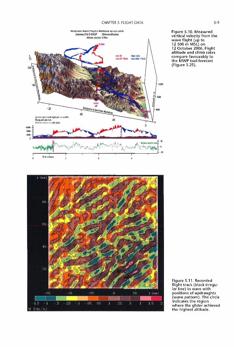
CHAPTER 5. FLIGHT DATA
MUUlIldlll ndV~ "IUJ~l;1 M~IIUU£d 1£ Ul;l £UUD
5temme 510 D·KKOP OhlmannlHackerMitude reached: 12,5km
red: lift blue: sinkmax lift: 15mJs max sink: ·11m1s
12000
8000
4000
Terrain underneath ftightpalh in mAMSLFlying altitude in m 40
12000j VerticalwindinmlS(I::I~ ~ ,~k 0
~
400~~~~ A ~,..,.. ", , -\'."''''>''i' -,~" - \""=- "" --~~~~ - ~/- f'-''''' '-,;, -r-v:;...r,.{ -\" J,...,./1WIt-:;,
E./.;; y .....",..., ' I . 1\,: . (.' '. r'''
~--..2..-='---.---- ----r-------'.--------r-----.---J"" ·10Time in hours
5-9
Figure 5.10. Measuredvertical velocity from thewave flight (up to12500 m MSL) on12 October 2006. Flightaltitude and climb ratescompare favourably tothe MWP tool forecast(Figure 3.25).
Figure 5.11. Recordedflight track (black irregular line) in wave withpositions of updraughts(wave pattern). The circleindicates the regionwhere the glider achievedthe highest altitude.
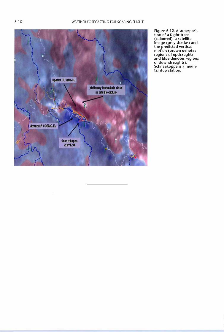
5-10 WEATHER FORECASTING FOR SOARING FLIGHT
Figure 5.12. A superposition of a flight trace(coloured), a satelliteimage (grey shades) andthe predicted verticalmotion (brown denotesregions of updraughtsand blue denotes regionsof downdraughts).Schneekoppe is a mountaintop station.
CHAPTER 6
EPILOGUE
This publication is for all who are concerned withthe meteorological support for gliding. It recordsthe significant progress in weather forecasting forsoaring flight since the 1993 edition of WMOTechnical Note No. 158 Handbook ofMeteorologicalForecasting for Soaring Flight.
In Chapter I, the three main types of lift enablingsoaring flight - convection, ridge and wave lift were described. The physical basis for each wasgiven, providing the meteorologist with theunderstanding to produce meaningful soaringforecasts. Pilot stories describing flights in thethree types of lift illustrated the intimate connection, in the cockpit, between theory andpractice.
The technical description of gliding and soaringflight in Chapter 2 illustrated the impact ofweather on feasibility, timing, range of operationsand safety. The connection between glider aerodynamics and meteorology was detailed and used toexplain the remarkable flight speeds glidersachieve.
Chapter 3 contained a summary of the essentialbasics of numerical weather predictions, which arethe foundations of current meteorological practice. Explanations of data input, parameterizationschemes, scale separations, model outputs andinterpretation and verification of forecastsprovided insight regarding model successes andlimitations. Soaring forecasts for convection, ridgeand wave lift based on numerical models wereshown to have significant spatial and temporaldetail.
In Chapter 4, the weather analyses and forecastsnecessary for supporting soaring flights were identified. The role and benefits of the team meteorologistwere described. An NWP-based flight planning toolwas illustrated; a glider was essentially "flown"through the prediction to estimate the feasibility ofa task.
The GPS flight data recorded aboard most sailplaneswere described in Chapter 5. Validation of forecastsusing these data supports the underlying NWP forecasts, thus demonstrating the usefulness of theglider as an atmospheric probe. New relationshipsinvolving climb rate versus convective boundarylayer depth were developed.
The major advance in weather forecasting for soaring flight has been the prediction by numericalmodels of climb rates and altitudes in convection.NWP-based flight planning also would benefit fromsuch predictions for ridge and wave lift. A particularchallenge with these types of lift is their spatialalignment. Current studies address these issues.
In spite of this progress, our knowledge concerninglift is incomplete. Over the past 80 or 90 years, soaring pilots have identified lift sources that can becategorized as convection, convergence, ridge,wave or some combination of these. It is notuncommon, however, for the soaring pilot to reportlift with characteristics, or in a background environment, that do not fit our current conceptualmodels. It is possible that in the future, reportsfrom soaring flights, combined with atmosphericresearch, will identify other, as yet unknown, liftsources.

CHAPTER 7
REFERENCES
7.1 ARTICLES
Baldauf, M., 2004: The Lokal Modell (LM) of DWD/COSMO. Proceedings of ECMWF: Recent developments in numerical methods for atmospheric andocean modelling, 6-10 September 2004:41-52.(http://www.ecmwf.int/publications/library/do/references/list/161)
Doernbrack, A., R. Heise and]. Kuettner, 2006:Wellen und Rotoren. Promet, 32(1-2):18-24.
Forstner, B. and R. Prodinger, 2000: Untersuchungvon Gebilgswellen durch Auswertung von Segelflugund Radiosondendaten. Diplomarbeit UniversitiitWien, http://www.streckenflug.at/gebirgswellen/
Glendening,]., 2002: BLIPMAPs, Soaring, 66(7):30.Gold, E., 1933: Maximum day temperatures and
the tephigram. Prof Notes Met. Offzce, London,63.
Heise, R., 1999: Future aspects of meteorologicalsupport for competition flights. TechnicalSoaring, 23(1):13-16.
Hindman, E., R. McAnelly, W. Cotton, T. Pattist andR. Worthington, 2004: An unusually highsummertime wave flight. Technical Soaring,28(4):7-23.
Hindman, E., S. Saleeby, O. Liechti and W. Cotton,2007: A meteorological system for planningand analyzing soaring flights in Colorado, USA.Technical Soaring, 31(3):68-78.
loss, ]., 1976: Soar Sierra, Los Altos, CA, SoaringPress.
Kalman, R. E., 1960: A new approach to linear filtering and prediction problems. Trans. ASME f.Basic Eng., 82D(1): 35-45.
Kuettener, ]. P., P. A. Hildebrand and T. L. Clark,1987: Convection waves: observations of gravity wave systems over convectively activeboundary layers. Quart. f. R. Meteorol. Soc.,113:445-467.
Liechti, O. and B. eininger, 1994: Alptherm - aPC-based model for atmospheric convectionover complex topography. Technical Soaring,18(3):73-78. Reprint in Technical Soaring,29(2):55-62.
Liechti, O. and E. Lorenzen, 1998: A new approachto the climatology of convective activity.Technical Soaring, 22(2):36-40.
Liechti, 0., 2001: Handicaps and Polars. TechnicalSoaring, 25(4):216-220.
Liechti, 0., 2002: Regtherm. Technical Soaring,26(1):2-5.
Liechti, O. and E. Lorenzen, 2004: TopTask meteorological flight planning for soaring. TechnicalSoaring, 28(4): 1-6.
Liechti, 0., E. Lorenzen, R. Thehos, B. Olofsson andE. Olsson, 2007: Verification of thermal forecasts with glider flight data. Technical Soaring,31(2):42-51.
Liechti, 0., 2007: Operational predictions ofthe potential flight distance for soaring in wind and thermals.Presented at OSTIV Meteorological PanelMeeting, St Auban, France, September 2007.
Lindemann, c., R. Heise and W.-D. Herold, 2008:Lee waves in the Andes Region. TechnicalSoaring, 32(3):93-96.
Lissaman, P., 2007: Fundamentals of energy extraction from natural winds. Technical Soaring,31(2):36-41.
Maul, c., 2008: Statistical analysis of competitionflights. Technical Soaring, 32(3):97-106.
Muller, D. and C. Kottmeier, 1986: MeteorologischeAspekte des Streckensegelfluges (Hannover,self-published).
Muller, D., D. Etling, C. Kottmeier and R. Roth,1985: On the occurrence of cloud streets overnorthern Germany. Quart. f. R. Met. Soc.,111:761-772.
Olofsson, B. and E. Olsson, 2006: Automatic thermal forecasts from the Swedish HIRLAM model.Technical Soaring, 30(4):101-104.
Pretor-Pinney, G., 2006: In search of the MorningGlory, Weathenvise, ]an/Feb:20-25
Ragot, F., 2004: Best speed story. Technical Soaring,28(1-2):1-54.
Sigrist, B., 2006: Use of topographic elevationmodels to identify thermal hotspots in Alpineareas. Technical Soaring, 30(3):53-60.
Steinacker, R., 1984: Area height distribution of avalley and its relation to the valley wind. Beitr.Phys. Atmosph., 57:64-71.
Thehos, R., 2007: Wo steht die lange Welle?Aerokurier, 2/2007.
Trimmel, H. 1999: Possible contributions of gliderpilots with logger data to the knowledge of smalland mesoscale weather phenomena. Posterpresented at the Mesoscale Alpine ProjectAppenzell meeting.
Young, G., 1987: The structure and prediction ofthermals, Soaring, 51(8):37-49.
7-2 WEATHER FORECASTING FOR SOARING FLIGHT
Weckwerth, TM.,].W. Wilson, R.M. Wakimoto andN.A. Crook, 1997: Horizontal convective rolls:determining the environmental conditionssupporting their existence and characteristics.Mon. Wea. Rev., 125:505-526.
7.2 BIBLIOGRAPHY
Baines, P. G., 1995: Topographic Effects inStratified Flows. Cambridge, CambridgeUniversity Press.
Brigliadori, L. and R. Brigliadori, 2006: Competing inGliders - Winning with Your Mind. Spettacolo,Bellavite. Blanchard, A., 1994: Les Pyrenees enplaneur. Editions Odyssee.
Bradbury, T, 2000: Meteorology and Flight. London,A & C Black.
Fieque,]. P., 2007: Meteo du vol avoile et du vollibre.Toulouse, Cepadues.
Hack, K. H., 2003: Flugl-vetter. Aviamet.Hafner T, 1999: Handbuch del' Flugwettelvorhersagen
fiir die Luftfahrt, Vorabdruck zu den 26.Segelflugl-veltmeisterschaften 1999 in Bayreuth.
Hertenstein, R., 2005: Thermals. Minneapolis, BobWander Books.
Irving, E, 1998: The Paths ofSoaring Flight. London,Imperial College Press.
Kalkreuth, ].,1972: Segeln iiber den Alpen. Stuttgart,Motorbuch Verlag.
Kreipl, M., 1993: Das Thermik-Handbuch. Stuttgart,Motorbuch Verlag.
Lindsay, C. and S., Lacy, 1972: Soaring Meteorologyfor Forecasters. National Oceanic andAtmospheric Administration, National WeatherService, USA.
Palmer, M., 2004: Practical Wave Flying. Minneapolis,Bob Wanders Books.
Piggot, D., 2004: Understanding Flying Weather.London, Adlard Coles Nautical.
Reichmann, H., 1988: Cross-country Soaring.Stuttgart, Motorbuch Verlag.
Scorer, R., 1978: Environmental Aerodynamics.Chichester, Ellis Horwood.
Stull, R., 1988: An Introduction to Boundary LayerMeteorology. Springer.
Thomas, E, 1999: Fundamentals ofSailplane Design.Silver Spring, College Park Press.
Whelan, R., 2000: Exploring the Monster. WindCanyon Books.
Whiteman, C. D., 2000: Mountain Meteorology.Oxford, Oxford University Press.
World Meteorological Organization andOrganisation Scientifique et TechniqueInternationale du Vol a Voile, 1993: Handbookof Meteorological Forecasting for Soaring Flight.WMO Technical Note No. 158. Second edition(WMO-No.495). Geneva.
World Meteorological Organization, 1973: TheAirflow over Mountains. WMO Technical NoteNo. 27. Geneva.
7.3 WEBSITES
BLIPMAPhttp://www.drjack.info/
Digital elevation datahttp://srtm.csi.cgiar.org/
FAIhttp://www.fai.org/
METWATCH - Softwarehttp://www.metwatch.de
Mountain Wave Projecthttp://www.mountain-wave-project.de
OSTIVhttp://www.ostiv.fai.org
OSTIV Meteorological Panelhttp://www.pa.op.dlr.de/ostiv/
RAOBhttp://www.raob.com
TherMaphttp://www.aerodrome-gruyere.ch/thermap
Thermal index mapshttp://rams.atmos.colostate.edu/realtime/OOz/index.php3
Thermal index tableshttp://www.soarforecast.com/
WindMaphttp://www.aerodrome-gruyere.ch/windmap
Worldwide forecasted and archived soundingshttp://www.arl.noaa.gov/READY.html
APPENDIX
In general international standard units are used throughout this manual. Inpractice, and in some figures in this manual, other units are still used. Some basicconversion formulas shall be given here:
Nautical miles (nm):1 nm = 1.853 km1 km = 0.540 nm
Knots (kt):1 kt = 1.853 km/h1 km/h =0.540 kt
1 kt =0.514 m/s1 ffI/S = 1.942 kt
Feet (ft):1 ft =0.3048 m
1 m '" 3.2808 ft
feet per minute (ft/min):100 ft/min = 0.508 m/s1 m/s = 196.9 ft/min
Degree Fahrenheit (OF):Temperature (OC) = ( Temperature (OF) 32) • 5/9Temperature (OF) =Temperature (OC) • 9/5 + 32
Kelvin (K):Temperature (OC) =Temperature (K) 273.15
Note: In this handbook Kelvins are only used to indicate temperaturedifferences.
Hectopascal (hPa):1 hPa = 1 mbar

A-2
ABBREVIATIONS
WEATHER FORECASTING AND SOARING FLIGHT
AAT
AGLCAPECBLCOSMODMODWDECMWF
GMGPSFAIIGCLMLT
assigned area task with extended turnpoint areasabove ground levelconvective available potential energyconvective boundary layerConsortium for Small-Scale Modellingdirect model outputGerman Weather ServiceEuropean Centre for Medium-RangeWeather Forecastsglobal modelglobal positioning systemFederation Aeronautique InternationaleInternational Gliding Commissionlocal modellocal time
MOSMSLMWPNWPOLCPFDQNH
RAOBRAMS
RASSRMTAFUTCVMC
model output statisticsmean sea levelMountain Wave Projectnumerical weather predictionOnline Contest for soaringpotential flight distancealtimeter setting that provides theairfield altitude on landingrawinsonde observation programregional atmospheric modellingsystemradio acoustic sounding systemregional modelTerminal Aerodrome Forecastuniversal time coordinatedvisual meteorological conditions