Weather and Death in India

Robin Burgess Olivier Deschenes Dave DonaldsonMichael Greenstone∗

April 2011

Abstract

Weather fluctuations have shaped the economic activities of humans for centuries. Andin poor, developing countries, where large swathes of the population continue to de-pend on basic agriculture, the weather continues to be a key determinant of productionand employment. This raises the possibility that weather shocks may translate intoincreases in mortality. To investigate this possibility we examine the relationship be-tween weather and death across Indian districts between 1957 and 2000. Our estimatesimply that hot days (and deficient rainfall) cause large and statistically significant in-creases in mortality within a year of their occurrence. The effects are only observedfor rural populations and not for urban populations, and it is only hot days that occurduring the period when crops are growing in the fields that account for these effects.We also show that hot and dry weather depresses agricultural output and wages, andraises agricultural prices, in rural areas—but that similar effects are absent in urbanareas. Using the coefficients from our analysis of Indian districts combined with twoleading models of climate change we demonstrate that the mortality increasing impactsof global warming are likely to be far more strongly felt by rural Indians relative totheir counterparts in urban India or the US.

∗Correspondence: ddonald@mit.edu. Affiliations: Burgess: LSE, BREAD and CEPR; Deschenes: UCSBand NBER; Donaldson: MIT, CIFAR and NBER; Greenstone: MIT and NBER. We are grateful to OrianaBandiera, Tim Besley, Esther Duflo, Mushfiq Mobarak, Ben Olken, Torsten Persson, Imran Rasul, NickStern, Rob Townsend, and seminar participants at Asian Development Institute Patna, Boston University,Columbia, Harvard Kennedy School, IIES Stockholm, Indian Statistical Institute Delhi, LSE, MIT-Harvard,MOVE Conference 2010, NEUDC 2009, Pakistan Institute of Development Economics Silver Jubilee Con-ference, Pompeu Fabra, Stanford, UCSB, the World Bank, and Yale for helpful comments.

1

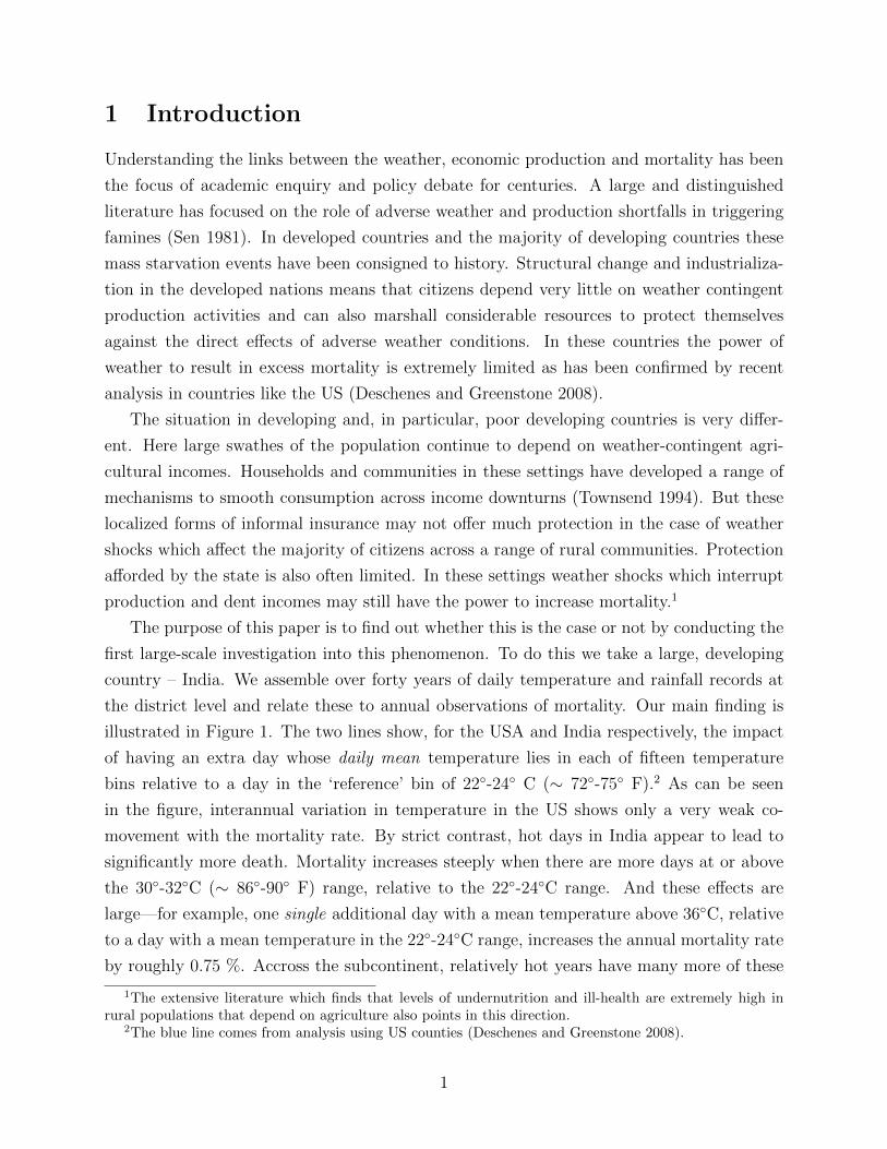
1 Introduction

Understanding the links between the weather, economic production and mortality has been

the focus of academic enquiry and policy debate for centuries. A large and distinguished

literature has focused on the role of adverse weather and production shortfalls in triggering

famines (Sen 1981). In developed countries and the majority of developing countries these

mass starvation events have been consigned to history. Structural change and industrializa-

tion in the developed nations means that citizens depend very little on weather contingent

production activities and can also marshall considerable resources to protect themselves

against the direct effects of adverse weather conditions. In these countries the power of

weather to result in excess mortality is extremely limited as has been confirmed by recent

analysis in countries like the US (Deschenes and Greenstone 2008).

The situation in developing and, in particular, poor developing countries is very differ-

ent. Here large swathes of the population continue to depend on weather-contingent agri-

cultural incomes. Households and communities in these settings have developed a range of

mechanisms to smooth consumption across income downturns (Townsend 1994). But these

localized forms of informal insurance may not offer much protection in the case of weather

shocks which affect the majority of citizens across a range of rural communities. Protection

afforded by the state is also often limited. In these settings weather shocks which interrupt

production and dent incomes may still have the power to increase mortality.1

The purpose of this paper is to find out whether this is the case or not by conducting the

first large-scale investigation into this phenomenon. To do this we take a large, developing

country – India. We assemble over forty years of daily temperature and rainfall records at

the district level and relate these to annual observations of mortality. Our main finding is

illustrated in Figure 1. The two lines show, for the USA and India respectively, the impact

of having an extra day whose daily mean temperature lies in each of fifteen temperature

bins relative to a day in the ‘reference’ bin of 22◦-24◦ C (∼ 72◦-75◦ F).2 As can be seen

in the figure, interannual variation in temperature in the US shows only a very weak co-

movement with the mortality rate. By strict contrast, hot days in India appear to lead to

significantly more death. Mortality increases steeply when there are more days at or above

the 30◦-32◦C (∼ 86◦-90◦ F) range, relative to the 22◦-24◦C range. And these effects are

large—for example, one single additional day with a mean temperature above 36◦C, relative

to a day with a mean temperature in the 22◦-24◦C range, increases the annual mortality rate

by roughly 0.75 %. Accross the subcontinent, relatively hot years have many more of these

1The extensive literature which finds that levels of undernutrition and ill-health are extremely high inrural populations that depend on agriculture also points in this direction.

2The blue line comes from analysis using US counties (Deschenes and Greenstone 2008).

1

lethal days, as we detail below.

Put simply, hot weather is a major source of excess mortality in India but not in the US.

To better understand why this is the case we first split out mortality observations into those

observed for rural and urban populations of Indian districts. This allows us to understand

whether or not the weather-death relationship is different for populations that are more or

less dependent on weather contingent forms of economic production. The high frequency

of our weather data also allows us to examine if weather during the growing season affects

mortality differently from weather in the non-growing season. We also gather data on output,

wages and prices for both urban and rural parts of districts in order to dig into the channels

via which weather might affect death.

The results we uncover suggest weather in India kills by denting agricultural incomes

via the interruptions it imposes on agricultural production and employment. We observe no

effect of weather on death in urban areas of India. This is true even for infants. All the effects

we observe in Figure 1 are coming through effects in rural areas. And it is only the weather

in the growing season that leads to higher death rates despite the fact that the non-growing

season in India is the hottest period of the year. Finally hot weather is associated with low

agricultural yields, lower agricultural wages and higher agricultural prices. Yields and wages

exhibit a pattern which is the inverse of that shown in Figure 1 where having more days

at or above the 30◦-32◦ C range (relative to 22◦-24◦C) is associated with significantly lower

wages and yields. These results suggest that weather variation plays an important role in

the economic lives and health status of India’s rural citizens.

An important finding from the paper is that the structure of production and employment

mediates the impact of weather on death. This is the motivation for looking seperately at

effects on rural and urban populations in the same Indian district and at the effects of

weather during the growing and non-growing seasons in rural areas. In our analysis rural

and urban populations experience the same weather. However, it is only in the former that

we see downturns in output, incomes, wages and increases in prices. And moreover, these

effects are only the result of weather during the growing season. And it is inclement weather

precisely during this period that is driving up mortality in rural but not urban populations

within districts. Weather during the non-growing season which is the hottest, driest part of

the year does not affect mortality in either rural or urban areas. Thus though much of the

literature in developed countries has focussed on heat stress leading to excess mortality our

results suggest that agricultural incomes represent a key channel via which hot weather (and

deficient rainfall) affects death in poor, developing countries like India.

Our results match well with an extensive development literature on lean or hungry seasons

(Khandker 2009). This literature documents that malnutrition and morbidity are highest

2

in the run-up to the post-monsoon harvest when food stocks are depleted, demand for

labor and agricultural wages are low, and food prices are high. Abnormally hot weather

during this period (particularly days above the 32◦-34◦ C) limit the formation of grains in

key crops such as rice and therefore negatively affects the sizes of harvest and accentuate

income downturns for those dependent on agriculture. These effects are magnfied if rainfall

is also scant. Therefore hot weather (and deficient rainfall) can be particularly damaging

for agricultural incomes, wages and prices during the post-monsoon growing season which is

precisely what we find in our data. A variety of behaviours have evolved to deal with weather

shocks during the lean season – running down food stocks and other assets (e.g. savings,

livestock), borrowing money, forward selling labor and migrating have all been documented

in the literature. But our results suggest that the poorest, rural residents (e.g. landless

laborers) may be unable to fully withstand these income shocks and and as a result excess

mortalty results. And morevoer the mortality effects of growing season weather shocks

appear to persistent in the sense that abnormally hot weather in previous years’ growing

seasons adversely affects mortality in the current year though this effect dies out over time.

Famines may have indeed come to an end in India. However, our results suggest that

citizens or rural India still live in a world where inclement weather can significantly elevate

mortality. The fact that the weather may become more inclement via global warming is

then likely to pose particular challenges in these poor, rural settings. In a final section of

this paper we use our estimated coefficients of the within-sample (1957-2000) temperature-

death relationship in India to investigate the mortality predictions implied by two leading

climatological models of climate change. Our within-sample mortality estimates suggest

an increase in the overall Indian annual mortality rate of approximately 12% to 46% by

the end of the century. The estimated increase in rural areas ranges between 21% and

62%. As a reference point, a similar exercise performed on the United States suggests that

climate change will lead to a roughly 2% increase in the mortality rate there by the end of

the century. We fully expect rural Indians to adapt to an anticipated and slowly warming

climate in various ways and so these should be viewed as upper bound estimates. But the

direction of travel is nonetheless worrying and the fact that rural Indian citizens are already

not fully protected from the effects of weather implies that much more careful thinking has to

be applied to understanding how such protection might be afforded. And our results suggest

that calls for workable solutions are likely to need to become more urgent and strident as

global warming proceeds.

The remainder of this paper proceeds as follows. The next section outlines a theoretical

framework that describes the mechanisms through which weather might be expected to

lead to death. Section 3 describes the background features of India in our sample period

3

from 1957-2000, as well as the data on weather, death and economic variables that we

have collected in order to conduct our analysis. Section 4 outlines our empirical method.

Section 5 presents results of the weather-death and weather-income relationships. Section

6 discusses what these estimates imply for predicted climate change scenarios in India, and

finally Section 7 concludes.

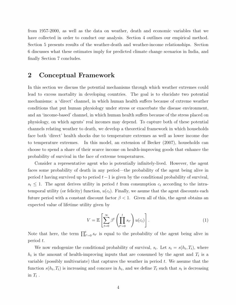
2 Conceptual Framework

In this section we discuss the potential mechanisms through which weather extremes could

lead to excess mortality in developing countries. The goal is to elucidate two potential

mechanisms: a ‘direct’ channel, in which human health suffers because of extreme weather

conditions that put human physiology under stress or exacerbate the disease environment,

and an ‘income-based’ channel, in which human health suffers because of the stress placed on

physiology, on which agents’ real incomes may depend. To capture both of these potential

channels relating weather to death, we develop a theoretical framework in which households

face both ‘direct’ health shocks due to temperature extremes as well as lower income due

to temperature extremes. In this model, an extension of Becker (2007), households can

choose to spend a share of their scarce income on health-improving goods that enhance the

probability of survival in the face of extreme temperatures.

Consider a representative agent who is potentially infinitely-lived. However, the agent

faces some probability of death in any period—the probability of the agent being alive in

period t having survived up to period t−1 is given by the conditional probability of survival,

st ≤ 1. The agent derives utility in period t from consumption ct according to the intra-

temporal utility (or felicity) function, u(ct). Finally, we asume that the agent discounts each

future period with a constant discount factor β < 1. Given all of this, the agent obtains an

expected value of lifetime utility given by

V = E

[∞∑t=0

βt

(t∏

t′=0

st′

)u(ct)

]. (1)

Note that here, the term∏t

t′=0 st′ is equal to the probability of the agent being alive in

period t.

We now endogenize the conditional probability of survival, st. Let st = s(ht, Tt), where

ht is the amount of health-improving inputs that are consumed by the agent and Tt is a

variable (possibly multivariate) that captures the weather in period t. We assume that the

function s(ht, Tt) is increasing and concave in ht, and we define Tt such that st is decreasing

in Tt .

4

Crucial to this framework is the assumption that ht is a choice variable that is under the

agent’s control (subject to a budget constraint). Note that, in this formulation, there are

two types of goods. Consumption goods (denoted by ct) are goods that the agent values

directly—they enhance the agent’s quality of life and are the sole argument in the utility

function, u(ct). Health input goods (denoted by ht) are valued only because they improve

the likelihood of survival in the current period and in future periods. We provide some

examples of health input goods, especially those that are important in our context, below.

The fact that the weather Tt affects that conditional probability of survival directly

(ie st = s(ht, Tt)) allows for the direct effect relating weather to mortality. The weather

Tt is assumed to be out of the agent’s control. Holding health inputs ht constant, high

temperatures can cause death (decrease survival chances st) directly. An extensive public

health literature discusses the potential direct effects of high temperatures on human health

(see, for example, Basu and Samet (2002) for a comprehensive review).3 Periods of excess

temperature place additional stress on cardiovascular and respiratory systems due to the

demands of body temperature regulation. This stress is known to impact on the elderly and

the very young with particular severity, and can, in extreme cases, lead to death (Klineberg

2002, Huynen, Martents, Schram, Weijenberg, and Kunst 2001). An alternative ‘direct’ effect

of extreme weathers on death in India could include the possibility that disease pathogens

(for example, diarrhoeal diseases) thrive in hot and wet conditions, or that some vectors

of disease transmission (such as mosquitoes in the case of malaria) thrive in hot and wet

environments. We collapse all of these potential ‘direct’ channels into the possibility that

some index of temperature Tt enters the function s(ht, Tt) directly (and negatively).

To allow for an ‘income-based channel’ through which weather extremes can cause death,

we include the possibility that the agent’s income is a function of the weather: yt = y(Tt).

This is extremely likely in rural areas where incomes depend on agriculture directly or

indirectly. For simplicity, we assume that the weather variable Tt potentially affects both

income and survival in the same direction, such that y is decreasing in T . Because incomes are

observable the weather-to-income relationship is one that we are able to estimate. Naturally,

we expect this relationship to be minimal or even absent in urban areas. In contrast,

following well-known effects in the agronomic literature, as well as the literature on expected

effects of hotter climates on Indian agriculture (eg Kumar, Kumar, Ashrit, Deshpande,

and Hansen (2004) and Guiteras (2008)), we expect a strong negative relationship between

3Extremely cold temperatures can also affect human health adversely through cardiovascular stress dueto vasoconstriction and increased blood viscosity. Deschnes and Moretti (2009) find evidence for a moderateeffect of extreme cold days on mortality (especially among the elderly) in the United States, though thiseffect is concentrated among days below 10◦ F (ie −12◦ C). Days in this temperature range are extremelyrare in India.

5

incomes in rural areas (ie agricultural incomes) and temperatures.

An income shortage caused by weather extremes could lead to death if this shortage

forces the agent to cut back on health input goods, ht. We take a broad view of these health

input goods, which the poor may struggle to afford even at the best of times, nevermind

those periods when weather extremes have caused income shortages. These could include

traditional health goods such as medicine or visits to a health center. Equally, they could

include the subsistence component of food consumption (that which increases the likelihood

of survival but is not valued in u(c) directly). Or given our focus on temperature an important

‘health good’ might be the use of air conditioning. More broadly, this ‘health good’ could

also encompass any leisure or rest (ie foregone labor, or income-earning opportunities) that

the agent might decide to ‘purchase’ so as to improve his health. This could include the

decision to work indoors rather than outdoors when it is hot, or to accept an inferior paying

job so as to avoid working outside on a hot day.

Finally, we specify the timing through which the uncertainty is resolved through time.

At the beginning of a period (for example, period t = 0), the temperature in the current

period (eg T0) is drawn. The agent then makes his choices in the current period (ie c0 and

h0) as a function of the current temperature (ie c0 = c0(T0) and h0 = h0(T0)). After the

agent’s decision has been made, the agent’s death shock arrives (ie, having survived up to

date 0, the agent survives with probability s0 = s(h0, T0).) Finally, if the agent survives this

death shock he enjoys intra-period utility u(c0) and the next period begins. If the agent

dies in period 0 then he enjoys no utility from this period (though the assumption of zero

utility in death is merely a normalization).

We specify the agent’s budget constraint as follows. We assume that the price of the

consumption good ct is pc and that of the health input good ht is ph; this relative price

governs intra-temporal decisions. For simplicity we assume these prices are constant over

time. We also assume, for simplicity, that agents are able to borrow or save across periods

at the interest rate r (which is assumed to be constant, for simplicity) and that the agent

has access to a complete and fair annuity market (the only role of which is to simplify the

presentation of the lifetime budget constraint by ruling out the possibility that the agent

lives longer than expected and runs out of resources, or that the agent dies early when in

debt).

Under the above assumptions the agent’s inter-temporal budget constraint, starting from

period 0, can be written as:

s0[y(T0)− pcc0 − phh0] = E

[∞∑t=1

R−t

(t∏

t′=0

st′

)(pcct + phht − y(Tt))

], (2)

6

where R = (1 + r). That is, if total expenditure in period 0 (ie pcc0 + phh0) exceeds income

in period 0, y(T0), then this must be funded by future surpluses.

An agent who maximizes lifetime utility, equation (1), subject to his lifetime budget con-

straint, equation (2), from the perspective of period 0 after T0 is known will make choices that

satisfy the following necessary first-order conditions for optimization. First, his allocation

of consumption across time will satisfy a standard Euler equation:

u′(c0) =βRE [s1u

′(c1)]

E[s1].

This result states that the marginal utility of consumption in period 0 will be equal to the

expected marginal utility of consumption in the next period, times the opportunity cost

of consumption in the next period. This is the standard Euler equation adjusted for the

fact that the marginal utility of consumption in period 1 (ie u′(c1)) will only bring utility

if the agent survives (ie s1 = 1), and adjusted also for the fact that opportunity cost of

consumption in period 0 is also reduced by the possibility of non-survial (ie s1 <= 1).

Second, the choice of the health input good in period 0, h0, will satisfy the following

first-order equation

∂s0∂h

[u(c0) + E

[∞∑t=1

βt

(t∏

t′=1

st′

)u(ct)

]]= λphs0,

where λ is the marginal utility of lifetime income (in terms of the numeraire, the health input

good). In what follows we will find it useful to define E[V0] = u(c0)+E[∑∞

t=1 βt(∏t

t′=1 st′)u(ct)

]as the expected utility of surviving the death shock (that is, of being alive) in period 0. If

the agent is alive in period 0 then he enjoys both consumption this period (ie u(c0)) and

the possibility of being alive in the future to enjoy utility from consumption then. This

first-order equation for the choice of h0 can therefore be written as

∂s0∂h

E[V0]

λs0= ph.

In this formulation, the term E[V0]λs0

is the agent’s ‘value of a statistical life’ (VSL). This is

the value (in monetary units) of being alive at the start of date 0. The first-order condition

therefore states that, at the optimal choice, the marginal benefit of spending more money

on the health input (which is given by the product of the effect that the health input has

on survival, ∂s0∂h

, and the value of survival, the VSL) equals the marginal cost of spending

money on the health input (given simply by the price of the health input, ph).

Finally, by studying the agent’s expected choice of the health input in period 1, h1, one

7

can derive an equation for the change in health spending across periods 0 and 1 which is

analogous to the consumption Euler equation presented above. This health input Euler

equation is:

E[∂s0∂h

V0λs0

]= βRE

[∂s1∂h

V1s1λ

1 + ∂s1∂h

W1

s1

]. (3)

Here, V1 is the value of being alive at the start of period 1, and W1 is the agent’s net

asset position at the start of period 1. To gain intuition for this equation, imagine that the

agent’s net asset position at the start of period 1 is zero (ie W1 = 0), just as it was (by

normalization) at the start of period 0. In such a setting, this health input Euler equation is

entirely analogous to the consumption Euler equation introduced earlier: up to the dynamic

adjustment factor βR (which trades off the agent’s taste for impatience β with the returns to

saving R), the agent tries to equalize the expected marginal value of health spending across

periods. Since the maginal value of health spending is given by the product of the marginal

effect of health saving on survival ( ∂s∂h

) and the value of survival (the VSL, Vsλ

), the result in

equation (3) follows. More generally, W1 may not equal zero. But this simply adjusts the

above intuition for the fact that the agent does not want to risk dying with assets unspent.

This last result, the health spending Euler equation in equation (3), suggests that we

should expect a great deal of smoothing, not only in health expenditure but also in the

probability of survival itself. For a potentially long lived agent, the value of life at date 0

should be close to that at date 1, as long as the probability of death is being smoothed over

time. And since (by assumption) the marginal effect of health expenditure on survival ( ∂s∂h

)

is strictly decreasing in h, equation (3) suggests that we should expect the agent to be trying

to smooth (again, up to the adjustment factor βR) expected health expenditures h as well

as the expected value of life.

A final implication of the above first-order conditions is that they can be used to charac-

terize the agent’s willingness to pay (WTP) to avoid a worsening in the weather (∆T0 > 0)

in period 0. One way to derive the WTP is to imagine a transfer that varies as a function

of the observed weather T0 in period 0 and is designed to hold expected lifetime income V

constant for any value of T0. Denote this transfer y∗(T0). It is then straightforward to show

that this transfer scheme will vary with T0 in the following manner:

dy∗(T0)

dT0= −dy(T0)

dT0+∂h0∂T0− ds(h0, T0)

dT0E[V0s0λ

]. (4)

This expression, which characterizes the agent’s willingness to pay to avoid a small wors-

ening in the weather dT0, is intuitive. WTP is the sum of three terms in this model. First,

since weather increases may adversely affect incomes directly (the ‘income-based channel’)

8

the WTP first requires compensation for any loss of income caused by worse weather (ie a

payment of −dy(T0)dT0

, which we expect to be positive if bad weather leads to lower incomes).

Second, since inclement weather causes the agent to spend resources on health inputs that

have no direct utility benefits, the WTP requires the agent to be compensated for any change

in expenditures on health inputs caused by the worsening in the weather (ie a payment of∂h0∂T0

, which we expect to be positive if there is a direct effect of weather extremes on survival

chances that the agent is attempting to offset through the purchase of the heath good). The

final term in this WTP expression compensates the agent for the heightened risk of death

caused by inclement weather. Such a compensation requires a payment of −ds(h0,T0)dT0

E[V0s0λ

],

which is the product of the total effect of weather extremes on survival chances (ie ds(h0,T0)dT0

)

and the dollar value of survival in period 0, E[V0s0λ

], often referred to as the ‘value of a

statistical life’. The fact that this expression depends on the total deriviative of survival

with respect to weather, ds(h0,T0)dT0

, rather than the partial deriviative holding the health input

constant, is attractive from an empirical perspective.

It is important to note that all of the terms in the WTP expression in equation (4) are

potentially observable. Our empirical analysis below will aim to estimate both the the

reduced-form (or ‘total’) effect of weather extremes on death, ie ds(h0,T0)dT0

, and the effect of

weather extremes on income, ie dy(T0)dT0

. Armed with these two essential ingredients and an

estimate of the value of a statistical life in our setting (ie E[V0s0λ

]) we will therefore be able

to estimate a lower bound on the agent’s willingness to pay to avoid a small worsening of

the weather, dT0. This estimate will be a lower bound on the WTP because of our inability

to observe the full vector of health inputs that households are purchasing, and hence our

inability to estimate ∂h0∂T0

.

An important lesson from the WTP expression in equation (4) is that, in this model,

because money is fungible, it is irrelevant whether the agent suffers a heightened risk of

death due to weather extremes because of a ‘direct’ effect of bad weather on death or an

‘income-based’ effect. In either case, the agent has a well-defined willingness to pay to avoid

a inclement weather that is given by our WTP expression. This fact informs our empirical

approach which is centered on estimating two important ingredients that are required to

obtain bounds on the agent’s WTP, the reduced-form effect of weather on death (ie ds(h0,T0)dT0

)

and the effect of weather on incomes (ie dy(T0)dT0

).

We conclude with a final word about policy in this environment. There are no market

failures in the above model—though it is clearly easy to imagine extensions to the model that

would involve plausible market failures, most notably constraints on the ability of agents to

borrow across periods without any restraint other than the inter-temporal budget constraint.

The absence of market failures implies no role for a self-funded policy here—a policy-maker

9

facing the same constraints as the agent could do no better than the agent is doing himself.

But the WTP expression above does characterize the value that households place on avoiding

temperature extremes, which an external funder, such as a foreign donor, might wish to use

to compare the merits of competing policy proposals.

3 Background and Data

To implement the analysis in this paper, we have collected the most detailed and compre-

hensive district-level data available from India on the variables that the above conceptual

framework in Section 2 suggests are important. These variables include demographic vari-

ables (population, mortality and births), and variables that capture key features of India’s

urban and rural economies (output, prices and wages). We then study the relationship be-

tween these data and high-frequency daily data on historical weather that we have assembled.

In this section we describe these data, their summary statistics, and the essential features of

the background economy they describe.

Throughout this paper we draw heavily on the implications of the differential weather-

death relationship in urban and rural areas. We therefore begin with a short discussion of the

essential differences between these regions. Despite the dramatic extent to which the world

has urbanized in the last sixty years, the extent of urbanization in India has been relatively

slow: even in 2001, 72.2 percent of Indians lived in rural areas. The overriding distinction

between economic life in rural and urban India is the source of residents’ incomes. 76 % of

rural citizens belong to households that draw their primary incomes from employment in the

agricultural sector, while only 7 % of those in urban areas do so. Another distinction between

rural and urban areas lies in their consumption of food—that is, in their exposure to fluc-

tuations in the prices of foodstuffs. Deaton and Dreze (2009) draw on consumption surveys

to report that in 2001, 58 % of the average rural residents’ budget was spent on food, while

only 45 % of the average urban budget was devoted to food. Naturally, these consumption

differences may represent differences in the level of household per capita incomes between

rural and urban areas. Urban households are, on average, richer than rural households: in

2001 urban residents were 69 % richer on average than rural residents, according to Deaton

and Dreze (2009).

3.1 Data on Mortality and Population

The cornerstone of the analysis in this paper is district mortality data taken from the Vital

Statistics of India (VSI) publications for 1957-2000, which were digitized for this project.

10

The VSI data represent the universe of registered deaths in each year and registration was

compulsory in India throughout our sample period. This source contains the most detailed

possible panel of district-level mortality for all Indian citizens.

Death tallies in the VSI are presented for infants (deaths under the age of one) and for

all others (deaths over the age of one), by rural and urban areas separately.4 From this

information we construct two measures of mortality: an infant mortality rate, defined as the

number of deaths under the age of one per 1000 live births; and an ‘all ages’ mortality rate,

defined as the total number of deaths over the age of one normalized by the population in

1000s.

Table 1 (which contains all of the summary statistics for data used in this paper) sum-

marizes the VSI data from the 1957-2000 period that we use in this paper, which comprise

315 districts spanning 15 of India’s largest states (and account for over 85 % of India’s pop-

ulation).5 The table reveals that measured mortality rates are high throughout this period.

For example, the average infant mortality rate is 40.5 per 1,000 live births. Geographi-

cally, average infant mortality rates range from 17.7 per 1,000 in Kerala to 71.3 per 1,000

in Orissa, revealing the substantial heterogeneity. As a basis of comparison, the mean US

infant mortality rate over these years was roughly 12 per 1,000. The Indian overall mortality

rate was 6.6 per 1,000. It is important to stress that these mortality rates are almost surely

underestimates of the extent of mortality in India. Despite compulsory registration of births

and deaths, many areas of the country suffer from significant under-reporting.6

Table 1 also documents the time variation in the two mortality rates. There is a remark-

able decline in both mortality rates in both rural and urban regions. For example, the overall

mortality rate declines from roughly 12 in 1957 to about 4 in rural areas and 6 in urban

areas by 2000. The decline in the infant mortality rate is also impressive, going from about

100 per 1,000 in 1957 to roughly 13.5 per 1,000 in 2000. In Section 4 below, we describe

our strategy to avoid confounding these trends in mortality rates with any time trends in

4The rural/urban assignment is based on the following criteria, used throughout official Indian statistics:urban areas comprise “(a) all places with a Municipality, Corporation or Cantonment or Notified Town Area;and (b) all other places which satisfied the following criteria: (i) a minimum population of 5,000, (ii) at least75% of the male working population was non-agricultural, and (iii) a density of population of at least 400per sq. Km. (i.e. 1000 per sq. Mile).”

5These states are (in 1961 borders and names): Andhra Pradesh, Bihar, Gujarat, Himachal Pradesh,Jammu and Kashmir, Kerala, Madhya Pradesh, Madras, Maharashtra, Mysore, Orissa, Punjab, Rajasthan,Uttar Pradesh, and West Bengal. These are the states with a consistent time series of observations in theVSI data. The results in this paper are largely insensitive to the inclusion of all observations in the VSIdata.

6According to the National Commission on Population of India, only 55 % of the births and 46 % of thedeaths were being registered in 2000. These estimates were obtained from India’s Sample Registration Sys-tem, which administers an annual survey of vital events to a nationally representative sample of households.The data published by the SRS, however, are only available at the state level.

11

temperatures.

3.2 Data on Weather

A key finding from Deschenes and Greenstone (2008) is that a careful analysis of the relation-

ship between mortality and temperature requires daily temperature data. This is because

the relationship between mortality and temperature is highly nonlinear and the nonlinear-

ities would be missed with annual or even monthly temperature averages. This message is

echoed in the agronomic and agricultural economics literatures (as emphasized, for example,

by Deschenes and Greenstone (2007) and Schlenker and Roberts (2008)).

Although India has a system of thousands of weather stations with daily readings dating

back to the 19th century, the geographic coverage of stations that report publicly available

temperature readings is poor (and surprisingly the public availability of data from these

stations drops precipitously after 1970). Further, there are many missing values in the

publicly available series so the application of a selection rule that requires observations from

365 days out of the year would yield a database with very few observations.

As a solution, we follow Guiteras (2008) and use data from a gridded daily dataset that

uses non-public data and sophisticated climate models to construct daily temperature and

precipitation records for 1◦ (latitude) × 1◦ (longitude) grid points (excluding ocean sites).

This data set, called NCC (NCEP/NCAR Corrected by CRU), is produced by the Climactic

Research Unit, the National Center for Environmental Prediction / National Center for

Atmospheric Research and the Laboratoire de Meteorologie Dynamique, CNRS. These data

provide a complete record for daily average temperatures and total precipitation for the

period 1950-2000. We match these gridpoints to each of the districts in our sample by

taking weighted averages of the daily mean temperature and total precipitation variables

for all grid points within 100 KM of each district’s geographic center. The weights are the

inverse of the squared distance from the district center.7

To capture the distribution of daily temperature variation within a year, we use two

different variables. The first of these temperature variables assigns each district’s daily

mean temperature realization to one of fifteen temperature categories—as already seen in

Figure 1. These categories are defined to include daily mean temperature less than 10◦ C

(50◦ F), greater than 36◦ C (96.8◦ F), and the thirteen 2◦ C-wide bins in between. The 365

7On average, there are 1.9 grid points within a 100 km radius circles. The subsequent results are insensitiveto taking weighted averages across grid points across distances longer than 100 km and using alternativeweights (e.g., the distance, rather than the squared distance). After the inverse distance weighting procedure,339 out of a possible 342 districts have a complete weather data record. The three districts that are droppedin this procedure are Alleppey (Kerala), Laccadive, Minicoy, and Amindivi Islands, and the Nicobar andAndaman Islands.

12

daily weather realizations within a year are then distributed over these fifteen bins. This

binning of the data preserves the daily variation in temperatures, which is an improvement

over previous research on the relationship between weather and death that obscures much

of the variation in temperature.

Figure 2 illustrates the average variation in daily temperature readings across the fifteen

temperature categories or bins over the 1957-2000 period. The height of each bar corresponds

to the mean number of days that the average person in the vital statistics data (described

below) experiences in each bin; this is calculated as the weighted average across district-by-

year realizations, where the district-by-year’s total population is the weight. The average

number of days in the modal bin of 26◦-28◦ C is 72.9. The mean number of days at the

endpoints is 3.7 for the less than 10◦ C bin and 3.4 for the greater than 36◦ C bin.

As a second approach to capturing the influence of temperature, we draw on a stark

non-linearity in the relationship between daily temperatures and both human and plant

physiology that is well known in the public health and agronomy literatures: temperatures

above (approximately) 32◦ C are particularly severe. We therefore construct a measure

of the cumulative number of degrees-times-days that exceed 32◦ C in a district and year.

This ‘degree-days’ measure has the advantage of collapsing a year’s 365 daily temperature

readings down to one single index, while still doing some justice to what is known about the

non-linear effects of temperature. Table 1 reports on summary statistics of this measure.

The national average is approximately 65 degree-days per year over 32◦ C, which implies an

average of just over two months during the year in which the daily mean temperature is at

34◦ C.

While the primary focus of our study is the effect of high temperatures on mortality,

we use data on rainfall to control for this potential confounding variable (to the extent

that temperature and rainfall are correlated). Table 1 reports annual precipitation totals.

However, the striking feature of rainfall in India is its intra-annual distribution: in an average

location, over 95 percent of annual rainfall arrives after the arrival of the southwest (summer)

monsoon, a stark arrival of rain on the southern tip of the subcontinent around June 1st which

then moves slowly northwards such that the northern-most region of India experiences the

arrival of the monsoon by the start of July—see, for example, Wang (2006). Naturally this

stark arrival of rainfall after a period of dryness triggers the start of the agricultural season

in India. We exploit this feature of the timing in our analysis below.

13

3.3 Data on Economic Outcomes in Rural India

3.3.1 Agricultural Yields

It is natural to expect that the weather plays an important role in the agricultural economy

in India. In turn, the agricultural economy may play an important role in the health of rural

citizens who draw their incomes from agriculture. To shed light on these relationships we

draw on the best available district-level agricultural data in India. The data on agricultural

outputs, prices, wages, and employment come from the ‘India Agriculture and Climate Data

Set’, which was prepared by the World Bank.8 This file contains detailed district-level data

from the Indian Ministry of Agriculture and other official sources from 1956 to 1986. From

this source we utilize three distinct variables on the agricultural economy: yields, prices, and

wages.

We construct a measure of annual, district-level yields by aggregating over the output

of each of the 27 crops covered in the World Bank dataset (these crops accounted for over

95 percent of agricultural output in 1986). To do this we first create a measure of real

agricultural output for each year (using the price index discussed below) and then divide

this by the total amount of cultivated area in the district-year. Table 1 reports on the

resulting yield measure for the 271 districts contained in the World Bank dataset, over the

period from 1956 to 1987. All of the major agricultural states are included in the database,

with the exceptions of Kerala and Assam.

3.3.2 Agricultural Prices

Because rural households spend so much of their budgets on food, food prices are an im-

portant determinant of rural welfare in India. We construct an agricultural price index for

each district and year which attempts to provide a simple proxy for the real cost of pur-

chasing food in each district-year relative to a base year. Our simple price index weights

each crop’s price (across the 27 crops in the World Bank sample) by the average value of

district output of that crop over the period.9 Table 1 reports on the level of this price index

in rural India. (The price data used in the World Bank source are ‘farm harvest prices’, so

we prefer to interpret these as rural prices rather than urban prices.) These figures and their

accompanying standard deviations show that prices are not as variable over space and time

as the yield figures in Table 1, potentially reflecting a degree of market integration across

India’s districts (so that a market’s price is determined by supply conditions both locally

8The lead authors are Apurva Sanghi, K.S. Kavi Kumar, and James W. McKinsey, Jr.9Annual, district-level consumption data, which would be required to construct a more appropriate con-

sumption-based price index, are not available in India.

14

and further afield).

3.3.3 Real Agricultural Wages

A second important metric of rural incomes (in addition to agricultural productivity, dis-

cussed above) is the daily wage rate earned by agricultural laborers. The World Bank dataset

contains information on daily wages, as collected by government surveys of randomly chosen

villages in each district and year. All figures are given in nominal wages per day, and are

then converted into equivalent daily rate to reflect the (low) degree of variation in the num-

ber of hours worked per day across the sample villages. We divide the reported, nominal

wage rate by the agricultural price index described above to construct an estimate of the

real rural agricultural wage in each district-year.10 As can be seen in Table 1, the level of

real wages is low throughout the period—never rising above 33.96 Rupees (base year 2000),

or approximately 2 US dollars (base year 2000) per day in PPP terms.

3.4 Data on Economic Outcomes in Urban India

As emphasized in Section 2, an important channel through which weather variation can

reduce welfare and lead to death is through household’s incomes. While it is natural to expect

strong effects of temperature extremes on rural, agricultural incomes, we also investigate the

extent to which economic conditions in urban areas react to temperature fluctuations. To

this end we have collected the best available data on urban economic conditions, and describe

the sources of that data here. It is important to stress at the outset that, perhaps because

of the over-riding current and historical importance of agriculture for economic welfare in

India, the statistics on India’s urban economy are not as detailed as those on India’s rural,

agricultural economy. All of the sources listed below report data on urban outcomes at the

state level, whereas all of the rural equivalents introduced above were available at the district

level.

3.4.1 Manufacturing Productivity

India’s manufacturing sector (especially its ‘registered’ or formal manufacturing sector) is

almost entirely located in urban areas. For this reason we use a measure of state-level

registered manufacturing productivity (real output per worker) as one measure of the pro-

ductivity of the urban area of each state in each year. We draw this data from Besley and

10A better real wage measure would of course also incorporate price information on non-agricultural itemsin the rural consumption basket. Unfortunately, the price and quantity information that would be requiredto do this are unavailable annually at the district level in India.

15

Burgess (2004), who collected the data from publications produced by India’s Annual Survey

of Industries.

3.4.2 Urban Consumer Price Index

Every year India’s statistical agencies produce two official consumer price indices, one in-

tended to be relevant for agricultural workers and one intended to be relevant for manufac-

turing workers. These are published by the Labour Bureau. The latter index is collected

(by the NSSO) from urban locations, and is based on weights drawn from NSS surveys of

manufacturing workers. We therefore follow standard practice and use on the manufacturing

workers’ CPI as a CPI that reflects urban prices. Data on this index is taken from Besley and

Burgess (2004), who collected the data from the annual Indian Labour Yearbook publication.

3.4.3 Real Manufacturing Wages

The final measure of incomes in urban areas that we exploit comes from manufacturing wage

data. To construct this variable we first use data on nominal (registered) manufacturing

wages, as surveyed by the Annual Survey of Industries and published in the annual Indian

Labour Yearbook, which was collected by Besley and Burgess (2004). We then divide nominal

manufacturing wages by the urban CPI variable introduced above to create a measure of

real manufacturing wages.

4 Methodology

In this section we describe the econometric method that we use to analyze the weather-death

relationship and accompanying relationships in this paper.

We pursue two different approaches to modeling the temperature-death relationship, but

our approach to the precipitation-death relationship is held constant throughout. Our first

approach to estimating the temperature-death relationship was introduced briefly in the

Introduction, and results based on it were presented in Figure 1, but we provide details here.

Our estimating equation uses a flexible specification to model the relationship between daily

temperature variation and annual mortality rates as follows:

Ydt =∑j

θ15j=1TMEANdtj +∑k

δk1 {RAINdtin tercile k}

+ αd + γt + λ1rt+ λ2rt2 + εdt, (5)

where Ydt is the log mortality rate (or an alternative outcome variable such as an income

16

measure) in district d in year t. We use the log of the death rate (or of alternative outcome

variables) in order to draw straightforward comparisons across different outcome variables,

but our results are largely unchanged if we instead use the level of the death rate (or alter-

native outcome) rather than its log as our dependent variable. The r subscript refers to a

‘climatic region’ (explained below). The last term in the equation is a stochastic error term,

εdt.

The key variables of interest here are those that capture the variation in daily temper-

atures in district d within year t. The variable TMEANdtj denotes the number of days in

district d and year t on which the daily mean temperature fell in the jth of the fifteen bins

used in Figure 2. We estimate separate coefficients θj for each of these temperature bins.

However, because the number of days in a standardized year always sums to 365 one of these

fifteen coefficients cannot be identified; we use the middle bin, that for temperatures between

22◦ C and 24◦ C, as a reference category whose coefficient is therefore normalized to zero.

This approach makes three assumptions about the effect of a day’s mortality impact

on the outcome variable. First, this approach assumes that the impact is governed by the

daily mean alone; since daily data on the intra-day (‘diurnal’) variation of temperatures in

India over this time period is unavailable to us, this assumption is unavoidable. Second,

our approach assumes that the impact of a day’s mean temperature on the annual mortality

rate is constant within 2◦ C degree intervals; our decision to estimate separate coefficients θj

on each of fifteen temperature bin coefficients represents an effort to allow the data, rather

than parametric assumptions, to determine the mortality-temperature relationship, while

also obtaining estimates that are precise enough that they have empirical content. This

degree of flexibility and freedom from parametric assumptions is only feasible because of the

use of district-level data from 44 years. Finally, by using as a regressor the number of days

in each bin we are assuming that the sequence of relatively hot and cold days is irrelevant for

how hot days affect the annual outcome variable. This is a testable assumption, for which

we find support. Specifically, including regressors that capture the presence of two or more

‘hot’ days (eg over 32◦ C) does not change our main results.

The second set of variables on the right-hand side of equation (5) aims to capture variation

in precipitation (essentially rainfall, given our sample restriction to non-Himalayan India).

Given that our primary focus is on the effects of temperature on death, the coefficients

on rainfall regressors are of secondary importance. However, because it is possible that

temperature variation is correlated with rainfall variation, the inclusion of these rainfall

variables is important. We model rainfall in a manner that is fundamentally different from

our approach to modeling temperature because of one key difference between temperature

and rainfall: rainfall is far more able to be stored (in the soil, in tanks and irrigation systems,

17

and in stagnant water that might breed disease) than is temperature. Given this distinction,

while we have modeled the effect of temperature as the sum over daily impacts, we model

the effect of rainfall as the impact of sums over daily accumulations. The specific approach

pursued in equation (5) above uses regressors that aim to flexibly capture how a given

year’s total annual rainfall affects the outcome variable. To do this as simply as possible we

calculate whether the total amount of rainfall in year t in district d was in the upper, middle

or lower tercile of annual rainfall amounts in district d over all years in our sample; these

are the regressors 1 {RAINdtin tercile k}. We estimate a separate coefficient on each of the

three tercile regressors (though of course one of these regressors is omitted as a reference

category, which we take to be the middle tercile regressor).

The specification in equation (5) also includes a full set of district fixed effects, αd, which

absorb all unobserved district-specific time invariant determinants of the log mortality rate.

So, for example, permanent differences in the supply of medical facilities will not confound

the weather variables. The equation also includes unrestricted year effects, γt. These fixed

effects control for time-varying differences in the dependent variable that are common across

districts (for example, changes in health related to the 1991 economic reforms). The as-

sumption that shocks or time-varying factors that affect health are common across districts

is unlikely to be valid. Consequently, equation (5) includes separate quadratic time trends

for each of the five climatic regions r of India (groupings of states with similar climates

according to India’s Meteorological Department.)

Our second approach to modeling the temperature-death relationship estimates fewer

parameters while still doing some justice to the non-linear nature of this relationship. This

second approach, which we refer to as the ‘single-index’ approach, estimates the parameters

in:

Ydt = βCDD32dt +3∑

k=1

δk1 {RAINdtin tercile k}+ αd + γt + λ1rt+ λ2rt2 + εdt, (6)

where the variable CDD32dt is the number of cumulative degree-days in district d and year

t that exceeded 32◦ C.11 This is a particular restriction on the flexible approach in equation

(5)—where the 13 temperature bin coefficients θj below 32◦ C are restricted to be zero and

the three coefficients above 32◦ C are restricted to be linearly increasing in their average

temperatures—for which we find some support below.

Our assumptions in pursuing this simplification are that: (i) on days during which the

mean temperature is below 32◦ C, temperature is irrelevant for determining the outcome

11For example, if a given district-year had only two days over 32◦ C, one at 34◦ C and the other at 36◦ C,its value of CDD32dt would be 6.

18

variable (eg mortality) Ydt; and (ii), the effect of days whose mean temperatures exceed 32◦

C is linearly increasing (at the rate β) in the mean daily temperature. This is broadly in

line with a large public health and agronomy literature that uses the cumulative degree-day

approach. The advantage of this single-index approach is that by estimating one coefficient

rather than 15 we have more statistical power for teasing out the heterogeneous effects of

temperature in order to learn more about the weather-death relationship.

The validity of this paper’s empirical exercise rests crucially on the assumption that

the estimation of equations (5) and (6) will produce unbiased estimates of the θj, β and

δk parameters. By conditioning on district fixed effects, year fixed effects, and quadratic

polynomial time trends specific to each climatic region, these parameters are identified from

district-specific deviations in weather about the district averages after controlling for the por-

tion of shocks that remains after adjustment for the year effects and cubic time polynomials.

Due to the randomness and unpredictability of weather fluctuations, it seems reasonable to

presume that this variation is orthogonal to unobserved determinants of mortality rates.

There are two further points about estimating equations (5) and (6) that bear noting.

First, it is likely that the error terms are correlated within districts over time. Consequently,

the paper reports standard errors that allow for heteroskedasticity of an unspecified form

and that are clustered at the district level. Second, we fit weighted versions of equations

(5) and (6), where the weight is the square root of the population in the district for two

complementary reasons.12 First, the estimates of mortality rates from large population

counties are more precise, so this weighting corrects for heteroskedasticity associated with

these differences in precision. Second, the results reveal the impact on the average person,

rather than on the average district, which we believe to be more meaningful.

5 Results

5.1 Weather and Death

Figure 1 in the Introduction of this paper displayed the result of running a regression of

weather on death for India and the US. The two lines in Figure 1 show the impact of

having an extra day in fifteen temperature bins relative to a day in the 22◦-24◦ C bin

for the US and India respectively. That is, the fifteen coefficient estimates θj for each of

fifteen temperature bins j from estimating equation (5) are presented graphically, under the

normalization that coefficient on the middle bin, the 22◦-24◦ C bin, is zero. Further, as

12When estimating relationships in which the outcome variable concerns agricultural income we weight bythe cultivated area of the district-year since the fundamental sampling unit in the data used to constructthese outcome variables is a parcel of land.

19

discussed in Section 4, while only the coefficients on these fifteen temperature regressors are

plotted, these coefficients were estimated while controlling for rainfall variation, district and

year fixed effects, and quadratic polynomial trends for each climatological region. This is

also true for all further graphical presentations of estimates of equation (5) shown below, in

Figures 3 to 5.

As can be seen in Figure 1, interannual variation in temperature in the US shows no clear

relationship with mortality. In strict contrast having more hot days in India is associated

with significantly more death. Mortality increases steeply when there are more days at or

above the 30◦-32◦ C range (relative to 22◦-24◦ C). And the effects are large, for example,

one additional day with a mean temperature above 36◦ C, relative to a day with a mean

temperature in the 22◦-24◦ C range, increases the annual mortality rate by roughly 0.75 %.

Put simply, hot weather kills in India but not—at least on nowhere near the same scale—in

the US.

To better understand why this is the case we first split out mortality observations into

those observed separately for the rural and urban populations of each Indian district. This

allows us to understand whether or not the weather-death relationship is different for popu-

lations that are more or less dependent on weather contigent forms of economic production.

The high frequency of our weather data also allows us to examine if weather during the

growing season affects mortality differently from weather in the non-growing season.

5.1.1 Urban versus Rural

In terms of economic structure, urban and rural India look very different. In employment

terms the rural areas of India are dominated by agriculture whilst urban areas are dominated

by services and manufacturing. As we have seperate observations of mortality for rural

and urban populations within the same district we can test whether the weather-death

relationship differs for these two populations.

The results from doing this are shown in Figures 3 and 4. These figures plot estimated

response functions between log annual mortality rate and temperature exposure, estimated

separately for urban and rural populations. These models pool across age groups and pertain

to the total population of a particular area within each district (i.e. the urban or rural

segment of a district).

Figure 3 shows the response function estimated from the urban population. For both the

urban Indian population and the US population there is, in effect, no significant relationship

between weather and death. The results are remarkably different from those in the rural

areas. The largest urban India coefficient is for the highest temperature bin (> 36◦ C), and

the magnitude is only 0.003—half the magnitude of the all-India coefficient (of 0.075) in

20

Figure 1. Further, it is notable that none of the other temperature effects is statistically

significant, and all are relatively small in magnitude. Figure 4 shows the rural response

function. This plot shows a significant and increasing relationship between log mortality

rates and temperature. The largest coefficient is for the highest temperature bin (> 36◦

C), and the magnitude is 0.010, so exchanging a single day in the 22◦-24◦ C range for one

in the > 36◦ C range would lead to an increase in annual mortality rates of 1.0% in the

rural sector. Looking only at the rural population thus significantly increases the size of the

response function. The statistical precision of the coefficients above the reference category is

evident, as shown by the 95% confidence interval that is bounded away from zero. However,

the coefficients associated with the temperatures bins below the reference category are all

smaller in magnitude and not statistically different from zero.

Figures 5 repeats the analysis of the temperature-death relationship in urban and rural

India but this time for infants, rather than for the entire population. The urban-rural pattern

we observe in Figures 3 and 4 persists—and interestingly the point estimate for the rural

infant population is similar to that for the rural all-ages population, so both groups of the

rural population appear equally vulnerable. The most important finding in Figure 5 is that

weather extremes appear to cause death among rural but not urban infants. It is remarkable

that even India’s urban infants, a group that is widely though to be a fragile population

and that is the concern of an enormous public health literature, are seemingly immune to

temperature extremes. As such, the estimates of the response function in urban areas, both

for adults and infants, suggest either that urban citizens are better positioned to adapt

to temperature shocks, or perhaps, more plausibly, that there exists a weaker connection

between extreme temperatures, incomes and death owing to the lower dependence on weather

contingent forms of production.

As a final look at the simple, baseline relationship between weather and death in rural

and urban India, Table 2 presents estimates of equation (6) in various forms, and for urban

and rural sub-populations separately. Column (1) estimates the coefficient on ‘CDD32’,

the number of cumulative degrees-times-days above 32◦ C, for the rural population. The

estimated coefficient is statistically significant and equal to 0.013 for every 10 degree-days

over 32◦ C. This implies that, among the rural population, a one standard deviation increase

in the number of degree-days over 32◦ C (approximately 60, as seen in Table 1) would cause

an increase in the mortality rate of approximately 8 percent (ie 0.013× 60÷ 10 = 0.078 log

points, or roughly 8 percent). To put this change in context, recall (from Table 1) that, in

our data, all of the public health improvements in rural India, and the Green Revolution in

agricultural practice, over the period from 1957-2000 reduced the death rate by only a factor

of approximately 2.5.

21

Column (2) of Table 2 includes coefficients capturing variation in rainfall as well as

those capturing variation in temperature. Two interesting patterns emerge. First, it is

important to note that the coefficient on temperature (CDD32) changes only slightly after

controlling for rainfall in this manner. This suggests that the rainfall tercile variables used

in equation (6) are largely uncorrelated with (the residual variation in) our temperature

regressor—and this turns out to be true for every different specification of rainfall that

we have estimated. Second, the coefficients on rainfall themselves suggest a pattern that

is sensible but statistically imprecise. That is, the coefficient on the ‘rainfall in lowest

tercile’ regressor is positive and statistically significant, but only at the 10 percent level; the

coefficient on the ‘rainfall in highest tercile’ regressor, on the other hand, is much closer to

zero. This lines up with expectations—as well as with our results below—that particularly

devastating scenarios concerning rainfall for Indian agriculture involve a surfeit rather than

a surplus of rainfall. It also fails to square with a mechanism through which excess rainfall

leads to a rise in water-borne disease that leads to excess mortality.

The final two columns of Table 2 estimate similar relationships to those in columns

(1) and (2), but for urban rather than rural areas. These estimates demonstrate that the

weather-death nexus in urban areas is much weaker than in urban areas, a pattern that was

clear from Figures 3 and 4. As expected from the coefficient estimates for urban areas plotted

in Figure 3, since the coefficient on the highest temperature bin (the extreme bin of > 36◦

C) was statistically significant at the 5 percent level, the coefficient on the urban ‘CDD32’

variable is also statistically significant. However, this estimate is three times smaller than

that in urban areas (and as we shall see below, is not robust to variants in the estimated

specification in the way that the rural counterpart in column (1) is).

Table 3 continues to explore the relationship between temperature and death in rural and

urban India, but in various different ways that intend to explore the robustness of our baseline

results in Table 2. Column (2) considers whether there is an important interaction effect

between the temperature and rainfall regressors in equation (6). Because the coefficient on

temperature is highly invariant (changing from 0.0128 in column (1), the baseline, to 0.0133

in column (2)) to the inclusion of such interaction terms we conclude that these interaction

terms are unimportant. This is an important finding because it fails to line up with the simple

hypothesis that hot years kill people because they create ideal (ie hot and wet) conditions

for the growth of (for example, diarrhoeal) disease.

Column (3) of Table 3 reports the estimate of the temperature coefficient in equation (6),

but where the temperature regressor involves the number of degree-days over 30◦ C rather

than 32◦ C as in column (1). The coefficient falls, as one should expect (since the mean value

of the regressor rises) but is still large and statistically significant. Column (4) investigates

22

the possibility that, in addition to hot days killing people, cold days kill people in rural India.

The coefficient on the ‘cold days’ regressor is small and statistically insignificant, while the

coefficient on ‘CDD32’ has hardly changed. We conclude that, as was reasonably apparent

from the estimates in Figure 4, hot days are the serious killer in rural India.

Finally, the remaining four columns of Table 3 repeat the above analysis on urban ar-

eas. A similar pattern prevails, except that we see in column (7) that measurement of the

temperature-death relationship in urban India is not robust to the manner in which tem-

perature is included. This suggests that the underlying relationship is considerably weaker

than in rural areas.

To summarize, the results in this sub-section demonstrate that those in the previous sub-

section—which referred to all-India averages—masked a striking heterogeneity between rural

and urban India. In rural areas, ambient temperatures play an important role in determining

the starkest aspect of health, the probability of dying. But in urban areas of India, this effect

is largely absent, even among presumably vulnerable children under the age of one. That is,

even though rural and urban residents experience the same weather extremes, these extremes

have a dramatically different effect on these two populations.

5.1.2 Growing versus Non-Growing Seasons

Our analysis so far has documented a strong effect of a given year’s weather on a given year’s

death rate. But it is natural to expect the effect of weather on mortality to differ according

to the seasons. In particular, as considered in Section 2, if the weather causes mortality in

rural areas because it harms rural residents’ agricultural incomes, then it is weather during

the agricultural growing seasons that should matter for death in rural areas while weather

during non-growing seasons should be irrelevant for determining rural mortality.

To evaluate this hypothesis we take a parsimonious approach to determining the ‘growing’

and ‘non-growing’ seasons of Indian agriculture. As discussed in Section 3.2 above, the

agricultural calendar in India is driven by the arrival of the southwest monsoon rains, after

which time the vast majority of an average district’s annual rainfall arrives. The southwest

monsoon begins to arrive on the subcontinent at its southern tip (roughly the state of Kerala)

on approximately June 1st of every year. After this first arrival the onset of the monsoon

moves slowly northwards throughout India, reaching its northern limits by, on average, the

start of July. Because of this slow onset, the arrival of the monsoon, and therefore the start

of the main agricultural season, varies throughout the country.

In order to partition a given year’s weather data in any given district into that in the

growing and non-growing season, we have obtained data on each district’s ‘typical’ date of

monsoon arrival from the Indian Meteorological Department. Within a calendar year, we

23

define all dates after a given district’s typical date of monsoon arrival as the growing season.

To define the non-growing season we take all dates that are within the three-month (that is,

91-day) window prior to each district’s typical date of monsoon arrival.13

Using this district-specific definition between growing and non-growing seasons, Figure

6 presents results that demonstrate the differential effects of weather on death at these two

distinct times of the year. Because this split of the data entails a loss of precision, we use

to the single-index specification introduced in equation (6); as discussed above, this has the

advantage of estimating only one temperature coefficient rather than 15 coefficients while

still capturing the essential features of non-linearity evident from the 15 coefficient estimates

in Figure 1.

Figure 6 reports the coefficient on ‘CDD32’, the number of degree-days over 32◦ C,

estimated separately when counting degrees-times-days within the growing and non-growing

seasons separately. In the same specification we also estimate six separate lagged coefficients

for both the growing and non-growing CDD32 coefficients. As a further cut of the data in

Figure 6, we present these fourteen separate CDD32 coefficients for rural and urban areas

separately. A number of striking patterns emerge. First, the rural CDD32 coefficients in the

non-growing seasons, be they contemporaneous or lagged, are always close to zero and never

statistically different from zero. Second, the rural CDD32 coefficients in the growing seasons

are large and statistically significant in the contemporaneous year and, while they fall with

longer and longer lags, growing season weather appears to kill people in rural India even

three years after the fact. Finally, in urban areas, where one would presumably not expect

to see an agricultural cycle having any bearing on people’s lives, our estimates do not find

one; all urban point estimates in Figure 6 are close to zero and statistically insignificant.

This is of course reassuring.

A final important implication of the results in Figure 6 is that the point estimate of the

mortality impact of a given day above 32◦ C is even larger than our earlier estimates in Table

2 suggested. Just as the move from all-India results (Figure 1) to rural-only results (Figure

4) increased our point estimates of the extent to which hot days kill members of a given

population, we see that the coefficient on ‘CDD32’ (divided by 10) has risen from 0.0128

in column (2) of Table 2 to almost 0.035 in the contemporaneous growing season (‘GS(t)’)

results in Figure 6. Further, an increase of 10 degrees-times-day above 32◦ C in the growing

season appears, according to Figure 6, to raise the death rate by roughly 3.5 percent (0.035

log points) in the current year, and then another 3.3 percent in the next year, another 3.0

13The use of three months rather than the entire year matters little because there are so few hot daysin the first months of the year. But we pursue this approach because in many regions the entire growingseason, typically two harvests, the kharif and then the rabi, can be as long as nine months, so the first fewmonths of a calendar year are typically the tail months of the previous year’s agricultural season.

24

percent in the year after that, and another 2.5 percent in the year after that. That is, a single

34◦ C day (ie 2 degree-days), if and only if it occurs in the growing season will, according to

our estimates, lead to an approximately 2.5 ((3.5 + 3.3 + 3.0 + 2.5)× 2÷ 10 = 2.46) percent

rise in the death rate over the course of the next four years. Clearly these hot growing season

days are lethal.

It should be stressed that the hottest time of the year in virtually every part of India

occurs in the non-growing season, in the build up to the arrival of the southwest monsoon.

The absence of any effect of temperatures on death in urban India in Figure 6 suggests

that there is probably no time of the year during which temperature extremes matter for

the urban death rate. And the absence of any effect of hot days on death in rural India

when these hot days occur before crops have been planted seems difficult to understand in

the context of ‘heat stress’, or a direct physiological connection between hot days and the

suffering of cardiovascular systems.

The results in this sub-section therefore paint a compelling picture. The weather-death

connection in India is a rural phenonmenon, and it is a phenomenon that is strikingly (as seen

in Figure 6) concentrated around the agricultural cycle. Put simply, temperature extremes

kill people when crops are in the soil, in parts of the country where people’s livelihoods are

tied to these same crops. In the next section we explore the plausibility of an agricultural

explanation for the fact that hot days kill so many people in rural India by examining

agricultural incomes directly. Before doing so we first briefly discuss results on how the

weather-death relationship in India has changed throughout our sample.

5.1.3 Has the Effect of Weather on Death Changed Over Time?

The sample period used in the analysis throughout this paper has been from 1957 to 2000.

(This choice of years is entirely driven by data availability.) These 44 years have seen a

great deal of change in India–important improvements in rural health practice, significant

background reductions in rural mortality rates, and significant increases in rural incomes

(due, among other causal factors, to the Green Revolution in agricultural technologies). A

natural reaction to the results we have presented so far might be that, given all of these

improvements, it is possible that our estimates are being driven in large part by the earliest

years in our sample. Put another way, it is possible that the lethal effects of inclement

weather in rural India are a thing of the past.

We investigate this possibility by estimating separate coefficients on our ‘cumulative

degree-days over 32◦ C’ regressor for four separate 11-year periods (1957-1967, 1968-1978,

1979-1989 and 1900-2000). That is, we estimate equation (6) above but with the ‘CDD32’

variable interacted with categorical variables representing each of these four periods.

25

The results of this analysis are presented in Figure 7. The findings here suggest that,

while the effect of weather on death in rural India has indeed been falling over the past 44

years, our CDD32 coefficient appears to be remarkably stable since the 1968-1978 period.

That is, weather and death in rural India is by no means a thing of the past.

5.2 Weather and Incomes

Given the findings in the previous section—that inclement weather kills in large magnitudes

in India, but that this is only true in rural areas and when inclement weather occurs in the

growing season—we now investigate the possibility that these weather and death effects are

being driven by the effects of inclement weather on income levels. We begin this section

by assessing whether the the same hot days and rainfall shortages that kill people are also

harming rural, agricultural incomes. We then go on to look at the effect of these same

weather variables in urban areas. A striking finding is that all agricultural income variables

to which we have access—yields, prices and wages—respond to inclement weather in exactly

the same manner as the rural mortality rate was seen to in the previous section. Likewise,

we find virtually no response of urban incomes to weather variation, which again parallels

the results for the mortality rate in urban areas.

5.2.1 Agricultural Incomes (Yields, Wages and Prices)

An agricultural income channel relating weather to death in rural India would begin with an

effect of weather shocks on agricultural productivity. Using the data on agricultural yields

introduced in Section 3, we therefore estimate this weather-yields relationship in this section.

We model temperature and precipitation in precisely the same manner as when estimating

the weather-death relationship, as laid out in equations (5) and (6); that is, temperature

is modeled using either 15 temperature bins or the single-index approach (ie based on the

number of cumulative degree-days over 32◦ C), and precipitation is modeled using separate

coefficients for two terciles of district-specific annual rainfall amounts.14

14One small difference here, when compared to the death regressions, is our adjustment of the timing ofthe weather data when relating it to agricultural outcomes (that is, to yields in this section as well as toprices and wages in following sections). The agricultural yield data used here are based on measures of thetotal amount of output produced during the agricultural year (defined as running from June 1st to May31st). If the weather in ‘year t’ is to matter for agricultural output in ‘year t’, it is important to define ‘yeart’ in the same way across both the weather and agricultural output data. In the agricultural regressions inthis and following sections, we therefore re-label the years in the weather data so that weather on dates fromJanuary 1st to May 31st are lagged by a year. Put another way, when estimating equations (5) and (6) onagricultural outcomes here, the year t is defined as the 365 days beginning on June 1st of any given calendaryear.

26

Figure 8 plots the 15 temperature bin coefficients when agricultural yields are regressed

on the 15 temperature bin regressors (as well our rainfall controls, fixed effects and quadratic

region-specific polynomials in time). The pattern of coefficients that emerges is strikingly

similar to that between temperature and death in rural India presented in Figure 4, only

it is inverted because high temperatures damage plants and therefore reduce yields. High

temperature days reduce agricultural yields significantly—for example, the coefficient esti-

mate for days with mean temperatures exceeding 36◦ C implies that every single day in

this category (relative to a day in the 22◦ - 24◦ C reference category) reduces agricultural

yields by 0.04 %. And the point estimates on each of these temperature bin coefficients are

individually statistically different from zero above the 28◦ C mark.

Figure 9 repeats this same exercise for our measure of nominal agricultural wages (wages

of agricultural day laborers, as described in Section 3. It would would be natural to expect

that when agricultural productivity falls in years with hot days, as seen in Figure 8, so too

do wages in the agricultural sector. We indeed see a similar pattern, at least as concerns the

range of effects that is of interest to us, those above 22◦ - 24◦ C.15

As with the results in the previous section on weather and death, we now estimate the

relationship between weather and income in a more parsimonious manner, following the

estimating approach in equation (6). These results are presented in Table 5. Column (1)

reports the ‘CDD32’ coefficient (that capturing the effect of cumulative degrees-times-days

above 32◦ C) for agricultural yields, as well as the two rainfall tercile coefficients. As expected

(based on Figure 8), the effect of hot days as captured by CDD32 is strongly negative, and

the coefficient on rainfall in the lowest tercile is also negative (abnormally dry years lead to

lower yields). The effect of abnormally wet years is slightly positive, but not statistically

significant. All of these temperature and rainfall coefficients line up, but with signs reversed,

with their counterparts in an equivalent weather-and-rural death regression in column (2) of

Table 2.

Column (2) of Table 4 then reports results from the same regression as column (1) but for

nominal agricultural wages as the outcome variable instead of agricultural yields. Consistent

with the results in Figure 9, there is a strong effect of hot days (as captured by ‘CDD32’) on

agricultural wages. Further, there is a strong and statistically significant effect of abnormally

low rainfall amounts on reducing agricultural wages (that is, years with in which the amount

15A similar, but reversed because adverse production raises prices, pattern obtains for our third measureof rural economic activity, the agricultural price index. Notably the coefficients on the highest temperaturebin regressors are smaller in absolute value than those in Figure 8 for agricultural yields. (These coefficientsare still statistically significant, however, at the 5 percent level.) One interpretation of this finding is that(albeit incomplete) markets integration across Indian districts prevents local production shocks from stronglyaffecting local prices. We omit these results for brevity but they are available upon request.

27

of annual rainfall is in the lowest district-specific tercile experience significantly lower wages).

Finally, in line with the yield results in column (1), and the rural weather and death results

in Table 2, the effect of bountiful rainfall is small and imprecisely estimated.

A natural implication of reduced agricultural yields in a locality—in any type of trading

regime shy of the small open economy limit—is a rise in that locality’s agricultural prices.

We therefore turn to estimates that involve agricultural price data. The results from esti-

mating equation (6) in which agricultural prices are the outcome variable are contained in

column (3) of Table 4. A now familiar pattern emerges: hot days and low rainfall amounts

raise agricultural prices, and abnormally high amounts of rainfall do not. Interestingly the

‘CDD32’ coefficient in the agricultural price regression in column (3) is approximately one-

tenth the size (in absolute value) of the coefficient for agricultural yields in column (1). This

is consistent with a strong extent of market integration across Indian districts—that is, with

the notion that, in a very open economy, a change in local production does little to move the

effective aggregate supply curve in a location. An alternative explanation, of course, is that

price- and/or income-elasticities for the demand of these agricultural goods are very low.

The results in this section paint a coherent picture. When measured in every way that we

are able, markers of agricultural incomes respond to weather shocks in a consistent manner,

and this response is similar (but inverted) to the response of the rural death rate to weather

shocks. This is entirely consistent with our findings that the rural weather-death relationship

is entirely confined to the growing, rather than the non-growing, periods within a year and

suggests that it is plausible that weather-induced income shortfalls are large enough, and

that opportunities for consumption smoothing are poor enough, in rural areas that weather

fluctuations can cause death through an income-based channel.

5.2.2 Urban Incomes (Productivity, Wages and Prices)

In this section we report results that suggest that, in contrast to the rural income responses to

inclement weather documented above, there is no similar response of incomes to the weather

in urban India. Naturally, evidence in the previous section on how agricultural productivity,

wages and prices respond strongly to weather variation was not unexpected. A large body

of agronomic work documents how plants suffer at temperatures above approximately 32

C, and that scanty rainfall is detrimental to yields in largely unirrigated environments like

India. By contrast, the enquiry into the weather-urban income relationship in this section

is more speculative because it cannot draw on a rich theoretical and experimental literature

(like the body of research assembled by agronomists) about what direction we should expect,

say, manufacturing productivity to turn when temperatures are hot or rainfall is scanty. We

therefore see the results here largely as a check that, in our data, the relationship between

28

weather fluctuations and urban living standards is not strong.

Our results are contained in columns (4) through (6) of Table 4. An important caveat

regarding the results in this table is that, as explained in Section 3, we have been unable

to obtain information on India’s urban economy at the district-level; instead, all of the data

used in columns (4) through (6) is available only at the state-level. This means that all of

these estimates will be considerably less precise, given the smaller sample size.16

Columns (4) through (6) of Table 4 report estimates of equation (6) when using urban

productivity (measured as the amount of output per worker in the registered manufacturing

sector), urban nominal wages (measured as nominal earnings per worker in the registered

manufacturing sectors), and urban prices (measured using the standard urban CPI, the

‘agricultural workers’ CPI’), as outcome variables, respectively. While in many ways these

are not perfect analogues of the rural, agricultural income variables in columns (1) through

(3), as we describe in Section 3 we believe that they are reasonable proxies for urban incomes

and prices.

The relationship between weather (temperature and rainfall) extremes and these three

outcome variables in columns (4) through (6) is never estimated with enough precision to have

standard levels of confidence in the sign of these relationships—that is, the standard errors

in these regressions are very large relative to the point estimates. And most importantly,

the three regressions fail to portray a simple and consistent picture with respect to one

another (for example, the effect of hot days on productivity is very trivially negative, and it

is positive on prices, but it is also positive on wages). We conclude—albeit tentatively, given

the caveats above—that there is no strong weather-income relationship in urban India.

6 Implications of Climate Change

The results in Section 5 above suggest that weather extremes, in the form of hot or dry years,

have strong effects on mortality in rural areas. Likewise, the results in Section 5.2 above

suggest that these same weather extremes leave a remarkably similar pattern of results on

markers of economic welfare among the rural population—such as agricultural yields, real

agricultural wages, and agricultural food prices—but not on similar markers among the

urban population. Both of these sets of results are important in their own right as they

suggest that weather fluctuations may matter a great deal for the welfare of poor citizens in

developing countries. However, in an era when climatologists are increasingly confident that

the world’s climate is changing and will continue to change, our estimates of the weather-

16For the purposes of the results in Table 4, we aggregate our district-level weather data to the state-levelby using weights proportional to size of each district’s urban population.

29

death relationship obtained above can also be used to provide—with considerable caution, as

we stress below—upper-bound estimates of some of the health costs of this predicted climate

change.

To shed light on this we have obtained data on the predicted change in India’s climate that

emerges from two leading global circulation models (GCMs), the models that climatologists

use to make predictions about how greenhouse gas emissions will lead to likely climate change

scenarios. We refer to these models as ‘Hadley 3’ (the preferred model in use by the Hadley

Centre, which provided climate change predictions for the influential Stern Review), and

‘CCSM 3’ (the preferred model in use by the National Center for Atmospheric Research).

These models were used in the most recent Intergovernmental Panel on Climate Change

(IPCC) report. In the Data Appendix we describe the construction of these models in more

detail.

These climatological models make predictions about the evolution of daily weather at

finely spaced gridpoints all over the world, on every day for the next 100 years. We use these

predictions (averaged over hundreds of simulations of the models) to construct a set of tem-

perature predictions, one for each of the two GCM models, for each of India’s districts using

a procedure detailed in the Data Appendix. In particular, in order to align the predicted cli-

matic variation with the inter-annual climatic variation we used in Section 5 to estimate the

within-sample weather-death relationship, we use the GCM models to predict the average

number of days in which the mean temperature will fall into each of the 15 temperature bins

between the years 2070 and 2099. (We choose to average over 30 years of predicted values

in order to smooth out prediction error in these climate models). This generates a variable

that we denote TMEAN2070−2099dj , the climate change model’s prediction for the number of

days on which the mean temperature in district d will fall into temperature bin j on average

over the 2070-2099 period.

These models also make predictions about changes to the distribution of rainfall in India

and we treat these predictions similarly. However, it should be noted that there is consid-

erably less agreement in the climatological literature about how climate change will affect

precipitation patterns (particularly in India, where the complex dynamics of the monsoon

are not well understood). For this reason we separate our results below into those that are

due to the predicted change in temperatures and those that are due to the predicted change

in rainfall.

Before proceeding, it is important to underscore that the validity of this paper’s estimates

of the impacts of climate change depend on the validity of the climate change predictions.

The state of climate modeling has advanced dramatically over the last several years, but

there is still much to learn, especially about the role of greenhouse gas emissions on climatic

30

behavior (Karl and Trenberth 2003). Thus, the Hadley 3 A1FI and CCSM 3 A2 predictions

should be conceived of as two realizations from a superpopulation of models and scenarios.

The sources of uncertainty in these models and scenarios are unclear, so uncertainty cannot

readily be incorporated into the below estimates of the impacts of climate change. Never-

theless, the use of two sets of (prominent) daily climate change predictions provides some

sense of the variation.

Figure 10 provides an opportunity to understand how climate change is expected to

change the full distributions of daily mean temperatures in India. In this figure we compare

the predicted distribution of daily mean temperatures across the 15 temperature bins (ie

TMEAN2070−2099dj averaged over districts d, for each temperature bin j) with the actual

historical average equivalent over the observed period used in this paper (ie 1957-2000). We

denote the historical average number of days in which the mean temperature in district d

fell into temperature bin j between 1957 and 2000 by TMEAN1957−2000dj .

Figure 2, discussed in Setion 3, plotted the distribution of daily temperatures into 15

temperature bins TMEAN1957−2000dj averaged over all districts d. In Figure 17 we therefore

plot the predicted change in the average daily temperature distribution going out to 2070-

2099, ie ∆TMEANdj ≡ TMEAN2070−2099dj − TMEAN1957−2000

dj , averaged over districts d.17

Since the two GCMs make different predictions about this distributional change we plot

both of their predictions in Figure 10. The resulting plot reveals that there will be large

reductions in the number of days in the 14◦ to 28◦ C range. These reductions are predicted

to be offset by increases in days with temperatures exceeding 28◦ C. Thus, the mortality

impacts of climate change rest on the differential mortality impact of the days in the 14◦ to

28◦ C range, relative to days at higher temperatures. Due to India’s already warm climate,

it is unlikely to get much benefit from reductions in the number of days in its left tail of the

temperature distribution, which stands in stark contrast to Russia and other relatively cold

countries. That is, under both predicted climate change scenarios, India will exchange days

that we have estimated (in Figure 1) to be relatively low mortality days for days that we

have estimated (again in Figure 1) to be high mortality ones.

We now turn to a more precise calculation of the predicted mortality impacts of climate

change on India. Table 5 presents estimates based on the estimation of equation (5) for

the various subsamples. The predictions are based on the Hadley 3 A1FI and CCSM 3 A2

models, and pertain to the years 2070-2099. The predicted impact in district d is based on

17When computing all such averages we weight by district population.

31

district-level predictions calculated as:

∆Ydt =∑j

θj∆TMEANdj, (7)

where ∆Ydt is the predicted change in the log mortality rate, θj is the estimated coefficient

on temperature bin j obtained in Section 5, and ∆TMEANdj is the predicted (according

to the Hadley 3 or CCSM 3 A2 model) change in the number of days on which the mean

temperature will fall into temperature bin j by 2070-2099. This is the predicted impact of

climate change, according to these models and an extrapolation of our estimated weather-

death relationship, in district d. In order to construct a meaningful total impact for all of

India, we report the population-weighted average of each district d’s predicted impact. The

standard error of this prediction is calculated accordingly.

Columns (1)-(3) of Table 5 summarize this calculation for three daily mean temperature

categories, those for < 16◦ C, 16◦ − 32◦ C, and > 32◦ C respectively. Column (4) then

reports the total temperature impact obtained by summing the impacts in columns (1)-(3),

and column (5) includes the predicted precipitation impact. Finally, the rows of Table 5

correspond to different statistical models (covering different regions of India) and different

climate change models. For each climate change model, we calculate the predicted percentage

change in annual mortality for rural areas, urban areas, and India as a whole. All models

are based on the pooled age specification. The top panel reports the Hadley 3 A1FI results

and suggests that climate change would lead to a 46.2% increase in the annual mortality

rate in India. These estimates are precise and importantly the null hypothesis of a zero

effect is rejected at conventional significance levels. Examination of column 3 shows that the

increased mortality is entirely attributable to the increase in the number of very hot days

(where the mean temperature exceeds 32◦ C).

The next rows break down the analysis by rural/urban area. As expected, given the

estimates in Figures 3 and 4, the results are sharply different for urban and rural areas.

For rural areas, annual mortality rates are predicted to increase by 61.7% and this estimate

is precise, with robust t-statistics in excess of 3. Again, the increased mortality is almost

entirely attributable to the increase in the number of very hot days (where the mean tem-

perature exceeds 32◦ C). The third row, which focuses on urban areas tells a completely

different story. The predicted change in annual mortality is 11.6%, and is not statistically

distinguishable from zero at conventional levels.

The lower panel shows the results derived from the CCSM 3 A2 model as opposed to the

Hadley model. The predicted increases in annual mortality are smaller than those from the

Hadley model in Panel A, but still large and concentrated in the rural areas; the predicted

32

effect in rural areas according to this model is 20.7%. The discrepancy between the Hadley

and CCSM predictions reflects in part the fact that the Hadley scenario is associated with

larger increases in temperature than the CCSM scenario. The overall CCSM impacts are

marginally significant, but like in Panel A, it is clear that the increase in annual mortality

is caused by the predicted increase in exposure to extreme temperatures. It is noteworthy

that the segment of the temperature distribution that is predicted to increase the most (days

above 32◦ C) is associated with large and significant increase in annual mortality rates.

The results reported in this section suggest that the health costs of predicted climate

change in India could be severe—when standard models of climate change are used in com-

bination with our estimates of the weather-death relationship, these models predict large

increases in the death rate in India by 2080. Because our focus has been on mortality rather

than on morbidity, the effects of weather on wider health indicators in India are likely to

be understated by our estimates. And as stressed in Section 2, the full welfare impact of

weather fluctuations should involve computations of lost income and of resources spent on

health input goods, in addition to those involving heightened mortality.

However, it is important to bear a number of caveats in mind when interpreting these

findings. First, we have estimated the effect of weather on death using inter-annual variation,

so our estimates are best thought of as short-run impacts to unexpected shocks. As such

they are likely to provide only an upper-bound to the impact of long-run, predictable climate

change of the sort forecasted by standard climatological models. This is because individuals

are likely to be better able to adapt to long-run, predictable change, for example through

migration (for example, from rural to urban areas), technology adoption, or occupational

change away from climate-exposed industries such as agriculture. Second, our estimates of

the weather-death relationship have been based on exploiting cross-regional differences in

exposure to weather extremes in any given year. Climate change scenarios, by contrast, in-

volve all regions seeing higher temperatures. If there is any scope for cross-regional insurance

against differential regional-level shocks then our estimates are being estimated in settings

in which that insurance is potentially mitigating the effects of a region’s shock on its own

fortunes. In this sense our estimates could be seen as underestimates of the effects of hotter

days in future scenarios in which all of India becomes hotter. Finally, the climatological

models whose climate change predictions we have used here do not incorporate any possibil-

ity of catastrophic change in India’s climate as a result of a rise in greenhouse gas emissions.

That is, while some climatological models predict that modest rises in temperatures may

have catastrophic knock-on effects (eg rises in ocean temperature, widespread melting of

Himalayan glaciers, reversal of trade winds, or cessation of the Southwest monsoon), we

have deliberately obtained our climate predictions from climatological models in which these

33

catastrophic, but highly uncertain and controversial, effects are not in operation.

7 Conclusion

As weather sweeps across the Indian sub-continent it exerts a profound effect on the economic

activities of Indian citizens. Hence the fascination in the Indian media with the rise and

ebb of temperature and with the arrival (or late arrival) of the southwest monsoon. And

nowhere is this influence more keenly felt than amongst rural citizens who depend on basic

agriculture (either as cultivators or laborers) for their livelihoods. It is in these rural parts

of India, where structural change towards less weather-reliant forms of production has been

limited, that people feel the brunt of weather shocks. And these effects are particularly acute

when inclement weather coincides with periods of agricultural production.

That inclement weather affects incomes and employment in these settings is undisputed.

What is less well understood is whether weather shocks still have the power to cause excess

mortality in post-Independence India. Much has been made of the dissapearance of famines

during this period (Sen 1981) but the high levels of ill-health and malnutrition observed

amongst agricultural laborers and small-scale cultivators in India suggests that their survival

may be threatened by extremes of weather. Hence the obsession with seasonality and with

hungry or lean seasons in discussions of rural welfare (Khandker 2009). Thus though mass

starvation events like famines may have been eliminated there is always the suspicion that

below the media radar hunger and malnutrition, caused by weather related income shortfalls,

may be grinding away at the survival chances of India’s poorest citizens (Dreze and Sen 1989).

The objective of this paper has been to find out whether this is the case or not.

In this paper we find that weather and death remain closely related in post-Independence

India. Quasi-random weather fluctuations introduce a lottery in the survival chances of

Indian citizens. But this lottery only affects people living in the rural parts of India where

agricultural yields, wages and prices are adversely affected by hot and dry weather.

In contrast, the citizens of urban India are largely immune to these mortality increasing

effects of inclement weather as are citizens in the US. The effects of weather on death,

in short, are highly unequal even within a single country. This in turn suggests that the

effects of climate change will be highly unequal. Using the coefficients from our analysis

of Indian districts combined with two leading models of climate change we confirm this by

demonstrating that the mortality increasing impacts of global warming will be far more

keenly felt by rural Indians relative to their counterparts in urban India or the US.

34

References

Basu, R., and J. M. Samet (2002): “Relation Between Elevated Ambient Temperature

and Mortality: A Review of the Epidemiologic Evidence,” Epidemiologic Review, 24 (De-

cember), 190–202.

Becker, G. (2007): “Health as human capital: synthesis and extensions,” Oxford Economic

Papers, 59, 379–410.

Besley, T., and R. Burgess (2004): “Can Labor Regulation Hinder Economic Perfor-

mance? Evidence From India,” Quarterly Journal of Economics, 119(1), 91–134.

Deaton, A., and J. Dreze (2009): “Food and Nutrition in India: Facts and Interpreta-

tions,” Economic and Political Weekly, XLIV (7), 42–65.

Deschenes, O., and M. Greenstone (2007): “The Economic Impacts of Climate

Change: Evidence from Agricultural Output and Random Fluctuations in Weather,”

American Economic Review, 97(1), 354–385.

(2008): “Climate Change, Mortality, and Adaptation: Evidence from Annual Fluc-

tuations in Weather in the US,” Mimeo, MIT.

Deschnes, O., and E. Moretti (2009): “Extreme Weather Events, Mortality and Mi-

gration,” Review of Economics and Statistics, Forthcoming.

Dreze, J., and A. Sen (1989): Hunger and Public Action. Oxford University Press.

Guiteras, R. (2008): “The Impact of Climate Change on Indian Agriculture,” mimeo

University of Maryland.

Huynen, M., P. Martents, D. Schram, M. P. Weijenberg, and A. E. Kunst

(2001): “The Impact of Heat Waves and Cold Spells on Mortality Rates in the Dutch

Population,” Environmental Health Perspectives, 109 (May), 463–70.

Karl, T. R., and K. E. Trenberth (2003): “Modern Global Climate Change,” Science,

302 (December 5), 1719–1723.

Khandker, S. (2009): “Poverty and Income Seasonality in Bangladesh,” World Bank

Policy Research Working Paper 4923.

Klineberg, E. (2002): Heat Wave: A Social Autopsy of Disaster in Chicago. Chicago:

Chicago University Press.

35

Kumar, K. K., K. R. Kumar, R. Ashrit, N. Deshpande, and J. Hansen (2004):

“Climate impacts on Indian agriculture,” International Journal of Climatology, 24, 1375–

1393.

Schlenker, W., and M. Roberts (2008): “Estimating the Impact of Climate Change on

Crop Yields: The Importance of Nonlinear Temperature Effects,” NBER Working Paper

13799.

Sen, A. (1981): Famines: An Essay on Entitlement and Deprivation. Oxford University

Press.

Townsend, R. (1994): “Risk and Insurance in Village India,” Econometrica, 62(3), 539–

591.

Wang, B. (2006): The Asian Monsoon. Berlin: Springer-Verlag.

A Data Appendix

A.1 Climate Change Prediction Data

To obtain predictions on the manner in which India’s climate is predicted to change by

the end of the century we use the output of two leading general circulation models. The

first is the Hadley Centre’s 3rd Coupled Ocean-Atmosphere General Circulation Model,

which we refer to as Hadley 3. This is the most complex and recent model in use by the

Hadley Centre. We also use predictions from the National Center for Atmospheric Research’s

Community Climate System Model (CCSM) 3, which is another coupled atmospheric-ocean

general circulation model (NCAR 2007). The results from both models were used in the 4th

IPCC report (IPCC 2007).

Predictions of climate change from both of these models are available for several emission

scenarios, corresponding to ‘storylines’ describing the way the world (population, economies,

etc.) may develop over the next 100 years. We focus on the A1FI and A2 scenarios. These are

‘business-as-usual’ scenarios, which are the appropriate scenarios to consider when judging

policies to restrict greenhouse gas emissions.

We obtain daily temperature predictions for grid points throughout India from the appli-

cation of A1FI scenario to the Hadley 3 model for the years 1990-2099 and the A2 scenario to

the CCSM 3 for the years 2000-2099. The Hadley model gives daily minimum and maximum

temperatures, while the CCSM model reports the average of the minimum and maximum.

36

Each set of predictions is based on a single run of the relevant model and available for an

equidistant set of grid points over land in India.

We calculate future temperature realizations by assigning each district a daily weather

realization directly from the Hadley and CCSM predictions. Specifically, this is calculated

as the inverse-distance weighted average among all grid points within a given distance from

the county’s centroid. These daily predicted temperature realizations are used to develop

estimates of the climate that is predicted in India at the end of this century. The Hadley 3

model has predictions for the years 1990 through 2099. We utilize the historical predictions

to account for the possibility of model error. In particular, we undertake the following

multiple step process:

1. For each Hadley 3 grid point, we calculate the daily mean temperature for each of the

year’s 365 days during the periods 1990-2000 and 2070-2099. These are denoted as

THgt,2070−2099 and THgt,1990−2000, respectively, where the ‘H’ superscript refers to Hadley 3,

g indicates grid point and t references one of the 365 days in a year.

2. We calculate the grid point-specific predicted change in temperature for each of the

365 days in a year as the difference in the mean from the 2070-2099 and 1990-2000

periods. This is represented as ∆THgt = (THgt,2070−2099 − THgt,1990−2000).

3. We then take these grid-point specific predicted changes for all 365 days and assign

district-specific predicted changes by taking weighted averages within 250 KM of the

district centers. Again, the weight is the inverse of the square of distance. This

procedure yields a predicted change in the daily mean temperature for all 365 days for

each district or ∆THdt , where d denotes district.

4. Using the NCC weather data that has been used throughout this paper, we calculate

the grid-point specific daily mean temperature for each of the 365 days over the 1957-

2000 period. We then take weighted averages of these daily mean temperatures for all

grid points within 100 KM of each district’s geographic center, with the same weights

as above. This yields TNCCdt,1957−2000.

5. The predicted end of century climate for each day of the year is equal to TNCCdt,1957−2000 +

∆THdt . To preserve the daily variation in temperature, we apply the fifteen temperature

bins from above to these 365 daily means. The resulting distribution of temperatures

is the Hadley 3 predicted end of century distribution of temperatures that is utilized

in the subsequent analysis.

37

In the case of the CCSM 3 predictions, we are unable to account for model error because

these predictions are only available for the years 2000 through 2099, so there are no historical

years available with which to remove model error.

38

Figure 1: Mortality Impact of Temperature in India and United States. Note: The two solid ‘impact’lines report 14 coefficient estimates, representing the effect on annual (all ages) mortality of a singleday in each of the corresponding 14 temperature bins, relative to the effect of a day in the 22‐24 C bin.Dashed lines represent the 95% confidence interval of the Indian estimates. The methodology used to

60

70

80

Dashed lines represent the 95% confidence interval of the Indian estimates. The methodology used toestimate these coefficients is explained in detail in Section 4.1.

20

30

40

50

0

10

<10 10-12 12-14 14-16 16-18 18-20 20-22 22-24 24-26 26-28 28-30 30-32 32-34 34-36 36>

Distribution of Daily Mean Temperature (C)(Days Per Year in Each Interval)

Days Per Yeary

Figure 2: Distribution of Daily Temperatures. Note: Mean daily temperature for each district and year,averaged while weighting by district population. Each of the 365 daily realizations of the meantemperature in a year are placed into one of 15 bins, the same 15 bins as used in the regressionestimated in Figure 1.

Figure 3: Mortality Impact of Temperature in Urban India and United States. Note: The two solid‘impact’ lines report 14 coefficient estimates, representing the effect on annual (all ages) mortality of asingle day in each of the corresponding 14 temperature bins, relative to the effect of a day in the 22‐24 C bin. The dashed lines represent the 95% confidence interval of the urban India estimate. Themethodology used to estimate these coefficients is explained in detail in Section 4.1.

Figure 4: Mortality Impact of Temperature in Rural India and United States. Note: The two solid‘impact’ lines report 14 coefficient estimates, representing the effect on annual (all ages) mortality of asingle day in each of the corresponding 14 temperature bins, relative to the effect of a day in the 22‐24 C bin. The dashed lines represent the 95% confidence interval of the rural India estimate. Themethodology used to estimate these coefficients is explained in detail in Section 4.1.

Figure 5: Infant Mortality Impact of Temperature in Urban and Rural India. Note: The two solid‘impact’ lines report 14 coefficient estimates, representing the effect on annual infant (under age one)mortality of a single day in each of the corresponding 14 temperature bins, relative to the effect of aday in the 22‐24 C bin. The dashed lines represent 95% confidence intervals. The methodology used toestimate these coefficients is explained in detail in Section 4.1.

Figure 6: Mortality Impact of Temperature in Urban and Rural India, Along Agricultural Cycle. Note:The two solid lines report the coefficient estimate of a cumulative degree‐day over 32C when thosedegree‐days occur at different points in the agricultural cycle. ‘NGS(t)’ refers to the non‐growingseason in year t, ‘GS(t)’ refers to the growing season in year t; other values of the x‐axis are lags (of upto 6 years) of these growing and non‐growing season effects.

Figure 7: Mortality Impact of Temperature in Rural India, by Historical Period. Note: The solid linereports the impact of a cumulative degree day over 32C on the mortality rate in rural India, separatelyfor each of four historical periods. The dashed lines report the 95% confidence interval of theseestimates. The methodology used to estimate these coefficients is explained in detail in Section 4.1.

0.005

0.010

-0.005

0.000

<10 10-12 12-14 14-16 16-18 18-20 20-22 22-24 24-26 26-28 28-30 30-32 32-34 34-36 36>

-0.010

Estimated Impact of a Day in 15 Temperature (C) Bins on Log Agricultural Total Product (Sum Weighted by Average Crop Price), Relative to a Day in the 22° - 24°C Bin

-2 std err coefficient +2 std err

Figure 8: The Effect of Daily Temperatures on Agricultural Yields. Note: The solid ‘coefficient’ linereports 14 coefficient estimates, representing the effect on annual agricultural yields of a single day ineach of the corresponding 14 temperature bins, relative to the effect of a day in the 22‐24 C bin. Thedashed lines represent the coefficient plus/minus two standard errors. The methodology used toestimate these coefficients is explained in detail in Section 4.1.

0 005

0.010

-0 005

0.000

0.005

<10 10-12 12-14 14-16 16-18 18-20 20-22 22-24 24-26 26-28 28-30 30-32 32-34 34-36 36>

-0.010

-0.005

Estimated Impact of a Day in 15 Temperature (C) Bins on Log Real Agricultural Wage, Relative to a Day in the 22° - 24°C Bin

-2 std err coefficient +2 std err

Figure 9: The Effect of Daily Temperatures on Agricultural Wages. Note: The solid ‘coefficient’ linereports 14 coefficient estimates, representing the effect on annual agricultural wages (wages ofagricultural laborers) of a single day in each of the corresponding 14 temperature bins, relative to theeffect of a day in the 22‐24 C bin. The dashed lines represent the coefficient plus/minus two standarderrors. The methodology used to estimate these coefficients is explained in detail in Section 4.1.

20

40

60

-20

0

20

<10 10-12 12-14 14-16 16-18 18-20 20-22 22-24 24-26 26-28 28-30 30-32 32-34 34-36 36>

-40

Predicted Change in Distribution of Daily Mean Temperatures (C),Change in Days Per Year in Each Interval

CCSM 3 A2 Hadley 3 A1FI, Corrected

Figure 10: Predicted Change in Distribution of Daily Temperatures in India to 2070‐2099. Notes:Temperature distributions (daily averages) for two leading global circulation models under an increaseTemperature distributions (daily averages) for two leading global circulation models under an increasein greenhouse gas emissions and a `business as usual' scenario. Mean temperatures are weighted byaverage district population between 1957 and 2000. See the text for more details.

Table 1: Descriptive Statistics

1957-1969 1970-1979 1980-1989 1990-2000 1957-1969 1970-1979 1980-1989 1990-2000

Total Death Rate Per 1,000 Population 10.74 8.35 4.26 4.30 11.44 8.78 6.21 6.02(6.70) (4.67) (2.73) (2.57) (5.21) (3.96) (2.96) (2.30)

Infant (<1) Death Rate Per 1,000 Live 75.70 47.73 28.43 16.25 69.68 50.33 31.38 19.25Births (63.06) (26.06) (23.85) (17.07) (38.81) (36.91) (20.52) (15.31)

Agricultural Yield Index (kg/hectare) 24.5 30.9 39.2 - - - - -(11.6) (16.3) (22.7) - - - - -

Agricultural Price Index (Rs/kg) 8.0 7.8 7.1 - - - - -(1.5) (1.5) (0.9 - - - - -

Agricultural Real Wages (Rs/day) 24.80 27.22 33.96 - - - - -(9.85) (11.00) (14.05) - - - - -

Manufacturing Earnings Per Worker 28,330 29,982 32,595 24,493(Rs/annum) (4,741) (7,596) (6,378) (6,149)

Annual Degree-Days (over 32 C) 63.32 61.22 69.45 67.78 55.83 55.29 66.23 (61.18)(57.21) (58.66) (61.97) (62.98) (57.87) (58.25) (62.23) (61.73)

Annual Total Precipitation (cm) 107.73 110.90 105.11 104.52 103.67 107.24 102.01 104.37(37.94) (40.94) (41.68) (42.28) (37.18) (40.62) (41.40) (42.41)

Notes : Note: All statistics are weighted by total district-area (ie rural/urban) population, with the exception of the Agricultural Yield, Price and Real Wageindices, which are weighted total crop area. Standard deviations in parentheses. Monetary values are in year 2000 Rs, deflated by urban/rural-specificdeflators.

Urban AreasRural Areas

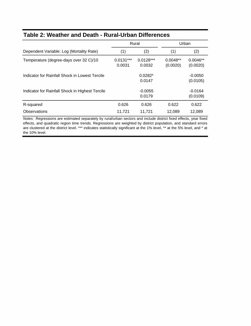
Dependent Variable: Log (Mortality Rate) (1) (2) (1) (2)

Temperature (degree-days over 32 C)/10 0.0131*** 0.0128*** 0.0048** 0.0046**0.0031 0.0032 (0.0020) (0.0020)

Indicator for Rainfall Shock in Lowest Tercile 0.0282* -0.00500.0147 (0.0105)

Indicator for Rainfall Shock in Highest Tercile -0.0055 -0.01640.0179 (0.0109)

R-squared 0.626 0.626 0.622 0.622

Observations 11,721 11,721 12,089 12,089

Rural Urban

Notes: Regressions are estimated separately by rural/urban sectors and include district fixed effects, year fixedeffects, and quadratic region time trends. Regressions are weighted by district population, and standard errorsare clustered at the district level. *** indicates statistically significant at the 1% level, ** at the 5% level, and * atthe 10% level.

Table 2: Weather and Death - Rural-Urban Differences

(1) (2) (3) (4) (5) (6) (7) (8)

Temperature (degree-days 0.0128*** 0.0133*** 0.0135*** 0.0046** 0.0045** 0.0044**over 32 C)/10 (0.0032) (0.0032) (0.0031) (0.0020) (0.0020) (0.0020)

Temperature (degree-days 0.0111*** 0.0024over 30 C)/10 (0.0032) (0.0014)

Temperature (degree-days 0.0017 -0.0014under 16 C)/10 (0.0025) (0.0015)

Temperature-rainfallinteractions included?

R-squared 0.626 0.628 0.626 0.626 0.622 0.623 0.621 0.622

Observations 11,721 11,721 11,721 11,721 12,089 12,089 12,089 12,089

Table 3: Weather and Death - Robustness

Notes: Regressions are estimated separately by rural/urban sectors and include district fixed effects, year fixed effects, and quadratic region time trends. Allregressions control for rainfall (upper/lower tercile dummies) as in Table 2. Regressions in columns (2) and (6) control for the interaction betweentemperature (degree-days over 32 C) and each rainfall tercile dummy variable. Regressions are weighted by district population, and standard errors areclustered at the district level. *** indicates statistically significant at the 1% level, ** at the 5% level, and * at the 10% level.

Urban

No Yes No No Yes No

Dependent Variable: Log(Mortality Rate)

Rural

No No

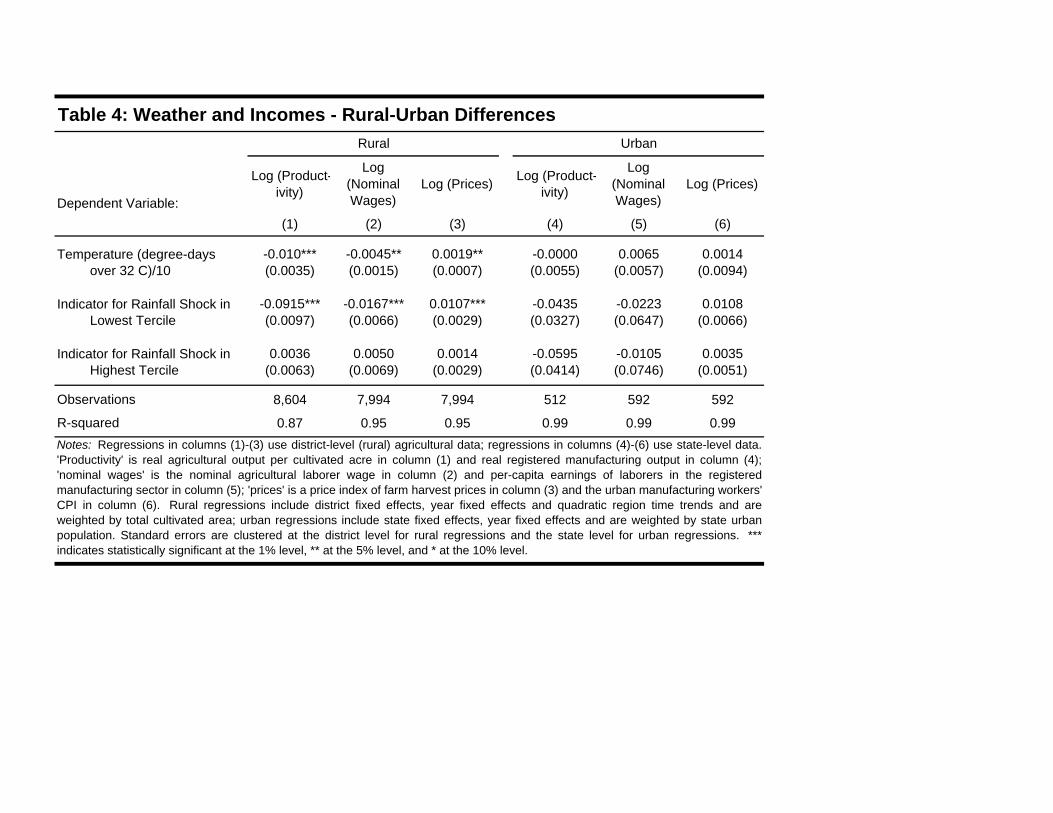
Table 4: Weather and Incomes - Rural-Urban Differences

Dependent Variable:

Log (Product-ivity)

Log (Nominal Wages)

Log (Prices)Log (Product-

ivity)

Log (Nominal Wages)

Log (Prices)

(1) (2) (3) (4) (5) (6)

Temperature (degree-days -0.010*** -0.0045** 0.0019** -0.0000 0.0065 0.0014over 32 C)/10 (0.0035) (0.0015) (0.0007) (0.0055) (0.0057) (0.0094)

Indicator for Rainfall Shock in -0.0915*** -0.0167*** 0.0107*** -0.0435 -0.0223 0.0108Lowest Tercile (0.0097) (0.0066) (0.0029) (0.0327) (0.0647) (0.0066)

Indicator for Rainfall Shock in 0.0036 0.0050 0.0014 -0.0595 -0.0105 0.0035Highest Tercile (0.0063) (0.0069) (0.0029) (0.0414) (0.0746) (0.0051)

Observations 8,604 7,994 7,994 512 592 592

R-squared 0.87 0.95 0.95 0.99 0.99 0.99

Notes: Regressions in columns (1)-(3) use district-level (rural) agricultural data; regressions in columns (4)-(6) use state-level data.'Productivity' is real agricultural output per cultivated acre in column (1) and real registered manufacturing output in column (4);'nominal wages' is the nominal agricultural laborer wage in column (2) and per-capita earnings of laborers in the registeredmanufacturing sector in column (5); 'prices' is a price index of farm harvest prices in column (3) and the urban manufacturing workers'CPI in column (6). Rural regressions include district fixed effects, year fixed effects and quadratic region time trends and areweighted by total cultivated area; urban regressions include state fixed effects, year fixed effects and are weighted by state urbanpopulation. Standard errors are clustered at the district level for rural regressions and the state level for urban regressions. ***indicates statistically significant at the 1% level, ** at the 5% level, and * at the 10% level.

Rural Urban

< 16 C 16C - 32 C >32 C

(1) (2) (3) (4) (5)

A. Based on Hadley 3, A1F1Pooled -0.010 -0.139 0.659 0.510 0.462

(0.030) (0.045) (0.126) (0.125) (0.142)

Rural Areas -0.030 -0.164 0.853 0.658 0.617(0.039) (0.055) (0.153) (0.126) (0.173)

Urban Areas 0.036 0.013 0.090 0.112 0.116(0.033) (0.058) (0.105) (0.101) (0.116)

B. Based on CCSM3, A2Pooled -0.010 0.039 0.145 0.176 0.116

(0.013) (0.042) (0.028) (0.061) (0.084)

Rural Areas -0.015 0.071 0.189 0.245 0.207(0.016) (0.049) (0.035) (0.074) (0.099)

Urban Areas 0.009 0.016 0.028 0.052 -0.078(0.013) (0.042) (0.022) (0.054) (0.092)

Impact of Change in Days with TemperatureTotal

Temperature Impact =

(1)+(2)+(3)

Temperature and

Precipitation Impact

Table 5: Climate Change and Mortality - Forecasted Percentage Impacts in 2070-2099, by Region

Notes : Forecasted percentage impacts of climate change scenarios in two leading climatological ('global circulation')models, separately by urban/rural/pooled regions. Reported numbers correspond to elements of equation (6), averagedover all districts (weighted by average population between 1957 and 2000). Estimates are based on regression models thatcontrol for unrestricted year effects, region-specific quadratic polynomials in time, and unrestricted district-area effects, anduse coefficient estimates that are weighted by census population. Projections compare historical period averagetemperatures (averaged over 1957-2000) with those predicted to occur by the end of the century (averaged over 2070-2099) in each given climatological model. Standard deviations are based on regression standard errors that are clusteredby district. See text for more details.

< 16 C 16C - 32 C >32 C

(1) (2) (3) (4) (5)

A. Based on Hadley 3, A1F12010-2039 -0.009 0.027 0.057 0.075 0.037

(0.014) (0.026) (0.012) (0.039) (0.054)

2040-2069 -0.011 -0.013 0.270 0.246 0.205(0.025) (0.028) (0.050) (0.069) (0.086)

2070-2099 -0.010 -0.139 0.659 0.510 0.462(0.030) (0.045) (0.126) (0.125) (0.142)

B. Based on CCSM3, A22010-2039 -0.006 0.082 -0.073 0.003 -0.054

(0.010) (0.016) (0.015) (0.018) (0.041)

2040-2069 -0.008 0.097 0.002 0.091 0.031(0.006) (0.023) (0.005) (0.023) (0.050)

2070-2099 -0.008 0.039 0.145 0.176 0.116(0.013) (0.042) (0.028) (0.061) (0.084)

Table 6: Climate Change and Mortality - Forecasted Percentage Impacts, by Time Horizon

Impact of Change in Days with Temperature

Total Temperature

Impact = (1)+(2)+(3)

Temperature and

Precipitation Impact

Notes : Forecasted percentage impacts of climate change scenarios in two leading climatological ('globalcirculation') models, averaged over all of India (weighted by population), separately for each of three time horizons.Reported numbers correspond to elements of equation (6), averaged over all districts (weighted by averagepopulation between 1957 and 2000). Estimates are based on regression models that control for unrestricted yeareffects, region-specific quadratic polynomials in time, and unrestricted district-area effects, and use coefficientestimates that are weighted by census population. Projections compare historical period average temperatures(averaged over 1957-2000) with those predicted to occur over the average within each of three time horizons.Standard deviations are based on regression standard errors that are clustered by district. See text for moredetails.