National Park Service U.S. Department of the Interior Natural Resource Program Center Fort Collins, Colorado

Weather and Climate Inventory National Park Service Southeast Coast Network

Natural Resource Technical Report NPS/SECN/NRTR—2007/010

ON THE COVER Cape Lookout National Seashore Photograph copyrighted by National Park Service

Weather and Climate Inventory National Park Service Southeast Coast Network Natural Resource Technical Report NPS/SECN/NRTR—2007/010 WRCC Report 2007-06 Christopher A. Davey, Kelly T. Redmond, and David B. Simeral Western Regional Climate Center Desert Research Institute 2215 Raggio Parkway Reno, Nevada 89512-1095 April 2007 U.S. Department of the Interior National Park Service Natural Resource Program Center Fort Collins, Colorado

ii

The Natural Resource Publication series addresses natural resource topics that are of interest and applicability to a broad readership in the National Park Service and to others in the management of natural resources, including the scientific community, the public, and the National Park Service conservation and environmental constituencies. Manuscripts are peer-reviewed to ensure that the information is scientifically credible, technically accurate, appropriately written for the intended audience, and designed and published in a professional manner. The Natural Resources Technical Reports series is used to disseminate the peer-reviewed results of scientific studies in the physical, biological, and social sciences for both the advancement of science and the achievement of the National Park Service mission. The reports provide contributors with a forum for displaying comprehensive data that are often deleted from journals because of page limitations. Current examples of such reports include the results of research that address natural resource management issues; natural resource inventory and monitoring activities; resource assessment reports; scientific literature reviews; and peer-reviewed proceedings of technical workshops, conferences, or symposia. Views and conclusions in this report are those of the authors and do not necessarily reflect policies of the National Park Service. Mention of trade names or commercial products does not constitute endorsement or recommendation for use by the National Park Service. Printed copies of reports in these series may be produced in a limited quantity and they are only available as long as the supply lasts. This report is also available from the Natural Resource Publications Management website (http://www.nature.nps.gov/publications/NRPM) on the Internet or by sending a request to the address on the back cover. Please cite this publication as follows: Davey, C. A., K. T. Redmond, and D. B. Simeral. 2007. Weather and Climate Inventory, National Park Service, Southeast Coast Network. Natural Resource Technical Report NPS/SECN/NRTR—2007/010. National Park Service, Fort Collins, Colorado. NPS/SECN/NRTR—2007/010, April 2007

iii

Contents Page

Figures ............................................................................................................................................ v Tables ........................................................................................................................................... vi Appendixes ................................................................................................................................. vii Acronyms ................................................................................................................................... viii Executive Summary ....................................................................................................................... x Acknowledgements ..................................................................................................................... xii 1.0. Introduction ............................................................................................................................. 1 1.1. Network Terminology ...................................................................................................... 2 1.2. Weather versus Climate Definitions ................................................................................ 4 1.3. Purpose of Measurements ................................................................................................ 4 1.4. Design of Climate-Monitoring Programs ........................................................................ 5 2.0. Climate Background .............................................................................................................. 10 2.1. Climate and the SECN Environment ............................................................................. 10 2.2. Spatial Variability .......................................................................................................... 11 2.3. Temporal Variability ...................................................................................................... 17 2.4. Parameter Regression on Independent Slopes Model .................................................... 17 3.0. Methods ................................................................................................................................. 20 3.1. Metadata Retrieval ......................................................................................................... 20 3.2. Criteria for Locating Stations ......................................................................................... 22 4.0. Station Inventory ................................................................................................................... 23 4.1. Climate and Weather Networks ..................................................................................... 23 4.2. Station Locations ........................................................................................................... 25

iv

Contents (continued) Page

5.0. Conclusions and Recommendations ..................................................................................... 51 5.1. Southeast Coast Inventory and Monitoring Network .................................................... 51 5.2. Spatial Variations in Mean Climate ............................................................................... 51 5.3. Climate Change Detection ............................................................................................. 52 5.4. Aesthetics ....................................................................................................................... 52 5.5. Information Access ........................................................................................................ 52 5.6. Summarized Conclusions and Recommendations ......................................................... 53 6.0. Literature Cited ..................................................................................................................... 54

v

Figures Page

Figure 1.1. Map of the Southeast Coast Network ........................................................................ 3 Figure 2.1. Mean annual precipitation, 1961–1990, for the SECN ............................................ 12 Figure 2.2. Mean monthly precipitation at selected locations in the SECN .............................. 13 Figure 2.3. Mean annual temperature, 1961–1990, for the SECN ............................................. 14 Figure 2.4. Mean January minimum temperature, 1961–1990, for the SECN ........................... 15 Figure 2.5. Mean July maximum temperature, 1961–1990, for the SECN ................................ 16 Figure 2.6. Precipitation time series, 1895-2005, for selected regions

in the SECN ............................................................................................................. 18 Figure 2.7. Temperature time series, 1895-2005, for selected regions

in the SECN ............................................................................................................. 19 Figure 4.1. Station locations for the SECN park units in North Carolina .................................. 31 Figure 4.2. Station locations for the SECN park units along the Florida

and Georgia coasts ................................................................................................... 37 Figure 4.3. Station locations for the SECN park units in Alabama,

Georgia, and South Carolina .................................................................................... 47

vi

Tables Page

Table 1.1. Park units in the Southeast Coast Network .................................................................. 2 Table 3.1. Primary metadata fields for SECN weather/climate stations ..................................... 21 Table 4.1. Weather/climate networks represented within the SECN .......................................... 23 Table 4.2. Number of stations within or nearby SECN park units ............................................. 26 Table 4.3. Weather/climate stations for the SECN park units in

North Carolina ........................................................................................................... 28 Table 4.4. Weather/climate stations for the SECN park units along the

Florida and Georgia coasts ......................................................................................... 33 Table 4.5. Weather/climate stations for the SECN park units in

Alabama, Georgia, and South Carolina ..................................................................... 40

vii

Appendixes Page

Appendix A. Glossary ............................................................................................................... 58 Appendix B. Climate-monitoring principles ............................................................................. 60 Appendix C. Factors in operating a climate network ................................................................ 63 Appendix D. General design considerations for weather/climate-monitoring programs .......... 65 Appendix E. Master metadata field list ..................................................................................... 85 Appendix F. Electronic supplements ........................................................................................ 87 Appendix G. Descriptions of weather/climate-monitoring networks ........................................ 88

viii

Acronyms AASC American Association of State Climatologists ACIS Applied Climate Information System ASOS Automated Surface Observing System AWOS Automated Weather Observing System BLM Bureau of Land Management CAHA Cape Hatteras National Seashore CALO Cape Lookout National Seashore CANA Canaveral National Seashore CASA Castillo de San Marcos National Monument CASTNet Clean Air Status and Trends Network CHAT Chattahoochee River National Recreation Area CHPI Charles Pinckney National Historic Site CONG Congaree National Park COOP Cooperative Observer Program CRN NOAA Climate Reference Network CUIS Cumberland Island National Seashore CWOP Citizen Weather Observer Program DFIR Double-Fence Intercomparison Reference DST daylight savings time ENSO El Niño Southern Oscillation EPA Environmental Protection Agency FAA Federal Aviation Administration FAWN Florida Automated Weather Network FOCA Fort Caroline National Memorial FOFR Fort Frederica National Monument FOMA Fort Mantanzas National Monument FOPU Fort Pulaski National Monument FORA Fort Raleigh National Historic Site FOSU Fort Sumter National Monument FIPS Federal Information Processing Standards GMT Greenwich Mean Time GOES Geostationary Operational Environmental Satellite GPMP Gaseous Pollutant Monitoring Program GPS Global Positioning System GPS-MET NOAA ground-based GPS meteorology HOBE Horseshoe Bend National Military Park I&M NPS Inventory and Monitoring Program KEMO Kennesaw Mountain National Battlefield Park LEO Low Earth Orbit LST local standard time MDN Mercury Deposition Network MOCR Moores Creek National Battlefield NADP National Atmospheric Deposition Program NASA National Aeronautics and Space Administration

ix

NCDC National Climatic Data Center NetCDF Network Common Data Form NOAA National Oceanic and Atmospheric Administration NPS National Park Service NRCS Natural Resources Conservation Service NWS National Weather Service OCMU Ocmulgee National Monument PRISM Parameter Regression on Independent Slopes Model RAWS Remote Automated Weather Station network RCC regional climate center SAO Surface Airways Observation network SECN Southeast Coast Inventory and Monitoring Network SNOTEL Snowfall Telemetry network SOD Summary Of the Day Surfrad Surface Radiation Budget network TIMU Timucuan Ecological and Historic Preserve USDA U.S. Department of Agriculture USGS U.S. Geological Survey UTC Coordinated Universal Time WBAN Weather Bureau Army Navy WMO World Meteorological Organization WRBR Wright Brothers National Memorial WRCC Western Regional Climate Center WX4U Weather For You network

x

Executive Summary Climate is a dominant factor driving the physical and ecologic processes affecting the Southeast Coast Inventory and Monitoring Network (SECN). Climate variations are responsible for short- and long-term changes in ecosystem fluxes of energy and matter and have profound effects on underlying geomorphic and biogeochemical processes. Southeastern climates are humid and warm-temperate to subtropical, with significant maritime influences from the Atlantic Ocean and Gulf of Mexico. The southern end of the Appalachian Mountains also influences climate patterns in the SECN park units located in eastern Alabama and northern Georgia. Extreme weather events in the SECN drive both coastal and riverine geomorphic changes. Impacts from storm washover episodes associated with strong nor’easter events in the winter and tropical systems in the summer and fall, and the recovery periods from such events, are an important issue for coastal SECN ecosystems. Thunderstorms are an integral part of the SECN climate, especially during the spring and summer months. The El Niño Southern Oscillation (ENSO) plays a large role in the interannual variations of the climate of the SECN, with El Niño years typically bringing lower temperatures in winter and spring, increased winter precipitation, and fewer tropical systems. Potential sea-level rises due to predicted global-scale climate changes are also a concern for many SECN park units. Periods of prolonged drought introduce stressors to vegetation communities with potentially severe effects. Human impacts on the landscape of the SECN region have introduced local- and regional-scale climate changes in the SECN, many of which are adversely impacting the region’s plant and animal communities. Because of its influence on the ecology of SECN park units and the surrounding areas, climate was identified as a high-priority vital sign for SECN and is one of the 12 basic inventories to be completed for all National Park Service (NPS) Inventory and Monitoring Program (I&M) networks. This project was initiated to inventory past and present climate monitoring efforts. In this report, we provide the following information:

• Overview of broad-scale climatic factors and zones important to SECN park units. • Inventory of weather and climate station locations in and near SECN park units relevant to

the NPS I&M Program. • Results of an inventory of metadata on each weather station, including affiliations for

weather-monitoring networks, types of measurements recorded at these stations, and information about the actual measurements (length of record, etc.).

• Initial evaluation of the adequacy of coverage for existing weather stations and recommendations for improvements in monitoring weather and climate.

Mean annual precipitation in the SECN is fairly uniform but increases gradually towards the Atlantic coast and also towards western portions of SECN. Some of the wettest park units in the SECN receive over 1400 millimeters (mm) of precipitation every year. The driest park units in the SECN generally receive between 1000 and 1200 mm of precipitation each year. Western portions of the SECN tend to receive more of their annual precipitation in winter, while park units along the Atlantic coast tend to get more precipitation during the summer months. Temperatures in the SECN vary largely as a function of latitude and proximity to the coast. Mean annual temperatures are coolest for the park units in northern Georgia (about 14°C) while some SECN park units in Florida see mean annual temperatures above 20°C. Winter

xi

temperatures are fairly mild, showing a strong latitudinal gradient. During the summer months, factors such as elevation and proximity to the coast become more important. Summer temperatures are moderated along the coastal SECN park units, while park units immediately inland of the coast are generally a few degrees warmer. Although the proximity of oceans generally moderates extreme temperature conditions, with average summertime maximum temperatures around 30°C, daytime temperatures can occasionally reach 40°C. Precipitation and temperature trends are generally neutral throughout the SECN. Large variations in temperature patterns for the SECN over the past century highlight the emphasis on measurement consistency that is needed in order to properly detect long-term climatic changes. Through a search of national databases and inquiries to NPS staff, we have identified 15 weather and climate stations within SECN park units. The most stations are found in Cape Hatteras National Seashore (CAHA) and Congaree National Park (CONG). Both park units have four weather/climate stations. The SECN office was helpful in identifying weather/climate stations within SECN park units. Many SECN park units, historical sites or other memorials in particular, have no weather/climate stations at or within park boundaries. As a result, these park units must rely heavily on stations outside of the park units for their weather and climate data. Fortunately, each of these park units have numerous near-real-time and long-term weather/climate stations nearby. For those park units that do have weather/climate stations inside their boundaries, very few of these stations have verifiable long-term data records. Those records which are available are valuable for climate monitoring efforts in the SECN, highlighting the importance of retaining such long-term sites. The national seashore park units in the SECN, CAHA and Cape Lookout National Seashore (CALO) in particular, contain large stretches of barrier islands that currently have no weather/climate station coverage. The stations that are available are located at the edges of these barrier islands or are usually a significant distance away from the barrier islands, either at inland sites or on ocean buoys. New station installations on previously-unsampled stretches of barrier islands would be helpful for monitoring coast-interior climate gradients and other climate dynamics that work to shape the coastal ecosystems of the SECN.

xii

Acknowledgements This work was supported and completed under Task Agreement H8R07010001, with the Great Basin Cooperative Ecosystem Studies Unit. We would like to acknowledge very helpful assistance from various National Park Service personnel associated with the Southeast Coast Inventory and Monitoring Network. Particular thanks are extended to Christina Wright and Joe DeVivo. We also thank John Gross, Margaret Beer, Grant Kelly, Greg McCurdy, and Heather Angeloff for all their help. Seth Gutman with the National Oceanic and Atmospheric Administration Earth Systems Research Laboratory provided valuable input on the GPS-MET station network. Portions of the work were supported by the NOAA Western Regional Climate Center.

1

1.0. Introduction Weather and climate are key drivers in ecosystem structure and function. Global- and regional-scale climate variations will have a tremendous impact on natural systems (Chapin et al. 1996; Schlesinger 1997; Jacobson et al. 2000; Bonan 2002). Long-term patterns in temperature and precipitation provide first-order constraints on potential ecosystem structure and function. Secondary constraints are realized from the intensity and duration of individual weather events and, additionally, from seasonality and inter-annual climate variability. These constraints influence the fundamental properties of ecologic systems, such as soil–water relationships, plant–soil processes, and nutrient cycling, as well as disturbance rates and intensity. These properties, in turn, influence the life-history strategies supported by a climatic regime (Neilson 1987; DeVivo et al. 2005). Given the importance of climate, it is one of 12 basic inventories to be completed by the National Park Service (NPS) Inventory and Monitoring Program (I&M) network (I&M 2006). As primary environmental drivers for the other vital signs, weather and climate patterns present various practical and management consequences and implications for the NPS (Oakley et al. 2003). Most park units observe weather and climate elements as part of their overall mission. The lands under NPS stewardship provide many excellent locations for monitoring climatic conditions. It is essential that park units within the Southeast Coast Inventory and Monitoring Network (SECN) have an effective climate-monitoring system in place to track climate changes and to aid in management decisions relating to these changes. The purpose of this report is to determine the current status of weather and climate monitoring within the SECN (Table 1.1; Figure 1.1). In this report, we provide the following informational elements:

• Overview of broad-scale climatic factors and zones important to SECN park units. • Inventory of locations for all weather stations in and near SECN park units that are relevant

to the NPS I&M networks. • Results of metadata inventory for each station, including weather-monitoring network

affiliations, types of recorded measurements, and information about actual measurements (length of record, etc.).

• Initial evaluation of the adequacy of coverage for existing weather stations and recommendations for improvements in monitoring weather and climate.

The primary objectives for climate- and weather-monitoring in the SECN are as follows (DeVivo et al. 2005):

A. Determine status and trends in temperature and precipitation. B. Determine the severity and frequency of droughts. C. Determine the frequency of hurricanes, tropical storms, and other high-energy storm

events. D. Determine the frequency and distribution of lightning strikes. E. Determine status and trends in mean sea level.

2

1.1. Network Terminology Before proceeding, it is important to stress that this report discusses the idea of “networks” in two different ways. Modifiers are used to distinguish between NPS I&M networks and weather/climate station networks. See Appendix A for a full definition of these terms. 1.1.1. Weather/Climate Station Networks Most weather and climate measurements are made not from isolated stations but from stations that are part of a network operated in support of a particular mission. The limiting case is a network of one station, where measurements are made by an interested observer or group. Larger networks usually have additional inventory data and station-tracking procedures. Some national weather/climate networks are associated with the National Oceanic and Atmospheric Administration (NOAA), including the National Weather Service (NWS) Cooperative Observer Program (COOP). Other national networks include the interagency Remote Automated Weather Station network (RAWS) and the U.S. Department of Agriculture/Natural Resources Conservation Service (USDA/NRCS) Snowfall Telemetry (SNOTEL) and snowcourse networks. Usually a single agency, but sometimes a consortium of interested parties, will jointly support a particular weather/climate network. Table 1.1. Park units in the Southeast Coast Network.

Acronym Name CAHA Cape Hatteras National Seashore CALO Cape Lookout National Seashore CANA Canaveral National Seashore CASA Castillo de San Marcos National Monument CHAT Chattahoochee River National Recreation Area CHPI Charles Pinckney National Historic Site CONG Congaree National Park CUIS Cumberland Island National Seashore FOCA Fort Caroline National Memorial FOFR Fort Frederica National Monument FOMA Fort Mantanzas National Monument FOPU Fort Pulaski National Monument FORA Fort Raleigh National Historic Site FOSU Fort Sumter National Monument HOBE Horseshoe Bend National Military Park KEMO Kennesaw Mountain National Battlefield Park MOCR Moores Creek National Battlefield OCMU Ocmulgee National Monument TIMU Timucuan Ecological and Historic Preserve WRBR Wright Brothers National Memorial

3

Figure 1.1. Map of the Southeast Coast Network.

4

1.1.2. NPS I&M Networks Within the NPS, the system for monitoring various attributes in the participating park units (about 270–280 in total) is divided into 32 NPS I&M networks. These networks are collections of park units grouped together around a common theme, typically geographical. 1.2. Weather versus Climate Definitions It is also important to distinguish whether the primary use of a given station is for weather purposes or for climate purposes. Weather station networks are intended for near-real-time usage, where the precise circumstances of a set of measurements are typically less important. In these cases, changes in exposure or other attributes over time are not as critical. Climate networks, however, are intended for long-term tracking of atmospheric conditions. Siting and exposure are critical factors for climate networks, and it is vitally important that the observational circumstances remain essentially unchanged over the duration of the station record. Some climate networks can be considered hybrids of weather/climate networks. These hybrid climate networks can supply information on a short-term “weather” time scale and a longer-term “climate” time scale. In this report, “weather” generally refers to current (or near-real-time) atmospheric conditions, while “climate” is defined as the complete ensemble of statistical descriptors for temporal and spatial properties of atmospheric behavior (see Appendix A). Climate and weather phenomena shade gradually into each other and are ultimately inseparable. 1.3. Purpose of Measurements Climate inventory and monitoring climate activities should be based on a set of guiding fundamental principles. Any evaluation of weather/climate monitoring programs begins with asking the following question:

• What is the purpose of weather and climate measurements? Evaluation of past, present, or planned weather/climate monitoring activities must be based on the answer to this question. Weather and climate data and information constitute a prominent and widely requested component of the NPS I&M networks (I&M 2006). Within the context of the NPS, the following services constitute the main purposes for recording weather and climate observations:

• Provide measurements for real-time operational needs and early warnings of potential hazards (landslides, mudflows, washouts, fallen trees, plowing activities, fire conditions, aircraft and watercraft conditions, road conditions, rescue conditions, fog, restoration and remediation activities, etc.).

• Provide visitor education and aid interpretation of expected and actual conditions for visitors while they are in the park and for deciding if and when to visit the park.

• Establish engineering and design criteria for structures, roads, culverts, etc., for human comfort, safety, and economic needs.

5

• Consistently monitor climate over the long-term to detect changes in environmental drivers affecting ecosystems, including both gradual and sudden events.

• Provide retrospective data to understand a posteriori changes in flora and fauna. • Document for posterity the physical conditions in and near the park units, including mean,

extreme, and variable measurements (in time and space) for all applications. The last three items in the preceding list are pertinent primarily to the NPS I&M networks; however, all items are important to NPS operations and management. Most of the needs in this list overlap heavily. It is often impractical to operate separate climate measuring systems that also cannot be used to meet ordinary weather needs, where there is greater emphasis on timeliness and reliability. 1.4. Design of Climate-Monitoring Programs Determining the purposes for collecting measurements in a given weather/climate monitoring program will guide the process of identifying weather/climate stations suitable for the monitoring program. The context for making these decisions is provided in Chapter 2 where background on the SECN climate is presented. However, this process is only one step in evaluating and designing a climate-monitoring program. This process includes the following additional steps:

• Define park and network-specific monitoring needs and objectives. • Identify locations and data repositories of existing and historic stations. • Acquire existing data when necessary or practical. • Evaluate the quality of existing data. • Evaluate the adequacy of coverage of existing stations. • Develop a protocol for monitoring the weather and climate, including the following:

o Standardized summaries and reports of weather/climate data. o Data management (quality assurance and quality control, archiving, data access, etc.).

• Develop and implement a plan for installing or modifying stations, as necessary. Throughout the design process, there are various factors that require consideration in evaluating weather and climate measurements. Many of these factors have been summarized by Dr. Tom Karl, director of the NOAA National Climatic Data Center (NCDC), and widely distributed as the “Ten Principles for Climate Monitoring” (Karl et al. 1996a; NRC 2001). These principals are presented in Appendix B, and the guidelines are embodied in many of the comments made throughout this report. The most critical factors are presented here. In addition, an overview of requirements necessary to operate a climate network is provided in Appendix C, with further discussion in Appendix D. 1.4.1. Need for Consistency A principal goal in climate monitoring is to detect and characterize slow and sudden changes in climate through time. This is of less concern for day-to-day weather changes, but it is of paramount importance for climate variability and change. There are many ways whereby changes in techniques for making measurements, changes in instruments or their exposures, or seemingly innocuous changes in site characteristics can lead to apparent changes in climate. Safeguards must be in place to avoid these false sources of temporal “climate” variability if we are to draw correct inferences about climate behavior over time from archived measurements.

6

For climate monitoring, consistency through time is vital, counting at least as important as absolute accuracy. Sensors record only what is occurring at the sensor—this is all they can detect. It is the responsibility of station or station network managers to ensure that observations are representative of the spatial and temporal climate scales that we wish to record. 1.4.2. Metadata Changes in instruments, site characteristics, and observing methodologies can lead to apparent changes in climate through time. It is therefore vital to document all factors that can bear on the interpretation of climate measurements and to update the information repeatedly through time. This information (“metadata,” data about data) has its own history and set of quality-control issues that parallel those of the actual data. There is no single standard for the content of climate metadata, but a simple rule suffices:

• Observers should record all information that could be needed in the future to interpret observations correctly without benefit of the observers’ personal recollections.

Such documentation includes notes, drawings, site forms, and photos, which can be of inestimable value if taken in the correct manner. That stated, it is not always clear to the metadata provider what is important for posterity and what will be important in the future. It is almost impossible to “over document” a station. Station documentation is greatly underappreciated and is seldom thorough enough (especially for climate purposes). Insufficient attention to this issue often lowers the present and especially future value of otherwise useful data. The convention followed throughout climatology is to refer to metadata as information about the measurement process, station circumstances, and data. The term “data” is reserved solely for the actual weather and climate records obtained from sensors. 1.4.3. Maintenance Inattention to maintenance is the greatest source of failure in weather/climate stations and networks. Problems begin to occur soon after sites are deployed. A regular visit schedule must be implemented, where sites, settings (e.g., vegetation), sensors, communications, and data flow are checked routinely (once or twice a year at a minimum) and updated as necessary. Parts must be changed out for periodic recalibration or replacement. With adequate maintenance, the entire instrument suite should be replaced or completely refurbished about once every five to seven years. Simple preventative maintenance is effective but requires much planning and skilled technical staff. Changes in technology and products require retraining and continual re-education. Travel, logistics, scheduling, and seasonal access restrictions consume major amounts of time and budget but are absolutely necessary. Without such attention, data gradually become less credible and then often are misused or not used at all. 1.4.4. Automated versus Manual Stations Historic stations often have depended on manual observations and many continue to operate in this mode. Manual observations frequently produce excellent data sets. Sensors and data are

7

simple and intuitive, well tested, and relatively cheap. Manual stations have much to offer in certain circumstances and can be a source of both primary and backup data. However, methodical consistency for manual measurements is a constant challenge, especially with a mobile work force. Operating manual stations takes time and needs to be done on a regular schedule, though sometimes the routine is welcome. Nearly all newer stations are automated. Automated stations provide better time resolution, increased (though imperfect) reliability, greater capacity for data storage, and improved accessibility to large amounts of data. The purchase cost for automated stations is higher than for manual stations. A common expectation and serious misconception is that an automated station can be deployed and left to operate on its own. In reality, automation does not eliminate the need for people but rather changes the type of person that is needed. Skilled technical personnel are needed and must be readily available, especially if live communications exist and data gaps are not wanted. Site visits are needed at least annually and spare parts must be maintained. Typical annual costs for sensors and maintenance at the major national networks are $1500–2500 per station per year but these costs still can vary greatly depending on the kind of automated site. 1.4.5. Communications With manual stations, the observer is responsible for recording and transmitting station data. Data from automated stations, however, can be transmitted quickly for access by research and operations personnel, which is a highly preferable situation. A comparison of communication systems for automated and manual stations shows that automated stations generally require additional equipment, more power, higher transmission costs, attention to sources of disruption or garbling, and backup procedures (e.g. manual downloads from data loggers). Automated stations are capable of functioning normally without communication and retaining many months of data. At such sites, however, alerts about station problems are not possible, large gaps can accrue when accessible stations quit, and the constituencies needed to support such stations are smaller and less vocal. Two-way communications permit full recovery from disruptions, ability to reprogram data loggers remotely, and better opportunities for diagnostics and troubleshooting. In virtually all cases, two-way communications are much preferred to all other communication methods. However, two-way communications require considerations of cost, signal access, transmission rates, interference, and methods for keeping sensor and communication power loops separate. Two-way communications are frequently impossible (no service) or impractical, expensive, or power consumptive. Two-way methods (cellular, land line, radio, Internet) require smaller up-front costs as compared to other methods of communication and have variable recurrent costs, starting at zero. Satellite links work everywhere (except when blocked by trees or cliffs) and are quite reliable but are one-way and relatively slow, allow no re-transmissions, and require high up-front costs ($3000–4000) but no recurrent costs. Communications technology is changing constantly and requires vigilant attention by maintenance personnel. 1.4.6. Quality Assurance and Quality Control Quality control and quality assurance are issues at every step through the entire sequence of sensing, communication, storage, retrieval, and display of environmental data. Quality assurance is an umbrella concept that covers all data collection and processing (start-to-finish) and ensures

8

that credible information is available to the end user. Quality control has a more limited scope and is defined by the International Standards Organization as “the operational techniques and activities that are used to satisfy quality requirements.” The central problem can be better appreciated if we approach quality control in the following way.

• Quality control is the evaluation, assessment, and rehabilitation of imperfect data by utilizing other imperfect data.

The quality of the data only decreases with time once the observation is made. The best and most effective quality control, therefore, consists in making high-quality measurements from the start and then successfully transmitting the measurements to an ingest process and storage site. Once the data are received from a monitoring station, a series of checks with increasing complexity can be applied, ranging from single-element checks (self-consistency) to multiple-element checks (inter-sensor consistency) to multiple-station/single-element checks (inter-station consistency). Suitable ancillary data (battery voltages, data ranges for all measurements, etc.) can prove extremely useful in diagnosing problems. There is rarely a single technique in quality control procedures that will work satisfactorily for all situations. Quality-control procedures must be tailored to individual station circumstances, data access and storage methods, and climate regimes. The fundamental issue in quality control centers on the tradeoff between falsely rejecting good data (Type I error) and falsely accepting bad data (Type II error). We cannot reduce the incidence of one type of error without increasing the incidence of the other type. In weather and climate data assessments, since good data are absolutely crucial for interpreting climate records properly, Type I errors are deemed far less desirable than Type II errors. Not all observations are equal in importance. Quality-control procedures are likely to have the greatest difficulty evaluating the most extreme observations, where independent information usually must be sought and incorporated. Quality-control procedures involving more than one station usually involve a great deal of infrastructure with its own (imperfect) error-detection methods, which must be in place before a single value can be evaluated. 1.4.7. Standards Although there is near-universal recognition of the value in systematic weather and climate measurements, these measurements will have little value unless they conform to accepted standards. There is not a single source for standards for collecting weather and climate data nor a single standard that meets all needs. Measurement standards have been developed by the American Association of State Climatologists (AASC 1985), U.S. Environmental Protection Agency (EPA 1987), World Meteorological Organization (WMO 1983; 2005), Finklin and Fischer (1990), National Wildfire Coordinating Group (2004), and the RAWS program (Bureau of Land Management [BLM] 1997). Variations to these measurement standards also have been offered by instrument makers (e.g., Tanner 1990).

9

1.4.8. Who Makes the Measurements? The lands under NPS stewardship provide many excellent locations to host the monitoring of climate by the NPS or other collaborators. These lands are largely protected from human development and other land changes that can impact observed climate records. Most park units historically have observed weather/climate elements as part of their overall mission. Many of these measurements come from station networks managed by other agencies, with observations taken or overseen by NPS personnel, in some cases, or by collaborators from the other agencies. National Park Service units that are small, lack sufficient resources, or lack sites presenting adequate exposure may benefit by utilizing weather/climate measurements collected from nearly stations.

10

2.0. Climate Background The ecosystems in the SECN, both aquatic and terrestrial, are strongly influenced by climate characteristics (DeVivo et al. 2005). Weather and climate drive freshwater inputs to aquatic and wetland systems. Climate is a key driver of fire frequency and magnitude in terrestrial systems. Extreme weather events in the SECN drive both coastal and riverine geomorphic changes. It is essential that the SECN park units have an effective climate monitoring system to track climate changes and to aid in management decisions relating to these changes. These efforts are needed in order to support current vital sign monitoring activities within the park units of the SECN. In order to do this, however, it is essential to understand the climate characteristics of the SECN, as discussed in this chapter. 2.1. Climate and the SECN Environment Southeastern climates are humid and warm-temperate to subtropical (Ruffner 1985; White et al. 1998). Major variation in climate occurs with change in latitude and elevation. Longitude has a more subtle influence on climate than latitude, as a result of maritime influence to the south and east and continental influences to the north and west. Latitudinal gradients in temperature are steeper in winter than in summer, producing a strong geographic pattern in freeze-free periods and cold temperatures (White et al. 1998). Precipitation throughout the network typically comes in the form of rain from winter and spring storm fronts, and tropical storms and hurricanes in the summer and/or early fall (White et al. 1998). The winter and spring storms that impact the SECN include coastal nor’easter storms that develop just off the southeastern U.S. coast before moving up the eastern seaboard. Thunderstorms are an integral part of the SECN climate, especially during the spring and summer months. In fact, northern Florida, including such park units as CANA, CASA, and FOMA, is one of the most active areas for lightning in the entire U.S. (Changnon 1988a; 1988b; Hodanish et al. 1997; Zajac and Rutledge 2001; Orville et al. 2001; DeVivo et al. 2005. The El Niño Southern Oscillation (ENSO) plays a large role in the interannual variations of the climate of the SECN. El Niño years typically bring lower temperatures in winter and spring and increased winter precipitation throughout the SECN. During La Niña years, however, drought conditions can occur and have significant negative consequences on SECN ecosystems (DeVivo et al. 2005). Further, ENSO has a strong influence on the number of Atlantic Basin tropical storms and hurricanes, which regularly impact portions of the SECN during the summer and fall months (Smith 1999; Lyons 2004). Hurricanes play a significant role in shaping the structure and characteristics of SECN ecosystems, particularly coastal systems. During La Niña events, the average number of hurricanes in the Atlantic Basin increases compared to El Niño years (Gray 1984a; Gray 1984b; Landsea 1993; Goldenberg and Shapiro 1996; Bove et al. 1998). Several of the management issues identified for the park units of the SECN (DeVivo et al. 2005) have impacts on local climate, and vice versa. Impacts from storm washover episodes associated with strong nor’easter events in the winter and tropical systems in the summer and fall, and the recovery periods from such events, are an important issue for barrier islands in many of the SECN park units along the Atlantic coast (Hosier and Cleary 1978). In addition, potential sea-

11

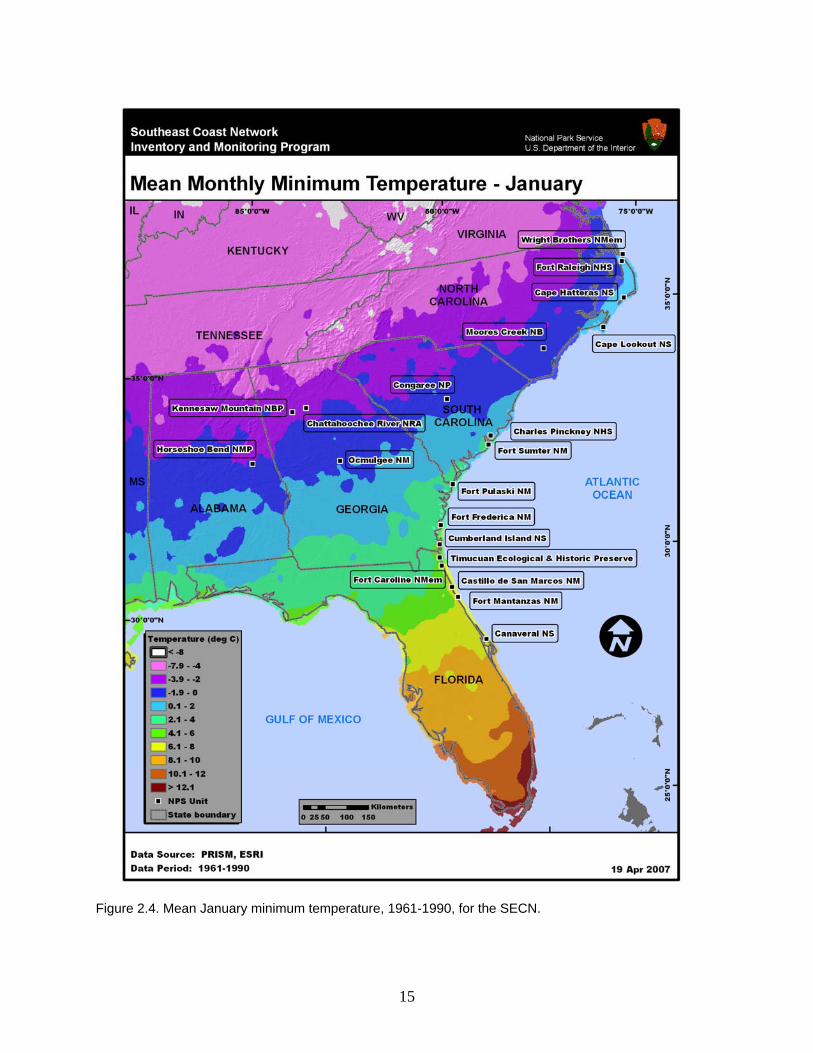
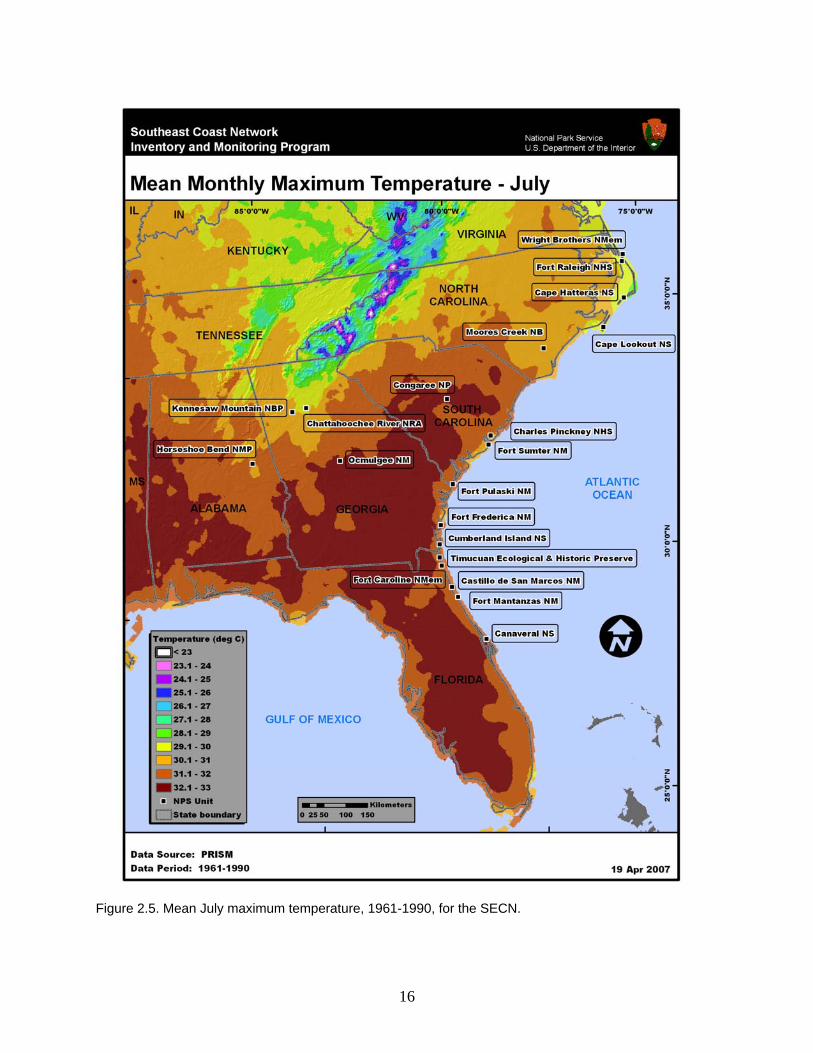
level rises due to predicted global-scale climate changes are also a concern along these coastal park units (Zimmerman et al. 1991; NAST 2001). Periods of prolonged drought introduce stressors to vegetation communities with potentially severe effects. For instance, wildfire and forest-pest (i.e., turpentine beetle) outbreaks at park units such as CONG have both been linked to periods of prolonged drought (DeVivo et al. 2005). Human impacts on the landscape of the SECN region have introduced disturbances and land-use heterogeneities that have introduced local- and regional-scale climate changes in the SECN, many of which are adversely impacting the region’s plant and animal communities. Exotic plant species introduced to the SECN have already had negative impacts on the region’s ecosystems. The spread of these non-native plant species could be accelerated in response to future climate changes, particularly in those areas where native plant species are unable to adapt to the climate changes (DeVivo et al. 2005). 2.2. Spatial Variability Much of the SECN lies on the Coastal Plain and Piedmont regions of the southeastern U.S. Therefore, both the Atlantic Ocean and the Gulf of Mexico are strong drivers of the climate characteristics of the SECN. The southern end of the Appalachian Mountains also influences climate patterns in the SECN park units located in eastern Alabama and northern Georgia. Mean annual precipitation in the SECN (Figure 2.1) is fairly uniform but increases gradually towards the Atlantic coast and also towards western portions of SECN. Some of the wettest park units in the SECN, including CALO and HOBE, see mean annual precipitation totals in excess of 1400 mm. The driest park units in the SECN, including CONG and OCMU, are located in the Piedmont region of Georgia and South Carolina. These locations generally receive between 1000 and 1200 mm of precipitation every year. During the course of a given year, western portions of the SECN tend to receive more of their annual precipitation during the winter months (Figure 2.2). However, for SECN park units along the Atlantic coast, precipitation tends to reach a maximum during the late summer months, with substantially drier conditions from fall through spring. Much of the summertime precipitation along the coast can be attributed to daily land-sea breeze interactions (Marshall et al. 2004) along with occasional tropical storm and hurricane activity (NAST 2001). Temperatures in the SECN vary largely as a function of latitude and proximity to the coast. Mean annual temperatures are coolest for the park units in northern Georgia, averaging around 14°C (Figure 2.3). The warmest park unit in the SECN is CANA, with a mean annual temperature above 20°C. The latitudinal gradient in temperatures is quite evident in winter temperatures (White et al. 1998). For example, January minimum temperatures (Figure 2.4) are warmest for CANA, at just under 8°C. The coldest SECN park units are in northern Georgia, where mean January minimum temperatures are just below -4°C. During the summer months, latitude becomes less of a driving factor for SECN temperatures and factors such as elevation and proximity to the coast become more important. Mean July maximum temperatures, for example, are moderated along the immediate coast in the SECN (Figure 2.5). Locations immediately inland of the coast are generally a few degrees warmer than coastal locations. Some of the coolest coastal park units are found along coastal North Carolina,

12

Figure 2.1. Mean annual precipitation, 1961-1990, for the SECN.

13

a)

b)

c)

Figure 2.2. Mean monthly precipitation at selected locations in the SECN. Atlanta Bolton (a) is near CHAT and KEMO, Cape Hatteras WSO (b; also known as Cape Hatteras Billy Mitchell Airport) is in CAHA, and Brunswick (c) is near CUIS and FOFR.

14

Figure 2.3. Mean annual temperature, 1961-1990, for the SECN.

15

Figure 2.4. Mean January minimum temperature, 1961-1990, for the SECN.

16

Figure 2.5. Mean July maximum temperature, 1961-1990, for the SECN.

17

where mean July maximum temperatures are just below 30°C. The SECN park units in northern Georgia are at somewhat higher elevations than the other SECN park units and are therefore relatively cool, with mean July maximum temperatures also just below 30°C. The warmest locations in the SECN, including CONG and OCMU, have mean July maximum temperatures over 32°C. Although the proximity of oceans generally moderates extreme temperature conditions, summertime maximum temperatures can reach 40°C in the SECN. 2.3. Temporal Variability Some studies indicate that precipitation has increased slightly over the last century for much of the eastern U.S. (Karl et al. 1996b; Karl and Knight 1998; NAST 2001). This pattern is not apparent across much of the SECN (Figure 2.6). Temperature patterns for the SECN (Figure 2.7) show large fluctuations over the past century, with no obvious trend. The warmest temperatures on record in the SECN generally occurred during the 1920s and 1930s, even as late as the 1940s in portions of North Carolina. After a cooling in the 1960s, temperatures in the SECN commenced a gradual warming trend that continues to this day. It is not clear how much of this observed pattern may be due to discontinuities in temperature records at individual stations, caused by artificial changes such as stations moves. These patterns highlight the emphasis on measurement consistency that is needed in order to properly detect long-term climatic changes. Interannual climate variability in the southeastern U.S., including the SECN, is influenced by ENSO (NAST 2001). Warm ENSO phases (El Niño events) tend to bring cooler and wetter winter conditions across this region. Increased occurrences of severe thunderstorms are also evident in the SECN during warm ENSO phases, particularly in the winter and spring months. Hurricanes and other tropical storm activity tend to decrease in the SECN during warm ENSO phases. 2.4. Parameter Regression on Independent Slopes Model The climate maps presented here were generated using the Parameter Regression on Independent Slopes Model (PRISM). This model was developed to address the extreme spatial and elevation gradients exhibited by the climate of the U.S. (Daly et al. 1994; 2002; Gibson et al. 2002; Doggett et al. 2004). The maps produced through PRISM have undergone rigorous evaluation in the entire U.S. This model was developed originally to provide climate information at scales matching available land-cover maps to assist in ecologic modeling. The PRISM technique accounts for the scale-dependent effects of topography on mean values of climate elements. Elevation provides the first-order constraint for the mapped climate fields, with slope and orientation (aspect) providing second-order constraints. The model has been enhanced gradually to address inversions, coast/land gradients, and climate patterns in small-scale trapping basins. Monthly climate fields are generated by PRISM to account for seasonal variations in elevation gradients in climate elements. These monthly climate fields then can be combined into seasonal and annual climate fields. Since PRISM maps are grid maps, they do not replicate point values but rather, for a given grid cell, represent the grid-cell average of the climate variable in question at the average elevation for that cell. The model relies on observed surface and upper-air measurements to estimate spatial climate fields.

18

a)

b)

c)

Figure 2.6. Precipitation time series, 1895-2005, for selected regions in the SECN. These include twelve-month precipitation (ending in December) (red), 10-year running mean (blue), mean (green), and plus/minus one standard deviation (green dotted). Locations include western Georgia (a), the northern North Carolina Coast (b), and the coast of Georgia (c).

19

a)

b)

c)

Figure 2.7. Temperature time series, 1895-2005, for selected regions in the SECN. These include twelve-month average temperature (ending in December) (red), 10-year running mean (blue), mean (green), and plus/minus one standard deviation (green dotted). Locations include western Georgia (a), the northern North Carolina Coast (b), and the coast of Georgia (c).

20

3.0. Methods Having discussed the climatic characteristics of the SECN, we now present the procedures that were used to obtain information for weather/climate stations within the SECN. This information was obtained from various sources, as mentioned in the following paragraphs. Retrieval of station metadata constituted a major component of this work. 3.1. Metadata Retrieval A key component of station inventories is determining the kinds of observations that have been conducted over time, by whom, and in what manner; when each type of observation began and ended; and whether these observations are still being conducted. Metadata about the observational process (Table 3.1) generally consist of a series of vignettes that apply to time intervals and, therefore, constitute a history rather than a single snapshot. An expanded list of relevant metadata fields for this inventory is provided in Appendix E. This report has relied on metadata records from three sources: (a) Western Regional Climate Center (WRCC), (b) NPS personnel, and (c) other knowledgeable personnel, such as state climate office staff. The initial metadata sources for this report were stored at WRCC. This regional climate center (RCC) acts as a working repository of many western climate records, including the main networks outlined in this section. The WRCC conducts live and periodic data collection (ingests) from all major national and western weather/climate networks. These networks include the COOP network, the Surface Airways Observation network (SAO) operated by NWS and the Federal Aviation Administration (FAA), the interagency RAWS network, and various smaller networks. The WRCC is expanding its capability to ingest information from other networks as resources permit and usefulness dictates. This center has relied heavily on historic archives (in many cases supplemented with live ingests) to assess the quantity (not necessarily quality) of data available for NPS I&M network applications. The primary source of metadata at WRCC is the Applied Climate Information System (ACIS), a joint effort among RCCs and other NOAA entities. Metadata for SECN weather/climate stations identified from the ACIS database are available in file “SECN_from_ACIS.tar.gz” (see Appendix F). Historic metadata pertaining to major climate- and weather-observing systems in the U.S. are stored in ACIS where metadata are linked to the observed data. A distributed system, ACIS is synchronized among the RCCs. Mainstream software is utilized, including Postgress, Python™, and Java™ programming languages; CORBA®-compliant network software; and industry-standard, nonproprietary hardware and software. Metadata and data for all major national climate and weather networks have been entered into the ACIS database. For this project, the available metadata from many smaller networks also have been entered but in most cases the actual data have not yet been entered. Data sets are in the NetCDF (Network Common Data Form) format, but the design allows for integration with legacy systems, including non-NetCDF files (used at WRCC) and additional metadata (added for this project). The ACIS also supports a suite of products to visualize or summarize data from these data sets. National climate-monitoring maps are updated daily using the ACIS data feed. The developmental phases of ACIS have utilized metadata supplied by the NCDC and NWS with many tens of thousands of entries, screened as well as possible for duplications, mistakes, and omissions. We have also relied on information supplied at various times in the past by the BLM, NPS, NCDC, and NWS.

21

Table 3.1. Primary metadata fields for SECN weather/climate stations. Explanations are provided as appropriate.

Metadata Field Notes Station name Station name associated with network listed in “Climate Network.” Latitude Numerical value (units: see coordinate units). Longitude Numerical value (units: see coordinate units). Coordinate units Latitude/longitude (units: decimal degrees, degree-minute-second, etc.). Datum Datum used as basis for coordinates: WGS 84, NAD 83, etc. Elevation Elevation of station above mean sea level (m). Slope Slope of ground surface below station (degrees). Aspect Azimuth that ground surface below station faces. Climate division NOAA climate division where station is located. Climate divisions are NOAA-

specified zones sharing similar climate and hydrology characteristics. Country Country where station is located. State State where station is located. County County where station is located. Weather/climate network Primary weather/climate network the station belongs to (RAWS, Clean Air

Status and Trends Network [CASTNet], etc.). NPS unit code Four-letter code identifying park unit where station resides. NPS unit name Full name of park unit. NPS unit type National park, national monument, etc. UTM zone If UTM is the only coordinate system available. Location notes Useful information not already included in “station narrative.” Climate variables Temperature, precipitation, etc. Installation date Date of station installation. Removal date Date of station removal. Station photograph Digital image of station. Photograph date Date photograph was taken. Photographer Name of person who took the photograph. Station narrative Anything related to general site description; may include site exposure,

characteristics of surrounding vegetation, driving directions, etc. Contact name Name of the person involved with station operation. Organization Group or agency affiliation of contact person. Contact type Designation that identifies contact person as the station owner, observer,

maintenance person, data manager, etc. Position/job title Official position/job title of contact person. Address Address of contact person. E-mail address E-mail address of contact person. Phone Phone number of contact person (and extension if available). Contact notes Other information needed to reach contact person.

22

Two types of information have been used to complete the SECN climate station inventory.

• Station inventories: Information about observational procedures, latitude/longitude, elevation, measured elements, measurement frequency, sensor types, exposures, ground cover and vegetation, data-processing details, network, purpose, and managing individual or agency, etc.

• Data inventories: Information about measured data values including completeness,

seasonality, data gaps, representation of missing data, flagging systems, how special circumstances in the data record are denoted, etc.

This is not a straightforward process. Extensive searches are typically required to develop historic station and data inventories. Both types of inventories frequently contain information gaps and often rely on tacit and unrealistic assumptions. Sources of information for these inventories frequently are difficult to recover or are undocumented and unreliable. In many cases, the actual weather/climate data available from different sources are not linked directly to metadata records. To the extent that actual data can be acquired (rather than just metadata), it is possible to cross-check these records and perform additional assessments based on the amount and completeness of the data. Certain types of weather/climate networks that possess any of the following attributes have not been considered for inclusion in the inventory:

• Private networks with proprietary access and/or inability to obtain or provide sufficient metadata.

• Private weather enthusiasts (often with high-quality data) whose metadata are not available and whose data are not readily accessible.

• Unofficial observers supplying data to the NWS (lack of access to current data and historic archives; lack of metadata).

• Networks having no available historic data, poor metadata, or poor access to metadata.. • Real-time networks having poor access to real-time data.

Previous inventory efforts at WRCC have shown that for the weather networks identified in the preceding list, in light of the need for quality data to track weather and climate, the resources required and difficulty encountered in obtaining metadata or data are prohibitively large. 3.2. Criteria for Locating Stations To identify stations for each park unit in the SECN, we selected all weather and climate stations, past and present, which were located inside SECN park units or within 30 km of a SECN park-unit boundary. We selected a 30-km buffer in order to ensure the inclusion of a sufficient number of both manual and automated stations in and near the park units in the SECN, while at the same time keeping the number of identified stations down to a reasonable number. The station locator maps presented in Chapter 4 were designed to show clearly the spatial distributions of all major weather/climate station networks in SECN. We recognize that other mapping formats may be more suitable for other specific needs.

23

4.0. Station Inventory An objective of this report is to show the locations of weather/climate stations for the SECN region in relation to the boundaries of the NPS park units within the SECN. A station does not have to be within park boundaries to provide useful data and information for a park unit. 4.1. Climate and Weather Networks Most stations in the SECN region are associated with at least one of 11 major weather/climate networks (Table 4.1). Brief descriptions of each weather/climate network are provided below (see Appendix G for greater detail). Table 4.1. Weather/climate networks represented within the SECN.

Acronym Name CASTNet Clean Air Status and Trends Network COOP NWS Cooperative Observer Program CRN NOAA Climate Reference Network CWOP Citizen Weather Observer Program FAWN Florida Automated Weather Network GPMP Gaseous Pollutant Monitoring Program GPS-MET NOAA ground-based GPS meteorology NADP National Atmospheric Deposition Program RAWS Remote Automated Weather Station network SAO NWS/FAA Surface Airways Observation network WX4U Weather For You network

4.1.1. Clean Air Status and Trends Network (CASTNet) CASTNet is primarily an air-quality monitoring network managed by the EPA. Standard hourly weather and climate elements are measured and include temperature, wind, humidity, solar radiation, soil temperature, and sometimes moisture. These elements are intended to support interpretation of air-quality parameters that also are measured at CASTNet sites. Data records at CASTNet sites are generally one–two decades in length. 4.1.2. NWS Cooperative Observer Program (COOP) The COOP network has been a foundation of the U.S. climate program for decades and continues to play an important role. Manual measurements are made by volunteers and consist of daily maximum and minimum temperatures, observation-time temperature, daily precipitation, daily snowfall, and snow depth. When blended with NWS measurements, the data set is known as SOD, or “Summary of the Day.” The quality of data from COOP sites ranges from excellent to modest. 4.1.3. NOAA Climate Reference Network (CRN) The CRN is intended as a reference network for the U.S. that meets the requirements of the Global Climate Observing System. Up to 115 CRN sites are planned for installation, but the

24

actual number of installed sites will depend on available funding. Standard meteorological elements are measured. CRN data are used in operational climate-monitoring activities and to place current climate patterns in historic perspective. 4.1.4. Citizen Weather Observer Program (CWOP) The CWOP network consists primarily of automated weather stations operated by private citizens who have either an Internet connection and/or a wireless Ham radio setup. Data from CWOP stations are specifically intended for use in research, education, and homeland security activities. Although meteorological elements such as temperature, precipitation, and wind are measured at all CWOP stations, station characteristics do vary, including sensor types and site exposure. 4.1.5. Florida Automated Weather Network (FAWN) The FAWN network was initiated in Florida in the late 1990s in response to funding cutbacks at NWS in the area of localized weather information for agriculture, including frost and freeze warnings. Today FAWN provides useful weather data for Florida farmers and growers, primarily for daily management decisions. FAWN is also being used as a source of weather information for the general public. 4.1.6. Gaseous Pollutant Monitoring Program (GPMP) The GPMP network measures hourly meteorological data in support of pollutant monitoring activities. Measured elements include temperature, precipitation, humidity, wind, solar radiation, and surface wetness. These data are generally of high quality, with records extending up to 1-2 decades in length. 4.1.7. NOAA Ground-Based GPS Meteorology (GPS-MET) The GPS-MET network is the first network of its kind dedicated to GPS (Global Positioning System) meteorology (see Duan et al. 1996). GPS meteorology utilizes the radio signals broadcast by the GPS satellite array for atmospheric remote sensing. GPS meteorology applications have evolved along two paths: ground-based (Bevis et al. 1992) and space-based (Yuan et al. 1993). For more information, please see Appendix G. The stations identified in this inventory are all ground-based. The GPS-MET network was developed in response to the need for improved moisture observations to support weather forecasting, climate monitoring, and other research activities. The primary goals of this network are to measure atmospheric water vapor using ground-based GPS receivers, facilitate the operational use of these data, and encourage usage of GPS meteorology for atmospheric research and other applications. GPS-MET is a collaboration between NOAA and several other governmental and university organizations and institutions. Ancillary meteorological observations at GPS-MET stations include temperature, relative humidity, and pressure. 4.1.8. National Atmospheric Deposition Program (NADP) The purpose of the NADP network is to monitor primarily wet deposition at selected sites around the U.S. and its territories. The network is a collaborative effort among several agencies including USGS and USDA. This network includes the Mercury Deposition Network (MDN). Precipitation is the primary climate parameter measured at NADP sites.

25

4.1.9. Remote Automated Weather Station Network (RAWS) The RAWS network is administered through many land management agencies, particularly the BLM and the Forest Service. Hourly meteorology elements are measured and include temperature, wind, humidity, solar radiation, barometric pressure, fuel temperature, and precipitation (when temperatures are above freezing). The fire community is the primary client for RAWS data. These sites are remote and data typically are transmitted via GOES (Geostationary Operational Environmental Satellite). Some sites operate all winter. Most data records for RAWS sites began during or after the mid-1980s. 4.1.10. NWS/FAA Surface Airways Observation Network (SAO) These stations are located usually at major airports and military bases. Almost all SAO sites are automated. The hourly data measured at these sites include temperature, precipitation, humidity, wind, pressure, sky cover, ceiling, visibility, and current weather. Most data records begin during or after the 1940s, and these data are generally of high quality. 4.1.11. Weather For You Network (WX4U) The WX4U network is a nationwide collection of weather stations run by local observers. Data quality varies with site. Standard meteorological elements are measured and usually include temperature, precipitation, wind, and humidity. 4.1.12. Weather Bureau Army Navy (WBAN) This is a station identification system rather than a true weather/climate network. Stations identified with WBAN are largely historical stations that reported meteorological observations on the WBAN weather observation forms that were common during the early and middle parts of the twentieth century. The use of WBAN numbers to identify stations was one of the first attempts in the U.S. to use a coordinated station numbering scheme between several weather station networks, such as the SAO and COOP networks. 4.1.13. Other Networks In addition to the major networks mentioned above, there are various networks that are operated for specific purposes by specific organizations or governmental agencies or scientific research projects, which could be present within SECN but have not been identified in this report. Some of the commonly used networks include the following:

• NOAA upper-air stations • Federal and state departments of transportation • U.S. Department of Energy Surface Radiation Budget Network (Surfrad) • Park-specific-monitoring networks and stations • Other research or project networks having many possible owners

4.2. Station Locations The major weather/climate networks in the SECN (discussed in Section 4.1) have at most a few stations that are inside each park unit (Table 4.2). Cape Hatteras National Seashore (CAHA) and Congaree National Park (CONG) have the greatest number of stations inside park boundaries (four).

26

Table 4.2. Number of stations within or nearby SECN park units. Numbers are listed by park unit and by weather/climate network. Figures in parentheses indicate the numbers of stations within park boundaries.

Network CAHA CALO CANA CASA CHAT CHPI CONG CUIS FOCA FOFR CASTNet 0(0) 1(0) 0(0) 0(0) 0(0) 0(0) 0(0) 0(0) 0(0) 0(0) COOP 13(3) 8(0) 8(0) 7(0) 28(0) 9(0) 14(0) 6(0) 7(0) 6(0) CRN 0(0) 0(0) 0(0) 0(0) 0(0) 0(0) 0(0) 1(1) 0(0) 0(0) CWOP 4(0) 5(0) 11(0) 4(0) 41(0) 2(0) 4(0) 8(0) 18(0) 3(0) FAWN 0(0) 0(0) 0(0) 1(0) 0(0) 0(0) 0(0) 0(0) 0(0) 0(0) GPMP 0(0) 0(0) 0(0) 0(0) 0(0) 0(0) 2(2) 0(0) 0(0) 0(0) GPS-MET 0(0) 0(0) 1(0) 0(0) 0(0) 0(0) 0(0) 1(0) 1(0) 0(0) NADP 0(0) 1(0) 1(0) 0(0) 1(0) 2(0) 1(1) 1(0) 0(0) 2(1) RAWS 2(0) 2(0) 1(0) 0(0) 2(0) 0(0) 2(1) 1(1) 0(0) 2(0) SAO 5(1) 5(1) 5(0) 1(0) 9(0) 4(0) 7(0) 3(0) 5(0) 3(0) WX4U 0(0) 1(0) 1(0) 1(0) 6(0) 0(0) 0(0) 0(0) 0(0) 0(0) Other 5(0) 0(0) 0(0) 0(0) 1(0) 2(0) 2(0) 1(0) 1(0) 1(0) Total 29(4) 23(1) 28(0) 14(0) 88(0) 19(0) 32(4) 22(2) 32(0) 17(1) Network FOMA FOPU FORA FOSU HOBE KEMO MOCR OCMU TIMU WRBR CASTNet 0(0) 0(0) 0(0) 0(0) 0(0) 0(0) 0(0) 0(0) 0(0) 0(0) COOP 7(0) 11(0) 6(0) 10(0) 11(0) 26(0) 9(1) 8(0) 8(0) 5(1) CRN 0(0) 0(0) 0(0) 0(0) 0(0) 0(0) 0(0) 0(0) 1(0) 0(0) CWOP 2(0) 4(0) 3(0) 2(0) 2(0) 27(0) 1(0) 5(0) 20(0) 3(0) FAWN 1(0) 0(0) 0(0) 0(0) 0(0) 0(0) 0(0) 0(0) 0(0) 0(0) GPMP 0(0) 0(0) 0(0) 0(0) 0(0) 0(0) 0(0) 0(0) 0(0) 0(0) GPS-MET 0(0) 0(0) 0(0) 0(0) 0(0) 0(0) 1(0) 1(0) 1(0) 0(0) NADP 0(0) 1(0) 0(0) 2(0) 0(0) 1(0) 0(0) 0(0) 0(0) 0(0) RAWS 0(0) 1(0) 0(0) 0(0) 0(0) 2(0) 0(0) 1(0) 0(0) 0(0) SAO 1(0) 5(0) 2(0) 4(0) 1(0) 8(0) 1(0) 3(0) 5(0) 2(1) WX4U 0(0) 1(0) 0(0) 0(0) 0(0) 4(0) 0(0) 0(0) 0(0) 0(0) Other 0(0) 2(0) 3(0) 2(0) 0(0) 2(0) 3(0) 1(0) 1(0) 4(0) Total 11(0) 25(0) 14(0) 20(0) 14(0) 70(0) 15(1) 19(0) 36(0) 14(2)

27

Lists of stations have been compiled for the SECN. As previously stated, a station does not have to be within the boundaries to provide useful data and information regarding the park unit in question. Some might be physically within the administrative or political boundaries, whereas others might be just outside, or even some distance away, but would be nearby in behavior and representativeness. What constitutes “useful” and “representative” are also significant questions, whose answers can vary according to application, type of element, period of record, procedural or methodological observation conventions, and the like. 4.2.1. North Carolina Four stations were identified within CAHA (Table 4.3), all of which are active currently. The COOP station “Cape Hatteras Billy Mitchell Arpt.” has a very complete data record that begins in 1957. A SAO station is co-located with this COOP station. The other two COOP stations we identified within CAHA (“Nags Head 4 S” and “Oregon Inlet”) have data records that are of unknown quality. Five of the 10 COOP stations we identified within 30 km of CAHA are currently active (Table 4.3). These stations all have data records beginning in the 1950s or later. “Cedar Island” (1955-present) provides the longest data record among these active COOP stations. This data record is very complete. One long-term COOP station (Hatteras) discontinued observations as of 2004. Although this station had a large data gap in the late 1980s and early 1990s, it provided a valuable long-term climate record for the region, so the station’s closure is unfortunate. The primary sources for near-real-time weather data within 30 km of CAHA come from SAO stations. The two RAWS stations we identified (Table 4.3) are no longer active. The SAO stations “Oregon Inlet Stn.” and “Okracoke Station” are located just outside of CAHA (Figure 4.1). The SAO station “Kill Devil Hills First Flight” is 14 km north of CAHA. Finally, the SAO station “Diamond Shoals Light Stn.” is 22 km southeast of CAHA, in the open waters of the Atlantic Ocean. One station was identified within CALO (Table 4.3). This is an active SAO station (Cape Lookout L.S.) that has been active since 1935. This station is located at the southwest end of CALO (Figure 4.1). Outside of CALO, we identified eight COOP stations within 30 km of the park unit boundary. Five of these stations are currently active (Table 4.3). The closest active COOP station to CALO is “Okracoke,” which is 7 km northeast of CALO (Figure 4.1). The COOP station with the longest record within 30 km of CALO, “Morehead City 2 WNW,” has been making observations since 1948 and its data record is very complete. This station is 8 km northwest of CALO. Another reliable long-term data record comes from the COOP station “Cedar Island” (1955-present), discussed previously. This station is 9 km northwest of CALO. Several reliable stations within 30 km of CALO provide near-real-time data for the park unit. The CASTNet station “Beaufort” is 21 km northwest of CALO (Figure 4.1) and has been operating since 1993 (Table 4.3). Two RAWS sites have been identified within 30 km of CALO. Only “Croatan” is still active. Four SAO stations were identified for CALO. “Beaufort Smith

28

Table 4.3. Weather/climate stations for the SECN park units in North Carolina. Stations inside park units and within 30 km of the park unit boundary are included. Missing entries are indicated by “M”.

Name Lat. Lon. Elev. (m) Network Start End In Park?

Cape Hatteras National Seashore – CAHA Cape Hatteras Billy Mitchell Arpt.

35.233 -75.622 3 COOP 3/1/1957 Present Yes

Nags Head 4 S 35.900 -75.600 2 COOP 10/17/1957 Present Yes Oregon Inlet 35.800 -75.550 0 COOP M Present Yes Cape Hatteras Billy Mitchell Arpt.

35.233 -75.622 3 SAO 3/1/1957 Present Yes

Bodie Island 35.833 -75.550 2 COOP 1/1/1955 10/31/1976 No Cedar Island 34.983 -76.300 2 COOP 10/1/1955 Present No Frisco 35.260 -75.583 2 COOP 10/1/2005 Present No Hatteras 35.217 -75.717 5 COOP 1/1/1893 6/1/2004 No Kill Devil Hills N M 36.017 -75.667 3 COOP 7/17/1943 1/1/1977 No Lola 34.950 -76.283 3 COOP 5/1/1950 10/31/1955 No Manteo 35.917 -75.683 3 COOP 7/1/1929 4/1/1967 No Manteo Arpt. 35.917 -75.700 4 COOP 4/1/1966 Present No Ocracoke 35.108 -75.987 1 COOP 5/1/1957 Present No Ocracoke Station 35.117 -75.983 2 COOP 4/1/1963 Present No CW1848 Southern Shores 36.105 -75.721 11 CWOP M Present No CW4967 Ocracoke 35.113 -75.973 4 CWOP M Present No K4OBX Rothanthe 35.582 -75.467 1 CWOP M Present No KF4UXI Southern Shores 36.096 -75.733 9 CWOP M Present No Alligator River NWR 35.513 -75.523 2 RAWS 2/1/2003 5/31/2005 No Cedar Island 35.002 -76.297 2 RAWS 2/1/2003 5/31/2005 No Diamond Shoals Light Stn. 35.150 -75.300 1 SAO 4/1/1966 Present No Kill Devil Hills First Flight 36.018 -75.671 4 SAO 1/15/2004 Present No Ocracoke Station 35.117 -75.983 2 SAO 4/1/1963 Present No Oregon Inlet Stn. 35.767 -75.517 13 SAO 7/1/1939 Present No Cape Hatteras 35.250 -75.517 3 WBAN 8/1/1931 3/31/1933 No Diamond Shoals Lightship 35.083 -75.333 6 WBAN 1/26/1915 11/7/1966 No Kill Devil Hills 36.017 -75.650 5 WBAN 7/1/1943 12/31/1946 No Manteo 35.900 -75.667 3 WBAN 11/1/1904 12/31/1929 No Manteo NAAS 35.917 -75.700 4 WBAN 3/1/1945 12/31/1945 No

Cape Lookout National Seashore – CALO Cape Lookout L.S. 34.600 -76.533 4 SAO 9/1/1935 Present Yes Beaufort 34.885 -76.620 2 CASTNet 12/1/1993 Present No Atlantic 34.883 -76.333 2 COOP 6/1/1957 4/30/1965 No Atlantic Beach 34.700 -76.750 1 COOP 11/1/1962 Present No Atlantic Beach Water Plant 34.700 -76.738 1 COOP 12/12/2003 Present No Cedar Island 34.983 -76.300 2 COOP 10/1/1955 Present No Lola 34.950 -76.283 3 COOP 5/1/1950 10/31/1955 No Morehead City 2 WNW 34.734 -76.736 3 COOP 4/8/1948 Present No Ocracoke 35.108 -75.987 1 COOP 5/1/1957 Present No Ocracoke Station 35.117 -75.983 2 COOP 4/1/1963 Present No CW2132 Havelock 34.932 -76.692 3 CWOP M Present No

29

Name Lat. Lon. Elev. (m) Network Start End In Park? CW2541 Morehead City 34.725 -76.761 8 CWOP M Present No CW2542 Newport 34.727 -76.943 7 CWOP M Present No CW3784 Atlantic Beach 34.711 -76.746 1 CWOP M Present No CW4967 Ocracoke 35.113 -75.973 4 CWOP M Present No Beaufort 34.885 -76.621 2 NADP 1/26/1999 Present No Cedar Island 35.002 -76.297 2 RAWS 2/1/2003 5/31/2005 No Croatan 34.783 -76.867 6 RAWS 2/1/2003 Present No Beaufort Smith Field 34.734 -76.661 3 SAO 5/1/1949 Present No Cherry Point MCAS 34.900 -76.883 11 SAO 7/1/1942 Present No Ocracoke Station 35.117 -75.983 2 SAO 4/1/1963 Present No Otway 34.776 -76.558 2 WX4U M Present No

Fort Raleigh National Historic Site – FOR A Bodie Island 35.833 -75.550 2 COOP 1/1/1955 10/31/1976 No Kill Devil Hills N M 36.017 -75.667 3 COOP 7/17/1943 1/1/1977 No Manteo 35.917 -75.683 3 COOP 7/1/1929 4/1/1967 No Manteo Arpt. 35.917 -75.700 4 COOP 4/1/1966 Present No Nags Head 4 S 35.900 -75.600 2 COOP 10/17/1957 Present No Oregon Inlet 35.800 -75.550 0 COOP M Present No CW1848 Southern Shores 36.105 -75.721 11 CWOP M Present No CW3038 Duck 36.200 -75.760 7 CWOP M Present No KF4UXI Southern Shores 36.096 -75.733 9 CWOP M Present No Kill Devil Hills First Flight 36.018 -75.671 4 SAO 1/15/2004 Present No Oregon Inlet Stn. 35.767 -75.517 13 SAO 7/1/1939 Present No Kill Devil Hills 36.017 -75.650 5 WBAN 7/1/1943 12/31/1946 No Manteo 35.900 -75.667 3 WBAN 11/1/1904 12/31/1929 No Manteo NAAS 35.917 -75.700 4 WBAN 3/1/1945 12/31/1945 No

Moores Creek National Battlefield – MOCR Moores Creek National Battlefield

34.459 -78.108 8 COOP 1/2/2000 Present Yes

Burgaw Ag. 1 S 34.549 -77.972 15 COOP 10/15/1993 Present No Cape Fear L & D 34.403 -78.293 15 COOP 6/1/1969 2/11/2005 No East Arcadia 2 NE 34.399 -78.316 16 COOP 1/4/2005 Present No Ivanhoe 8 S 34.538 -78.276 15 COOP 2/18/2000 12/1/2003 No Willard 4 SW 34.653 -78.049 17 COOP 9/1/1907 Present No Wilmington 34.233 -77.950 14 COOP 8/1/1888 10/2/1951 No Wilmington 7 N 34.321 -77.921 12 COOP 7/1/1949 Present No Wilmington Intl. Arpt. 34.268 -77.900 10 COOP 1/1/1933 Present No CW3321 Leland 34.246 -78.032 11 CWOP M Present No Castle-Hayne 34.340 -77.880 20 GPS-MET M Present No Wilmington Intl. Arpt. 34.268 -77.900 10 SAO 1/1/1933 Present No Bluethenthal AAF 34.267 -77.900 10 WBAN 6/1/1942 8/31/1951 No Wallace 34.717 -78.033 M WBAN 1/1/1978 12/31/1978 No Wilmington 34.217 -77.950 M WBAN 1/1/1978 12/31/1978 No

Wright Brothers National Memorial – WRBR Kill Devil Hills N M 36.017 -75.667 3 COOP 7/17/1943 1/1/1977 Yes

30

Name Lat. Lon. Elev. (m) Network Start End In Park? Kill Devil Hills First Flight 36.018 -75.671 4 SAO 1/15/2004 Present Yes Bodie Island 35.833 -75.550 2 COOP 1/1/1955 10/31/1976 No Manteo 35.917 -75.683 3 COOP 7/1/1929 4/1/1967 No Manteo Arpt. 35.917 -75.700 4 COOP 4/1/1966 Present No Nags Head 4 S 35.900 -75.600 2 COOP 10/17/1957 Present No Oregon Inlet 35.800 -75.550 0 COOP M Present No CW1848 Southern Shores 36.105 -75.721 11 CWOP M Present No CW3038 Duck 36.200 -75.760 7 CWOP M Present No KF4UXI Southern Shores 36.096 -75.733 9 CWOP M Present No Oregon Inlet Stn. 35.767 -75.517 13 SAO 7/1/1939 Present No Caffeys Inlet 36.217 -75.767 3 WBAN 5/1/1939 12/31/1944 No Kill Devil Hills 36.017 -75.650 5 WBAN 7/1/1943 12/31/1946 No Manteo 35.900 -75.667 3 WBAN 11/1/1904 12/31/1929 No Manteo NAAS 35.917 -75.700 4 WBAN 3/1/1945 12/31/1945 No Field” is only about 5 km north of the west end of CALO, while “Okracoke Station” is about 7 km northeast of CALO. The remaining two SAO stations we identified are located at Cherry Point Marine Corps Air Strip, 30 km northwest of CALO. In addition to these, five CWOP stations and one WX4U station also provide near-real-time weather data in the vicinity of CALO. We have identified no stations within FORA (Table 4.3). Of the six COOP stations that have been identified within 30 km of FORA, three are active currently. The closest active COOP station to FORA is “Manteo Arpt.,” 2 km southeast of FORA. This station has been operating since 1967. The longest record of the COOP stations identified for FORA comes from “Nags Head 4 S,” with observations starting in 1957. This station is 10 km east of FORA. The COOP station “Oregon Inlet” is located 20 km southeast of FORA. The primary sources of near-real-time weather data within 30 km of FORA are the SAO station “Kill Devil Hills First Flight,” 9 km northeast of the park unit, and the SAO station “Oregon Inlet Stn.,” located 25 km southeast of the park unit (Figure 4.1). The SAO station at Oregon Inlet also has a long data record (1939-present) that is useful for climate analyses. Three CWOP stations within 30 km of FORA also provide near-real-time data (Table 4.3). We identified one station within MOCR (Table 4.3). This is an active COOP station (Moores Creek National Battlefield) that has been taking measurements since 2000. Outside of MOCR, we have identified eight COOP stations, five of which are active, within 30 km of the park unit. The longest data record from these COOP stations comes from “Willard 4 SW,” which is 22 km northeast of MOCR. This record starts in 1907 and is very complete. Another very complete data record comes from the COOP station “Wilmington Intl. Arpt.,” which is 28 km southeast of MOCR and has been active since 1933. This site also hosts a SAO station that is the primary source of near-real-time weather data we have identified for MOCR.

31

Figure 4.1. Station locations for SECN park units in North Carolina.

32

Two weather/climate stations have been identified within WRBR. Only one of these is currently active, however (Table 4.3). The active station is the SAO station “Kill Devil Hills First Flight,” mentioned previously. The COOP station identified within WRBR (Kill Devil Hills N M) was active from 1943 to 1977. We have identified five COOP stations outside of WRBR that are within 30 km of the park unit. Three of these are active (Table 4.3). The closest active COOP station, “Manteo Arpt.,” is 10 km south of the park unit and has been mentioned previously. The COOP station “Nags Head 4 S”, mentioned previously, is 14 km southeast of WRBR and has the longest data record of these stations, with observations starting in 1957. This station has been discussed previously. The SAO station “Oregon Inlet Stn.,” 30 km southeast of WRBR (Figure 4.1), is the primary source of near-real-time weather observations outside of WRBR. This station has also been discussed previously. 4.2.2. Florida and Georgia Coasts We identified no weather/climate stations within CANA (Table 4.4). The closest source of reliable weather/climate information for CANA is the COOP station “Titusville 7 E,” located 3 km southwest of CANA. Six of the eight COOP stations we identified within 30 km of CANA are active currently. Of these, “Titusville” has the longest data record, with observations beginning in 1888. This data record is largely complete, although notable data gaps occurred from April 1978 to August 1979 and in May 1997. The COOP station “Daytona Beach Intl. Arpt.,” located 30 km northwest of CANA, has a very complete data record that begins in 1938. The nearby COOP station “Daytona Beach” has a longer record (1923-present) but it is not as reliable. A NADP station is located at Kennedy Space Center, 12 km south of CANA. In addition, several stations provide near-real-time data within 30 km of CANA. The RAWS station “Merritt Island” is 19 km southwest of CANA (Figure 4.2). Five SAO stations provide near-real-time data in this area (Table 4.4). The longest available record is at “Daytona Beach” (1938-present). The remaining SAO stations are located near Cape Kennedy or Titusville, southwest of CANA. Other sources for near-real-time data around CANA include 11 CWOP stations and one WX4U station. No stations were identified within CASA (Table 4.4). Outside of CASA, the closest active COOP station is “St. Augustine Lighthouse,” which is located 2 km from CASA. This station has a data record that begins in 1952, but the record is largely incomplete until April 1973. The longest data record we identified within 30 km of CASA is at the COOP station “Federal Point,” located 27 km southwest of CASA. This station’s data record has several scattered gaps in the late 1960s and early 1970s, with a significant data gap also from March 1999 to February 2000. The COOP station “Marineland” (1948-present), located 27 km south of CASA, has a data record of uncertain quality. The FAWN station “Hastings” and the SAO station “St. Augustine Arpt.” are the primary sources for near-real-time weather data within 30 km of CASA. “Hastings is located 26 km southwest of CASA, while “St. Augustine Arpt.” is located 7 km northwest of CASA (Figure 4.2). In addition to these, at least four CWOP stations and one WX4U stations also provide near-real-time weather data within 30 km of CASA (Table 4.4).

33

Table 4.4. Weather/climate stations for the SECN park units along the Florida and Georgia coasts. Stations inside park units and within 30 km of the park unit boundary are included. Missing entries are indicated by “M”.

Name Lat. Lon. Elev. (m) Network Start End In Park?

Cape Canaveral National Seashore – CANA Daytona Beach 29.189 -81.014 9 COOP 2/1/1923 Present No Daytona Beach Intl. Arpt. 29.183 -81.048 9 COOP 1/1/1938 Present No New Smyrna Beach 29.050 -80.950 3 COOP 11/1/1892 5/31/1973 No Ponce De Leon Inlet 29.067 -80.917 3 COOP 8/11/1957 2/1/1974 No Ponce Inlet 29.066 -80.915 2 COOP 10/4/2001 Present No Scottsmoor 2 NNW 28.788 -80.882 9 COOP 6/2/2000 Present No Titusville 28.624 -80.816 2 COOP 1/1/1888 Present No Titusville 7 E 28.616 -80.693 1 COOP 5/6/2005 Present No CW0587 Merritt Island 28.426 -80.715 2 CWOP M Present No CW2689 Titusville 28.512 -80.860 5 CWOP M Present No CW2783 Port Orange 29.121 -80.974 2 CWOP M Present No CW3545 Titusville 28.560 -80.812 15 CWOP M Present No CW5909 Port St. John 28.462 -80.813 8 CWOP M Present No K4NBR Mims 28.711 -80.910 5 CWOP M Present No K4PIG Merritt Island 28.377 -80.713 3 CWOP M Present No KC6TYC Port St. John 28.484 -80.803 10 CWOP M Present No KG4ZVW Merritt Island 28.426 -80.712 2 CWOP M Present No N4PLT Edgewater 28.954 -80.899 4 CWOP M Present No W9TT-10 Daytona Beach 29.110 -80.994 11 CWOP M Present No Cape Canaveral 28.460 -80.550 4 GPS-MET M Present No Kennedy Space Center 28.543 -80.644 2 NADP 8/2/1983 Present No Merritt Island 28.474 -80.731 9 RAWS 6/1/2002 Present No Cape Kennedy AFS 28.483 -80.567 5 SAO 5/1/1950 Present No Daytona Beach Intl. Arpt. 29.183 -81.048 9 SAO 1/1/1938 Present No Ponce De Leon Inlet 29.067 -80.917 3 SAO 8/11/1957 2/1/1974 No Titusville NASA Shuttle Landing

28.617 -80.683 4 SAO 3/1/1978 Present No

Titusville Space Center Exec. Arpt.

28.517 -80.800 11 SAO 1/1/1970 Present No

Port St. John Cocoa 28.484 -80.803 11 WX4U M Present No Castillo de San Marcos National Monument – CASA

Federal Point 29.755 -81.539 2 COOP 1/1/1892 Present No Hastings 29.800 -81.583 3 COOP 6/1/1924 7/31/1944 No Hastings 4 NE 29.752 -81.467 3 COOP 11/1/1977 Present No Marineland 29.670 -81.215 2 COOP 8/1/1948 Present No St. Augustine 29.883 -81.333 6 COOP 7/1/1892 4/1/1973 No St. Augustine Beach 29.833 -81.267 3 COOP 1/1/1949 8/31/1953 No St. Augustine Lighthouse 29.888 -81.292 4 COOP 8/19/1952 Present No CW0777 St Augustine 30.055 -81.517 9 CWOP M Present No CW4561 St Augustine 30.046 -81.554 10 CWOP M Present No KD4QOF St. Augustine 29.859 -81.335 12 CWOP M Present No W4LGH St. Augustine 30.057 -81.500 6 CWOP M Present No

34

Name Lat. Lon. Elev. (m) Network Start End In Park? Hastings 29.693 -81.445 8 FAWN M Present No St. Augustine Arpt. 29.959 -81.340 3 SAO 8/10/1990 Present No Sampson St. Augustine 30.064 -81.502 8 WX4U M Present No

Cumberland Island National Seashore – CUIS Brunswick 23 S 30.813 -81.466 18 CRN 12/16/2004 Present Yes Stafford-CUIS 30.917 -81.429 8 RAWS 2/1/2003 Present Yes Brunswick 31.168 -81.502 4 COOP 1/1/1895 Present No Brunswick Malcolm McKinnon Arpt.

31.152 -81.391 5 COOP 4/1/1931 Present No

Fernandina Beach 30.659 -81.464 4 COOP 1/1/1892 Present No Jacksonville Intl. Arpt. 30.495 -81.694 8 COOP 12/1/1928 Present No St. Simons Island 31.133 -81.367 5 COOP 6/1/1970 Present No Woodbine 30.959 -81.707 5 COOP 12/1/1997 Present No CW0041 Brunswick 31.237 -81.495 5 CWOP M Present No CW2050 Fernandina Beach 30.649 -81.445 5 CWOP M Present No CW2861 Jacksonville 30.462 -81.627 3 CWOP M Present No CW3184 Jekyll Island 31.090 -81.410 12 CWOP M Present No CW4676 Saint Marys 30.748 -81.605 7 CWOP M Present No KD4NUD Jekyll Is. 31.089 -81.418 5 CWOP M Present No WK1F-2 Yulee 30.665 -81.539 9 CWOP M Present No WX4JAX Jacksonville 30.484 -81.700 10 CWOP M Present No Jacksonville 30.480 -81.700 9 GPS-MET M Present No Fort Frederica NM 31.225 -81.392 2 NADP 9/3/1985 9/27/1988 No Brunswick Glynn Co. Arpt. 31.250 -81.467 9 SAO 2/1/1943 Present No Brunswick Malcolm McKinnon Arpt.

31.152 -81.391 5 SAO 4/1/1931 Present No

Jacksonville Intl. Arpt. 30.495 -81.694 8 SAO 12/1/1928 Present No St. Simons Island NAS 31.167 -81.400 3 WBAN 2/1/1943 4/30/1947 No

Fort Caroline National Memorial – FOCA Fernandina Beach 30.659 -81.464 4 COOP 1/1/1892 Present No Jacksonville 30.333 -81.650 25 COOP 10/1/1871 12/31/1956 No Jacksonville Beach 30.290 -81.392 3 COOP 7/24/1944 Present No Jacksonville Beach E 30.283 -81.417 0 COOP M Present No Jacksonville Craig Muni. Arpt.

30.336 -81.515 12 COOP 10/1/1970 Present No

Jacksonville Intl. Arpt. 30.495 -81.694 8 COOP 12/1/1928 Present No Mayport Pilot Stn. 30.400 -81.417 5 COOP 7/1/1955 Present No AA4QI Jacksonville 30.298 -81.645 4 CWOP M Present No CW0569 Jacksonville 30.361 -81.560 12 CWOP M Present No CW0639 Jacksonville 30.256 -81.704 4 CWOP M Present No CW2050 Fernandina Beach 30.649 -81.445 5 CWOP M Present No CW2098 Jacksonville 30.383 -81.517 28 CWOP M Present No CW2292 Jacksonville 30.260 -81.646 6 CWOP M Present No CW2595 Palm Valley 30.188 -81.387 8 CWOP M Present No CW2703 Jacksonville 30.305 -81.735 4 CWOP M Present No CW2742 Jacksonville 30.194 -81.537 10 CWOP M Present No

35

Name Lat. Lon. Elev. (m) Network Start End In Park? CW2861 Jacksonville 30.462 -81.627 3 CWOP M Present No CW4513 Jacksonville 30.281 -81.482 8 CWOP M Present No CW4840 Jacksonville 30.388 -81.650 3 CWOP M Present No CW4952 Jacksonville 30.213 -81.602 9 CWOP M Present No KD4MWO Holly Ford 30.412 -81.653 4 CWOP M Present No KS4KP-5 Jacksonville 30.133 -81.632 2 CWOP M Present No N6EIV W. Jacksonville 30.244 -81.746 8 CWOP M Present No W4EDP Jacksonville 30.129 -81.613 2 CWOP M Present No WX4JAX Jacksonville 30.484 -81.700 10 CWOP M Present No Jacksonville 30.480 -81.700 9 GPS-MET M Present No Jacksonville Craig Muni. Arpt.

30.336 -81.515 12 SAO 10/1/1970 Present No

Jacksonville Herlong Arpt. 30.278 -81.437 27 SAO M Present No Jacksonville Intl. Arpt. 30.495 -81.694 8 SAO 12/1/1928 Present No Jacksonville NAS 30.233 -81.667 9 SAO 9/1/1941 Present No Mayport Pilot Stn. 30.400 -81.417 5 SAO 7/1/1955 Present No St. Johns Lightship 30.400 -81.300 5 WBAN 12/5/1929 12/31/1954 No

Fort Frederica National Monument – FOFR Fort Frederica NM 31.225 -81.392 2 NADP 9/3/1985 9/27/1988 Yes Brunswick 31.168 -81.502 4 COOP 1/1/1895 Present No Brunswick Malcolm McKinnon Arpt.

31.152 -81.391 5 COOP 4/1/1931 Present No

Darien 31.373 -81.437 4 COOP 2/1/1892 Present No Everett City 31.433 -81.600 6 COOP 5/1/1925 1/31/1944 No Sapelo Island 31.397 -81.281 3 COOP 5/1/1957 Present No St. Simons Island 31.133 -81.367 5 COOP 6/1/1970 Present No CW0041 Brunswick 31.237 -81.495 5 CWOP M Present No CW3184 Jekyll Island 31.090 -81.410 12 CWOP M Present No KD4NUD Jekyll Is. 31.089 -81.418 5 CWOP M Present No Sapelo Island 31.396 -81.281 3 NADP 11/26/2002 Present No Stafford-CUIS 30.917 -81.429 8 RAWS 2/1/2003 Present No Sterling 31.257 -81.611 2 RAWS 2/1/2003 Present No Brunswick Glynco Jetport Arpt.

31.259 -81.466 8 SAO 10/1/1998 Present No

Brunswick Glynn Co. Arpt. 31.250 -81.467 9 SAO 2/1/1943 Present No Brunswick Malcolm McKinnon Arpt.

31.152 -81.391 5 SAO 4/1/1931 Present No

St. Simons Island NAS 31.167 -81.400 3 WBAN 2/1/1943 4/30/1947 No Fort Mantanzas National Monument – FOMA

Federal Point 29.755 -81.539 2 COOP 1/1/1892 Present No Hastings 4 NE 29.752 -81.467 3 COOP 11/1/1977 Present No Marineland 29.670 -81.215 2 COOP 8/1/1948 Present No Palm Coast 6 NE 29.635 -81.206 2 COOP 10/1/1999 Present No St. Augustine 29.883 -81.333 6 COOP 7/1/1892 4/1/1973 No St. Augustine Beach 29.833 -81.267 3 COOP 1/1/1949 8/31/1953 No St. Augustine Lighthouse 29.888 -81.292 4 COOP 8/19/1952 Present No

36

Name Lat. Lon. Elev. (m) Network Start End In Park? CW3666 Palm Coast 29.500 -81.233 9 CWOP M Present No KD4QOF St. Augustine 29.859 -81.335 12 CWOP M Present No Hastings 29.693 -81.445 8 FAWN M Present No St. Augustine Arpt. 29.959 -81.340 3 SAO 8/10/1990 Present No

Timucuan Ecological and Historical Preserve – TIMU Fernandina Beach 30.659 -81.464 4 COOP 1/1/1892 Present No Hilliard 30.700 -81.933 21 COOP 9/1/1908 8/31/1956 No Jacksonville 30.333 -81.650 25 COOP 10/1/1871 12/31/1956 No Jacksonville Beach 30.290 -81.392 3 COOP 7/24/1944 Present No Jacksonville Beach E. 30.283 -81.417 0 COOP M Present No Jacksonville Craig Muni. Arpt.

30.336 -81.515 12 COOP 10/1/1970 Present No

Jacksonville Intl. Arpt. 30.495 -81.694 8 COOP 12/1/1928 Present No Mayport Pilot Stn. 30.400 -81.417 5 COOP 7/1/1955 Present No Brunswick 23 S 30.813 -81.466 18 CRN 12/16/2004 Present No AA4QI Jacksonville 30.298 -81.645 4 CWOP M Present No CW0569 Jacksonville 30.361 -81.560 12 CWOP M Present No CW0639 Jacksonville 30.256 -81.704 4 CWOP M Present No CW2050 Fernandina Beach 30.649 -81.445 5 CWOP M Present No CW2098 Jacksonville 30.383 -81.517 28 CWOP M Present No CW2292 Jacksonville 30.260 -81.646 6 CWOP M Present No CW2595 Palm Valley 30.188 -81.387 8 CWOP M Present No CW2703 Jacksonville 30.305 -81.735 4 CWOP M Present No CW2742 Jacksonville 30.194 -81.537 10 CWOP M Present No CW2861 Jacksonville 30.462 -81.627 3 CWOP M Present No CW4513 Jacksonville 30.281 -81.482 8 CWOP M Present No CW4676 Saint Marys 30.748 -81.605 7 CWOP M Present No CW4840 Jacksonville 30.388 -81.650 3 CWOP M Present No CW4952 Jacksonville 30.213 -81.602 9 CWOP M Present No CW4986 Jacksonville 30.329 -81.849 28 CWOP M Present No KD4MWO Holly Ford 30.412 -81.653 4 CWOP M Present No N6EIV W. Jacksonville 30.244 -81.746 8 CWOP M Present No W4EDP Jacksonville 30.129 -81.613 2 CWOP M Present No WK1F-2 Yulee 30.665 -81.539 9 CWOP M Present No WX4JAX Jacksonville 30.484 -81.700 10 CWOP M Present No Jacksonville 30.480 -81.700 9 GPS-MET M Present No Jacksonville Craig Muni. Arpt.

30.336 -81.515 12 SAO 10/1/1970 Present No

Jacksonville Herlong Arpt. 30.278 -81.437 27 SAO M Present No Jacksonville Intl. Arpt. 30.495 -81.694 8 SAO 12/1/1928 Present No Jacksonville NAS 30.233 -81.667 9 SAO 9/1/1941 Present No Mayport Pilot Stn. 30.400 -81.417 5 SAO 7/1/1955 Present No St. Johns Lightship 30.400 -81.300 5 WBAN 12/5/1929 12/31/1954 No

37

Figure 4.2. Station locations for SECN park units along the Florida and Georgia coasts.

38

Cumberland Island National Seashore (CUIS) has two stations within its boundaries that provide near-real-time weather data (Table 4.4). The CRN station “Brunswick 23 S” has been operational since 2004, while the RAWS station “Stafford-CUIS” has been operational since 2003. Six COOP stations, all active, were identified within 30 km of CUIS (Table 4.4). The closest COOP station is “Fernandina Beach,” located 6 km south of the park unit. This COOP station also has the longest data record (1892-present) of the COOP stations identified for CUIS. This station has several data gaps in the early 1970s as well as a gap from March to May of 1991. The COOP station “Brunswick” is 22 km north of CUIS and has a reliable data record that only includes a few small gaps. The COOP station “Brunswick Malcolm McKinnon Arpt.” is 19 km north of CUIS and has a very complete data record that starts in 1931. The COOP station “Jacksonville Intl. Arpt.” is 29 km southwest of CUIS and has a very complete data record that begins in 1928. The two airport sites just discussed are also home to SAO stations. In addition to these, there is a SAO station at Brunswick Glynn County Airport, about 30 km north of CUIS (Figure 4.2). This station has been operating since 1943. A NADP station (Fort Frederica NM) was active during the late 1980s, 27 km north of CUIS. No weather/climate stations were identified within FOCA (Table 4.4). Of the seven COOP stations identified within 30 km of FOCA, six are active currently. The closest reliable data record to FOCA comes from the COOP station “Jacksonville Craig Muni. Arpt.,” located 5 km south of FOCA. This station has been active since 1970. The longest record of the COOP stations identified for FOCA comes from “Fernandina Beach,” which is 30 km north of FOCA, This station was discussed previously. Another very complete data record comes from the COOP station “Jacksonville Intl. Arpt.,” located 22 km northwest of FOCA. This station was also discussed previously. At least five active SAO stations provide near-real-time data within 30 km of FOCA (Table 4.4). Most of these are associated with airports in the Jacksonville area (Figure 4.2). The longest record comes from the SAO station “Jacksonville Intl. Arpt.” Numerous CWOP stations also provide near-real-time data in the FOCA vicinity. One NADP station has been identified within FOFR (Table 4.4). This is a historical station that was active in the 1980s. There are no currently active stations in FOFR. Five of the six COOP stations we identified within 30 km of FOFR are active currently (Table 4.4). The closest COOP station to FOFR is “Brunswick Malcolm McKinnon Arpt.,” discussed previously. This station is located 1 km south of the park unit (Figure 4.2). The longest data record comes from the COOP station “Darien,” which is located 16 km north of FOFR. This station has been operating since 1892 yet the quality of its data record is uncertain. The COOP station “Brunswick,” discussed previously, is 11 km southwest of FOFR. The COOP station “Sapelo Island” provides a fourth climate record, having been active since 1957. This station’s data record has a gap from 1969 through 1971 but is otherwise quite complete.

39

The primary sources of near-real-time weather data outside of FOFR are two RAWS stations and three SAO stations (Table 4.4). The RAWS station “Stafford-CUIS” is located 27 km south of FOFR, while the RAWS station “Sterling” is located 27 km south of FOFR (Figure 4.2). The SAO stations are located south and west of FOFR. One station is at Brunswick Malcolm McKinnon Airport (1 km south), while the remaining two SAO stations (“Brunswick Glynco Jetport Arpt.” and “Brunswick Glynn Co. Arpt.”) are 7-8 km southwest of FOFR. Three CWOP stations within 30 km of FOFR also provide near-real-time data. We have identified no stations within FOMA (Table 4.4). Of the seven COOP stations identified within 30 km of FOMA, five are active currently. The closest COOP station to FOMA is “Marineland,” located 4 km south of FOMA. This station has been discussed previously. The longest record of the COOP stations identified for FOMA comes from “Federal Point,” also discussed previously. This station is 29 km west of FOMA. Another useful climate record comes from the COOP station “St. Augustine Lighthouse,” located 19 km north of FOMA. The primary sources of near-real-time weather data outside of FOMA are a FAWN station (Hastings) and the SAO station at St. Augustine Airport. The FAWN station is 19 km west of FOMA. The SAO station is 28 km north of FOMA (Figure 4.2). Two CWOP stations within 30 km of FOMA also provide near-real-time data. No weather/climate stations have been identified within TIMU (Table 4.4). Six of the eight COOP stations we have identified within 30 km of TIMU are active currently. The longest data record from these active stations comes from “Fernandina Beach,” discussed previously. This station is located 11 km north of TIMU. The closest active COOP station to TIMU is “Mayport Pilot Stn.,” immediately adjacent to the park unit. This station has a data record that extends back to 1955 and is largely complete. Five SAO stations in the Jacksonville metropolitan area currently provide near-real-time weather data within 30 km of TIMU (Figure 4.2; Table 4.4). The closest of these stations is at Mayport Pilot Station, co-located with the COOP station. Twenty CWOP stations also provide near-real-time data for TIMU. 4.2.3. Alabama, Georgia, and South Carolina We identified no weather/climate stations within HOBE (Table 4.5). The SAO station “Alexander City Thomas C Russel” provides the primary source of near-real-time weather data within 30 km of HOBE. This station is 21 km southwest of HOBE (Figure 4.3) and has been active since 1999. Two CWOP stations within 30 km of HOBE also provide near-real-time data. The closest COOP station to HOBE is “Dadeville 2,” located 11 km south of HOBE. This station has been active since 1948 (Table 4.5) but observations have been unreliable since 1983. The longest record of the COOP stations identified for HOBE comes from “Camp Hill 2 NW,” which has been active since 1900. This station is 17 km south of HOBE. The COOP station “Lafayette 2 W” provides another long-term climate record for HOBE, going back to 1944. This station is 27 km southeast of HOBE. The data record at “Lafayette 2 W” is very complete with the exception of one large data gap from August 1991 to March 1994. This station is located 16 km

40

northwest of HOBE. The COOP station “Folly Beach” is 8 km south of HOBE and has a data record that starts in 1958. No weather/climate stations were identified within CHAT (Table 4.5). However, due to its location within the northwestern Atlanta metropolitan area, numerous stations are located within 30 km of CHAT (Figure 4.3). Table 4.5. Weather/climate stations for the SECN park units in Alabama, Georgia, and South Carolina. Stations inside park units and within 30 km of the park unit boundary are included. Missing entries are indicated by “M”.

Name Lat. Lon. Elev. (m) Network Start End In Park?

Chattahoochee River National Recreation Area – CHAT Alpharetta 2 NNW 34.117 -84.300 336 COOP 8/1/1948 11/30/1984 No Alpharetta 4 SSW 34.000 -84.300 317 COOP 10/1/1901 4/1/1995 No Atlanta 6 SW 33.717 -84.483 250 COOP 2/1/1974 3/20/1992 No Atlanta Bolton 33.824 -84.498 270 COOP 3/1/1956 Present No Atlanta Hartsfield Intl. Arpt. 33.630 -84.442 308 COOP 9/1/1928 Present No Atlanta Hospital 33.696 -84.280 235 COOP 2/1/1974 Present No Atlanta Kirkwood 33.750 -84.317 305 COOP 7/9/1934 10/31/1951 No Atlanta Tennis DARDC 33.817 -84.400 253 COOP 2/1/1974 Present No Atlanta WSO-City 33.750 -84.383 347 COOP 10/1/1878 12/31/1954 No Atl-Peachtree Ck. LARC 33.817 -84.401 233 COOP 3/1/1970 12/7/2001 No Austell 3 SE LARC 33.767 -84.600 261 COOP 2/1/1974 12/13/2001 No Canton 34.236 -84.496 267 COOP 8/1/1891 Present No Cumming 1 ENE 34.221 -84.122 369 COOP 6/1/1937 Present No Cumming 1 WNW 34.217 -84.167 436 COOP 2/1/1984 4/24/1986 No Dallas 7 NE 33.988 -84.748 335 COOP 2/1/1947 Present No Dawsonville 34.350 -84.133 338 COOP 7/1/1956 12/31/1960 No Dawsonville 34.421 -84.104 409 COOP 4/21/1947 10/17/2003 No Decatur 33.767 -84.367 314 COOP 10/1/1951 6/30/1953 No Dekalb-Peachtree DARDC 33.883 -84.283 291 COOP 12/1/1967 3/26/1998 No Doraville 2 NNE 33.936 -84.296 314 COOP 2/1/1960 Present No Douglasville 4 S 33.701 -84.730 305 COOP 6/13/1940 11/30/2004 No Fairborn 9 NW Rvr. 33.650 -84.667 220 COOP 2/1/1974 3/20/1992 No Gainesville 34.301 -83.860 357 COOP 10/1/1891 Present No Mableton 1 N 33.853 -84.578 299 COOP 1/1/1982 Present No Marietta 5 SW 33.917 -84.583 329 COOP 8/1/1960 Present No Norcross 33.948 -84.222 306 COOP 5/1/1910 12/31/2005 No Suwanee 5 E 34.086 -83.983 334 COOP 1/27/1960 6/1/2003 No Woodstock 34.110 -84.515 321 COOP 6/1/1937 7/11/2002 No CW0361 Marietta 33.940 -84.434 300 CWOP M Present No CW0498 Powder Springs 33.885 -84.673 300 CWOP M Present No CW0544 Marietta 34.051 -84.521 287 CWOP M Present No CW0616 North Atlanta 33.949 -84.360 308 CWOP M Present No CW0634 Norcross 33.996 -84.221 305 CWOP M Present No CW0662 Dawsonville 34.365 -84.054 428 CWOP M Present No CW0842 Marietta 34.033 -84.436 315 CWOP M Present No

41

Name Lat. Lon. Elev. (m) Network Start End In Park? CW1007 Chestatee 34.313 -83.980 352 CWOP M Present No CW1851 Cumming 34.100 -84.226 323 CWOP M Present No CW2468 Smyrna 33.869 -84.503 305 CWOP M Present No CW2528 Marietta 34.029 -84.446 329 CWOP M Present No CW2540 Atlanta 33.753 -84.386 329 CWOP M Present No CW2770 Alpharetta 34.067 -84.191 300 CWOP M Present No CW2884 Sandy Plains 33.990 -84.436 305 CWOP M Present No CW3002 Atlanta 33.919 -84.356 297 CWOP M Present No CW3112 Atlanta 33.800 -84.300 292 CWOP M Present No CW3199 Marietta 33.967 -84.500 370 CWOP M Present No CW3344 Buford 34.093 -83.875 316 CWOP M Present No CW3454 Alpharetta 34.214 -84.280 357 CWOP M Present No CW4296 Atlanta 33.861 -84.339 333 CWOP M Present No CW4375 Cumming 34.167 -84.167 371 CWOP M Present No CW4978 Cumming 34.288 -84.200 358 CWOP M Present No CW5023 Roswell 34.016 -84.304 325 CWOP M Present No CW5487 Acworth 34.091 -84.620 314 CWOP M Present No CW5605 Looper Lake 34.139 -83.898 284 CWOP M Present No CW5715 Norcross 33.988 -84.216 300 CWOP M Present No CW5933 Marietta 34.023 -84.431 M CWOP M Present No K4JCW Buford Dam 34.170 -84.001 335 CWOP M Present No K4KAL Marietta 33.888 -84.587 348 CWOP M Present No K4MET Sandy Springs 33.951 -84.422 308 CWOP M Present No K4SAH-1 Woodstock 34.144 -84.599 272 CWOP M Present No KC4CSX-9 Holly Springs 34.218 -84.548 304 CWOP M Present No KD4DKW Smyrna 33.865 -84.515 305 CWOP M Present No KD4K Cumming 34.146 -84.106 347 CWOP M Present No KF4OVF Atlanta 33.866 -84.425 274 CWOP M Present No KG4EYO Campbellton 33.724 -84.730 311 CWOP M Present No KG4PAN-1 Lawrenceville 34.021 -83.980 377 CWOP M Present No N1IP-4 Hog Mountain 34.083 -83.933 348 CWOP M Present No W4EPI-4 Snellville 33.864 -84.092 268 CWOP M Present No WA2EIU Marietta 33.956 -84.461 290 CWOP M Present No WA4DSY Mountain Park 34.088 -84.374 333 CWOP M Present No Jefferson Street 33.777 -84.414 265 NADP 6/11/2002 6/29/2004 No Dallas 33.833 -84.740 276 RAWS 2/1/2003 Present No Dawsonville 34.376 -84.060 370 RAWS 2/1/2003 Present No Atlanta Bolton 33.824 -84.498 270 SAO 3/1/1956 Present No Atlanta Dekalb Peachtree Arpt.

33.875 -84.302 305 SAO 4/1/1963 Present No

Atlanta Fulton Co. Arpt. 33.779 -84.521 256 SAO 2/1/1961 Present No Atlanta Hartsfield Intl. Arpt. 33.630 -84.442 308 SAO 9/1/1928 Present No Atlanta NAS 33.867 -84.300 302 SAO 6/1/1942 2/28/1959 No Gainesville Lee Gilmer Mem. Arpt.

34.272 -83.830 389 SAO 10/17/1995 Present No

Lawrencevillee. Gwinnet Co. 33.980 -83.963 323 SAO 7/1/1991 Present No

42

Name Lat. Lon. Elev. (m) Network Start End In Park? B. Marietta Cobb Co. McCollum

34.013 -84.599 317 SAO 9/12/1990 Present No

Marietta Dobbins AFB 33.917 -84.517 330 SAO 9/1/1946 Present No Atlanta Georgia Tech 33.767 -84.383 M WBAN M Present No Auburn 34.040 -83.830 281 WX4U M Present No KD4K Cumming 34.146 -84.107 348 WX4U M Present No Kennesaw 34.050 -84.550 320 WX4U M Present No Powder Spring 33.887 -84.673 305 WX4U M Present No Roswell 34.014 -84.357 313 WX4U M Present No Thornbrook Marietta 34.050 -84.520 287 WX4U M Present No

Charles Pinckney National Historic Site – CHPI Charleston 8 W 32.800 -80.067 3 COOP 8/1/1956 1/31/1970 No Charleston City 32.780 -79.932 3 COOP 1/1/1871 Present No Charleston Intl. Arpt. 32.899 -80.040 12 COOP 1/1/1930 Present No Folly Beach 32.683 -79.883 3 COOP 5/1/1958 Present No Isle Of Palms 32.783 -79.800 3 COOP 7/1/1950 7/31/1951 No James Island 32.700 -79.967 3 COOP 12/1/1942 10/31/1965 No Johns Island 32.700 -80.000 6 COOP 4/1/1964 10/31/1964 No Sullivans Island 32.760 -79.849 2 COOP 7/1/1951 Present No Sullivans Island Lig. 32.767 -79.850 3 COOP 8/1/1935 12/31/1975 No K4LXF Charleston 32.857 -80.010 5 CWOP M Present No KE4KUR-2 Mt Pleasant 32.829 -79.878 5 CWOP M Present No Cape Romain NWR 32.942 -79.659 M NADP 3/2/2004 Present No Fort Johnson 32.751 -79.898 2 NADP 3/19/2002 Present No Charleston 32.767 -79.850 3 SAO M Present No Charleston Intl. Arpt. 32.899 -80.040 12 SAO 1/1/1930 Present No Charleston NS 32.850 -79.950 1 SAO M Present No Folly Beach 32.683 -79.883 3 SAO 5/1/1958 Present No Charleston 32.900 -80.033 16 WBAN 9/1/1953 3/31/1964 No Charleston NAS 32.850 -79.933 2 WBAN 7/1/1940 6/30/1980 No

Congaree National Park – CONG Congaree Bluff 33.815 -80.781 34 GPMP 3/1/2000 Present Yes Congaree Swamp 33.816 -80.827 30 GPMP 3/1/1981 12/1/2000 Yes Congaree Swamp 33.815 -80.781 145 NADP 3/5/1996 Present Yes Congaree 33.815 -80.781 37 RAWS 11/1/2003 Present Yes Buckingham Landing 33.683 -80.583 M COOP 6/7/1978 11/1/1989 No Columbia 34.000 -81.050 34 COOP 1/1/1892 Present No Columbia 34.000 -81.050 118 COOP 1/1/1899 12/31/1954 No Columbia Ft. Jackson 34.017 -80.933 76 COOP 11/1/1956 6/30/1958 No Columbia Metro. Arpt. 33.946 -81.122 65 COOP 11/1/1941 Present No Columbia Univ. Of SC 33.983 -81.017 74 COOP 9/1/1954 Present No Hopkins 2 E 33.900 -80.833 61 COOP 8/1/1964 9/30/1973 No Pinewood 4 SE 33.717 -80.417 55 COOP 6/1/1978 8/13/1982 No Rimini 2 SSW 33.649 -80.531 24 COOP 2/20/1914 Present No Sandy Run 3 ENE 33.809 -80.902 23 COOP 1/2/2000 Present No

43

Name Lat. Lon. Elev. (m) Network Start End In Park? St. Matthews 33.653 -80.781 85 COOP 10/1/1898 Present No Summerton 5 WNW 33.617 -80.433 43 COOP 11/1/1965 11/30/1968 No Wedgefield 33.893 -80.519 76 COOP 9/1/1922 Present No Wedgefield 6 S 33.817 -80.500 55 COOP 5/1/1942 7/31/1967 No CW1313 Wedgefield 33.900 -80.500 71 CWOP M Present No N4BAM Springdale 33.951 -81.094 57 CWOP M Present No N5CWH Columbia 34.000 -81.073 90 CWOP M Present No WS4P-5 Sumter 33.919 -80.408 55 CWOP M Present No Weir Tower 34.022 -80.868 166 RAWS M 12/12/9999 No Columbia Metro. Arpt. 33.946 -81.122 65 SAO 11/1/1941 Present No Columbia Owens Downtown Arpt.

33.971 -80.996 65 SAO 6/1/1939 Present No

Fort Jackson Rng. GWC 34.067 -80.800 M SAO M Present No Mc Entire Ang. Columbia 33.917 -80.800 77 SAO M 12/31/1975 No Mcentire Ang. 33.967 -80.800 90 SAO 2/1/1959 Present No Poinsett Range AF 33.850 -80.483 68 SAO 6/1/1970 Present No Sumter Shaw AFB 33.967 -80.467 74 SAO 11/1/1941 Present No Columbia Congaree Field MCAF

33.917 -80.800 74 WBAN 3/1/1945 9/30/1945 No

North AF 33.600 -81.083 98 WBAN 4/1/1954 7/31/1954 No Fort Pulaski National Monument – FOPU

Hilton Head 32.217 -80.750 5 COOP 6/1/1953 Present No Isle Of Hope 2 31.983 -81.050 0 COOP 12/1/1961 1/31/1967 No Ossabaw Island 31.833 -81.083 3 COOP 7/1/1957 5/31/1965 No Savannah AFB 32.017 -81.133 12 COOP 1/1/1871 Present No Savannah Beach 32.000 -80.850 3 COOP 9/27/1938 3/31/1977 No Savannah Beach Coast 32.017 -80.850 3 COOP 6/1/1967 Present No Savannah Intl. Arpt. 32.130 -81.210 14 COOP 10/1/1950 Present No Savannah Radio WTOC 32.000 -81.267 12 COOP 9/1/1961 9/30/1974 No Savannah USDA Plant 32.000 -81.267 6 COOP 3/1/1928 4/20/1977 No Savannah WBO 32.083 -81.083 25 COOP 6/1/1888 6/30/1949 No Tybee Island 32.017 -80.850 2 COOP 7/22/1994 Present No CW1443 Savannah 32.038 -81.098 2 CWOP M Present No CW3308 Bluffton 32.230 -80.926 5 CWOP M Present No CW4805 Bluffton 32.242 -80.876 8 CWOP M Present No CW4925 Hilton head 32.189 -80.701 3 CWOP M Present No Skidaway 31.996 -81.019 3 NADP 6/18/2002 5/24/2005 No Savannah NWR 32.100 -81.083 3 RAWS 12/1/2002 Present No Hilton Head Island Hilton Head

32.217 -80.700 7 SAO 8/1/1972 Present No

Hunter AAF 32.017 -81.050 13 SAO M Present No Savannah AFB 32.017 -81.133 12 SAO 1/1/1871 Present No Savannah Intl. Arpt. 32.130 -81.210 14 SAO 10/1/1950 Present No Tybee Lighthouse Stn. 32.017 -80.850 3 SAO 6/1/1967 Present No Savannah Chatham Field AAF

32.133 -81.200 16 WBAN 3/1/1944 12/31/1956 No

44

Name Lat. Lon. Elev. (m) Network Start End In Park? Savannah Lightship 31.950 -80.667 5 WBAN 7/1/1936 12/10/1964 No WSAV Studios Savannah 32.080 -81.100 2 WX4U M Present No

Fort Sumter National Monument – FOSU Charleston 8 W 32.800 -80.067 3 COOP 8/1/1956 1/31/1970 No Charleston City 32.780 -79.932 3 COOP 1/1/1871 Present No Charleston Intl. Arpt. 32.899 -80.040 12 COOP 1/1/1930 Present No Folly Beach 32.683 -79.883 3 COOP 5/1/1958 Present No Isle Of Palms 32.783 -79.800 3 COOP 7/1/1950 7/31/1951 No James Island 32.700 -79.967 3 COOP 12/1/1942 10/31/1965 No Johns Island 32.700 -80.000 6 COOP 4/1/1964 10/31/1964 No Ladson Oakbrook 32.964 -80.153 21 COOP 8/1/1997 Present No Sullivans Island 32.760 -79.849 2 COOP 7/1/1951 Present No Sullivans Island Lig. 32.767 -79.850 3 COOP 8/1/1935 12/31/1975 No K4LXF Charleston 32.857 -80.010 5 CWOP M Present No KE4KUR-2 Mt Pleasant 32.829 -79.878 5 CWOP M Present No Cape Romain NWR 32.942 -79.659 M NADP 3/2/2004 Present No Fort Johnson 32.751 -79.898 2 NADP 3/19/2002 Present No Charleston 32.767 -79.850 3 SAO M Present No Charleston Intl. Arpt. 32.899 -80.040 12 SAO 1/1/1930 Present No Charleston NS 32.850 -79.950 1 SAO M Present No Folly Beach 32.683 -79.883 3 SAO 5/1/1958 Present No Charleston 32.900 -80.033 16 WBAN 9/1/1953 3/31/1964 No Charleston NAS 32.850 -79.933 2 WBAN 7/1/1940 6/30/1980 No

Horseshoe Bend National Military Park – HOBE Alexander City 32.945 -85.948 195 COOP 10/1/1969 Present No Alexander City 2 32.917 -85.950 204 COOP 3/1/1976 8/31/1986 No Alexander City 6 NE 32.983 -85.867 201 COOP 11/1/1942 10/5/1969 No Camp Hill 2 NW 32.824 -85.656 207 COOP 12/25/1900 Present No Dadeville 32.817 -85.750 198 COOP 7/12/1904 3/31/1984 No Dadeville 2 32.862 -85.736 223 COOP 3/1/1948 Present No Goodwater 33.067 -86.050 308 COOP 11/1/1895 6/30/1954 No Lafayette 2 W 32.907 -85.434 226 COOP 10/19/1944 Present No Milltown 33.033 -85.483 213 COOP 1/1/1926 6/30/1944 No Wadley 33.117 -85.567 206 COOP 2/1/1933 10/1/1992 No Wadley NR 2 33.136 -85.587 216 COOP 9/26/2003 Present No N4BCB-2 Roanoke 32.733 -85.819 152 CWOP M Present No WD4KTY Wedowee 32.868 -86.055 207 CWOP M Present No Alexander City Thomas C Russel

32.915 -85.963 209 SAO 1/7/1999 Present No

Kennesaw Mountain National Battlefield Park – KEMO Allatoona Dam 2 34.165 -84.730 297 COOP 9/1/1946 Present No Alpharetta 2 NNW 34.117 -84.300 336 COOP 8/1/1948 11/30/1984 No Alpharetta 4 SSW 34.000 -84.300 317 COOP 10/1/1901 4/1/1995 No Americus 3 SW 32.050 -84.275 149 COOP 5/1/1876 12/1/2005 No Americus Exp. Stn. Nrsy. 32.103 -84.267 137 COOP 8/1/1948 3/31/2004 No

45

Name Lat. Lon. Elev. (m) Network Start End In Park? Atlanta 6 SW 33.717 -84.483 250 COOP 2/1/1974 3/20/1992 No Atlanta Bolton 33.824 -84.498 270 COOP 3/1/1956 Present No Atlanta Tennis DARDC 33.817 -84.400 253 COOP 2/1/1974 Present No Atlanta WSO-City 33.750 -84.383 347 COOP 10/1/1878 12/31/1954 No Atl-Peachtree Ck. LARC 33.817 -84.401 233 COOP 3/1/1970 12/7/2001 No Austell 3 SE LARC 33.767 -84.600 261 COOP 2/1/1974 12/13/2001 No Canton 34.236 -84.496 267 COOP 8/1/1891 Present No Cartersville # 2 34.183 -84.796 235 COOP 5/28/1937 Present No Dallas 7 NE 33.988 -84.748 335 COOP 2/1/1947 Present No Dawson 31.782 -84.450 108 COOP 1/27/1903 Present No Decatur 33.767 -84.367 314 COOP 10/1/1951 6/30/1953 No Dekalb-Peachtree DARDC 33.883 -84.283 291 COOP 12/1/1967 3/26/1998 No Doraville 2 NNE 33.936 -84.296 314 COOP 2/1/1960 Present No Douglasville 4 S 33.701 -84.730 305 COOP 6/13/1940 11/30/2004 No Fairborn 9 NW Rvr. 33.650 -84.667 220 COOP 2/1/1974 3/20/1992 No Mableton 1 N 33.853 -84.578 299 COOP 1/1/1982 Present No Marietta 5 SW 33.917 -84.583 329 COOP 8/1/1960 Present No Plains SW GA Exp. Stn. 32.047 -84.371 152 COOP 1/1/1956 Present No Preston 32.055 -84.524 123 COOP 2/1/1956 Present No Preston 1 SW-DARDC G. 32.050 -84.550 104 COOP 4/1/1976 11/30/1977 No Woodstock 34.110 -84.515 321 COOP 6/1/1937 7/11/2002 No CW0361 Marietta 33.940 -84.434 300 CWOP M Present No CW0498 Powder Springs 33.885 -84.673 300 CWOP M Present No CW0544 Marietta 34.051 -84.521 287 CWOP M Present No CW0616 North Atlanta 33.949 -84.360 308 CWOP M Present No CW0842 Marietta 34.033 -84.436 315 CWOP M Present No CW2468 Smyrna 33.869 -84.503 305 CWOP M Present No CW2528 Marietta 34.029 -84.446 329 CWOP M Present No CW2540 Atlanta 33.753 -84.386 329 CWOP M Present No CW2884 Sandy Plains 33.990 -84.436 305 CWOP M Present No CW3002 Atlanta 33.919 -84.356 297 CWOP M Present No CW3112 Atlanta 33.800 -84.300 292 CWOP M Present No CW3199 Marietta 33.967 -84.500 370 CWOP M Present No CW4296 Atlanta 33.861 -84.339 333 CWOP M Present No CW5023 Roswell 34.016 -84.304 325 CWOP M Present No CW5487 Acworth 34.091 -84.620 314 CWOP M Present No CW5933 Marietta 34.023 -84.431 M CWOP M Present No K4KAL Marietta 33.888 -84.587 348 CWOP M Present No K4MET Sandy Springs 33.951 -84.422 308 CWOP M Present No K4SAH-1 Woodstock 34.144 -84.599 272 CWOP M Present No KC4CSX-9 Holly Springs 34.218 -84.548 304 CWOP M Present No KD4DKW Smyrna 33.865 -84.515 305 CWOP M Present No KF4OVF Atlanta 33.866 -84.425 274 CWOP M Present No KG4EYO Campbellton 33.724 -84.730 311 CWOP M Present No N8PXE Andersonville 31.879 -84.276 88 CWOP M Present No N8PXE Andersonville 31.879 -84.276 88 CWOP M Present No

46

Name Lat. Lon. Elev. (m) Network Start End In Park? WA2EIU Marietta 33.956 -84.461 290 CWOP M Present No WA4DSY Mountain Park 34.088 -84.374 333 CWOP M Present No Jefferson Street 33.777 -84.414 265 NADP 6/11/2002 6/29/2004 No Dallas 33.833 -84.740 276 RAWS 2/1/2003 Present No Plains/Sumter 32.010 -84.330 160 RAWS 2/1/2003 Present No Atlanta Bolton 33.824 -84.498 270 SAO 3/1/1956 Present No Atlanta Dekalb Peachtree Arpt.

33.875 -84.302 305 SAO 4/1/1963 Present No

Atlanta Fulton Co. Arpt. 33.779 -84.521 256 SAO 2/1/1961 Present No Atlanta NAS 33.867 -84.300 302 SAO 6/1/1942 2/28/1959 No Cartersville Arpt. 34.123 -84.849 233 SAO 3/22/2000 Present No Marietta Cobb Co. McCollum

34.013 -84.599 317 SAO 9/12/1990 Present No

Marietta Dobbins AFB 33.917 -84.517 330 SAO 9/1/1946 Present No Plains Peterson Field 32.083 -84.367 160 SAO 1/4/1977 7/31/1981 No Americus 32.050 -84.233 139 WBAN 10/1/1938 8/31/1941 No Atlanta Georgia Tech 33.767 -84.383 M WBAN M Present No Kennesaw 34.050 -84.550 320 WX4U M Present No Powder Spring 33.887 -84.673 305 WX4U M Present No Roswell 34.014 -84.357 313 WX4U M Present No Thornbrook Marietta 34.050 -84.520 287 WX4U M Present No

Ocmulgee National Monument – OCMU Byron Experiment Stn. 32.669 -83.745 149 COOP 10/1/1977 8/1/2000 No Lizella 32.809 -83.820 171 COOP 7/1/1970 2/23/2000 No Macon 32.839 -83.620 82 COOP 4/18-1892 9/14/2005 No Macon DARDC 32.827 -83.609 84 COOP 2/1/1974 Present No Macon Middle GA Regl. Arpt.

32.685 -83.653 105 COOP 12/1/1948 Present No

Macon WB Arpt. 32.833 -83.567 141 COOP 12/1/1928 12/31/1948 No Macon WB City 32.833 -83.633 114 COOP 4/1/1899 3/31/1954 No Warner Robins 32.636 -83.651 158 COOP 2/13/1997 Present No CW1457 Macon 32.922 -83.675 120 CWOP M Present No CW2041 Warner Robins 32.628 -83.631 112 CWOP M Present No CW2779 Macon 32.859 -83.660 114 CWOP M Present No CW3069 Macon 32.926 -83.681 150 CWOP M Present No NA4V-4 Warner Robins 32.572 -83.642 120 CWOP M Present No Macon 32.700 -83.560 87 GPS-MET M Present No Brender 33.010 -83.740 91 RAWS 2/1/2003 Present No Macon Middle GA Regl. Arpt.

32.685 -83.653 105 SAO 12/1/1948 Present No

Macon WB Arpt 32.833 -83.567 141 SAO 12/1/1928 12/31/1948 No Warner Robins AFB 32.633 -83.600 92 SAO 8/1/1942 Present No Macon Cochran Field AAF 32.700 -83.650 110 WBAN 8/1/1941 4/30/1945 No

47

Figure 4.3. Station locations for SECN park units in Alabama, Georgia, and South Carolina.

48

Of the 28 COOP sites we identified within 30 km of CHAT (Table 4.5), 11 are currently active. The closest active COOP site to CHAT is “Atlanta Bolton,” located 4 km southwest of the south end of CHAT. The longest data record comes from the COOP station “Canton” (1891-present). This station is 27 km northwest of CHAT and has a very complete data record, although this station measures precipitation only. “Gainesville” is another COOP station with a long data record going back to 1891. This station is 25 km northeast of CHAT. Unlike “Canton,” the COOP station at Gainesville measures both temperature and precipitation. Its data record is very complete. Atlanta’s Hartsfield International Airport has a COOP station which has a very complete data record starting in 1928. This station is located 22 km south of CHAT. The COOP station “Cumming 1 ENE,” located 10 km northwest of CHAT, has been operating since 1937. This station measures precipitation primarily; however, temperatures have been observed since June 2001. A significant data gap occurred at “Cumming 1 ENE” from February 1984 to May 1986. The COOP station “Dallas 7 NE” is located 28 km west of CHAT and has a very complete data record extending to 1947, at least for precipitation. Temperatures were not measured at “Dallas 7 NE” until November 1957. Several weather/climate networks currently provide near-real-time data within 30 km of CHAT. Two active RAWS sites have been identified within 30 km of CHAT (Table 4.5). “Dallas” is located 26 km west of CHAT, while “Dawsonville” is 24 km north of CHAT (Figure 4.3). At least eight active SAO stations were identified within 30 km of CHAT. The closest SAO station to CHAT is “Atlanta Bolton,” 4 km southwest of the park unit. “Atlanta Fulton Co. Arpt.” and “Marietta Dobbins AFB” also provide near-real-time weather data within 10 km of CHAT. In addition to these, numerous CWOP and WX4U stations also provide near-real-time weather data in the vicinity of CHAT. Of the 19 COOP sites we identified for KEMO, nine are currently active (Table 4.5). The closest active COOP site to KEMO is “Marietta 5 SW,” located less than a kilometer southeast of KEMO. The data at this station are of unknown quality. The longest data record comes from the COOP station “Canton” (1891-present), discussed previously. This station is 29 km north of KEMO. “Cartersville # 2” (1937-present) is located 29 km northwest of KEMO. Although the data record at “Cartersville # 2” is very complete, precipitation is the only variable measured. “Dallas 7 NE” is another COOP station with a long data record. This station, discussed previously, is 13 km west of KEMO. Several weather/climate networks currently provide near-real-time data within 30 km of KEMO. One active RAWS station (Dallas) has been identified. This station is located 15 km southwest of KEMO (Figure 4.3). Six active SAO stations were identified within 30 km of KEMO (Table 4.5). The closest SAO station to KEMO is “Marietta Cobb Co. McCollum,” 3 km east of the park unit. The longest SAO record is provided at “Marietta Dobbins AFB” (6 km from KEMO), with a record going back to 1946. In addition to these, numerous CWOP and WX4U stations also provide near-real-time weather data in the vicinity of KEMO. We identified no weather/climate stations within OCMU (Table 4.5). Only three of the eight COOP stations we have identified within 30 km of OCMU are active currently. The longest data record from these active stations comes from “Macon Middle GA Regl. Arpt.,” located 15 km south of OCMU. This station’s data record is very complete. A longer climate record is available

49

from a nearby COOP station (Macon) that unfortunately ended in 2005. This station began taking observations in 1892. The data record at “Macon” was not as reliable as the record from the regional airport COOP station. The closest active COOP station to OCMU is “Macon DARDC,” which is located just south of OCMU and has been active since 1974. One RAWS station and two SAO stations currently are the primary sources of near-real-time weather data within 30 km of OCMU (Figure 4.3; Table 4.5). Five CWOP stations also provide near-real-time data. The RAWS station “Brender” is 22 km northwest of OCMU and has been taking observations since 2003. The SAO station “Warner Robins AFB” is located 20 km south of OCMU and has been active since 1942. The other active SAO station is co-located with the COOP station at Macon Middle Georgia Regional Airport. No weather/climate stations were identified within CHPI (Table 4.5). The closest reliable data record to CHPI comes from the COOP station “Sullivans Island,” located 9 km south of CHPI. This station has been active since 1951. The data record at “Sullivans Island” is largely complete although there are occasional gaps scattered throughout the record. The longest record of the COOP stations identified for CHPI comes from “Charleston City,” which is 12 km southwest of CHPI and started taking observations in 1871. The data record at this station is very complete. Another very complete data record comes from the COOP station “Charleston Intl. Arpt.,” located 21 km west of CHPI. Two NADP stations were identified within 30 km of CHPI (Table 4.5). “Cape Romain NWR” is located 19 km northeast of CHPI while “Fort Johnson” is located 12 km south of CHPI (Figure 4.3). At least four active SAO stations provide near-real-time data within 30 km of CHPI (Table 4.5). Most of these are co-located with COOP stations and are south and west of CHPI (Figure 4.3). The longest record comes from the SAO station “Charleston Intl. Arpt.” Two CWOP stations also provide near-real-time data in the CHPI vicinity. Four weather/climate stations have been identified within CONG. Three of these stations are active currently (Table 4.5). A GPMP station (Congaree Bluff) has been operating in CONG since 2000. A NADP station (Congaree Swamp) has been operating in CONG since 1996.The RAWS station “Congaree” has provided near-real-time weather information in CONG since 2003. No long-term climate records exist within CONG. We have identified 14 COOP stations outside of CONG that are within 30 km of the park unit. Sevenof these are active (Table 4.5). The closest active COOP station, “Sandy Run 3 ENE,” is 3 km southwest of the park unit and has been operating since 2000. The COOP station “Columbia”, 25 km northwest of CONG, has the longest data record of these stations, with observations starting in 1892. However, its data are of unknown quality. Data from this station may have been merged with data from the COOP station “Columbia Metro. Arpt.,” which is 27 km northwest of CONG and has a very complete data record starting in 1941. “St. Matthews,” 12 km south of CONG, has a data record extending to 1898 but its data, like “Columbia,” are of unknown quality. The COOP station “Wedgefield” (1922-present) is located 19 km northeast of CONG and provides a data record that is largely complete.

50

The SAO stations identified within 30 km of CONG are the primary source of near-real-time weather data for the park unit and they are all generally located 20-30 km north and west of CONG. The longest records come from the airport sites near Columbia, South Carolina. No weather/climate stations have been identified within FOPU (Table 4.5). A NADP station was active at Skidaway from 2002 until 2005. The closest COOP station to FOPU is “Savannah Beach Coast,” located 3 km east of FOPU. This station has been active since 1967. The longest record of the COOP stations identified for FOPU comes from “Savannah AFB,” located 14 km west of FOPU. This station’s data record goes back to 1871 and is largely complete, with only occasional small gaps. Another useful climate record comes from the COOP station “Hilton Head.” This station is located 24 km northeast of FOPU and its record is very complete. The COOP station “Savannah Intl. Arpt,” 20 km west of FOPU, has observations starting in 1950 but has a significant data gap from 1969 through 1971. One RAWS station and five SAO stations provide the primary sources of near-real-time weather data within 30 km of FOPU. Four CWOP stations and one WX4U station also provide near-real-time data. The RAWS station “Savannah NWR” is located 8 km west of FOPU and has been taking observations since December 2002. The closest SAO to FOPU is “Tybee Lighthouse Stn.,” located 3 km east of the park unit. The other SAO stations identified here are located at Hilton Head Island or in the Savannah vicinity. The U.S. Geological Survey (USGS) has a hydrologic station at the Coast Guard station adjacent to FOPU but access to this station’s data feed was not verifiable at the time of this report so it was not specifically included in this inventory. No weather/climate stations have been identified within FOSU (Table 4.5). Two NADP stations have been identified within 30 km of FOSU. “Cape Romain NWR” is 27 km northeast of the park unit and “Fort Johnson” is 1 km west of the park unit (Figure 4.3). The closest COOP station to FOSU is “Sullivans Island,” located less than a kilometer east of FOSU. This station has been discussed previously. The longest record of the COOP stations identified for FOSU comes from “Charleston City,” also discussed previously. “Charleston City” is located about 1 km northwest of FOSU. Other useful climate records come from the COOP station “Charleston Intl. Arpt.,” discussed previously. This station is located 16 km northwest of FOSU. The COOP station “Folly Beach” is 8 km south of FOSU and has a data record that starts in 1958. Four SAO stations provide the primary sources of near-real-time weather data within 30 km of FOSU. Most of these SAO stations are in the Charleston metropolitan area, north and west of FOSU. The closest SAO to FOSU is “Charleston,” 1 km north of the park unit. Kennesaw Mountain National Battlefield (KEMO) has no weather/climate stations inside its park unit boundaries (Table 4.5). However, due to its location within the northwestern Atlanta metropolitan area (Figure 4.3), numerous stations are located within 30 km of KEMO.

51

5.0. Conclusions and Recommendations We have based our findings on an examination of available climate records within SECN units, discussions with NPS staff and other collaborators, and prior knowledge of the area. Here, we offer an evaluation and general comments pertaining to the status, prospects, and needs for climate-monitoring capabilities in SECN. 5.1. Southeast Coast Inventory and Monitoring Network The SECN office was very instrumental in identifying weather/climate stations within SECN park units. Many of these park units have no weather/climate stations at or within park boundaries. Most of the SECN park units are historical sites or other memorials. As a result, these park units are generally quite small and therefore must rely heavily on stations outside of the park units for their weather and climate data. Fortunately, each of these park units have numerous near-real-time and long-term weather/climate stations nearby. For those park units that do have weather/climate stations inside their boundaries, very few of these stations have verifiable long-term data records. It is therefore important that NPS work with local agencies to ensure that any active long-term sites be retained in order to continue their valuable long-term records. The national seashore park units in the SECN, CAHA and CALO in particular, have large stretches of barrier islands that currently have no weather/climate stations and must therefore rely on ocean buoys or stations further inland for their weather and climate data. These stations are usually a significant distance away from the barrier islands. The stations that are located on these barrier islands are often located at the island edges, near inlets or other significant shipping lanes. As resources allow, climate monitoring efforts in these park units may benefit from a concerted effort to install new near-real-time stations on some of the previously-unsampled barrier islands. This could be especially helpful in monitoring sharp coast-interior climate gradients, along with other climate dynamics that work to shape the coastal ecosystems of the SECN. 5.2. Spatial Variations in Mean Climate Land-use heterogeneity, particularly land uses introduced by human settlement, and significant coastal-interior climate gradients influence heavily the park units within SECN, leading to systematic spatial variations in mean surface climate. This is true at local scales in particular. With local variations over short horizontal distances, land use patterns introduce considerable fine-scale structure to mean climate (temperature and precipitation). Issues encountered in mapping mean climate are discussed in Appendix D and in Redmond et al. (2005). If only a few stations will be emplaced, the primary goal should be overall characterization of the main climate elements (temperature and precipitation, and snow). This level of characterization generally requires that the stations should be distributed spatially in the major biomes of each park, located in those land uses/land covers that most truly represent the local area. If such stations already are present in the vicinity, then additional stations would be best used for two important and somewhat competing purposes: (a) add redundancy as backup for loss of data from current stations (or loss of the physical stations) or (b) provide added information on spatial heterogeneity in climate arising from land use variations, particularly local wind patterns.

52

5.3. Climate Change Detection There is much interest in the adaptation of SECN ecosystems in response to possible future climate change. For inland locations, this particularly includes climate influences from land use changes, impacts on air quality and water quantity and quality, and the introduction of non-native plant and animal communities. Along coastal SECN park units, the impacts of possible sea level rises on coastal ecosystems are of great importance. The desire for credible, accurate, complete, and long-term climate records—from any location—cannot be overemphasized. Thus, this consideration always should have a high priority. However, because of spatial diversity in climate, monitoring that fills knowledge gaps and provides information on long-term temporal variability in short-distance relationships also will be valuable. 5.4. Aesthetics This issue arises frequently enough to deserve comment. Standards for quality climate measurements require open exposures away from heat sources, buildings, pavement, close vegetation and tall trees, and human intrusion (thus away from property lines). By their nature, sites that meet these standards are usually quite visible. In many settings (such as heavily forested areas) these sites also are quite rare, making them precisely the same places that managers wish to protect from aesthetic intrusion. The most suitable and scientifically defensible sites frequently are rejected as candidate locations for weather/climate stations. Most weather/climate stations, therefore, tend to be “hidden” but many of these hidden locations have inferior exposures. Some measure of compromise is nearly always called for in siting weather and climate stations. The public has vast interest and curiosity in weather and climate, and within the NPS I&M networks, such measurements consistently rate near or at the top of desired public information. There seem to be many possible opportunities for exploiting and embracing this widespread interest within the interpretive mission of the NPS. One way to do this would be to highlight rather than hide these stations and educate the public about the need for adequate siting. A number of weather displays we have encountered during visits have proven inadvertently to serve as counterexamples for how measurements should not be made. 5.5. Information Access Access to information promotes its use, which in turn promotes attention to station care and maintenance, better data, and more use. An end-to-end view that extends from sensing to decision support is far preferable to isolated and disconnected activities and aids the support infrastructure that is ultimately so necessary for successful, long-term climate monitoring. Decisions about improvements in monitoring capacity are facilitated greatly by the ability to examine available climate information. Various methods are being created at WRCC to improve access to that information. Web pages providing historic and ongoing climate data, and information from SECN park units can be accessed at http://www.wrcc.dri.edu/nps. In the event that this URL changes, there still will be links from the main WRCC Web page entitled “Projects” under NPS.

53

The WRCC has been steadily developing software to summarize data from hourly sites. This has been occurring under the aegis of the RAWS program and a growing array of product generators ranging from daily and monthly data lists to wind roses and hourly frequency distributions. All park data are available to park personnel via an access code (needed only for data listings) that can be acquired by request. The WRCC RAWS Web page is located at http://www.wrcc.dri.edu/wraws or http://www.raws.dri.edu. Web pages have been developed to provide access not only to historic and ongoing climate data and information from SECN park units but also to climate-monitoring efforts for SECN. These pages can be found through http://www.wrcc.dri.edu/nps. Additional access to more standard climate information is accessible though the previously mentioned Web pages, as well as through http://www.wrcc.dri.edu/summary. These summaries are generally for COOP stations. 5.6. Summarized Conclusions and Recommendations

• Most SECN park units have no weather/climate stations. Fortunately, coverage of both near-real-time stations and long-term climate stations is generally satisfactory in the immediate vicinity of SECN park units.

• Few SECN park units have verifiable long-term records. • Weather conditions are currently undersampled for large portions of the barrier islands in

the SECN park units. Any new installations intended to address this situation would be beneficial for SECN climate monitoring efforts.

54

6.0. Literature Cited American Association of State Climatologists. 1985. Heights and exposure standards for sensors

on automated weather stations. The State Climatologist 9. Bevis, M., S. Businger, T. A. Herring, C. Rocken, R. A. Anthes, and R. H. Ware. 1992. GPS

meteorology: remote sensing of the atmospheric water vapor using the global positioning system. Journal of Geophysical Research 97:75–94.

Bonan, G. B. 2002. Ecological Climatology: Concepts and Applications. Cambridge University

Press. Bove, M. C., D. F. Zierden, and J. J. O’Brien. 1998. Are Gulf landfalling hurricanes getting

stronger? Bulletin of the American Meteorological Society 79:1327-1328. Bureau of Land Management. 1997. Remote Automatic Weather Station (RAWS) and Remote

Environmental Monitoring Systems (REMS) standards. RAWS/REMS Support Facility, Boise, Idaho.

Changnon, S. A. 1988a. Climatography of thunder events in the conterminous United States. Part

I: Temporal aspects. Journal of Climate 1:389–398. Changnon, S. A. 1988b. Climatography of thunder events in the conterminous United States. Part

II: Spatial aspects. Journal of Climate, 1:399–405. Chapin III, F. S., M. S. Torn, and M. Tateno. 1996. Principles of ecosystem sustainability. The

American Naturalist 148:1016-1037. Daly, C., R. P. Neilson, and D. L. Phillips. 1994. A statistical-topographic model for mapping

climatological precipitation over mountainous terrain. Journal of Applied Meteorology 33:140-158.

Daly, C., W. P. Gibson, G. H. Taylor, G. L. Johnson, and P. Pasteris. 2002. A knowledge-based

approach to the statistical mapping of climate. Climate Research 22:99-113. DeVivo, J. C., and others. 2005. Vital signs monitoring in the Southeast Coast Inventory &

Monitoring Network - Phase II (draft) Report. National Park Service, Southeast Coast Network, Atlanta, Georgia.

Doggett, M., C. Daly, J. Smith, W. Gibson, G. Taylor, G. Johnson, and P. Pasteris. 2004. High-

resolution 1971-2000 mean monthly temperature maps for the western United States. Fourteenth AMS Conf. on Applied Climatology, 84th AMS Annual Meeting. Seattle, Washington, American Meteorological Society, Boston, Massachusetts, January 2004, Paper 4.3, CD-ROM.

55

Duan, J., M. Bevis, P. Fang, Y. Bock, S. Chiswell, S. Businger, C. Rocken, F. Solheim, T. van Hove, R. Ware, and others. 1996. GPS meteorology: direct estimation of the absolute value of precipitable water. Journal of Applied Meteorology 35:830-838.

Environmental Protection Agency. 1987. On-site meteorological program guidance for

regulatory modeling applications. EPA-450/4-87-013. Environmental Protection Agency, Office of Air Quality Planning and Standards, Research Triangle Park, North Carolina.

Finklin, A. I., and W. C. Fischer. 1990. Weather station handbook –an interagency guide for

wildland managers. NFES No. 2140. National Wildfire Coordinating Group, Boise, Idaho. Gibson, W. P., C. Daly, T. Kittel, D. Nychka, C. Johns, N. Rosenbloom, A. McNab, and G.

Taylor. 2002. Development of a 103-year high-resolution climate data set for the conterminous United States. Thirteenth AMS Conf. on Applied Climatology. Portland, Oregon, American Meteorological Society, Boston, MA, May 2002:181-183.

Goldenberg, S. B., and L. J. Shapiro. 1996. Physical mechanisms for the association of El Niño

and West African rainfall with Atlantic major hurricane activity. Journal of Climate 9:1169-1187.

Gray, W. 1984a. Atlantic seasonal hurricane frequency. Part I: El Niño and 30 mb quasi-biennial

oscillation influences. Monthly Weather Review 112:1649-1668. Gray, W. 1984b. Atlantic seasonal hurricane frequency. Part II: Forecasting its variability.

Monthly Weather Review 112:1669-1683. Hodanish, S., D. Sharp, W. Collins, C. Paxton, and R. E. Orville. 1997. A 10-yr monthly

lightning climatology of Florida: 1986–95. Weather and Forecasting 12:439–448. Hosier, P. E. and W. J. Cleary. 1978. Geomorphic and vegetational recovery patterns following

washovers in southeastern North Carolina. Geological Society of America Abstracts, Southeastern Section, 27th Annual Meeting 10:172.

I&M. 2006. I&M Inventories home page. http://science.nature.nps.gov/im/inventory/index.cfm. Jacobson, M. C., R. J. Charlson, H. Rodhe, and G. H. Orians. 2000. Earth System Science: From

Biogeochemical Cycles to Global Change. Academic Press, San Diego. Karl, T. R., V. E. Derr, D. R. Easterling, C. K. Folland, D. J. Hoffman, S. Levitus, N. Nicholls,

D. E. Parker, and G. W. Withee. 1996. Critical issues for long-term climate monitoring. Pages 55-92 in T. R. Karl, editor. Long Term Climate Monitoring by the Global Climate Observing System, Kluwer Publishing.

Karl, T. R., R. W. Knight, D. R. Easterling, and R. G. Quayle, 1996. Trends in U.S. climate

during the twentieth century. Consequences 1:2-12.

56

Karl, T. R., and R. W. Knight. 1998. Secular trends in precipitation amount, frequency, and intensity in the United States. Bulletin of the American Meteorological Society 79:231-241.

Landsea, C. W. 1993. A climatology of intense (or major) Atlantic hurricanes. Monthly Weather

Review 121:1703-1713. Lyons, S. W. 2004. U.S. tropical cyclone landfall variability: 1950-2002. Weather and

Forecasting 19:473-480. Marshall, C. H. Jr., R. A. Pielke Sr., L. T. Steyaert, and D. A. Willard. 2004. The impact of

anthropogenic land-cover change on the Florida peninsula sea breezes and warm season sensible weather. Monthly Weather Review 132:28-52.

National Assessment Synthesis Team. 2001. Climate Change Impacts on the United States: The

Potential Consequences of Climate Variability and Change, Report for the U.S. Global Change Research Program. Cambridge University Press, Cambridge, UK.

National Research Council. 2001. A Climate Services Vision: First Steps Toward the Future.

National Academies Press, Washington, D.C. National Wildfire Coordinating Group. 2004. National fire danger rating system weather station

standards. Report PMS 426.3. National Wildfire Coordinating Group, Boise, Idaho. Neilson, R. P. 1987. Biotic regionalization and climatic controls in western North America.

Vegetatio 70:135-147. Oakley, K. L., L. P. Thomas, and S. G. Fancy. 2003. Guidelines for long-term monitoring

protocols. Wildlife Society Bulletin 31:1000-1003. Orville R. E. 2001. Cloud-to-ground lightning in the USA: NLDN results in the first decade,

1989–98. Monthly Weather Review 129:1179–1193. Redmond, K. T., D. B. Simeral, and G. D. McCurdy. 2005. Climate monitoring for southwest

Alaska national parks: network design and site selection. Report 05-01. Western Regional Climate Center, Reno, Nevada.

Ruffner, J. A. 1985. Climates of the United States. 3rd edition. Gale Resarch Company, Detroit,

Michigan. Schlesinger, W. H. 1997. Biogeochemistry: An Analysis of Global Change. Academic Press, San

Diego. Smith, E. 1999. Atlantic and East Coast hurricanes 1900-98: a frequency and intensity study for

the twenty-first century. Bulletin of the American Meteorological Society 80:2717-2720. Tanner, B. D. 1990. Automated weather stations. Remote Sensing Reviews 5:73-98.

57

White, P. S., S. P. Wilds, and G. A. Thunhorst. 1998. Regional Trends of Biological Resources -

Southeast. Pages 255-314 in M. J. Mac, P. A. Opler, C. E. Pucket Haecker, and P. D. Doran, editors. Status and Trends of the Nation's Biological Resources, Volume 1. U.S. Department of the Interior, U.S. Geological Survey, Reston, Virginia.

World Meteorological Organization. 1983. Guide to meteorological instruments and methods of

observation, No. 8, 5th edition, World Meteorological Organization, Geneva Switzerland. World Meteorological Organization. 2005. Organization and planning of intercomparisons of

rainfall intensity gauges. World Meteorological Organization, Geneva Switzerland. Yuan, L. L., R. A. Anthes, R. H. Ware, C. Rocken, W. D. Bonner, M. G. Bevis, and S. Businger.

1993. Sensing climate change using the global positioning system. Journal of Geophysical Research 98:14925-14937.

Zajac, B. A., and S. A. Rutledge. 2001. Cloud-to-ground lightning activity in the contiguous

United States from 1995 to 1999. Monthly Weather Review 129:999–1019. Zimmerman, R. J., T. J. Minello, E. F. Klima, and J. M. Nance. 1991. Effects of accelerated sea-

level rise on coastal secondary production. Pages 110-124 in H. S. Bolton, editor. Coastal wetlands. American Society of Civil Engineers, New York, New York.

58

Appendix A. Glossary Climate—Complete and entire ensemble of statistical descriptors of temporal and spatial properties comprising the behavior of the atmosphere. These descriptors include means, variances, frequency distributions, autocorrelations, spatial correlations and other patterns of association, temporal lags, and element-to-element relationships. The descriptors have a physical basis in flows and reservoirs of energy and mass. Climate and weather phenomena shade gradually into each other and are ultimately inseparable. Climate Element—(same as Weather Element) Attribute or property of the state of the atmosphere that is measured, estimated, or derived. Examples of climate elements include temperature, wind speed, wind direction, precipitation amount, precipitation type, relative humidity, dewpoint, solar radiation, snow depth, soil temperature at a given depth, etc. A derived element is a function of other elements (like degree days or number of days with rain) and is not measured directly with a sensor. The terms “parameter” or “variable” are not used to describe elements. Climate Network—Group of climate stations having a common purpose; the group is often owned and maintained by a single organization. Climate Station—Station where data are collected to track atmospheric conditions over the long-term. Often, this station operates to additional standards to verify long-term consistency. For these stations, the detailed circumstances surrounding a set of measurements (siting and exposure, instrument changes, etc.) are important. Data—Measurements specifying the state of the physical environment. Does not include metadata. Data Inventory—Information about overall data properties for each station within a weather or climate network. A data inventory may include start/stop dates, percentages of available data, breakdowns by climate element, counts of actual data values, counts or fractions of data types, etc. These properties must be determined by actually reading the data and thus require the data to be available, accessible, and in a readable format. NPS I&M Network—A set of NPS park units grouped by a common theme, typically by natural resource and/or geographic region. Metadata—Information necessary to interpret environmental data properly, organized as a history or series of snapshots—data about data. Examples include details of measurement processes, station circumstances and exposures, assumptions about the site, network purpose and background, types of observations and sensors, pre-treatment of data, access information, maintenance history and protocols, observational methods, archive locations, owner, and station start/end period. Quality Assurance—Planned and systematic set of activities to provide adequate confidence that products and services are resulting in credible and correct information. Includes quality control.

59

Quality Control—Evaluation, assessment, and improvement of imperfect data by utilizing other imperfect data. Station Inventory—Information about a set of stations obtained from metadata that accompany the network or networks. A station inventory can be compiled from direct and indirect reports prepared by others. Weather—Instantaneous state of the atmosphere at any given time, mainly with respect to its effects on biological activities. As distinguished from climate, weather consists of the short-term (minutes to days) variations in the atmosphere. Popularly, weather is thought of in terms of temperature, precipitation, humidity, wind, sky condition, visibility, and cloud conditions. Weather Element (same as Climate Element)—Attribute or property of the state of the atmosphere that is measured, estimated, or derived. Examples of weather elements include temperature, wind speed, wind direction, precipitation amount, precipitation type, relative humidity, dewpoint, solar radiation, snow depth, soil temperature at a given depth, etc. A derived weather element is a function of other elements (like degree days or number of days with rain) and is not measured directly. The terms “parameter” and “variable” are not used to describe weather elements. Weather Network—Group of weather stations usually owned and maintained by a particular organization and usually for a specific purpose. Weather Station—Station where collected data are intended for near-real-time use with less need for reference to long-term conditions. In many cases, the detailed circumstances of a set of measurements (siting and exposure, instrument changes, etc.) from weather stations are not as important as for climate stations.

60

Appendix B. Climate-monitoring principles Since the late 1990s, frequent references have been made to a set of climate-monitoring principles enunciated in 1996 by Tom Karl, director of the NOAA NCDC in Asheville, North Carolina. These monitoring principles also have been referred to informally as the “Ten Commandments of Climate Monitoring.” Both versions are given here. In addition, these principles have been adopted by the Global Climate Observing System (GCOS 2004). (Compiled by Kelly Redmond, Western Regional Climate Center, Desert Research Institute, August 2000.) B.1. Full Version (Karl et al. 1996) B.1.1. Effects on climate records of instrument changes, observing practices, observation locations, sampling rates, etc., must be known before such changes are implemented. This can be ascertained through a period where overlapping measurements from old and new observing systems are collected or sometimes by comparing the old and new observing systems with a reference standard. Site stability for in situ measurements, both in terms of physical location and changes in the nearby environment, also should be a key criterion in site selection. Thus, many synoptic network stations, which are primarily used in weather forecasting but also provide valuable climate data, and dedicated climate stations intended to be operational for extended periods must be subject to this policy. B.1.2. Processing algorithms and changes in these algorithms must be well documented. Documentation should be carried with the data throughout the data-archiving process. B.1.3. Knowledge of instrument, station, and/or platform history is essential for interpreting and using the data. Changes in instrument sampling time, local environmental conditions for in situ measurements, and other factors pertinent to interpreting the observations and measurements should be recorded as a mandatory part in the observing routine and be archived with the original data. B.1.4. In situ and other observations with a long, uninterrupted record should be maintained. Every effort should be applied to protect the data sets that have provided long-term, homogeneous observations. “Long-term” for space-based measurements is measured in decades, but for more conventional measurements, “long-term” may be a century or more. Each element in the observational system should develop a list of prioritized sites or observations based on their contribution to long-term climate monitoring. B.1.5. Calibration, validation, and maintenance facilities are critical requirements for long-term climatic data sets. Homogeneity in the climate record must be assessed routinely, and corrective action must become part of the archived record. B.1.6. Where feasible, some level of “low-technology” backup to “high-technology” observing systems should be developed to safeguard against unexpected operational failures. B.1.7. Regions having insufficient data, variables and regions sensitive to change, and key

61

measurements lacking adequate spatial and temporal resolution should be given the highest priority in designing and implementing new climate-observing systems. B.1.8. Network designers and instrument engineers must receive long-term climate requirements at the outset of the network design process. This is particularly important because most observing systems have been designed for purposes other than long-term climate monitoring. Instruments must possess adequate accuracy with biases small enough to document climate variations and changes. B.1.9. Much of the development of new observational capabilities and the evidence supporting the value of these observations stem from research-oriented needs or programs. A lack of stable, long-term commitment to these observations and lack of a clear transition plan from research to operations are two frequent limitations in the development of adequate, long-term monitoring capabilities. Difficulties in securing a long-term commitment must be overcome in order to improve the climate-observing system in a timely manner with minimal interruptions. B.1.10. Data management systems that facilitate access, use, and interpretation are essential. Freedom of access, low cost, mechanisms that facilitate use (directories, catalogs, browse capabilities, availability of metadata on station histories, algorithm accessibility and documentation, etc.) and quality control should guide data management. International cooperation is critical for successful management of data used to monitor long-term climate change and variability. B.2. Abbreviated version, “Ten Commandments of Climate Monitoring” B.2.1. Assess the impact of new climate-observing systems or changes to existing systems before they are implemented. “Thou shalt properly manage network change.” (assess effects of proposed changes) B.2.2. Require a suitable period where measurement from new and old climate-observing systems will overlap. “Thou shalt conduct parallel testing.” (compare old and replacement systems) B.2.3. Treat calibration, validation, algorithm-change, and data-homogeneity assessments with the same care as the data. "Thou shalt collect metadata." (fully document system and operating procedures) B.2.4. Verify capability for routinely assessing the quality and homogeneity of the data including high-resolution data for extreme events. “Thou shalt assure data quality and continuity.” (assess as part of routine operating procedures) B.2.5. Integrate assessments like those conducted by the International Panel on Climate Change into global climate-observing priorities.

62

“Thou shalt anticipate the use of data.” (integrated environmental assessment; component in operational plan for system) B.2.6. Maintain long-term weather and climate stations. “Thou shalt worship historic significance.” (maintain homogeneous data sets from long–term, climate-observing systems) B.2.7. Place high priority on increasing observations in regions lacking sufficient data and in regions sensitive to change and variability. "Thou shalt acquire complementary data." (new sites to fill observational gaps) B.2.8. Provide network operators, designers, and instrument engineers with long-term requirements at the outset of the design and implementation phases for new systems. “Thou shalt specify requirements for climate observation systems.” (application and usage of observational data) B.2.9. Carefully consider the transition from research-observing system to long-term operation. “Thou shalt have continuity of purpose.” (stable long-term commitments) B.2.10. Focus on data-management systems that facilitate access, use, and interpretation of weather data and metadata. “Thou shalt provide access to data and metadata.” (readily available weather and climate information) B.3. Literature Cited Karl, T. R., V. E. Derr, D. R. Easterling, C. K. Folland, D. J. Hoffman, S. Levitus, N. Nicholls,

D. E. Parker, and G. W. Withee. 1996. Critical Issues for Long-Term Climate Monitoring. Pages 55-92 in T. R. Karl, editor. Long Term Climate Monitoring by the Global Climate Observing System, Kluwer Publishing.

Global Climate Observing System. 2004. Implementation Plan for the Global Observing System

for Climate in Support of the UNFCCC. GCOS-92, WMO/TD No. 1219, World Meteorological Organization, Geneva, Switzerland.

63

Appendix C. Factors in operating a climate network C.1. Climate versus Weather

• Climate measurements require consistency through time. C.2. Network Purpose

• Anticipated or desired lifetime. • Breadth of network mission (commitment by needed constituency). • Dedicated constituency—no network survives without a dedicated constituency.

C.3. Site Identification and Selection

• Spanning gradients in climate or biomes with transects. • Issues regarding representative spatial scale—site uniformity versus site clustering. • Alignment with and contribution to network mission. • Exposure—ability to measure representative quantities. • Logistics—ability to service station (Always or only in favorable weather?). • Site redundancy (positive for quality control, negative for extra resources). • Power—is AC needed? • Site security—is protection from vandalism needed? • Permitting often a major impediment and usually underestimated.

C.4. Station Hardware

• Survival—weather is the main cause of lost weather/climate data. • Robustness of sensors—ability to measure and record in any condition. • Quality—distrusted records are worthless and a waste of time and money.

o High quality—will cost up front but pays off later. o Low quality—may provide a lower start-up cost but will cost more later (low cost can

be expensive). • Redundancy—backup if sensors malfunction. • Ice and snow—measurements are much more difficult than rain measurements. • Severe environments (expense is about two–three times greater than for stations in more

benign settings). C.5. Communications

• Reliability—live data have a much larger constituency. • One-way or two-way.

o Retrieval of missed transmissions. o Ability to reprogram data logger remotely. o Remote troubleshooting abilities. o Continuing versus one-time costs.

• Back-up procedures to prevent data loss during communication outages. • Live communications increase problems but also increase value.

C.6. Maintenance • Main reason why networks fail (and most networks do eventually fail!).

64

• Key issue with nearly every network. • Who will perform maintenance? • Degree of commitment and motivation to contribute. • Periodic? On-demand as needed? Preventive? • Equipment change-out schedules and upgrades for sensors and software. • Automated stations require skilled and experienced labor. • Calibration—sensors often drift (climate). • Site maintenance essential (constant vegetation, surface conditions, nearby influences). • Typical automated station will cost about $2K per year to maintain. • Documentation—photos, notes, visits, changes, essential for posterity. • Planning for equipment life cycle and technological advances.

C.7. Maintaining Programmatic Continuity and Corporate Knowledge • Long-term vision and commitment needed. • Institutionalizing versus personalizing—developing appropriate dependencies.

C.8. Data Flow

• Centralized ingest? • Centralized access to data and data products? • Local version available? • Contract out work or do it yourself? • Quality control of data. • Archival. • Metadata—historic information, not a snapshot. Every station should collect metadata. • Post-collection processing, multiple data-ingestion paths.

C.9. Products

• Most basic product consists of the data values. • Summaries. • Write own applications or leverage existing mechanisms?

C.10. Funding

• Prototype approaches as proof of concept. • Linking and leveraging essential. • Constituencies—every network needs a constituency. • Bridging to practical and operational communities? Live data needed. • Bridging to counterpart research efforts and initiatives—funding source. • Creativity, resourcefulness, and persistence usually are essential to success.

C.11. Final Comments

• Deployment is by far the easiest part in operating a network. • Maintenance is the main issue. • Best analogy: Operating a network is like raising a child; it requires constant attention.

Source: Western Regional Climate Center (WRCC)

65

Appendix D. General design considerations for weather/ climate-monitoring programs The process for designing a climate-monitoring program benefits from anticipating design and protocol issues discussed here. Much of this material is been excerpted from a report addressing the Channel Islands National Park (Redmond and McCurdy 2005), where an example is found illustrating how these factors can be applied to a specific setting. Many national park units possess some climate or meteorology feature that sets them apart from more familiar or “standard” settings. D.1. Introduction There are several criteria that must be used in deciding to deploy new stations and where these new stations should be sited.

• Where are existing stations located? • Where have data been gathered in the past (discontinued locations)? • Where would a new station fill a knowledge gap about basic, long-term climatic averages

for an area of interest? • Where would a new station fill a knowledge gap about how climate behaves over time? • As a special case for behavior over time, what locations might be expected to show a more

sensitive response to climate change? • How do answers to the preceding questions depend on the climate element? Are answers

the same for precipitation, temperature, wind, snowfall, humidity, etc.? • What role should manual measurements play? How should manual measurements interface

with automated measurements? • Are there special technical or management issues, either present or anticipated in the next

5–15 years, requiring added climate information? • What unique information is provided in addition to information from existing sites?

“Redundancy is bad.” • What nearby information is available to estimate missing observations because observing

systems always experience gaps and lose data? “Redundancy is good.” • How would logistics and maintenance affect these decisions?

In relation to the preceding questions, there are several topics that should be considered. The following topics are not listed in a particular order. D.1.1. Network Purpose Humans seem to have an almost reflexive need to measure temperature and precipitation, along with other climate elements. These reasons span a broad range from utilitarian to curiosity-driven. Although there are well-known recurrent patterns of need and data use, new uses are always appearing. The number of uses ranges in the thousands. Attempts have been made to categorize such uses (see NRC 1998; NRC 2001). Because climate measurements are accumulated over a long time, they should be treated as multi-purpose and should be undertaken in a manner that serves the widest possible applications. Some applications remain constant, while others rise and fall in importance. An insistent issue today may subside, while the next pressing issue of tomorrow barely may be anticipated. The notion that humans might affect the

66

climate of the entire Earth was nearly unimaginable when the national USDA (later NOAA) cooperative weather network began in the late 1800s. Abundant experience has shown, however, that there always will be a demand for a history record of climate measurements and their properties. Experience also shows that there is an expectation that climate measurements will be taken and made available to the general public. An exhaustive list of uses for data would fill many pages and still be incomplete. In broad terms, however, there are needs to document environmental conditions that disrupt or otherwise affect park operations (e.g., storms and droughts). Design and construction standards are determined by climatological event frequencies that exceed certain thresholds. Climate is a determinant that sometimes attracts and sometimes discourages visitors. Climate may play a large part in the park experience (e.g., Death Valley and heat are nearly synonymous). Some park units are large enough to encompass spatial or elevation diversity in climate, and the sequence of events can vary considerably inside or close to park boundaries. That is, temporal trends and statistics may not be the same everywhere, and this spatial structure should be sampled. The granularity of this structure depends on the presence of topography or large climate gradients or both, such as that found along the U.S. West Coast in summer with the rapid transition from the marine layer to the hot interior. Plant and animal communities and entire ecosystems react to every nuance in the physical environment. No aspect of weather and climate goes undetected in the natural world. Wilson (1998) proposed “an informal rule of biological evolution” that applies here: “If an organic sensor can be imagined that is capable of detecting any particular environmental signal, a species exists somewhere that possesses this sensor.” Every weather and climate event, whether dull or extraordinary to humans, matters to some organism. Dramatic events and creeping incremental change both have consequences to living systems. Extreme events or disturbances can “reset the clock” or “shake up the system” and lead to reverberations that last for years to centuries or longer. Slow change can carry complex nonlinear systems (e.g., any living assemblage) into states where chaotic transitions and new behavior occur. These changes are seldom predictable, typically are observed after the fact, and understood only in retrospect. Climate changes may not be exciting, but as a well-known atmospheric scientist, Mike Wallace, from the University of Washington once noted, “subtle does not mean unimportant”. Thus, individuals who observe the climate should be able to record observations accurately and depict both rapid and slow changes. In particular, an array of artificial influences easily can confound detection of slow changes. The record as provided can contain both real climate variability (that took place in the atmosphere) and fake climate variability (that arose directly from the way atmospheric changes were observed and recorded). As an example, trees growing near a climate station with an excellent anemometer will make it appear that the wind gradually slowed down over many years. Great care must be taken to protect against sources of fake climate variability on the longer-time scales of years to decades. Processes leading to the observed climate are not stationary; rather these processes draw from probability distributions that vary with time. For this reason, climatic time series do not exhibit statistical stationarity. The implications are manifold. There are no true climatic “normals” to which climate inevitably must return. Rather, there are broad ranges of climatic conditions. Climate does not demonstrate exact repetition but instead continual fluctuation and sometimes approximate repetition. In addition,

67

there is always new behavior waiting to occur. Consequently, the business of climate monitoring is never finished, and there is no point where we can state confidently that “enough” is known. D.1.2. Robustness The most frequent cause for loss of weather data is the weather itself, the very thing we wish to record. The design of climate and weather observing programs should consider the meteorological equivalent of “peaking power” employed by utilities. Because environmental disturbances have significant effects on ecologic systems, sensors, data loggers, and communications networks should be able to function during the most severe conditions that realistically can be anticipated over the next 50–100 years. Systems designed in this manner are less likely to fail under more ordinary conditions, as well as more likely to transmit continuous, quality data for both tranquil and active periods. D.1.3. Weather versus Climate For “weather” measurements, pertaining to what is approximately happening here and now, small moves and changes in exposure are not as critical. For “climate” measurements, where values from different points in time are compared, siting and exposure are critical factors, and it is vitally important that the observing circumstances remain essentially unchanged over the duration of the station record. Station moves can affect different elements to differing degrees. Even small moves of several meters, especially vertically, can affect temperature records. Hills and knolls act differently from the bottoms of small swales, pockets, or drainage channels (Whiteman 2000; Geiger et al. 2003). Precipitation is probably less subject to change with moves of 50–100 m than other elements (that is, precipitation has less intrinsic variation in small spaces) except if wind flow over the gauge is affected. D.1.4. Physical Setting Siting and exposure, and their continuity and consistency through time, significantly influence the climate records produced by a station. These two terms have overlapping connotations. We use the term “siting” in a more general sense, reserving the term “exposure” generally for the particular circumstances affecting the ability of an instrument to record measurements that are representative of the desired spatial or temporal scale. D.1.5. Measurement Intervals Climatic processes occur continuously in time, but our measurement systems usually record in discrete chunks of time: for example, seconds, hours, or days. These measurements often are referred to as “systematic” measurements. Interval averages may hide active or interesting periods of highly intense activity. Alternatively, some systems record “events” when a certain threshold of activity is exceeded (examples: another millimeter of precipitation has fallen, another kilometer of wind has moved past, the temperature has changed by a degree, a gust higher than 9.9 m/s has been measured). When this occurs, measurements from all sensors are reported. These measurements are known as “breakpoint” data. In relatively unchanging conditions (long calm periods or rainless weeks, for example), event recorders should send a signal that they are still “alive and well.” If systematic recorders are programmed to note and periodically report the highest, lowest, and mean value within each time interval, the likelihood

68

is reduced that interesting behavior will be glossed over or lost. With the capacity of modern data loggers, it is recommended to record and report extremes within the basic time increment (e.g., hourly or 10 minutes). This approach also assists quality-control procedures. There is usually a trade-off between data volume and time increment, and most automated systems now are set to record approximately hourly. A number of field stations maintained by WRCC are programmed to record in 5- or 10-minute increments, which readily serve to construct an hourly value. However, this approach produces 6–12 times as much data as hourly data. These systems typically do not record details of events at sub-interval time scales, but they easily can record peak values, or counts of threshold exceedance, within the time intervals. Thus, for each time interval at an automated station, we recommend that several kinds of information—mean or sum, extreme maximum and minimum, and sometimes standard deviation—be recorded. These measurements are useful for quality control and other purposes. Modern data loggers and office computers have quite high capacity. Diagnostic information indicating the state of solar chargers or battery voltages and their extremes is of great value. This topic will be discussed in greater detail in a succeeding section. Automation also has made possible adaptive or intelligent monitoring techniques where systems vary the recording rate based on detection of the behavior of interest by the software. Sub-interval behavior of interest can be masked on occasion (e.g., a 5-minute extreme downpour with high-erosive capability hidden by an innocuous hourly total). Most users prefer measurements that are systematic in time because they are much easier to summarize and manipulate. For breakpoint data produced by event reporters, there also is a need to send periodically a signal that the station is still functioning, even though there is nothing more to report. “No report” does not necessarily mean “no data,” and it is important to distinguish between the actual observation that was recorded and the content of that observation (e.g., an observation of “0.00” is not the same as “no observation”). D.1.6. Mixed Time Scales There are times when we may wish to combine information from radically different scales. For example, over the past 100 years we may want to know how the frequency of 5-minute precipitation peaks has varied or how the frequency of peak 1-second wind gusts have varied. We may also want to know over this time if nearby vegetation gradually has grown up to increasingly block the wind or to slowly improve precipitation catch. Answers to these questions require knowledge over a wide range of time scales. D.1.7. Elements For manual measurements, the typical elements recorded included temperature extremes, precipitation, and snowfall/snow depth. Automated measurements typically include temperature, precipitation, humidity, wind speed and direction, and solar radiation. An exception to this exists in very windy locations where precipitation is difficult to measure accurately. Automated measurements of snow are improving, but manual measurements are still preferable, as long as shielding is present. Automated measurement of frozen precipitation presents numerous challenges that have not been resolved fully, and the best gauges are quite expensive ($3–8K).

69

Soil temperatures also are included sometimes. Soil moisture is extremely useful, but measurements are not made at many sites. In addition, care must be taken in the installation and maintenance of instruments used in measuring soil moisture. Soil properties vary tremendously in short distances as well, and it is often very difficult (“impossible”) to accurately document these variations (without digging up all the soil!). In cooler climates, ultrasonic sensors that detect snow depth are becoming commonplace. D.1.8. Wind Standards Wind varies the most in the shortest distance, since it always decreases to zero near the ground and increases rapidly (approximately logarithmically) with height near the ground. Changes in anemometer height obviously will affect distribution of wind speed as will changes in vegetation, obstructions such as buildings, etc. A site that has a 3-m (10-ft) mast clearly will be less windy than a site that has a 6-m (20-ft) or 10-m (33-ft) mast. Historically, many U.S. airports (FAA and NWS) and most current RAWS sites have used a standard 6-m (20-ft) mast for wind measurements. Some NPS RAWS sites utilize shorter masts. Over the last decade, as Automated Surface Observing Systems (ASOSs, mostly NWS) and Automated Weather Observing Systems (AWOSs, mostly FAA) have been deployed at most airports, wind masts have been raised to 8 or 10 m (26 or 33 ft), depending on airplane clearance. The World Meteorological Organization recommends 10 m as the height for wind measurements (WMO 1983; 2005), and more groups are migrating slowly to this standard. The American Association of State Climatologists (AASC 1985) have recommended that wind be measured at 3 m, a standard geared more for agricultural applications than for general purpose uses where higher levels usually are preferred. Different anemometers have different starting thresholds; therefore, areas that frequently experience very light winds may not produce wind measurements thus affecting long-term mean estimates of wind speed. For both sustained winds (averages over a short interval of 2–60 minutes) and especially for gusts, the duration of the sampling interval makes considerable difference. For the same wind history, 1–second gusts are higher than gusts averaging 3 seconds, which in turn are greater than 5-second averages, so that the same sequence would be described with different numbers (all three systems and more are in use). Changes in the averaging procedure, or in height or exposure, can lead to “false” or “fake” climate change with no change in actual climate. Changes in any of these should be noted in the metadata. D.1.9. Wind Nomenclature Wind is a vector quantity having a direction and a speed. Directions can be two- or three-dimensional; they will be three-dimensional if the vertical component is important. In all common uses, winds always are denoted by the direction they blow from (north wind or southerly breeze). This convention exists because wind often brings weather, and thus our attention is focused upstream. However, this approach contrasts with the way ocean currents are viewed. Ocean currents usually are denoted by the direction they are moving towards (eastward current moves from west to east). In specialized applications (such as in atmospheric modeling), wind velocity vectors point in the direction that the wind is blowing. Thus, a southwesterly wind (from the southwest) has both northward and eastward (to the north and to the east) components. Except near mountains, wind cannot blow up or down near the ground, so the vertical component of wind often is approximated as zero, and the horizontal component is emphasized.

70

D.1.10. Frozen Precipitation Frozen precipitation is more difficult to measure than liquid precipitation, especially with automated techniques. Sevruk and Harmon (1984), Goodison et al. (1998), and Yang et al. (1998; 2001) provide many of the reasons to explain this. The importance of frozen precipitation varies greatly from one setting to another. This subject was discussed in greater detail in a related inventory and monitoring report for the Alaska park units (Redmond et al. 2005). In climates that receive frozen precipitation, a decision must be made whether or not to try to record such events accurately. This usually means that the precipitation must be turned into liquid either by falling into an antifreeze fluid solution that is then weighed or by heating the precipitation enough to melt and fall through a measuring mechanism such as a nearly-balanced tipping bucket. Accurate measurements from the first approach require expensive gauges; tipping buckets can achieve this resolution readily but are more apt to lose some or all precipitation. Improvements have been made to the heating mechanism on the NWS tipping-bucket gauge used for the ASOS to correct its numerous deficiencies making it less problematic; however, this gauge is not inexpensive. A heat supply needed to melt frozen precipitation usually requires more energy than renewable energy (solar panels or wind recharging) can provide thus AC power is needed. The availability of AC power is severely limited in many cold or remote U. S. settings. Furthermore, periods of frozen precipitation or rime often provide less-than-optimal recharging conditions with heavy clouds, short days, low-solar-elevation angles and more horizon blocking, and cold temperatures causing additional drain on the battery. D.1.11. Save or Lose A second consideration with precipitation is determining if the measurement should be saved (as in weighing systems) or lost (as in tipping-bucket systems). With tipping buckets, after the water has passed through the tipping mechanism, it usually just drops to the ground. Thus, there is no checksum to ensure that the sum of all the tips adds up to what has been saved in a reservoir at some location. By contrast, the weighing gauges continually accumulate until the reservoir is emptied, the reported value is the total reservoir content (for example, the height of the liquid column in a tube), and the incremental precipitation is the difference in depth between two known times. These weighing gauges do not always have the same fine resolution. Some gauges only record to the nearest centimeter, which is usually acceptable for hydrology but not necessarily for other needs. (For reference, a millimeter of precipitation can get a person in street clothes quite wet.) This is how the NRCS/USDA SNOTEL system works in climates that measure up to 3000 cm of snow in a winter. (See http://www.wcc.nrcs.usda.gov/publications for publications or http://www.wcc.nrcs.usda.gov/factpub/aib536.html for a specific description.) No precipitation is lost this way. A thin layer of oil is used to suppress evaporation, and anti-freeze ensures that frozen precipitation melts. When initially recharged, the sum of the oil and starting antifreeze solution is treated as the zero point. The anti-freeze usually is not sufficiently environmentally friendly to discharge to the ground and thus must be hauled into the area and then back out. Other weighing gauges are capable of measuring to the 0.25-mm (0.01-in.) resolution but do not have as much capacity and must be emptied more often. Day/night and storm-related thermal expansion and contraction and sometimes wind shaking can cause fluid pressure from accumulated totals to go up and down in SNOTEL gauges by small increments (commonly 0.3-3 cm, or 0.01–0.10 ft) leading to “negative precipitation” followed by similarly

71

non-real light precipitation when, in fact, no change took place in the amount of accumulated precipitation. D.1.12. Time Time should always be in local standard time (LST), and daylight savings time (DST) should never be used under any circumstances with automated equipment and timers. Using DST leads to one duplicate hour, one missing hour, and a season of displaced values, as well as needless confusion and a data-management nightmare. Absolute time, such as Greenwich Mean Time (GMT) or Coordinated Universal Time (UTC), also can be used because these formats are unambiguously translatable. Since measurements only provide information about what already has occurred or is occurring and not what will occur, they should always be assigned to the ending time of the associated interval with hour 24 marking the end of the last hour of the day. In this system, midnight always represents the end of the day, not the start. To demonstrate the importance of this differentiation, we have encountered situations where police officers seeking corroborating weather data could not recall whether the time on their crime report from a year ago was the starting midnight or the ending midnight! Station positions should be known to within a few meters, easily accomplished with GPS, so that time zones and solar angles can be determined accurately. D.1.13. Automated versus Manual Most of this report has addressed automated measurements. Historically, most measurements are manual and typically collected once a day. In many cases, manual measurements continue because of habit, usefulness, and desire for continuity over time. Manual measurements are extremely useful and when possible should be encouraged. However, automated measurements are becoming more common. For either, it is important to record time in a logically consistent manner. It should not be automatically assumed that newer data and measurements are “better” than older data or that manual data are “worse” than automated data. Older or simpler manual measurements are often of very high quality even if they sometimes are not in the most convenient digital format. There is widespread desire to use automated systems to reduce human involvement. This is admirable and understandable, but every automated weather/climate station or network requires significant human attention and maintenance. A telling example concerns the Oklahoma Mesonet (see Brock et al. 1995, and bibliography at http://www.mesonet.ou.edu), a network of about 115 high–quality, automated meteorological stations spread over Oklahoma, where about 80 percent of the annual ($2–3M) budget is nonetheless allocated to humans with only about 20 percent allocated to equipment. D.1.14. Manual Conventions Manual measurements typically are made once a day. Elements usually consist of maximum and minimum temperature, temperature at observation time, precipitation, snowfall, snow depth, and sometimes evaporation, wind, or other information. Since it is not actually known when extremes occurred, the only logical approach, and the nationwide convention, is to ascribe the entire measurement to the time-interval date and to enter it on the form in that way. For morning

72

observers (for example, 8 am to 8 am), this means that the maximum temperature written for today often is from yesterday afternoon and sometimes the minimum temperature for the 24-hr period actually occurred yesterday morning. However, this is understood and expected. It is often a surprise to observers to see how many maximum temperatures do not occur in the afternoon and how many minimum temperatures do not occur in the predawn hours. This is especially true in environments that are colder, higher, northerly, cloudy, mountainous, or coastal. As long as this convention is strictly followed every day, it has been shown that truly excellent climate records can result (Redmond 1992). Manual observers should reset equipment only one time per day at the official observing time. Making more than one measurement a day is discouraged strongly; this practice results in a hybrid record that is too difficult to interpret. The only exception is for total daily snowfall. New snowfall can be measured up to four times per day with no observations closer than six hours. It is well known that more frequent measurement of snow increases the annual total because compaction is a continuous process. Two main purposes for climate observations are to establish the long-term averages for given locations and to track variations in climate. Broadly speaking, these purposes address topics of absolute and relative climate behavior. Once absolute behavior has been “established” (a task that is never finished because long-term averages continue to vary in time)—temporal variability quickly becomes the item of most interest. D.2. Representativeness Having discussed important factors to consider when new sites are installed, we now turn our attention to site “representativeness.” In popular usage, we often encounter the notion that a site is “representative” of another site if it receives the same annual precipitation or records the same annual temperature or if some other element-specific, long-term average has a similar value. This notion of representativeness has a certain limited validity, but there are other aspects of this idea that need to be considered. A climate monitoring site also can be said to be representative if climate records from that site show sufficiently strong temporal correlations with a large number of locations over a sufficiently large area. If station A receives 20 cm a year and station B receives 200 cm a year, these climates obviously receive quite differing amounts of precipitation. However, if their monthly, seasonal, or annual correlations are high (for example, 0.80 or higher for a particular time scale), one site can be used as a surrogate for estimating values at the other if measurements for a particular month, season, or year are missing. That is, a wet or dry month at one station is also a wet or dry month (relative to its own mean) at the comparison station. Note that high correlations on one time scale do not imply automatically that high correlations will occur on other time scales. Likewise, two stations having similar mean climates (for example, similar annual precipitation) might not co-vary in close synchrony (for example, coastal versus interior). This may be considered a matter of climate “affiliation” for a particular location. Thus, the representativeness of a site can refer either to the basic climatic averages for a given duration (or time window within the annual cycle) or to the extent that the site co-varies in time

73

with respect to all surrounding locations. One site can be representative of another in the first sense but not the second, or vice versa, or neither, or both—all combinations are possible. If two sites are perfectly correlated then, in a sense, they are “redundant.” However, redundancy has value because all sites will experience missing data especially with automated equipment in rugged environments and harsh climates where outages and other problems nearly can be guaranteed. In many cases, those outages are caused by the weather, particularly by unusual weather and the very conditions we most wish to know about. Methods for filling in those values will require proxy information from this or other nearby networks. Thus, redundancy is a virtue rather than a vice. In general, the cooperative stations managed by the NWS have produced much longer records than automated stations like RAWS or SNOTEL stations. The RAWS stations often have problems with precipitation, especially in winter, or with missing data, so that low correlations may be data problems rather than climatic dissimilarity. The RAWS records also are relatively short, so correlations should be interpreted with care. In performing and interpreting such analyses, however, we must remember that there are physical climate reasons and observational reasons why stations within a short distance (even a few tens or hundreds of meters) may not correlate well. D.2.1. Temporal Behavior It is possible that high correlations will occur between station pairs during certain portions of the year (i.e., January) but low correlations may occur during other portions of the year (e.g., September or October). The relative contributions of these seasons to the annual total (for precipitation) or average (for temperature) and the correlations for each month are both factors in the correlation of an aggregated time window of longer duration that encompasses those seasons (e.g., one of the year definitions such as calendar year or water year). A complete and careful evaluation ideally would include such a correlation analysis but requires more resources and data. Note that it also is possible and frequently is observed that temperatures are highly correlated while precipitation is not or vice versa, and these relations can change according to the time of year. If two stations are well correlated for all climate elements for all portions of the year, then they can be considered redundant. With scarce resources, the initial strategy should be to try to identify locations that do not correlate particularly well, so that each new site measures something new that cannot be guessed easily from the behavior of surrounding sites. (An important caveat here is that lack of such correlation could be a result of physical climate behavior and not a result of faults with the actual measuring process; i.e., by unrepresentative or simply poor-quality data. Unfortunately, we seldom have perfect climate data.) As additional sites are added, we usually wish for some combination of unique and redundant sites to meet what amounts to essentially orthogonal constraints: new information and more reliably-furnished information. A common consideration is whether to observe on a ridge or in a valley, given the resources to place a single station within a particular area of a few square kilometers. Ridge and valley stations will correlate very well for temperatures when lapse conditions prevail, particularly summer daytime temperatures. In summer at night or winter at daylight, the picture will be more

74

mixed and correlations will be lower. In winter at night when inversions are common and even the rule, correlations may be zero or even negative and perhaps even more divergent as the two sites are on opposite sides of the inversion. If we had the luxury of locating stations everywhere, we would find that ridge tops generally correlate very well with other ridge tops and similarly valleys with other valleys, but ridge tops correlate well with valleys only under certain circumstances. Beyond this, valleys and ridges having similar orientations usually will correlate better with each other than those with perpendicular orientations, depending on their orientation with respect to large-scale wind flow and solar angles. Unfortunately, we do not have stations everywhere, so we are forced to use the few comparisons that we have and include a large dose of intelligent reasoning, using what we have observed elsewhere. In performing and interpreting such analyses, we must remember that there are physical climatic reasons and observational reasons why stations within a short distance (even a few tens or hundreds of meters) may not correlate well. Examples of correlation analyses include those for the Channel Islands and for southwest Alaska, which can be found in Redmond and McCurdy (2005) and Redmond et al. (2005). These examples illustrate what can be learned from correlation analyses. Spatial correlations generally vary by time of year. Thus, results should be displayed in the form of annual correlation cycles—for monthly mean temperature and monthly total precipitation and perhaps other climate elements like wind or humidity—between station pairs selected for climatic setting and data availability and quality. In general, the COOP stations managed by the NWS have produced much longer records than have automated stations like RAWS or SNOTEL stations. The RAWS stations also often have problems with precipitation, especially in winter or with missing data, so that low correlations may be data problems rather than climate dissimilarity. The RAWS records are much shorter, so correlations should be interpreted with care, but these stations are more likely to be in places of interest for remote or under-sampled regions. D.2.2. Spatial Behavior A number of techniques exist to interpolate from isolated point values to a spatial domain. For example, a common technique is simple inverse distance weighting. Critical to the success of the simplest of such techniques is that some other property of the spatial domain, one that is influential for the mapped element, does not vary significantly. Topography greatly influences precipitation, temperature, wind, humidity, and most other meteorological elements. Thus, this criterion clearly is not met in any region having extreme topographic diversity. In such circumstances, simple Cartesian distance may have little to do with how rapidly correlation deteriorates from one site to the next, and in fact, the correlations can decrease readily from a mountain to a valley and then increase again on the next mountain. Such structure in the fields of spatial correlation is not seen in the relatively (statistically) well-behaved flat areas like those in the eastern U.S. To account for dominating effects such as topography and inland–coastal differences that exist in certain regions, some kind of additional knowledge must be brought to bear to produce meaningful, physically plausible, and observationally based interpolations. Historically, this has

75

proven to be an extremely difficult problem, especially to perform objective and repeatable analyses. An analysis performed for southwest Alaska (Redmond et al. 2005) concluded that the PRISM (Parameter Regression on Independent Slopes Model) maps (Daly et al. 1994; 2002; Gibson et al. 2002; Doggett et al. 2004) were probably the best available. An analysis by Simpson et al. (2005) further discussed many issues in the mapping of Alaska’s climate and resulted in the same conclusion about PRISM. D.2.3. Climate-Change Detection Although general purpose climate stations should be situated to address all aspects of climate variability, it is desirable that they also be in locations that are more sensitive to climate change from natural or anthropogenic influences should it begin to occur. The question here is how well we know such sensitivities. The polar regions are generally regarded as being more sensitive to changes in radiative forcing of climate because of positive feedbacks. The climate-change issue is quite complex because it encompasses more than just greenhouse gasses. Sites that are in locations or climates particularly vulnerable to climate change should be favored. How this vulnerability is determined is a considerably challenging research issue. Candidate locations or situations are those that lie on the border between two major biomes or just inside the edge of one or the other. In these cases, a slight movement of the boundary in anticipated direction (toward “warmer,” for example) would be much easier to detect as the boundary moves past the site and a different set of biota begin to be established. Such a vegetative or ecologic response would be more visible and would take less time to establish as a real change than would a smaller change in the center of the distribution range of a marker or key species. D.2.4. Element-Specific Differences The various climate elements (temperature, precipitation, cloudiness, snowfall, humidity, wind speed and direction, solar radiation) do not vary through time in the same sequence or manner nor should they necessarily be expected to vary in this manner. The spatial patterns of variability should not be expected to be the same for all elements. These patterns also should not be expected to be similar for all months or seasons. The suitability of individual sites for measurement also varies from one element to another. A site that has a favorable exposure for temperature or wind may not have a favorable exposure for precipitation or snowfall. A site that experiences proper air movement may be situated in a topographic channel, such as a river valley or a pass, which restricts the range of wind directions and affects the distribution of speed-direction categories. D.2.5. Logistics and Practical Factors Even with the most advanced scientific rationale, sites in some remote or climatically challenging settings may not be suitable because of the difficulty in servicing and maintaining equipment. Contributing to these challenges are scheduling difficulties, animal behavior, snow burial, icing, snow behavior, access and logistical problems, and the weather itself. Remote and elevated sites usually require far more attention and expense than a rain-dominated, easily accessible valley location.

76

For climate purposes, station exposure and the local environment should be maintained in their original state (vegetation especially), so that changes seen are the result of regional climate variations and not of trees growing up, bushes crowding a site, surface albedo changing, fire clearing, etc. Repeat photography has shown many examples of slow environmental change in the vicinity of a station in rather short time frames (5–20 years), and this technique should be employed routinely and frequently at all locations. In the end, logistics, maintenance, and other practical factors almost always determine the success of weather- and climate-monitoring activities. D.2.6. Personnel Factors Many past experiences (almost exclusively negative) strongly support the necessity to place primary responsibility for station deployment and maintenance in the hands of seasoned, highly qualified, trained, and meticulously careful personnel, the more experienced the better. Over time, even in “benign” climates but especially where harsher conditions prevail, every conceivable problem will occur and both the usual and unusual should be anticipated: weather, animals, plants, salt, sensor and communication failure, windblown debris, corrosion, power failures, vibrations, avalanches, snow loading and creep, corruption of the data logger program, etc. An ability to anticipate and forestall such problems, a knack for innovation and improvisation, knowledge of electronics, practical and organizational skills, and presence of mind to bring the various small but vital parts, spares, tools, and diagnostic troubleshooting equipment are highly valued qualities. Especially when logistics are so expensive, a premium should be placed on using experienced personnel, since the slightest and seemingly most minor mistake can render a station useless or, even worse, uncertain. Exclusive reliance on individuals without this background can be costly and almost always will result eventually in unnecessary loss of data. Skilled labor and an apprenticeship system to develop new skilled labor will greatly reduce (but not eliminate) the types of problems that can occur in operating a climate network. D.3. Site Selection In addition to considerations identified previously in this appendix, various factors need to be considered in selecting sites for new or augmented instrumentation. D.3.1. Equipment and Exposure Factors D.3.1.1. Measurement Suite: All sites should measure temperature, humidity, wind, solar radiation, and snow depth. Precipitation measurements are more difficult but probably should be attempted with the understanding that winter measurements may be of limited or no value unless an all-weather gauge has been installed. Even if an all-weather gauge has been installed, it is desirable to have a second gauge present that operates on a different principle–for example, a fluid-based system like those used in the SNOTEL stations in tandem with a higher–resolution, tipping bucket gauge for summertime. Without heating, a tipping bucket gauge usually is of use only when temperatures are above freezing and when temperatures have not been below freezing for some time, so that accumulated ice and snow is not melting and being recorded as present precipitation. Gauge undercatch is a significant issue in snowy climates, so shielding should be considered for all gauges designed to work over the winter months. It is very important to note the presence or absence of shielding, the type of shielding, and the dates of installation or removal of the shielding.

77

D.3.1.2. Overall Exposure: The ideal, general all-purpose site has gentle slopes, is open to the sun and the wind, has a natural vegetative cover, avoids strong local (less than 200 m) influences, and represents a reasonable compromise among all climate elements. The best temperature sites are not the best precipitation sites, and the same is true for other elements. Steep topography in the immediate vicinity should be avoided unless settings where precipitation is affected by steep topography are being deliberately sought or a mountaintop or ridgeline is the desired location. The potential for disturbance should be considered: fire and flood risk, earth movement, wind-borne debris, volcanic deposits or lahars, vandalism, animal tampering, and general human encroachment are all factors. D.3.1.3. Elevation: Mountain climates do not vary in time in exactly the same manner as adjoining valley climates. This concept is emphasized when temperature inversions are present to a greater degree and during precipitation when winds rise up the slopes at the same angle. There is considerable concern that mountain climates will be (or already are) changing and perhaps changing differently than lowland climates, which has direct and indirect consequences for plant and animal life in the more extreme zones. Elevations of special significance are those that are near the mean rain/snow line for winter, near the tree line, and near the mean annual freezing level (all of these may not be quite the same). Because the lapse rates in wet climates often are nearly moist-adiabatic during the main precipitation seasons, measurements at one elevation may be extrapolated to nearby elevations. In drier climates and in the winter, temperature and to a lesser extent wind will show various elevation profiles. D.3.1.4. Transects: The concept of observing transects that span climatic gradients is sound. This is not always straightforward in topographically uneven terrain, but these transects could still be arranged by setting up station(s) along the coast; in or near passes atop the main coastal interior drainage divide; and inland at one, two, or three distances into the interior lowlands. Transects need not—and by dint of topographic constraints probably cannot—be straight lines, but the closer that a line can be approximated the better. The main point is to systematically sample the key points of a behavioral transition without deviating too radically from linearity. D.3.1.5. Other Topographic Considerations: There are various considerations with respect to local topography. Local topography can influence wind (channeling, upslope/downslope, etc.), precipitation (orographic enhancement, downslope evaporation, catch efficiency, etc.), and temperature (frost pockets, hilltops, aspect, mixing or decoupling from the overlying atmosphere, bowls, radiative effects, etc.), to different degrees at differing scales. In general, for measurements to be areally representative, it is better to avoid these local effects to the extent that they can be identified before station deployment (once deployed, it is desirable not to move a station). The primary purpose of a climate-monitoring network should be to serve as an infrastructure in the form of a set of benchmark stations for comparing other stations. Sometimes, however, it is exactly these local phenomena that we want to capture. Living organisms, especially plants, are affected by their immediate environment, whether it is representative of a larger setting or not. Specific measurements of limited scope and duration made for these purposes then can be tied to the main benchmarks. This experience is useful also in determining the complexity needed in the benchmark monitoring process in order to capture particular phenomena at particular space and time scales.

78

Sites that drain (cold air) well generally are better than sites that allow cold air to pool. Slightly sloped areas (1 degree is fine) or small benches from tens to hundreds of meters above streams are often favorable locations. Furthermore, these sites often tend to be out of the path of hazards (like floods) and to have rocky outcroppings where controlling vegetation will not be a major concern. Benches or wide spots on the rise between two forks of a river system are often the only flat areas and sometimes jut out to give greater exposure to winds from more directions. D.3.1.6. Prior History: The starting point in designing a program is to determine what kinds of observations have been collected over time, by whom, in what manner, and if these observation are continuing to the present time. It also may be of value to “re-occupy” the former site of a station that is now inactive to provide some measure of continuity or a reference point from the past. This can be of value even if continuous observations were not made during the entire intervening period. D.3.2. Element-Specific Factors D.3.2.1. Temperature: An open exposure with uninhibited air movement is the preferred setting. The most common measurement is made at approximately eye level, 1.5–2.0 m. In snowy locations sensors should be at least one meter higher than the deepest snowpack expected in the next 50 years or perhaps 2–3 times the depth of the average maximum annual depth. Sensors should be shielded above and below from solar radiation (bouncing off snow), from sunrise/sunset horizontal input, and from vertical rock faces. Sensors should be clamped tightly, so that they do not swivel away from level stacks of radiation plates. Nearby vegetation should be kept away from the sensors (several meters). Growing vegetation should be cut to original conditions. Small hollows and swales can cool tremendously at night, and it is best avoid these areas. Side slopes of perhaps a degree or two of angle facilitate air movement and drainage and, in effect, sample a large area during nighttime hours. The very bottom of a valley should be avoided. Temperature can change substantially from moves of only a few meters. Situations have been observed where flat and seemingly uniform conditions (like airport runways) appear to demonstrate different climate behaviors over short distances of a few tens or hundreds of meters (differences of 5–10°C). When snow is on the ground, these microclimatic differences can be stronger, and differences of 2–5°C can occur in the short distance between the thermometer and the snow surface on calm evenings. D.3.2.2. Precipitation (liquid): Calm locations with vegetative or artificial shielding are preferred. Wind will adversely impact readings; therefore, the less the better. Wind effects on precipitation are far less for rain than for snow. Devices that “save” precipitation present advantages, but most gauges are built to dump precipitation as it falls or to empty periodically. Automated gauges give both the amount and the timing. Simple backups that record only the total precipitation since the last visit have a certain advantage (for example, storage gauges or lengths of PVC pipe perhaps with bladders on the bottom). The following question should be asked: Does the total precipitation from an automated gauge add up to the measured total in a simple bucket (evaporation is prevented with an appropriate substance such as mineral oil)? Drip from overhanging foliage and trees can augment precipitation totals. D.3.2.3. Precipitation (frozen): Calm locations or shielding are a must. Undercatch for rain is only about 5 percent, but with winds of only 2–4 m/s, gauges may catch only 30–70 percent of

79

the actual snow falling depending on density of the flakes. To catch 100 percent of the snow, the standard configuration for shielding is employed by the CRN (Climate Reference Network): the DFIR (Double-Fence Intercomparison Reference) shield with 2.4-m (8-ft.) vertical, wooden slatted fences in two concentric octagons with diameters of 8 m and 4 m (26 ft and 13 ft, respectively) and an inner Alter shield (flapping vanes). Numerous tests have shown this is the only way to achieve complete catch of snowfall (e.g., Yang et al. 1998; 2001). The DFIR shield is large and bulky; it is recommended that all precipitation gauges have at least Alter shields on them. Near the coast, much snow is heavy and falls more vertically. In colder locations or storms, light flakes frequently will fly in and then out of the gauge. Clearings in forests are usually excellent sites. Snow blowing from trees that are too close can augment actual precipitation totals. Artificial shielding (vanes, etc.) placed around gauges in snowy locales always should be used if accurate totals are desired. Moving parts tend to freeze up. Capping of gauges during heavy snowfall events is a common occurrence. When the cap becomes pointed, snow falls off to the ground and is not recorded. Caps and plugs often will not fall into the tube until hours, days, or even weeks have passed, typically during an extended period of freezing temperature or above or when sunlight finally occurs. Liquid-based measurements (e.g., SNOTEL “rocket” gauges) do not have the resolution (usually 0.3 cm [0.1 in.] rather than 0.03 cm [0.01 in.]) that tipping bucket and other gauges have but are known to be reasonably accurate in very snowy climates. Light snowfall events might not be recorded until enough of them add up to the next reporting increment. More expensive gauges like Geonors can be considered and could do quite well in snowy settings; however, they need to be emptied every 40 cm (15 in.) or so (capacity of 51 cm [20 in.]) until the new 91-cm (36-in.) capacity gauge is offered for sale. Recently, the NWS has been trying out the new (and very expensive) Ott all-weather gauge. Riming can be an issue in windy foggy environments below freezing. Rime, dew, and other forms of atmospheric condensation are not real precipitation, since they are caused by the gauge. D.3.2.4. Snow Depth: Windswept areas tend to be blown clear of snow. Conversely, certain types of vegetation can act as a snow fence and cause artificial drifts. However, some amount of vegetation in the vicinity generally can help slow down the wind. The two most common types of snow-depth gauges are the Judd Snow Depth Sensor, produced by Judd Communications, and the snow depth gauge produced by Campbell Scientific, Inc. Opinions vary on which one is better. These gauges use ultrasound and look downward in a cone about 22 degrees in diameter. The ground should be relatively clear of vegetation and maintained in a manner so that the zero point on the calibration scale does not change. D.3.2.5. Snow Water Equivalent: This is determined by the weight of snow on fluid-filled pads about the size of a desktop set up sometimes in groups of four or in larger hexagons several meters in diameter. These pads require flat ground some distance from nearby sources of windblown snow and shielding that is “just right”: not too close to the shielding to act as a kind of snow fence and not too far from the shielding so that blowing and drifting become a factor. Generally, these pads require fluids that possess antifreeze-like properties, as well as handling and replacement protocols.

80

D.3.2.6. Wind: Open exposures are needed for wind measurements. Small prominences or benches without blockage from certain sectors are preferred. A typical rule for trees is to site stations back 10 tree-heights from all tree obstructions. Sites in long, narrow valleys can obviously only exhibit two main wind directions. Gently rounded eminences are more favored. Any kind of topographic steering should be avoided to the extent possible. Avoiding major mountain chains or single isolated mountains or ridges is usually a favorable approach, if there is a choice. Sustained wind speed and the highest gusts (1-second) should be recorded. Averaging methodologies for both sustained winds and gusts can affect climate trends and should be recorded as metadata with all changes noted. Vegetation growth affects the vertical wind profile, and growth over a few years can lead to changes in mean wind speed even if the “real” wind does not change, so vegetation near the site (perhaps out to 50 m) should be maintained in a quasi-permanent status (same height and spatial distribution). Wind devices can rime up and freeze or spin out of balance. In severely rimed or windy climates, rugged anemometers, such as those made by Taylor, are worth considering. These anemometers are expensive but durable and can withstand substantial abuse. In exposed locations, personnel should plan for winds to be at least 50 m/s and be able to measure these wind speeds. At a minimum, anemometers should be rated to 75 m/s. D.3.2.7. Humidity: Humidity is a relatively straightforward climate element. Close proximity to lakes or other water features can affect readings. Humidity readings typically are less accurate near 100 percent and at low humidities in cold weather. D.3.2.8. Solar Radiation: A site with an unobstructed horizon obviously is the most desirable. This generally implies a flat plateau or summit. However, in most locations trees or mountains will obstruct the sun for part of the day. D.3.2.9. Soil Temperature: It is desirable to measure soil temperature at locations where soil is present. If soil temperature is recorded at only a single depth, the most preferred depth is 10 cm. Other common depths include 25 cm, 50 cm, 2 cm, and 100 cm. Biological activity in the soil will be proportional to temperature with important threshold effects occurring near freezing. D.3.2.10. Soil Moisture: Soil-moisture gauges are somewhat temperamental and require care to install. The soil should be characterized by a soil expert during installation of the gauge. The readings may require a certain level of experience to interpret correctly. If accurate, readings of soil moisture are especially useful. D.3.2.11. Distributed Observations: It can be seen readily that compromises must be struck among the considerations described in the preceding paragraphs because some are mutually exclusive. How large can a “site” be? Generally, the equipment footprint should be kept as small as practical with all components placed next to each other (within less than 10–20 m or so). Readings from one instrument frequently are used to aid in interpreting readings from the remaining instruments.

81

What is a tolerable degree of separation? Some consideration may be given to locating a precipitation gauge or snow pillow among protective vegetation, while the associated temperature, wind, and humidity readings would be collected more effectively in an open and exposed location within 20–50 m. Ideally, it is advantageous to know the wind measurement precisely at the precipitation gauge, but a compromise involving a short split, and in effect a “distributed observation,” could be considered. There are no definitive rules governing this decision, but it is suggested that the site footprint be kept within approximately 50 m. There also are constraints imposed by engineering and electrical factors that affect cable lengths, signal strength, and line noise; therefore, the shorter the cable the better. Practical issues include the need to trench a channel to outlying instruments or to allow lines to lie atop the ground and associated problems with animals, humans, weathering, etc. Separating a precipitation gauge up to 100 m or so from an instrument mast may be an acceptable compromise if other factors are not limiting. D.3.2.12. Instrument Replacement Schedules: Instruments slowly degrade, and a plan for replacing them with new, refurbished, or recalibrated instruments should be in place. After approximately five years, a systematic change-out procedure should result in replacing most sensors in a network. Certain parts, such as solar radiation sensors, are candidates for annual calibration or change-out. Anemometers tend to degrade as bearings erode or electrical contacts become uneven. Noisy bearings are an indication, and a stethoscope might aid in hearing such noises. Increased internal friction affects the threshold starting speed; once spinning, they tend to function properly. Increases in starting threshold speeds can lead to more zero-wind measurements and thus reduce the reported mean wind speed with no real change in wind properties. A field calibration kit should be developed and taken on all site visits, routine or otherwise. Rain gauges can be tested with drip testers during field visits. Protective conduit and tight water seals can prevent abrasion and moisture problems with the equipment, although seals can keep moisture in as well as out. Bulletproof casings sometimes are employed in remote settings. A supply of spare parts, at least one of each and more for less-expensive or more-delicate sensors, should be maintained to allow replacement of worn or nonfunctional instruments during field visits. In addition, this approach allows instruments to be calibrated in the relative convenience of the operational home—the larger the network, the greater the need for a parts depot. D.3.3. Long-Term Comparability and Consistency D.3.3.1. Consistency: The emphasis here is to hold biases constant. Every site has biases, problems, and idiosyncrasies of one sort or another. The best rule to follow is simply to try to keep biases constant through time. Since the goal is to track climate through time, keeping sensors, methodologies, and exposure constant will ensure that only true climate change is being measured. This means leaving the site in its original state or performing maintenance to keep it that way. Once a site is installed, the goal should be to never move the site even by a few meters or to allow significant changes to occur within 100 m for the next several decades. Sites in or near rock outcroppings likely will experience less vegetative disturbance or growth through the years and will not usually retain moisture, a factor that could speed corrosion. Sites that will remain locally similar for some time are usually preferable. However, in some cases the intent of a station might be to record the local climate effects of changes within a small-scale

82

system (for example, glacier, recently burned area, or scene of some other disturbance) that is subject to a regional climate influence. In this example, the local changes might be much larger than the regional changes. D.3.3.2. Metadata: Since the climate of every site is affected by features in the immediate vicinity, it is vital to record this information over time and to update the record repeatedly at each service visit. Distances, angles, heights of vegetation, fine-scale topography, condition of instruments, shielding discoloration, and other factors from within a meter to several kilometers should be noted. Systematic photography should be undertaken and updated at least once every one–two years. Photographic documentation should be taken at each site in a standard manner and repeated every two–three years. Guidelines for methodology were developed by Redmond (2004) as a result of experience with the NOAA CRN and can be found on the WRCC NPS Web pages at http://www.wrcc.dri.edu/nps and at ftp://ftp.wrcc.dri.edu/nps/photodocumentation.pdf. The main purpose for climate stations is to track climatic conditions through time. Anything that affects the interpretation of records through time must to be noted and recorded for posterity. The important factors should be clear to a person who has never visited the site, no matter how long ago the site was installed. In regions with significant, climatic transition zones, transects are an efficient way to span several climates and make use of available resources. Discussions on this topic at greater detail can be found in Redmond and Simeral (2004) and in Redmond et al. (2005). D.4. Literature Cited American Association of State Climatologists. 1985. Heights and exposure standards for sensors

on automated weather stations. The State Climatologist 9. Brock, F. V., K. C. Crawford, R. L. Elliott, G. W. Cuperus, S. J. Stadler, H. L. Johnson and M.

D. Eilts. 1995. The Oklahoma Mesonet: A technical overview. Journal of Atmospheric and Oceanic Technology 12:5-19.

Daly, C., R. P. Neilson, and D. L. Phillips. 1994. A statistical-topographic model for mapping

climatological precipitation over mountainous terrain. Journal of Applied Meteorology 33:140-158.

Daly, C., W. P. Gibson, G. H. Taylor, G. L. Johnson, and P. Pasteris. 2002. A knowledge-based

approach to the statistical mapping of climate. Climate Research 22:99-113. Doggett, M., C. Daly, J. Smith, W. Gibson, G. Taylor, G. Johnson, and P. Pasteris. 2004. High-

resolution 1971-2000 mean monthly temperature maps for the western United States. Fourteenth AMS Conf. on Applied Climatology, 84th AMS Annual Meeting. Seattle, WA, American Meteorological Society, Boston, MA, January 2004, Paper 4.3, CD-ROM.

83

Geiger, R., R. H. Aron, and P. E. Todhunter. 2003. The Climate Near the Ground. 6th edition. Rowman & Littlefield Publishers, Inc., New York.

Gibson, W. P., C. Daly, T. Kittel, D. Nychka, C. Johns, N. Rosenbloom, A. McNab, and G.

Taylor. 2002. Development of a 103-year high-resolution climate data set for the conterminous United States. Thirteenth AMS Conf. on Applied Climatology. Portland, OR, American Meteorological Society, Boston, MA, May 2002:181-183.

Goodison, B. E., P. Y. T. Louie, and D. Yang. 1998. WMO solid precipitation measurement

intercomparison final report. WMO TD 982, World Meteorological Organization, Geneva, Switzerland.

National Research Council. 1998. Future of the National Weather Service Cooperative Weather

Network. National Academies Press, Washington, D.C. National Research Council. 2001. A Climate Services Vision: First Steps Toward the Future.

National Academies Press, Washington, D.C. Redmond, K. T. 1992. Effects of observation time on interpretation of climatic time series - A

need for consistency. Eighth Annual Pacific Climate (PACLIM) Workshop. Pacific Grove, CA, March 1991:141-150.

Redmond, K. T. 2004. Photographic documentation of long-term climate stations. Available

from ftp://ftp.wrcc.dri.edu/nps/photodocumentation.pdf. (accessed 15 August 2004) Redmond, K. T. and D. B. Simeral. 2004. Climate monitoring comments: Central Alaska

Network Inventory and Monitoring Program. Available from ftp://ftp.wrcc.dri.edu/nps/alaska/cakn/npscakncomments040406.pdf. (accessed 6 April 2004)

Redmond, K. T., D. B. Simeral, and G. D. McCurdy. 2005. Climate monitoring for southwest

Alaska national parks: network design and site selection. Report 05-01. Western Regional Climate Center, Reno, Nevada.

Redmond, K. T., and G. D. McCurdy. 2005. Channel Islands National Park: Design

considerations for weather and climate monitoring. Report 05-02. Western Regional Climate Center, Reno, Nevada.

Sevruk, B., and W. R. Hamon. 1984. International comparison of national precipitation gauges

with a reference pit gauge. Instruments and Observing Methods, Report No 17, WMO/TD – 38, World Meteorological Organization, Geneva, Switzerland.

Simpson, J. J., Hufford, G. L., C. Daly, J. S. Berg, and M. D. Fleming. 2005. Comparing maps of

mean monthly surface temperature and precipitation for Alaska and adjacent areas of Canada produced by two different methods. Arctic 58:137-161.

Whiteman, C. D. 2000. Mountain Meteorology: Fundamentals and Applications. Oxford

84

University Press, Oxford, UK. Wilson, E. O. 1998. Consilience: The Unity of Knowledge. Knopf, New York. World Meteorological Organization. 1983. Guide to meteorological instruments and methods of

observation, No. 8, 5th edition, World Meteorological Organization, Geneva Switzerland. World Meteorological Organization. 2005. Organization and planning of intercomparisons of

rainfall intensity gauges. World Meteorological Organization, Geneva Switzerland. Yang, D., B. E. Goodison, J. R. Metcalfe, V. S. Golubev, R. Bates, T. Pangburn, and C. Hanson.

1998. Accuracy of NWS 8” standard nonrecording precipitation gauge: results and application of WMO intercomparison. Journal of Atmospheric and Oceanic Technology 15:54-68.

Yang, D., B. E. Goodison, J. R. Metcalfe, P. Louie, E. Elomaa, C. Hanson, V. Bolubev, T.

Gunther, J. Milkovic, and M. Lapin. 2001. Compatibility evaluation of national precipitation gauge measurements. Journal of Geophysical Research 106:1481-1491.

85

Appendix E. Master metadata field list

Field Name Field Type Field Description begin_date date Effective beginning date for a record. begin_date_flag char(2) Flag describing the known accuracy of the begin date for a

station. best_elevation float(4) Best known elevation for a station (in feet). clim_div_code char(2) Foreign key defining climate division code (primary in table:

clim_div). clim_div_key int2 Foreign key defining climate division for a station (primary in

table: clim_div. clim_div_name varchar(30) English name for a climate division. controller_info varchar(50) Person or organization who maintains the identifier system for a

given weather or climate network. country_key int2 Foreign key defining country where a station resides (primary in

table: none). county_key int2 Foreign key defining county where a station resides (primary in

table: county). county_name varchar(31) English name for a county. description text Any description pertaining to the particular table. end_date date Last effective date for a record. end_date_flag char(2) Flag describing the known accuracy of station end date. fips_country_code char(2) FIPS (federal information processing standards) country code. fips_state_abbr char(2) FIPS state abbreviation for a station. fips_state_code char(2) FIPS state code for a station. history_flag char(2) Describes temporal significance of an individual record among

others from the same station. id_type_key int2 Foreign key defining the id_type for a station (usually defined in

code). last_updated date Date of last update for a record. latitude float(8) Latitude value. longitude float(8) Longitude value. name_type_key int2 “3”: COOP station name, “2”: best station name. name varchar(30) Station name as known at date of last update entry. ncdc_state_code char(2) NCDC, two-character code identifying U.S. state. network_code char(8) Eight-character abbreviation code identifying a network. network_key int2 Foreign key defining the network for a station (primary in table:

network). network_station_id int4 Identifier for a station in the associated network, which is

defined by id_type_key. remark varchar(254) Additional information for a record. src_quality_code char(2) Code describing the data quality for the data source. state_key int2 Foreign key defining the U.S. state where a station resides

(primary in table: state). state_name varchar(30) English name for a state. station_alt_name varchar(30) Other English names for a station. station_best_name varchar(30) Best, most well-known English name for a station. time_zone float4 Time zone where a station resides. ucan_station_id int4 Unique station identifier for every station in ACIS. unit_key int2 Integer value representing a unit of measure.

86

Field Name Field Type Field Description updated_by char(8) Person who last updated a record. var_major_id int2 Defines major climate variable. var_minor_id int2 Defines data source within a var_major_id. zipcode char(5) Zipcode where a latitude/longitude point resides. nps_netcode char(4) Network four-character identifier. nps_netname varchar(128) Displayed English name for a network. parkcode char(4) Park four-character identifier. parkname varchar(128) Displayed English name for a park/ im_network char(4) NPS I&M network where park belongs (a net code)/ station_id varchar(16) Station identifier. station_id_type varchar(16) Type of station identifier. network.subnetwork.id varchar(16) Identifier of a sub-network in associated network. subnetwork_key int2 Foreign key defining sub-network for a station. subnetwork_name varchar(30) English name for a sub-network. slope integer Terrain slope at the location. aspect integer Terrain aspect at the station. gps char(1) Indicator of latitude/longitude recorded via GPS (global

positioning system). site_description text(0) Physical description of site. route_directions text(0) Driving route or site access directions. station_photo_id integer Unique identifier associating a group of photos to a station.

Group of photos all taken on same date. photo_id char(30) Unique identifier for a photo. photo_date datetime Date photograph taken. photographer varchar(64) Name of photographer. maintenance_date datetime Date of station maintenance visit. contact_key Integer Unique identifier associating contact information to a station. full_name varchar(64) Full name of contact person. organization varchar(64) Organization of contact person. contact_type varchar(32) Type of contact person (operator, administrator, etc.) position_title varchar(32) Title of contact person. address varchar(32) Address for contact person. city varchar(32) City for contact person. state varchar(2) State for contact person. zip_code char(10) Zipcode for contact person. country varchar(32) Country for contact person. email varchar(64) E-mail for contact person. work_phone varchar(16) Work phone for contact person. contact_notes text(254) Other details regarding contact person. equipment_type char(30) Sensor measurement type; i.e., wind speed, air temperature, etc. eq_manufacturer char(30) Manufacturer of equipment. eq_model char(20) Model number of equipment. serial_num char(20) Serial number of equipment. eq_description varchar(254) Description of equipment. install_date datetime Installation date of equipment. remove_date datetime Removal date of equipment. ref_height integer Sensor displacement height from surface. sampling_interval varchar(10) Frequency of sensor measurement.

87

Appendix F. Electronic supplements F.1. ACIS metadata file for weather and climate stations associated with the SECN: http://www.wrcc.dri.edu/nps/pub/SECN/metadata/SECN_from_ACIS.tar.gz. F.2. SECN metadata files for weather and climate stations associated with the SECN: http://www.wrcc.dri.edu/nps/pub/SECN/metadata/SECN_NPS.tar.gz.

88

Appendix G. Descriptions of weather/climate monitoring networks G.1. Clean Air Status and Trends Network (CASTNet)

• Purpose of network: provide information for evaluating the effectiveness of national emission-control strategies.

• Primary management agency: EPA. • Data website: http://epa.gov/castnet/. • Measured weather/climate elements:

o Air temperature. o Precipitation. o Relative humidity. o Wind speed. o Wind direction. o Wind gust. o Gust direction. o Solar radiation. o Soil moisture and temperature.

• Sampling frequency: hourly. • Reporting frequency: hourly. • Estimated station cost: $13000. • Network strengths:

o High-quality data. o Sites are well maintained.

• Network weaknesses: o Density of station coverage is low. o Shorter periods of record for western U.S.

CASTNet primarily is an air-quality-monitoring network managed by the EPA. The elements shown here are intended to support interpretation of measured air-quality parameters such as ozone, nitrates, sulfides, etc., which also are measured at CASTNet sites. G.2. NWS Cooperative Observer Program (COOP)

• Purpose of network: o Provide observational, meteorological data required to define U.S. climate and help

measure long-term climate changes. o Provide observational, meteorological data in near real-time to support forecasting and

warning mechanisms and other public service programs of the NWS. • Primary management agency: NOAA (NWS). • Data website: data are available from the NCDC (http://www.ncdc.noaa.gov), RCCs (e.g.,

WRCC, http://www.wrcc.dri.edu), and state climate offices. • Measured weather/climate elements:

o Maximum, minimum, and observation-time temperature. o Precipitation, snowfall, snow depth.

89

o Pan evaporation (some stations). • Sampling frequency: daily. • Reporting frequency: daily or monthly (station-dependent). • Estimated station cost: $2000 with maintenance costs of $500–900/year. • Network strengths:

o Decade–century records at most sites. o Widespread national coverage (thousands of stations). o Excellent data quality when well maintained. o Relatively inexpensive; highly cost effective. o Manual measurements; not automated.

• Network weaknesses: o Uneven exposures; many are not well-maintained. o Dependence on schedules for volunteer observers. o Slow entry of data from many stations into national archives. o Data subject to observational methodology; not always documented. o Manual measurements; not automated and not hourly.

The COOP network has long served as the main climate observation network in the U.S. Readings are usually made by volunteers using equipment supplied, installed, and maintained by the federal government. The observer in effect acts as a host for the data-gathering activities and supplies the labor; this is truly a “cooperative” effort. The SAO sites often are considered to be part of the cooperative network as well if they collect the previously mentioned types of weather/climate observations. Typical observation days are morning to morning, evening to evening, or midnight to midnight. By convention, observations are ascribed to the date the instrument was reset at the end of the observational period. For this reason, midnight observations represent the end of a day. The Historical Climate Network is a subset of the cooperative network but contains longer and more complete records. G.3. NOAA Climate Reference Network (CRN)

• Purpose of network: provide long-term homogeneous measurements of temperature and precipitation that can be coupled with long-term historic observations to monitor present and future climate change.

• Primary management agency: NOAA. • Data website: http://www.ncdc.noaa.gov/crn/. • Measured weather/climate elements:

o Air temperature (triply redundant, aspirated). o Precipitation (three-wire Geonor gauge). o Wind speed. o Solar radiation. o Ground surface temperature.

• Sampling frequency: precipitation can be sampled either 5 or 15 minutes. Temperature sampled every 5 minutes. All other elements sampled every 15 minutes.

• Reporting frequency: hourly or every three hours. • Estimated station cost: $30000 with maintenance costs around $2000/year. • Network strengths:

90

o Station siting is excellent (appropriate for long-term climate monitoring). o Data quality is excellent. o Site maintenance is excellent.

• Network weaknesses: o CRN network is still developing. o Period of record is short compared to other automated networks. o Station coverage is limited. o Not intended for snowy climates.

Data from the CRN are used in operational climate-monitoring activities and are used to place current climate patterns into a historic perspective. The CRN is intended as a reference network for the U.S. that meets the requirements of the Global Climate Observing System. Up to 115 CRN sites are planned for installation, but the actual number of installed sites will depend on available funding. G.4. Citizen Weather Observer Program (CWOP)

• Purpose of network: collect observations from private citizens and make these data available for homeland security and other weather applications, providing constant feedback to the observers to maintain high data quality.

• Primary management agency: NOAA MADIS program. • Data Website: http://www.wxqa.com. • Measured weather/climate elements:

o Air temperature. o Dewpoint temperature. o Precipitation. o Wind speed and direction. o Barometric pressure.

• Sampling frequency: 15 minutes or less. • Reporting frequency: 15 minutes. • Estimated station cost: unknown. • Network strengths:

o Active partnership between public agencies and private citizens. o Large number of participant sites. o Regular communications between data providers and users, encouraging higher data

quality. • Network weaknesses:

o Variable instrumentation platforms. o Metadata are sometimes limited.

The CWOP network is a public-private partnership with U.S. citizens and various agencies including NOAA, NASA (National Aeronautics and Space Administration), and various universities. There are over 4500 registered sites worldwide, with close to 3000 of these sites located in North America.

91

G.5. Florida Automated Weather Network (FAWN)

• Purpose of network: provide localized weather information, including frost and freeze warnings, for agricultural management decisions.

• Primary management agency: University of Florida Institute of Food and Agricultural Sciences.

• Data Website: http://fawn.ifas.ufl.edu. • Measured weather/climate elements:

o Air temperature. o Relative humidity. o Precipitation. o Wind speed and direction. o Solar radiation.

• Sampling frequency: 15 minutes or less. • Reporting frequency: 15 minutes. • Estimated station cost: unknown. • Network strengths:

o Near-real-time data. o Easy data access. o Site maintenance is excellent.

• Network weaknesses: o Coverage limited to Florida. o Record lengths are limited (1990s and later).

The FAWN network was initiated in Florida in the late 1990s in response to funding cutbacks at NWS in the area of localized weather information for agriculture, including frost and freeze warnings. Today FAWN provides useful weather data for Florida farmers and growers, primarily for daily management decisions. FAWN is also being used as a source of weather information for the general public. G.6. NPS Gaseous Pollutant Monitoring Program (GPMP)

• Purpose of network: measurement of ozone and related meteorological elements. • Primary management agency: NPS. • Data website: http://www2.nature.nps.gov/air/monitoring. • Measured weather/climate elements:

o Air temperature. o Relative humidity. o Precipitation. o Wind speed and direction. o Solar radiation. o Surface wetness.

• Sampling frequency: continuous. • Reporting frequency: hourly. • Estimated station cost: unknown. • Network strengths:

92

o Stations are located within NPS park units. o Data quality is excellent, with high data standards. o Provides unique measurements that are not available elsewhere. o Records are up to 2 decades in length. o Site maintenance is excellent. o Thermometers are aspirated.

• Network weaknesses: o Not easy to download the entire data set or to ingest live data. o Period of record is short compared to other automated networks. Earliest sites date from

2004. o Station spacing and coverage: station installation is episodic, driven by opportunistic

situations. The NPS web site indicates that there are 33 sites with continuous ozone analysis run by NPS, with records from a few to about 16-17 years. Of these stations, 12 are labeled as GPMP sites and the rest are labeled as CASTNet sites. All of these have standard meteorological measurements, including a 10-m mast. Another nine GPMP sites are located within NPS units but run by cooperating agencies. A number of other sites (1-2 dozen) ran for differing periods in the past, generally less than 5-10 years. G.7. NOAA Ground-Based GPS Meteorology (GPS-MET)

• Purpose of network: o Measure atmospheric water vapor using ground-based GPS receivers. o Facilitate use of these data operational and in other research and applications. o Provides data for weather forecasting, atmospheric modeling and prediction, climate

monitoring, calibrating and validation other observing systems including radiosondes and satellites, and research.

• Primary management agency: NOAA Earth System Research Laboratory. • Data website: http://gpsmet.noaa.gov/jsp/index.jsp. • Measurements:

o Dual frequency carrier phase measurements every 30 seconds. • Ancillary weather/climate observations:

o Air temperature. o Relative humidity. o Pressure.

• Reporting frequency: currently 30 min. • Estimated station cost: $0-$10000, depending on approach. Data from dual frequency GPS

receivers installed for conventional applications (e.g. high accuracy surveying) can be used without modification.

• Network strengths: o Frequent, high-quality measurements. o High reliability. o All-weather operability. o Many uses. o Highly leveraged.

93

o Requires no calibration. o Measurement accuracy improves with time.

• Network weakness: o Point measurement. o Provides no direct information about the vertical distribution of water vapor.

The GPS-MET network is the first network of its kind dedicated to GPS meteorology (see Duan et al. 1996). The GPS-MET network was developed in response to the need for improved moisture observations to support weather forecasting, climate monitoring, and other research activities. GPS-MET is a collaboration between NOAA and several other governmental and university organizations and institutions. GPS meteorology utilizes the radio signals broadcast by the GPS satellite array for atmospheric remote sensing. GPS meteorology applications have evolved along two paths: ground-based (Bevis et al. 1992) and space-based (Yuan et al. 1993). Both applications make the same fundamental measurement (the apparent delay in the arrival of radio signals caused by changes in the radio-refractivity of the atmosphere along the paths of the radio signals) but they do so from different perspectives. In ground-based GPS meteorology, a GPS receiver and antenna are placed at a fixed location on the ground and the signals from all GPS satellites in view are continuously recorded. From this information, the exact position of the GPS antenna can be determined over time with high (millimeter-level) accuracy. Subsequent measurements of the antenna position are compared with the known position, and the differences can be attributed to changes in the temperature, pressure and water vapor in the atmosphere above the antenna. By making continuous measurements of temperature and pressure at the site, the total amount of water vapor in the atmosphere at this location can be estimated with high accuracy under all weather conditions. For more information on ground based GPS meteorology the reader is referred to http://gpsmet.noaa.gov. In space-based GPS meteorology, GPS receivers and antennas are placed on satellites in Low Earth Orbit (LEO), and the signals transmitted by a GPS satellite are continuously recorded as a GPS satellite “rises” or “sets” behind the limb of the Earth. This process is called an occultation or a limb sounding. The GPS radio signals bend more as they encounter a thicker atmosphere and the bending (which causes an apparent increase in the length of the path of the radio signal) can be attributed to changes in temperature, pressure and water vapor along the path of the radio signal through the atmosphere that is nominally about 300 km long. The location of an occultation depends on the relative geometries of the GPS satellites in Mid Earth Orbit and the satellites in LEO. As a consequence, information about the vertical temperature, pressure and moisture structure of the Earth’s atmosphere as a whole can be estimated with high accuracy, but not at any one particular place over time. The main difference between ground and space-based GPS meteorology is one of geometry. A space-based measurement can be thought of as a ground-based measurement turned on its side. For more information on space based GPS meteorology, the reader is referred to http://www.cosmic.ucar.edu/gpsmet/.

94

G.8. National Atmospheric Deposition Program (NADP) • Purpose of network: measurement of precipitation chemistry and atmospheric deposition. • Primary management agencies: USDA, but multiple collaborators. • Data website: http://nadp.sws.uiuc.edu. • Measured weather/climate elements:

o Precipitation. • Sampling frequency: daily. • Reporting frequency: daily. • Estimated station cost: unknown. • Network strengths:

o Data quality is excellent, with high data standards. o Site maintenance is excellent.

• Network weaknesses: o A very limited number of climate parameters are measured.

Stations within the NADP network monitor primarily wet deposition through precipitation chemistry at selected sites around the U.S. and its territories. The network includes MDN sites and is a collaborative effort among several agencies including USGS and USDA. Precipitation is the primary climate parameter measured at NADP sites. This network includes the Mercury Deposition Network (MDN). G.9. Remote Automated Weather Station Network (RAWS)

• Purpose of network: provide near-real-time (hourly or near hourly) measurements of meteorological variables for use in fire weather forecasts and climatology. Data from RAWS also are used for natural resource management, flood forecasting, natural hazard management, and air-quality monitoring.

• Primary management agency: WRCC, National Interagency Fire Center. • Data website: http://www.raws.dri.edu/index.html. • Measured weather/climate elements:

o Air temperature. o Precipitation. o Relative humidity. o Wind speed. o Wind direction. o Wind gust. o Gust direction. o Solar radiation. o Soil moisture and temperature.

• Sampling frequency: 1 or 10 minutes, element-dependent. • Reporting frequency: generally hourly. Some stations report every 15 or 30 minutes. • Estimated station cost: $12000 with satellite telemetry ($8000 without satellite telemetry);

maintenance costs are around $2000/year. • Network strengths:

o Metadata records are usually complete. o Sites are located in remote areas.

95

o Sites are generally well-maintained. o Entire period of record available on-line.

• Network weaknesses: o RAWS network is focused largely on fire management needs (formerly focused only on

fire needs). o Frozen precipitation is not measured reliably. o Station operation is not always continuous. o Data transmission is completed via one-way telemetry. Data are therefore recoverable

either in real-time or not at all. The RAWS network is used by many land-management agencies, such as the BLM, NPS, Fish and Wildlife Service, Bureau of Indian Affairs, Forest Service, and other agencies. The RAWS network was one of the first automated weather station networks to be installed in the U.S. Most gauges do not have heaters, so hydrologic measurements are of little value when temperatures dip below freezing or reach freezing after frozen precipitation events. There are approximately 1100 real-time sites in this network and about 1800 historic sites (some are decommissioned or moved). The sites can transmit data all winter but may be in deep snow in some locations. The WRCC is the archive for this network and receives station data and metadata through a special connection to the National Interagency Fire Center in Boise, Idaho. G.10. NWS/FAA Surface Airways Observation Network (SAO)

• Purpose of network: provide near-real-time measurements of meteorological variables and are used both for airport operations and weather forecasting.

• Primary management agency: NOAA, FAA. • Data website: data are available from state climate offices, RCCs (e.g., WRCC,

http://www.wrcc.dri.edu), and NCDC (http://www.ncdc.noaa.gov). • Measured weather/climate elements:

o Air temperature. o Dewpoint and/or relative humidity. o Wind speed. o Wind direction. o Wind gust. o Gust direction. o Barometric pressure. o Precipitation (not at many FAA sites). o Sky cover. o Ceiling (cloud height). o Visibility.

• Sampling frequency: element-dependent. • Reporting frequency: element-dependent. • Estimated station cost: $100000–$200000, with maintenance costs approximately

$10000/year. • Network strengths:

o Records generally extend over several decades. o Consistent maintenance and station operations.

96

o Data record is reasonably complete and usually high quality. o Hourly or sub-hourly data.

• Network weaknesses: o Nearly all sites are located at airports. o Data quality can be related to size of airport—smaller airports tend to have poorer

datasets. o Influences from urbanization and other land-use changes.

These stations are managed by NOAA, U. S. Navy, U. S. Air Force, and FAA. These stations are located generally at major airports and military bases. The FAA stations often do not record precipitation, or they may provide precipitation records of reduced quality. Automated stations are typically ASOSs for the NWS or AWOSs for the FAA. Some sites only report episodically with observers paid per observation. G.11. Weather For You Network (WX4U)

• Purpose of network: allow volunteer weather enthusiasts around the U.S. to observe and share weather data.

• Data website: http://www.met.utah.edu/jhorel/html/mesonet. • Measured weather/climate elements:

o Air temperature. o Relative humidity and dewpoint temperature. o Precipitation. o Wind speed and direction. o Wind gust and direction. o Pressure.

• Sampling frequency: 10 minutes. • Reporting frequency: 10 minutes. • Estimated station cost: unknown. • Network strengths:

o Stations are located throughout the U.S. o Stations provide near-real-time observations.

• Network weaknesses: o Instrumentation platforms can be variable. o Data are sometimes of questionable quality.

The WX4U network is a nationwide collection of weather stations run by local observers. Meteorological elements that are measured usually include temperature, precipitation, wind, and humidity.

The U.S. Department of the Interior (DOI) is the nation's principal conservation agency, charged with the mission “to protect and provide access to our Nation’s natural and cultural heritage and honor our trust responsibilities to Indian tribes and our commitments to island communities.” More specifically, DOI protects America’s treasures for future generations, provides access to our Nation’s natural and cultural heritage, offers recreational opportunities, honors its trust responsibilities to American Indians and Alaskan Natives and its responsibilities to island communities, conducts scientific research, provides wise stewardship of energy and mineral resources, fosters sound use of land and water resources, and conserves and protects fish and wildlife. The work that we do affects the lives of millions of people; from the family taking a vacation in one of our national parks to the children studying in one of our Indian schools. NPS/SECN/NRTR—2007/010, April 2007

National Park Service U.S. Department of the Interior Natural Resource Program Center Fort Collins, Colorado

Natural Resource Program Center 1201 Oakridge Drive, Suite 150 Fort Collins, Colorado 80525

www.nps.gov EXPERIENCE YOUR AMERICA™