Estimating the Economic Impactsof Wealth Taxation in France

Jeffrey Suzuki∗

Department of EconomicsUniversity of California, Berkeley

Email: jssuzuki@berkeley.edu

Advisor: Gabriel Zucman

Abstract

Through the use of a synthetic controls methodology, I generatecounterfactuals to estimate the effect of the French wealth taxes of1982 and 1988 on income per adult, savings rates, and wealth peradult. I find that wealth taxation had no significant impact on thegrowth of incomes. Meanwhile, there is evidence that the wealth taxhad a short-term negative effect on savings rates. The negative impactof savings rates on wealth per adult is modest, amounting to approxi-mately 1% of French wealth per adult in 1992. Meanwhile, the overallimpact of the taxes on wealth per adult is inconclusive. While thesynthetic controls method provides evidence that a large negative ef-fect on wealth per adult is plausible, it fails to generate a conclusiveand precise estimate of this effect. If there is a significant, long-termeffect on wealth per adult in France, it likely stems from capital flight,which could be ameliorated through policies such as exit taxes.

∗I would like thank my advisor Gabriel Zucman for aiding in the direction of my researchby providing helpful guidance and suggestions throughout the process.

1

1 Introduction

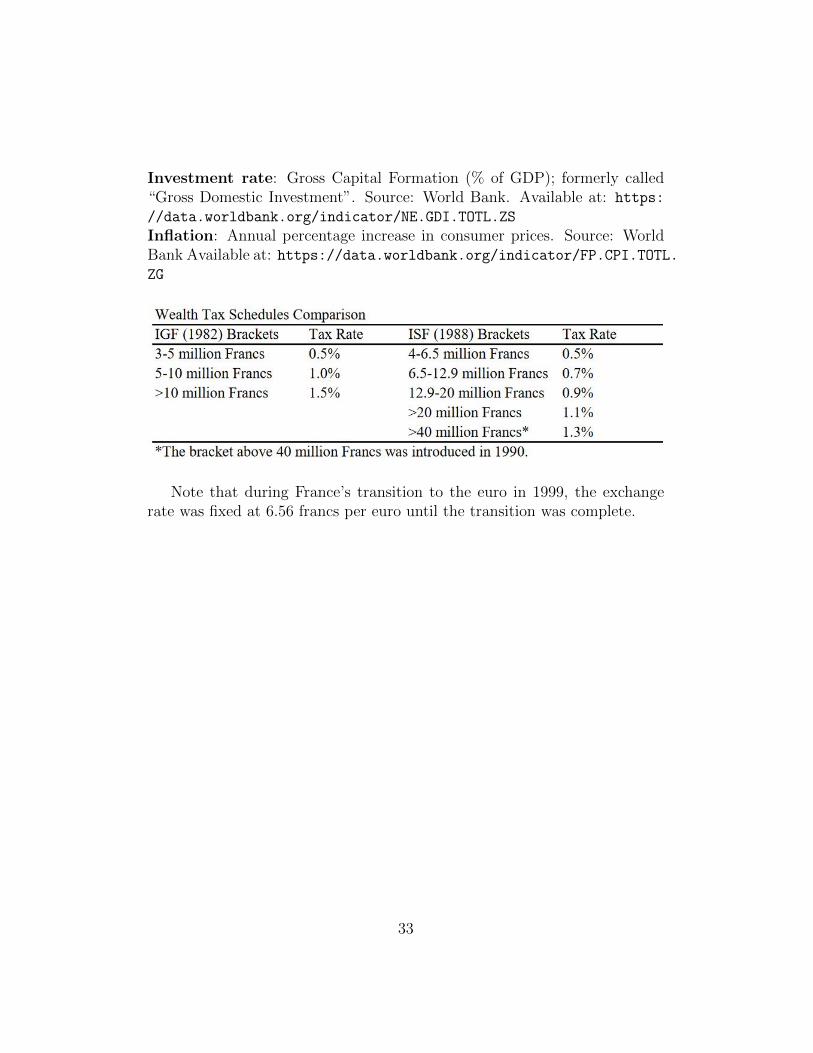
In 1982, France implemented its first individual wealth tax, the Impot sur lesgrandes fortune or “IGF’ (Verbit 1991). To Eric Pichet (2007), the IGF was achiefly ideological policy that aimed to “change life” through redistribution.In 1986, under right-wing prime minister Jacques Chirac, the wealth tax wasrepealed under the auspices of liberalizing the economy. In 1988, socialistsregained the head of government when Michel Rocard began his tenure asprime minister, promptly reimplementing a revised, less radical version ofthe wealth tax, the Impot de solidarite sur la fortune or “ISF.” The ISFremained in effect until 2019. The differences between the tax schedules canbe found in the Appendix.

France was not alone in its full commitment to wealth taxation. In 1990,eleven other OECD countries had active progressive wealth taxes. However,as of 2020, only three of these countries (Switzerland, Spain, and Norway)continue to tax individual wealth (Drometer and et al. 2018).

In recent decades, income and wealth inequality have increased over time.Saez and Zucman (2016) observe that, in the case of the US, increasing wealthinequality is driven by increasing income and saving rate inequality. Piketty,Saez, and Zucman (2018) also find that the inverse is true: increasing in-come inequality has been primarily a capital-driven phenomenon since the1990s. In other words, income inequality and wealth inequality both exacer-bate one another in a positive feedback loop. Increasing economic inequalityis hardly unique to the United States—rising wealth and income inequal-ity has been a global trend since 1980, according to the World InequalityReport 2018. With mounting evidence of increasing economic inequality,wealth taxes have become a popular instrument of choice among policymak-ers around the world. American senators Elizabeth Warren1 and BernieSanders2 proposed wealth taxes during their 2020 presidential campaigns.In 2019, German Social Democrats made steps toward introducing a wealthtax.3 And in 2020, Argentina’s president spoke for a need for wealth redistri-

1Elizabeth Warren, “Ultra Millionaire Tax,” https://elizabethwarren.com/plans/ultra-millionaire-tax

2Bernie Sanders, “Tax on Extreme Wealth,” https://berniesanders.com/issues/tax-extreme-wealth/

3Michael Nienaber, “Germany’s SPD wants to target super rich with wealth tax,Last modified August 26, 2019 https://www.reuters.com/article/us-germany-politics-taxation/germanys-spd-wants-to-target-super-rich-with-wealth-tax-idUSKCN1VG1LZ

2

bution with its Economy Minister explicitly advocating for wealth taxation.4

However, there is some literature purporting the negative effects of awealth tax. The first major criticism is that wealth taxes harm economicgrowth. Hansson (2010) finds that, internationally, each additional percent-age point increase in wealth taxation lowers economic growth modestly—0.02 to 0.04 percentage points per year. Pichet (2007) finds that the ISFdampened economic growth by roughly 0.2 percent per annum in France,using a Cobb-Douglas production function to calculate the effects of capitalflight on growth.

The second criticism is that wealth taxes lead to economic damage throughcapital flight and disincentives to save. Pichet (2007) argues that from1988 to 2007, the ISF caused capital flight equivalent to about 200 billioneuros. Wealthier French “tax refugees” often moved to countries withoutwealth taxes, taking their assets with them. According to Pichet, they of-ten moved to countries like Belgium, which held 63,000 French tax refugeesin 2005. However, Pichet’s approach in calculating his 200 billion euro fig-ure is rather simplistic and flawed— he simply tallies up the number of taxrefugees present in Switzerland (approximately 20,000 at the time of the pa-per) and multiplies it by the average estate size of citizens subject to theISF (about 5 million euros) to yield the rough amount of wealth that left thecountry—100 billion euros. Then, he multiplies this number by two, statingthat “a reasonable number would, therefore, be twice this amount.”

This calculation is problematic for a number of reasons. First, the value ofthe assets owned by tax refugees likely vary over time and, according to Pichethimself, around two taxpayers a day leave France because of the ISF; capitalflight does not occur all at the same time. Secondly, French tax refugeesmay have a different average net worth from those who remain in France tobe taxed by the ISF. And, finally, the choice to only use the number of taxrefugees solely in Switzerland is arbitrary. To Pichet’s credit, there does notexist readily available data with the exact value of per capita wealth of thesetax refugees. Therefore, an analysis that utilizes counterfactuals generatedthrough publicly available macroeconomic data can potentially provide anestimate of capital flight over time without needing this exact data.

Regarding wealth taxation’s effect on savings, wealth taxes are often au-

4Sebastian Boyd, ”Argentina’s Economy Minister Backs Wealth Tax, RejectsAusterity,” https://www.bloomberg.com/news/articles/2020-04-19/argentina-s-economy-minister-backs-wealth-tax-rejects-austerity

3

tomatically assumed to have a negative effect on savings rates. For example,in its article on the negative impacts of capital and wealth taxes, the CatoInstitute simply assumes that wealth taxes negatively impact savings be-haviors, which would negatively affect capital accumulation and, therefore,economic growth.5 Despite claims like these, there are no formal analysesin the literature that quantify the effect that wealth taxes have on savingsrates.

Overall, the literature tends to be speculative of its impacts or faulty incalculating the impacts of wealth taxation in France. Additionally, becausealmost all literature on French wealth taxes focuses on the ISF, there is adearth of analysis on the impact of the IGF, France’s first wealth tax. Theprimary purpose of this paper is to estimate the impacts of the IGF andISF by generating counterfactuals of France through a synthetic controlsmethod. In this paper, I estimate the impacts to economic growth measuredin GDP per adult. I also observe the potential changes in savings behaviorand quantify its impact on wealth per adult. Finally, I attempt to quantifythe overall economic damage of wealth taxation using wealth per adult as anoutcome variable.

2 The Synthetic Controls Method

As Abadie and et al. (2014) explain, the synthetic controls method generatesa counterfactual that is a weighted combination of other countries whoseweights sum to one. This synthetic control draws from a pool of countriesthat represents a control group, which the authors dub the “donor pool.” Thesynthetic controls method draws from this donor pool to create a syntheticversion of the original country. For example, Abadie and et al. (2014) exam-ine the economic effects of the German Reunification in 1990. To generatetheir counterfactual of a West Germany that never reunified with its easterncounterpart, they gather data on the standard predictors of economic growth(e.g. educational attainment, industry share of the economy, and etc.) forWest Germany and the OECD countries in their donor pool. Then, theyassign a weight to each country in their dataset such that two conditionsare met: (1) the differences between the countries in terms of their economicpredictors are minimized and (2) the weights of all countries in the counter-

5Chris Edwards, “Taxing Wealth and Capital Income,” Last modified August 1, 2019.https://www.cato.org/publications/tax-budget-bulletin/taxing-wealth-capital-income

4

factual sum to one. In short, the synthetic controls method aims to generatea counterfactual that best resembles the original country.

Formally, I have a sample of j + 1 units of observation, where j=1 is our“treated unit” (i.e. France) and j = (2, 3, . . . , J + 1) are potential countriesin its synthetic control (i.e. the “donor pool”). In this paper, the donor poolfor France must not have implemented a wealth tax during the pretreatmentand post-treatment periods.

We possess a sample that is a “balanced panel,” a data set where allunits are observed at the same time periods t = (1, 2, . . . , T ). With a posi-tive number of pre-intervention periods (1, 2, ...T0) and post-intervention pe-riods (T0 + 1, . . . , T ), the treated unit is fully exposed to treatment start-ing from T0 + 1. The observed time period spans from 1960-1992 withthe pre-intervention period (1, 2, ...T0) being from 1960-1982 and the post-intervention period (T0 + 1, . . . , T ) being from 1983-1992. This paper’s pe-riod of observation ends in 1992 because, as Abadie and et al. (2014) note,“a roughly decade long period [...] seems like a reasonable limit on the spanof plausible prediction.”

A synthetic control is the weighted average of units in the donor pool—acombination of untreated units. A synthetic control is defined as a (J×1)vector of weight W = (w2, w3, ..., wj+1)′ where 0 ≤ wi ≤ 1. Let X1 be avector containing the values of pre-intervention characteristics of the treatedunit and X0 be a vector containing the values of the same pre-interventioncharacteristics of units in the donor pool. For m = 1, ...k, let the m-th vari-able represent values of the m-th pre-intervention characteristic; there are ktotal pre-intervention characteristics. The weights of units in the syntheticcontrol are selected such that the pre-intervention characteristics between thetreated unit and the synthetic control are minimized. Ultimately, the syn-thetic control minimizes the following expression:

∑km=1 vm(X1m −X0mW )2

This minimization is performed by selecting a weight W for each countryin the donor pool where:

(1) X1 − X0W is the difference between pre-intervention characteristicsof the treated unit and the synthetic control multiplied by the weight of adonor pool country.

(2) vm is the relative importance of a pre-intervention characteristic inpredicting the outcome variable when measuring the discrepancy from ex-pression (1).6

6Practically everything from this general model can be credited to Abadie and et al.

5

Minimizing this expression minimizes “mean root squared predicted er-ror” (MRSPE), the summation of the squared values of annual differencesbetween France and its synthetic control during the pre-intervention period.The solution to this minimization problem is calculated via the Stata package”Synth,” providing country weights in the synthetic control.

For all three synthetic controls I generate on GDP per adult, savingsrates, and wealth per adult, the donor pools draw from OECD countriesthat did not have active net wealth taxes from 1960 to 1992. The 13 coun-tries that meet this requirement are Australia, Belgium, Canada, Greece,Italy, Japan, South Korea, Luxembourg, Mexico, New Zealand, Portugal,the United Kingdom, and the United States.7 This paper’s donor poolsexclude countries that had a wealth tax active during this period, whichincludes Austria, Denmark, Finland, Germany, Iceland, Ireland, the Nether-lands, Norway, Poland, Spain, Sweden, and Switzerland. Due to varyingdata availability, the donor pools are customized for each outcome variableand are described in their respective sections.

While property and bequest taxes do serve as wealth taxes on specifictypes of wealth, this paper focuses on the effect of a more general wealth taxthat France implemented in 1982 and 1988: the net wealth tax on the valueof an individual’s assets minus liabilities. Therefore, countries with propertyand bequest taxes are not excluded from the donor pool.

For the pre-intervention characteristics of GDP per adult, I use the samestandard set of economic growth predictors of countries utilized by Abadieand et al. (2014): GDP per adult,8 trade openness, investment rate, school-ing, industry share of the economy, and inflation. I collect data for tradeopenness, investment rate, and inflation from the World Bank. Data formean years of schooling comes from the Lee and Lee Long-Run EducationalDataset. GDP per adult comes from the World Inequality Database (WID).For the outcome variables of wealth per adult and savings rates, their pre-

(2014)7Israel is excluded due to missing data. Turkey and Chile are excluded due to having

income and wealth significantly lower than other countries in the data pool. Regardless,if these countries are included in the donor pools, they would only be used in the incomeper adult synthetic control; the results do not change with their inclusion.

8Abadie and et al. use GDP per capita. However, GDP per adult is arguably superiorbecause it only includes the working-age population. Using GDP per adult also maintainscontinuity in units used with another outcome variable I study in this paper: wealth peradult.

6

intervention characteristics use some of the same economic predictors as GDPper adult; their pre-intervention characteristics described in detail in theirrespective sections. I collect wealth per adult data from the WID and savingsrates data from the World Bank. Specific details of all economic predictorsand outcome variables along with their respective sources can be located inthe Appendix. This paper’s sample consists of annual panel data composedof country-level aggregated data. The entire dataset spans from 1960 to 2018.

This paper uses its outcome variables as pretreatment characteristics ina specific manner; Abadie and et al. (2014) state that “the preinterventioncharacteristics in X1 and X0 may include pre-intervention values of the out-come variable.” In a separate paper that uses a synthetic control to examinethe impact of California’s tobacco control program, Abadie and et al. (2010)uses its outcome variable, cigarette sales, in specific years as characteristicsin the pretreatment period (i.e. cigarette sales in 1988, 1980, and 1975) tocreate a synthetic control of California that best fits cigarette sales during thepretreatment period. This paper uses a similar method to generate syntheticcontrols for all three outcome variables to best emulate France’s performanceduring the pretreatment period. These selected years are shown in the re-spective section of each outcome variable.

There are a number of advantages to generating a synthetic control as op-posed to using a difference in differences method. First, according to Abadieand et al. (2014) “a combination of comparison units (which we term ‘syn-thetic control’) often does a better job of reproducing the characteristics ofthe unit or units representing the case of interest than any single comparisonunit alone.” Finding a country that closely resembles or parallels France’seconomic performance before its wealth tax can be a matter of trial-and-error. Of all countries I observed in my dataset, there were none that closelyapproximated France during the pretreatment period as closely as the syn-thetic controls I generated. Secondly, there is an advantage in tracking theeffect of multiple treatments over time when using synthetic controls. Thewealth tax was abolished in 1986 and reimplemented in 1988, which wouldnarrow the time frame to analyze the effects of this wealth tax from 1982to 1986 under a difference in differences method. If one wanted to analyzethe effects of the wealth tax after its reimplementation in 1988, there wouldbe a pre-intervention period of only two years (1986 and 1987) that couldhave easily been impacted by the previous treatment period from 1982 to1986 from lagged effects. On the other hand, a synthetic controls methodhas the advantage of generating a counterfactual that can be exposed to

7

multiple treatments over time as long as the initial treatment period is speci-fied, and the donor pool is composed of countries that were never exposed towealth taxation throughout all periods of observation. The synthetic controlof France can be best understood as a France that never dabbled in wealthtaxation at all, never undergoing a wealth tax in 1982, a repeal in 1986, anda re-implementation in 1988.

Finally, a difference in differences method has the unverifiable assump-tion of parallel trends; omitted variables are presumed to remain constantover time. While imperfect, a synthetic controls method has a number ofpotential robustness tests. In this paper, we perform two types of robust-ness tests. First, after generating a synthetic control, similarly to Abadieand et al. (2014), I perform a “leave-one-out” robustness test where I gen-erate synthetic controls by removing all positively-weighted countries fromthe donor pool sequentially. For example, if a synthetic control consists ofthree positively-weighted countries, the leave-one-out robustness test gen-erates three synthetic controls, removing these three countries one-by-one.If these synthetic controls generate similar results to the original syntheticcontrol, the original results are not overly dependent on the availability ofcertain individual countries in the donor pool. Secondly, for GDP per capita,this paper runs what Abadie and et al. (2014) dub “placebo studies.” In asynthetic controls context, performing a placebo test entails performing thesynthetic controls method when treatment did not occur. For GDP per adult,I run an “in-time” placebo test. To run their placebo study for their WestGerman synthetic control, Abadie and et al. (2014) generated synthetic con-trol for West Germany in 1975, even though Germany reunited in 1990 toprove that their original results could be truly be attributed to treatment.Because there is insufficient data for wealth per adult and savings rates, anin-time placebo is inappropriate for these two outcome variables.9

9The data for both wealth per adult and savings rates both start in 1970, not providingenough time to create synthetic controls that resemble France during the pretreatmentperiod.

8

3 GDP Per Adult

3.1 Constructing a Synthetic Control

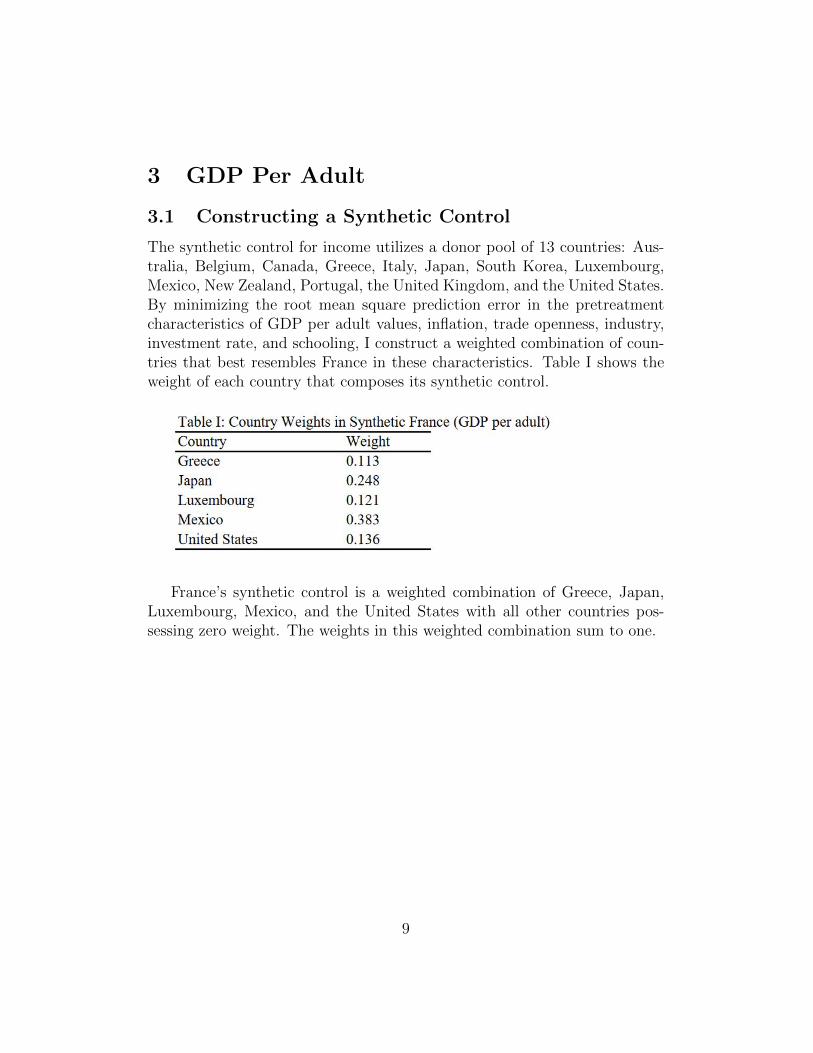
The synthetic control for income utilizes a donor pool of 13 countries: Aus-tralia, Belgium, Canada, Greece, Italy, Japan, South Korea, Luxembourg,Mexico, New Zealand, Portugal, the United Kingdom, and the United States.By minimizing the root mean square prediction error in the pretreatmentcharacteristics of GDP per adult values, inflation, trade openness, industry,investment rate, and schooling, I construct a weighted combination of coun-tries that best resembles France in these characteristics. Table I shows theweight of each country that composes its synthetic control.

France’s synthetic control is a weighted combination of Greece, Japan,Luxembourg, Mexico, and the United States with all other countries pos-sessing zero weight. The weights in this weighted combination sum to one.

9

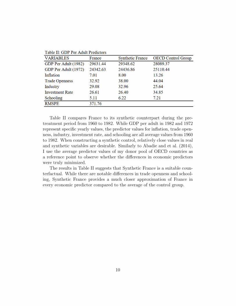
Table II compares France to its synthetic counterpart during the pre-treatment period from 1960 to 1982. While GDP per adult in 1982 and 1972represent specific yearly values, the predictor values for inflation, trade open-ness, industry, investment rate, and schooling are all average values from 1960to 1982. When constructing a synthetic control, relatively close values in realand synthetic variables are desirable. Similarly to Abadie and et al. (2014),I use the average predictor values of my donor pool of OECD countries asa reference point to observe whether the differences in economic predictorswere truly minimized.

The results in Table II suggests that Synthetic France is a suitable coun-terfactual. While there are notable differences in trade openness and school-ing, Synthetic France provides a much closer approximation of France inevery economic predictor compared to the average of the control group.

10

3.2 Wealth Taxation’s Effect on Income

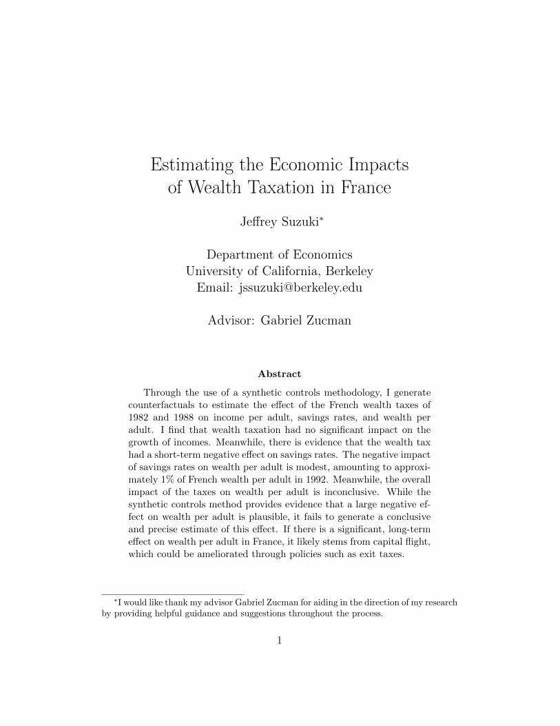
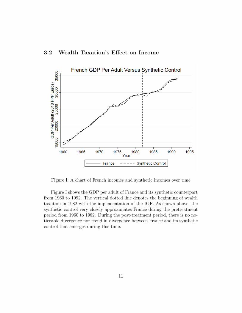
Figure I: A chart of French incomes and synthetic incomes over time

Figure I shows the GDP per adult of France and its synthetic counterpartfrom 1960 to 1992. The vertical dotted line denotes the beginning of wealthtaxation in 1982 with the implementation of the IGF. As shown above, thesynthetic control very closely approximates France during the pretreatmentperiod from 1960 to 1982. During the post-treatment period, there is no no-ticeable divergence nor trend in divergence between France and its syntheticcontrol that emerges during this time.

11

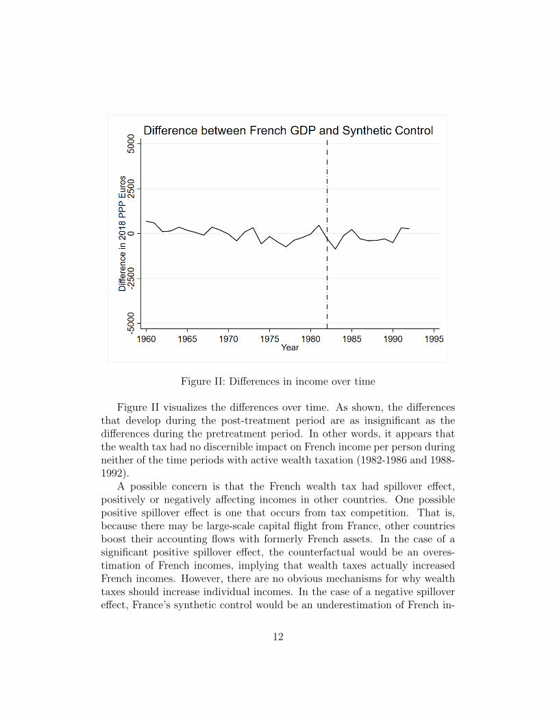
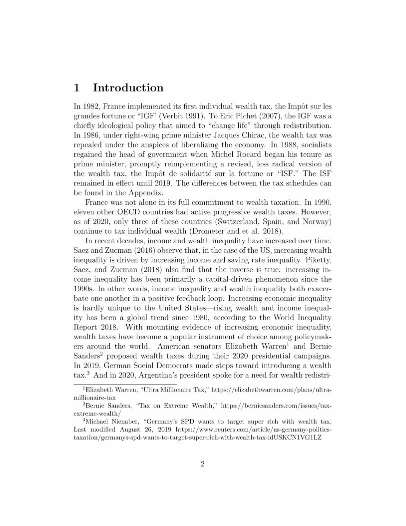
Figure II: Differences in income over time

Figure II visualizes the differences over time. As shown, the differencesthat develop during the post-treatment period are as insignificant as thedifferences during the pretreatment period. In other words, it appears thatthe wealth tax had no discernible impact on French income per person duringneither of the time periods with active wealth taxation (1982-1986 and 1988-1992).

A possible concern is that the French wealth tax had spillover effect,positively or negatively affecting incomes in other countries. One possiblepositive spillover effect is one that occurs from tax competition. That is,because there may be large-scale capital flight from France, other countriesboost their accounting flows with formerly French assets. In the case of asignificant positive spillover effect, the counterfactual would be an overes-timation of French incomes, implying that wealth taxes actually increasedFrench incomes. However, there are no obvious mechanisms for why wealthtaxes should increase individual incomes. In the case of a negative spillovereffect, France’s synthetic control would be an underestimation of French in-

12

comes, implying that wealth taxes decreased incomes. But there are noobvious reasons for why a wealth tax would negatively affect the incomes ofother countries in a significant way.

If there is a significant spillover effect from the wealth tax that impactsthe per adult incomes of the countries that compose this synthetic control(Greece, Japan, Luxembourg, Mexico, and the United States), the wealthtax may have had an effect on incomes. A weakness of a synthetic controlsmethod is that spillover effects cannot be accounted for.

13

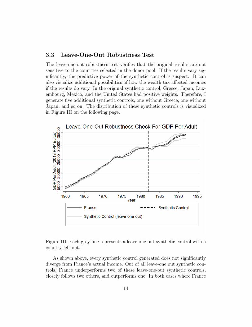
3.3 Leave-One-Out Robustness Test

The leave-one-out robustness test verifies that the original results are notsensitive to the countries selected in the donor pool. If the results vary sig-nificantly, the predictive power of the synthetic control is suspect. It canalso visualize additional possibilities of how the wealth tax affected incomesif the results do vary. In the original synthetic control, Greece, Japan, Lux-embourg, Mexico, and the United States had positive weights. Therefore, Igenerate five additional synthetic controls, one without Greece, one withoutJapan, and so on. The distribution of these synthetic controls is visualizedin Figure III on the following page.

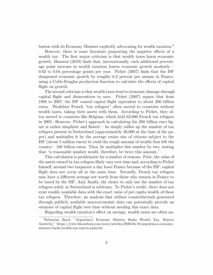
Figure III: Each grey line represents a leave-one-out synthetic control with acountry left out.

As shown above, every synthetic control generated does not significantlydiverge from France’s actual income. Out of all leave-one out synthetic con-trols, France underperforms two of these leave-one-out synthetic controls,closely follows two others, and outperforms one. In both cases where France

14

underperforms two synthetic controls, French adults earned 850 euros a yearless compared to their synthetic counterparts in 1992. This difference repre-sents about 2% of French incomes. Therefore, it is possible that the wealthtax had a modest negative effect on French incomes. However, given thatthere are three other synthetic controls that either show lack of impact or apositive impact, this modest negative effect on French incomes is, at best,speculative. Nevertheless, the fact that all leave-one-out robustness testsfall within a relatively narrow range of 1000 euros ( 3% of French income)throughout all treatment periods reinforces shows that the results are notvery sensitive to the donor pool.

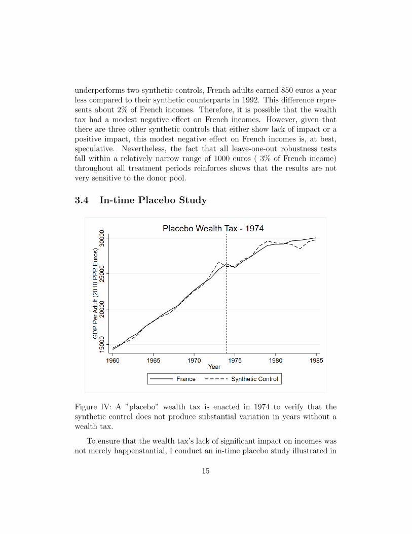
3.4 In-time Placebo Study

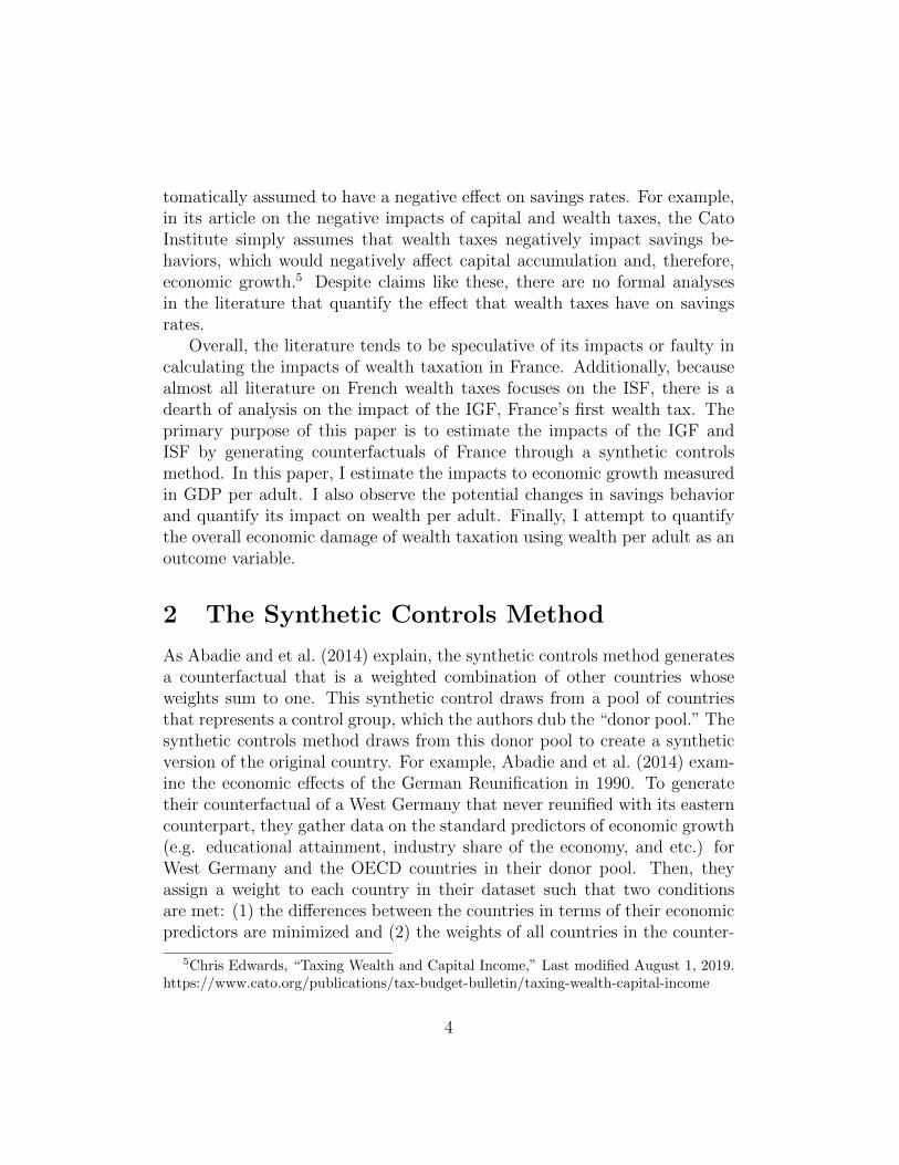
Figure IV: A ”placebo” wealth tax is enacted in 1974 to verify that thesynthetic control does not produce substantial variation in years without awealth tax.

To ensure that the wealth tax’s lack of significant impact on incomes wasnot merely happenstantial, I conduct an in-time placebo study illustrated in

15

Figure IV. Rather than conventionally using an in-time placebo to verify thatan impact of treatment is reliant on the time of treatment as Abadie and etal. (2014) would, I use an in-time placebo to verify that the wealth tax wouldhave had as much impact as not implementing it under this synthetic control.If the in-time placebo study shows no substantial divergences between Franceand its synthetic control, it further proves that the results of the originalsynthetic control are valid. The in-time placebo study is set in 1974, eightyears before the wealth tax was implemented in 1982. The rationale behindselecting 1974 as the year of the placebo study is that it is the most distantpretreatment year from 1982 that has the most predictor data available.

In the above in-time placebo study, France and its synthetic control arelargely similar during the pretreatment period. During the post-treatmentperiod, two minor gaps form in 1978 and 1983. The negative gap in 1978is about 650.04 euros (about 2.3% of French GDP at the time), while thepositive gap in 1983 is about 1219.91 euros (about 4.1% of French GDP atthe time). Because these gaps are ephemeral and small, they do not formany substantial trends where France underperforms and overperforms its syn-thetic counterpart. This placebo study verifies that a wealth tax has as mucheffect on income as not implementing a wealth tax under this synthetic con-trols study; the effect of a wealth tax on incomes is either nil or insignificant.

Overall, accounting for the narrow range of leave-one-out synthetic con-trols and placebo study results, the argument that French incomes were neg-atively affected by wealth taxes in a significant way during the 1982-1992period is implausible. If there is an effect, it is far too small to observe orrequires more than a decade for the effect to manifest significantly.

A natural question that arises is whether these wealth taxes had a nega-tive effect on wealth accumulation. Given that the wealth tax had no effecton the growth of incomes, it is worthwhile to explore how French residentssaved this income differently after the passage of these wealth taxes.

16

4 Savings Rate

4.1 Constructing a Synthetic Control

A synthetic control may reveal a potential effect of wealth taxes on the savingsrates of French income earners. Additionally, if there is a negative effecton savings, a drop in savings rate could be used to quantify an negativeeffect on wealth accumulation. With savings as a percentage of GDP as theoutcome variable of interest, this synthetic control utilizes a donor pool of 12countries: Australia, Belgium, Canada, Greece, Italy, Japan, Luxembourg,Mexico, New Zealand, Portugal, the United States, and the United Kingdom.

I use three predictors for savings rates: GDP per adult, investment rate,and schooling. First, for GDP per adult, the amount of individual income in-fluences savings behavior. Higher income earners tend to consume a smallerproportion of their income, as their marginal propensity to consume decreaseswith increasing income. This lower consumption translates to a higher sav-ings rate. Secondly, for investment rate, the rationale is that investmentrates are usually very close to savings rates; people usually invest their sav-ings. Therefore, investment rates are likely to be useful in predicting savingsrates, even if they do not have a causal relationship. Finally, I use meanyears of schooling as the final predictor. Cole and et al. (2012) find that ad-ditional years of schooling positively predicted individual savings behavior inthe United States. Bingley and Martinello (2017) observe that, in Denmark,more years of schooling increases wealth accumulation toward retirement.

Because savings rates often experience 1-2 percentage point fluctuationsfrom year-to-year, fluctuations of 10-20 percent in savings rates occur year-to-year in any given country.10 These large fluctuations make it practicallyimpossible to create a synthetic control that closely approximates Frenchsavings rates every year during the pretreatment period. To “smooth out”these fluctuations, I instead utilize a three year moving average of Frenchsavings rates.11 The advantage of using a moving average is that it allows asynthetic control to resemble France during the pretreatment period. How-

10To be precise, changes in percentage points are different from percent changes. Forinstance, a 2 percentage point change in a 20 percent savings rate represents a 10 percentchange in savings rates.

11A three year moving average entails averaging values at a specific year n and its twoconsecutive prior years (n − 1) and (n − 2) for all years n. For example, the three yearmoving average for savings rate in 1980 is the mean of the savings rates of 1980, 1979, and1978.

17

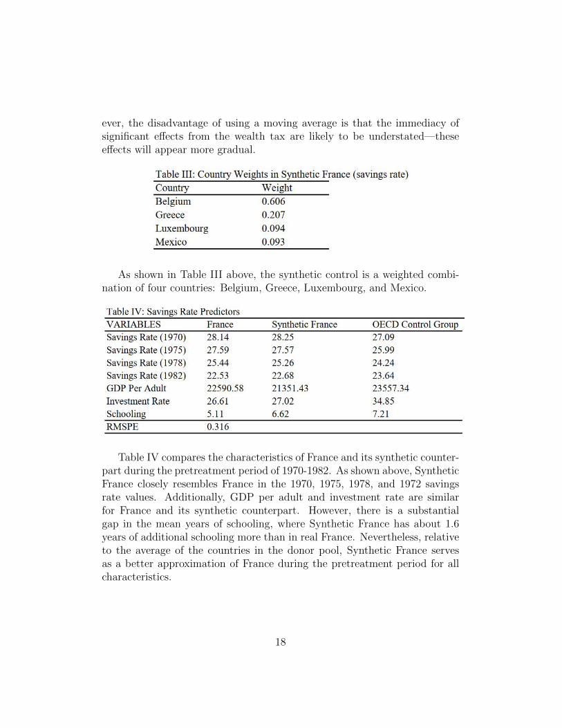
ever, the disadvantage of using a moving average is that the immediacy ofsignificant effects from the wealth tax are likely to be understated—theseeffects will appear more gradual.

As shown in Table III above, the synthetic control is a weighted combi-nation of four countries: Belgium, Greece, Luxembourg, and Mexico.

Table IV compares the characteristics of France and its synthetic counter-part during the pretreatment period of 1970-1982. As shown above, SyntheticFrance closely resembles France in the 1970, 1975, 1978, and 1972 savingsrate values. Additionally, GDP per adult and investment rate are similarfor France and its synthetic counterpart. However, there is a substantialgap in the mean years of schooling, where Synthetic France has about 1.6years of additional schooling more than in real France. Nevertheless, relativeto the average of the countries in the donor pool, Synthetic France servesas a better approximation of France during the pretreatment period for allcharacteristics.

18

4.2 Wealth Taxation’s Effect on Savings Rates

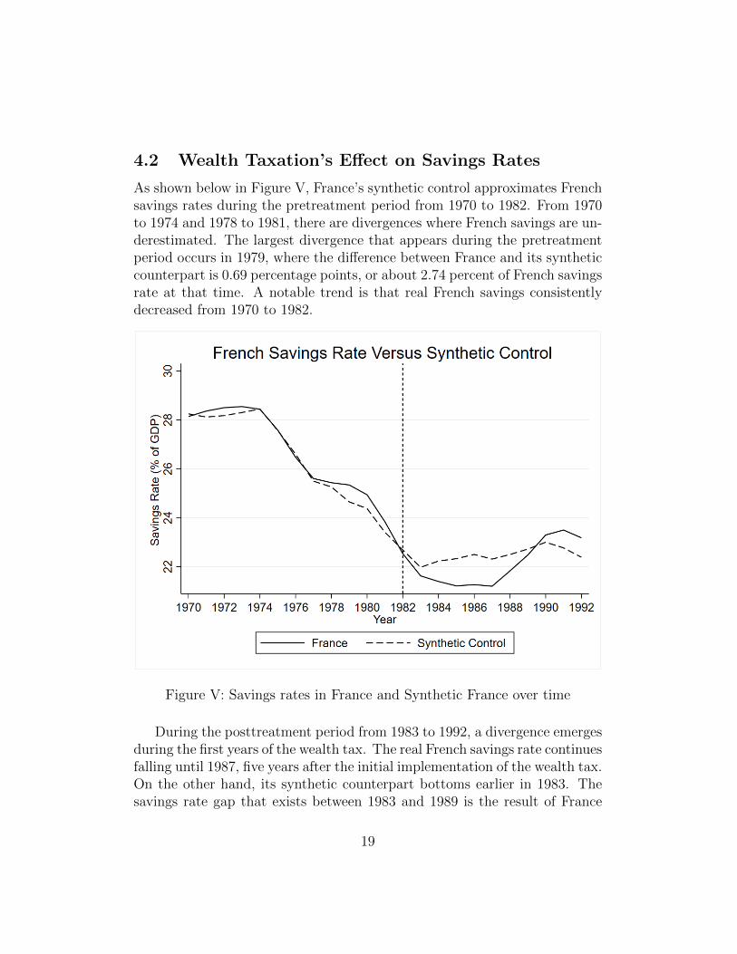
As shown below in Figure V, France’s synthetic control approximates Frenchsavings rates during the pretreatment period from 1970 to 1982. From 1970to 1974 and 1978 to 1981, there are divergences where French savings are un-derestimated. The largest divergence that appears during the pretreatmentperiod occurs in 1979, where the difference between France and its syntheticcounterpart is 0.69 percentage points, or about 2.74 percent of French savingsrate at that time. A notable trend is that real French savings consistentlydecreased from 1970 to 1982.

Figure V: Savings rates in France and Synthetic France over time

During the posttreatment period from 1983 to 1992, a divergence emergesduring the first years of the wealth tax. The real French savings rate continuesfalling until 1987, five years after the initial implementation of the wealth tax.On the other hand, its synthetic counterpart bottoms earlier in 1983. Thesavings rate gap that exists between 1983 and 1989 is the result of France

19

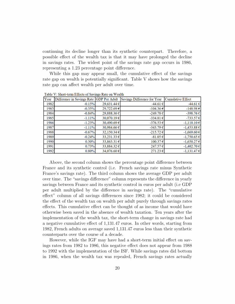
continuing its decline longer than its synthetic counterpart. Therefore, apossible effect of the wealth tax is that it may have prolonged the declinein savings rates. The widest point of the savings rate gap occurs in 1986,representing a 1.23 percentage point difference.

While this gap may appear small, the cumulative effect of the savingsrate gap on wealth is potentially significant. Table V shows how the savingsrate gap can affect wealth per adult over time.

Above, the second column shows the percentage point difference betweenFrance and its synthetic control (i.e. French savings rate minus SyntheticFrance’s savings rate). The third column shows the average GDP per adultover time. The “savings difference” column represents the difference in yearlysavings between France and its synthetic control in euros per adult (i.e GDPper adult multiplied by the difference in savings rate). The “cumulativeeffect” column of all savings differences since 1982; it could be consideredthe effect of the wealth tax on wealth per adult purely through savings rateseffects. This cumulative effect can be thought of as income that would haveotherwise been saved in the absence of wealth taxation. Ten years after theimplementation of the wealth tax, the short-term change in savings rate hada negative cumulative effect of 1,131.47 euros. In other words, starting from1982, French adults on average saved 1,131.47 euros less than their syntheticcounterparts over the course of a decade.

However, while the IGF may have had a short-term initial effect on sav-ings rates from 1982 to 1986, this negative effect does not appear from 1988to 1992 with the implementation of the ISF. While savings rates did bottomin 1986, when the wealth tax was repealed, French savings rates actually

20

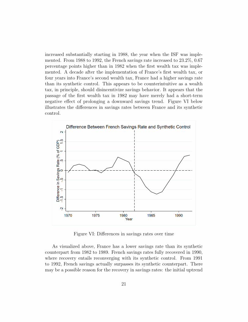
increased substantially starting in 1988, the year when the ISF was imple-mented. From 1988 to 1992, the French savings rate increased to 23.2%, 0.67percentage points higher than in 1982 when the first wealth tax was imple-mented. A decade after the implementation of France’s first wealth tax, orfour years into France’s second wealth tax, France had a higher savings ratethan its synthetic control. This appears to be counterintuitive as a wealthtax, in principle, should disincentivize savings behavior. It appears that thepassage of the first wealth tax in 1982 may have merely had a short-termnegative effect of prolonging a downward savings trend. Figure VI belowillustrates the differences in savings rates between France and its syntheticcontrol.

Figure VI: Differences in savings rates over time

As visualized above, France has a lower savings rate than its syntheticcounterpart from 1982 to 1989. French savings rates fully recovered in 1990,where recovery entails reconverging with its synthetic control. From 1991to 1992, French savings actually surpasses its synthetic counterpart. Theremay be a possible reason for the recovery in savings rates: the initial uptrend

21

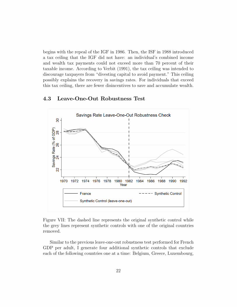
begins with the repeal of the IGF in 1986. Then, the ISF in 1988 introduceda tax ceiling that the IGF did not have: an individual’s combined incomeand wealth tax payments could not exceed more than 70 percent of theirtaxable income. According to Verbit (1991), the tax ceiling was intended todiscourage taxpayers from “divesting capital to avoid payment.” This ceilingpossibly explains the recovery in savings rates. For individuals that exceedthis tax ceiling, there are fewer disincentives to save and accumulate wealth.

4.3 Leave-One-Out Robustness Test

Figure VII: The dashed line represents the original synthetic control whilethe grey lines represent synthetic controls with one of the original countriesremoved.

Similar to the previous leave-one-out robustness test performed for FrenchGDP per adult, I generate four additional synthetic controls that excludeeach of the following countries one at a time: Belgium, Greece, Luxembourg,

22

and Mexico. The results of this leave-one-out robustness test is visualizedabove in Figure VII.

As shown above, France saved less than all of its synthetic counterpartsbetween 1982 and 1989—a similar result to the original synthetic control.This corroborates the hypothesis that the IGF in 1982 may have prolongedthe savings rate decline. However, there are differences between syntheticcontrols in the size of the gap from 1982 to 1989 and the ending savingsrates in 1992. First, the size of the 1982-1989 gap for all leave-one outsynthetic controls, except for one, is larger than the original synthetic controlgap. This implies that the negative effect on savings rates could have beenlarger than originally estimated. Secondly, while France saves more than itscounterfactual starting from 1990 in the original results, one of the leave-one-out synthetic controls ends with a higher savings rate than France in 1992,implying that French savings rates may have not fully recovered. However,three other leave-one-out synthetic controls corroborate the original findingsthat there was a full savings rate recovery.

This leave-one-out robustness test does verify the existence of the 1982-1989 gap. In fact, every leave-one-out synthetic control except for one hasa wider gap during this time period. It also confirms that wealth taxation’seffect on savings rates translated to a negative effect on wealth per adult,since all of the leave-one-out synthetic controls show either a similarly sizedsavings gap or larger savings gaps than in the original result. Overall, therobustness test verifies the original findings that the wealth tax had a short-term negative effect on savings, which marginally decreased wealth per adultin France. This leaves capital flight as the other potential factor in losingwealth per adult. I attempt to quantify this capital flight effect through athird synthetic control.

23

5 Wealth Per Adult

5.1 Constructing a Synthetic Control

To generate a synthetic control for wealth, I use a method very similar togenerating one for income. In fact, I use an identical set of economic predic-tors for wealth: trade openness, investment rate, schooling, industry shareof the economy, and inflation. The reasoning behind this is simple: becauseincome is a flow variable, it inextricably affects wealth as a stock variable.In fact, in my dataset, the correlation between income and wealth per adultis 0.82, suggesting that the economic predictors for income would likely workfor wealth as well.

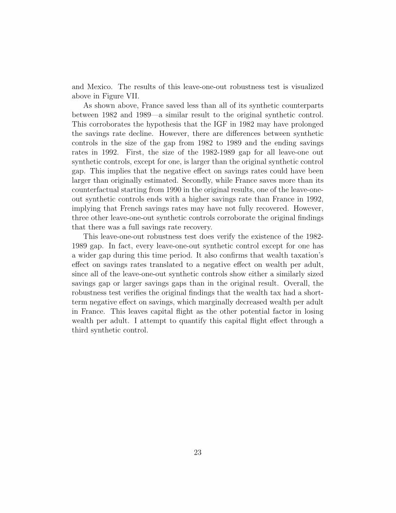
Due to the limitations in data, the donor pool for generating a SyntheticFrance that tracks wealth per adult is smaller than the one that tracks in-come. In general, there is far less wealth per adult data than income peradult data. To ensure that there is at least 10 years of pretreatment data, Iinclude all countries with wealth per adult that have data from at least 1972onward. This leaves a donor pool of seven countries: Australia, Canada,Italy, Japan, Greece, the United States, and the United Kingdom. Whileit is preferable to have a larger donor pool because larger donor pools gen-erally decrease RMSPE and hypothetically increase the predictive potentialof synthetic controls, it is possible to generate synthetic controls that utilizesmaller donor pools. For instance, Harwell and et al. (2019) utilize donorpools of seven countries to generate synthetic controls to estimate the effectsof a country’s discovery of natural resources on income inequality.

As shown in Table VI above, the synthetic control is a weighted combi-nation of four countries: Canada, Italy, Japan, and the United States.

24

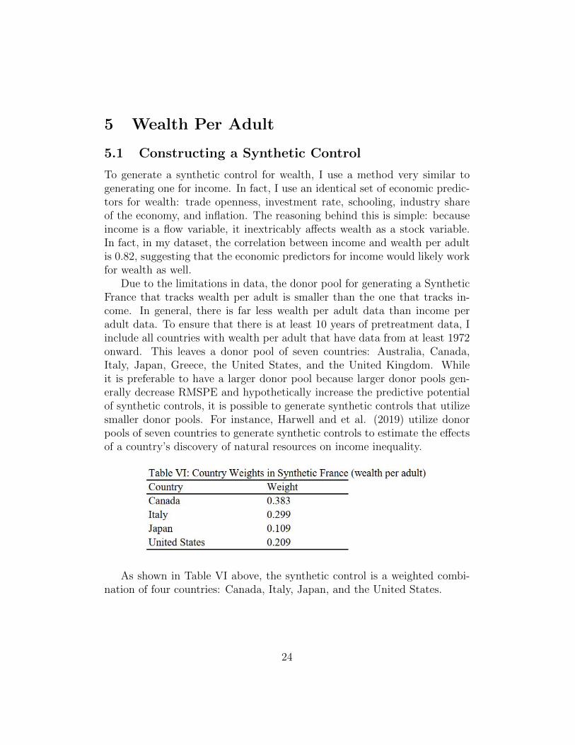
The results in Table VII compares France’s, synthetic France’s, and theOECD control group’s pretreatment characteristics. Compared to the aver-age of the control group, synthetic France provides a closer approximationof France in every economic predictor. The RMSPE is notably higher thanthe RMPSE of the first income synthetic control, which had a RMSPE of371.76. This synthetic control is an inferior approximation of France duringthe pretreatment period and is likely to have less predictive power than thefirst synthetic control to approximate French income. Nevertheless, relativeto the control group on average, it serves as a much better approximation.

25

5.2 Wealth Taxation’s Effect on Wealth per Adult

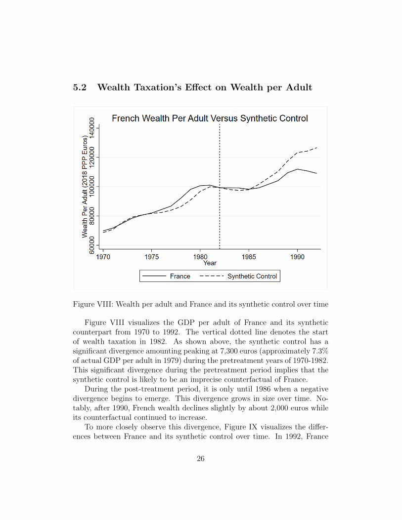
Figure VIII: Wealth per adult and France and its synthetic control over time

Figure VIII visualizes the GDP per adult of France and its syntheticcounterpart from 1970 to 1992. The vertical dotted line denotes the startof wealth taxation in 1982. As shown above, the synthetic control has asignificant divergence amounting peaking at 7,300 euros (approximately 7.3%of actual GDP per adult in 1979) during the pretreatment years of 1970-1982.This significant divergence during the pretreatment period implies that thesynthetic control is likely to be an imprecise counterfactual of France.

During the post-treatment period, it is only until 1986 when a negativedivergence begins to emerge. This divergence grows in size over time. No-tably, after 1990, French wealth declines slightly by about 2,000 euros whileits counterfactual continued to increase.

To more closely observe this divergence, Figure IX visualizes the differ-ences between France and its synthetic control over time. In 1992, France

26

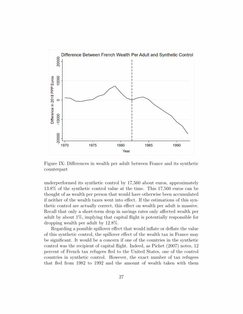
Figure IX: Differences in wealth per adult between France and its syntheticcounterpart

underperformed its synthetic control by 17,560 about euros, approximately13.8% of the synthetic control value at the time. This 17,560 euros can bethought of as wealth per person that would have otherwise been accumulatedif neither of the wealth taxes went into effect. If the estimations of this syn-thetic control are actually correct, this effect on wealth per adult is massive.Recall that only a short-term drop in savings rates only affected wealth peradult by about 1%, implying that capital flight is potentially responsible fordropping wealth per adult by 12.8%.

Regarding a possible spillover effect that would inflate or deflate the valueof this synthetic control, the spillover effect of the wealth tax in France maybe significant. It would be a concern if one of the countries in the syntheticcontrol was the recipient of capital flight. Indeed, as Pichet (2007) notes, 12percent of French tax refugees fled to the United States, one of the controlcountries in synthetic control. However, the exact number of tax refugeesthat fled from 1982 to 1992 and the amount of wealth taken with them

27

is unknown. Nevertheless, there is a distinct possibility that capital flightfrom France increased the average wealth per adult of the United States,suggesting that the synthetic control may overestimate the negative effect ofthe wealth tax.

Because of the synthetic control’s suspect predictive power and concernsof a spillover effect, accepting that the lost wealth per adult is precisely17,560 euros would be hamfisted. A leave-one-out robustness test must beconducted to verify this negative effect.

5.3 Leave-One-Out Robustness Test

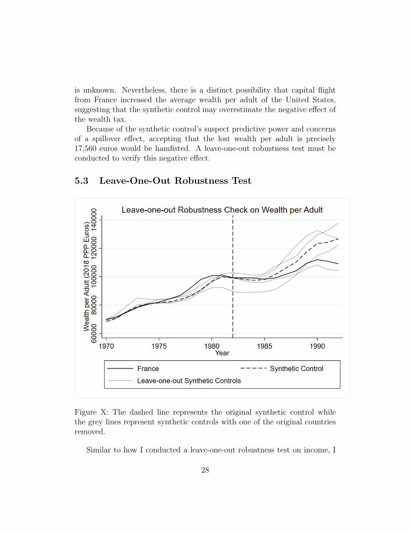
Figure X: The dashed line represents the original synthetic control whilethe grey lines represent synthetic controls with one of the original countriesremoved.

Similar to how I conducted a leave-one-out robustness test on income, I

28

generate four additional synthetic controls, removing one country at a timecontained in the original synthetic control: Canada, Italy, Japan, and theUnited States.

As illustrated above in Figure X, France underperforms every leave-one-out synthetic control in addition to the original synthetic control, except forone. France outperforms the leave-one-out synthetic control that excludesthe United States—wealthiest country in the dataset. Additionally, this par-ticular synthetic control very poorly approximates French wealth per adultduring the pretreatment period, implying that the original synthetic controlis likely overdependent on the United States existing in its donor pool. Theloss of 13.8 percent of wealth per adult over a decade is not a robust result.

Given that there are three leave-one-out synthetic controls, along with theoriginal synthetic control, which hypothetically has the most predictive powerdue to having the most data to better minimizes differences between Franceand synthetic France, a significant negative effect is still highly plausible. Thepresent existence hundreds of thousands of French tax refugees12 in France’sneighboring countries corroborates this plausibility. However, the originalestimate of 17,560 euros lost per adult should not be considered a preciseor reliable estimate. Overall, the synthetic controls method is incapable ofproviding a precise and robust result with the data that currently exists. Themost loss to wealth per adult that can be confirmed is the 1 percent negativeeffect that stems from the short-term negative effect on savings rates.

12As previously stated, there were roughly 63,000 French tax refugees living in Belgiumin 2005. Pichet (2007), using numbers from the French Tax Directorate, states that Bel-gium holds 18% of all fiscal expatriates. It is likely that there were hundreds of thousandsof tax refugees around the world by the time the wealth tax was repealed in 2019.

29

6 Significance of Results and Implications

The main goal of this paper is to test the plausibility of the purported neg-ative economic impacts of the French wealth tax. These two main criticismswere that (1) wealth taxes lower economic growth and (2) wealth taxes leadto economic damage through capital flight and discouraged savings behavior.

If GDP growth is considered synonymous with economic growth, as isoften the case, the synthetic controls method shows that that the wealth taxhad no significant impacts on economic growth, a robust result given bothof the robustness tests performed. This result is significant— even withoutadditional exit taxes or other punitive measures to prevent capital flight, theFrench wealth taxes appeared to have no penalty to economic growth.

Out of the results of all three outcome variables, this lack of impact onincomes is the most robust outcome and arguably has the most importantpolicy implications. Often, wealth taxation is often framed as a pursuit forfairness and equality at the expense of economic growth. However, the syn-thetic controls method provides evidence that this tradeoff is insubstantial.Even if there was large-scale capital flight in France from 1982 to 1992, it didnot significantly impact economic growth. If this lack of effect can be con-firmed across multiple countries, policymakers can implement wealth taxeswithout the fear of hindering economic development.

As for the possible economic damage inflicted on French wealth per adult,the only confirmed effect is a short-term decline in savings rates before aspeedy recovery. This loss in savings had a cumulative effect equivalent to1% of French wealth per adult. Not only is this loss in wealth quite small overthe course of a decade, but the synthetic controls method provides evidencethat wealth taxation did not have a long-term effect on savings behavior. Ifthere is a more substantial negative effect on wealth, it would likely stemfrom capital flight as there are hundreds of thousands of French tax refugeesscattered across the world.

In attempting to quantify this effect, I discovered that a synthetic controlsmethod is insufficient to precisely estimate this capital flight. The methodprovided evidence that a large negative effect on average wealth per adult isplausible through the leave-one-out robustness test. Estimations of this largenegative effect, however, are tenuous. If there was enough data to includemore pretreatment years and countries in the donor pool, there would likelybe a more precise and robust result.

Nevertheless, to combat the potentially large effect of capital flight, pol-

30

icymakers intent on implementing a wealth tax should prioritize append-ing obstacles to disincentivize expatriation. For instance, Senators BernieSanders13 and Elizabeth Warren14 supplemented their wealth tax proposalswith exit taxes of 40-60% and 40% respectively, steeply penalizing expatri-ates attempting to avoid the wealth tax. As Saez and Zucman (2019) note,“the threat of expatriation is primarily a policy variable” rather than an in-evitable outcome of wealth taxation; for example, in the United States, thereis already the precedent of an exit tax that exists for unrealized capital gains,applying to those with incomes over 160,000 dollars or net wealths above 2million dollars. As Pichet (2007) notes, in the 2000s, the repeal of the exittax in France caused a sharp and immediate increase in capital flight, imply-ing that the exit tax was effective before its repeal.15 If governments neednot worry about declines in economic growth or savings, they can address thelast major concern of wealth taxation by sufficiently disincentivizing capitalflight.

13Bernie Sanders, “Tax on Extreme Wealth,” https://berniesanders.com/issues/tax-extreme-wealth/

14Elizabeth Warren, “Ultra Millionaire Tax,” https://elizabethwarren.com/plans/ultra-millionaire-tax

15To be clear, this exit tax was passed in the late 90s. There was no exit tax in placeduring the time frame of my analysis.

31

Appendix

Description and Sources of Variables:GDP Per Adult: Gross Domestic Product per adult denoted in 2018PPP euros. Source: World Inequality Database. Available at: https:

//wid.world/

Wealth Per Adult: the average net assets per adult denoted in 2018 PPPeuros. Source: World Inequality DatabaseSavings Rates: Gross domestic savings as a percentage of GDP. Source:World Bank. Available at: https://data.worldbank.org/indicator/NY.

GDS.TOTL.ZS?locations=FR

Educational attainment: Mean years of education. Source: the Lee andLee Long-Run Educational Dataset. Available at: http://barrolee.com/

Lee_Lee_LRdata_dn.htm

Industry Share: Industry share of the economy expressed as a percentageof GDP. Source: World Bank and World Bank Archival Data. This vari-able uses a myriad of World Bank Archival Data because the most recentversion of the data set has omitted data from past years. The list belowshows where every country’s data is from in this variable. Available at:https://data.worldbank.org/indicator/NV.IND.TOTL.ZS and https://

databank.worldbank.org/source/wdi-database-archives-(beta)#.France- recent 2019 dataAustralia- April 2000 archival dataBelgium- November 2014 archival dataCanada- November 2014 archival dataGreece- October 2012 archival dataItaly- November archival 2014Japan- November archival 2017Korea- recent 2019 dataLuxembourg- November archival 2017Mexico- recent 2019 dataNew Zealand- recent 2019 dataPortugal- November archival 2014United States- November archival 2014 dataUnited Kingdom- November archival 2014 data

Trade Openness: A country’s trade as a percentage of GDP. Source: WorldBank. Available at: https://data.worldbank.org/indicator/NE.TRD.

GNFS.ZS

32

Investment rate: Gross Capital Formation (% of GDP); formerly called“Gross Domestic Investment”. Source: World Bank. Available at: https:

//data.worldbank.org/indicator/NE.GDI.TOTL.ZS

Inflation: Annual percentage increase in consumer prices. Source: WorldBank Available at: https://data.worldbank.org/indicator/FP.CPI.TOTL.ZG

Note that during France’s transition to the euro in 1999, the exchangerate was fixed at 6.56 francs per euro until the transition was complete.

33

References

Abadie, Alberto, Alexis Diamond, and Jens Hainmueller (2014). “Comparative Politics and the

Synthetic Control Method.” American Journal of Political Science 59, no. 2: 495–510.

Abadie, Alberto, Alexis Diamond, and Jens Hainmueller (2010). “Synthetic Control Methods for

Comparative Case Studies: Estimating the Effect of California’s Tobacco Control

Program.” Journal of the American Statistical Association 105(490): 493–505.

Alvaredo, Facundo, Lucas Chancel, Thomas Piketty, Emmanuel Saez, and Gabriel Zucman

(2018). “World Inequality Report,” available at https://wir2018.wid.world/

Bingley, Paul, Alessandro Martinello (2017). “The Effects of Schooling on Wealth

Accumulation Approaching Retirement,” available at:

https://project.nek.lu.se/publications/ workpap/papers/wp17_9.pdf

Cole, Shawn, Anna Paulson, and Gauri Kartini Shastry (2012). “Smart Money: The Effect of

Education on Financial Behavior.” Available at: http://academics.wellesley.edu/

Economics/gshastry/cole-paulson-shastry-financial%20behavior.pdf

Drometer, Marcus et al. (2018) : Wealth and Inheritance Taxation: An Overview and Country

Comparison, ifo DICE Report, ISSN 2511-7823, ifo Institut - Leibniz-Institut für

Wirtschaftsforschung an der Universität München, München, Vol. 16, Iss. 2, pp.45-54

Edwards, Chris, “Taxing Wealth and Capital Income,” Last modified August 1, 2019.

https://www.cato.org/publications/tax-budget-bulletin/taxing-wealth-capital-income

Hansson, Asa (2002). “The Wealth Tax and Economic Growth,” available at:

https://www.researchgate.net/publication/5096483_The_Wealth_Tax_and_Economic_Gr

owth

Hartwell and et al. (2019). “Natural Resources and Income Inequality in Developed Countries:

Synthetic Control Method Evidence,” available at

https://econpapers.repec.org/paper/ostwpaper/381.htm.

Nienaber, Michael “Germany’s SPD wants to target super rich with wealth tax, Last modified

August 26, 2019, https://www.reuters.com/article/us-germany-politics-taxation/

germanys-spd-wants-to-target-super-rich-with-wealth-tax-idUSKCN1VG1LZ

Pichet, Eric (2007). “The Economic Consequences of the French Wealth Tax.” La Revue De

Droit Fiscal. n° 14-5

Piketty, Thomas, Emmanuel Saez, and Gabriel Zucman (2018). “Distributional National

Accounts: Methods and Estimates for the United States.” The Quarterly Journal of

Economics 133, no. 2

Saez, Emmanuel, and Gabriel Zucman (2016). “Wealth Inequality in the United States since

1913: Evidence from Capitalized Income Tax Data,” The Quarterly Journal of

Economics, vol 131(2), pages 519-578.

Saez, Emmanuel, and Gabriel Zucman (2019). “Progressive Wealth Taxation,” available at

http://gabriel-zucman.eu/files/SaezZucman2019BPEA.pdf.

Sanders, Bernie “Tax on Extreme Wealth,” https://berniesanders.com/issues/tax-extreme-wealth/

Verbit, Gilbert Paul (1991). “France Tries a Wealth Tax .” U. Pa. J. Int'l Bus. L. 12

Warren, Elizabeth, “Ultra Millionaire Tax,” available at

https://elizabethwarren.com/plans/ultra-millionaire-tax