Embed Size (px)
Citation preview

Wealth inequality measurement:Methods and evidence from HFCS
Philippe Van KermUniversity of Luxembourg & Luxembourg Institute of Socio-Economic Research
15th Winter School on Inequality and Social Welfare Theory (IT15)
Alba di Canazei, January 14 2020


Outline
Measuring household wealth inequality.How different is it from income inequality measurement?
1. Cowell and Van Kerm (2015), ‘Wealth inequality: A survey’, Journal of EconomicSurveys, 29(4), 671–710.
2. Cowell et al. (2017), ‘Wealth, Top Incomes and Inequality’, in “Wealth: Economicsand Policy”, K. Hamilton and C. Hepburn (Eds.), Oxford University Press.
3. Chauvel et al. (2019), ‘Income and Wealth Above the Median: NewMeasurements and Results for Europe and the United States’, in “What drivesinequality?”, K. Decancq and P. Van Kerm (Eds.), Research on EconomicInequality vol. 27, Emerald Publishing.

Outline
Four themes
1. Equivalence scales
2. Negative net worth
3. Age, life-cycle accumulation and wealth inequality
4. Inference

Outline
What is important but not covered?
1. Data collection methods: surveys vs. administrative/tax sources vs. ‘indirect’methods
2. Components of household net worth (marketable wealth? incl. public pensions?incl. human capital?)
3. Valuation of (real) assets

Two sources of micro-data on wealth (and income)
• ECB Household Finance and Consumption Survey (HFCS); waves 1 (about 2011)and 2 (about 2014); wave 3 (available soon)https://www.ecb.europa.eu/pub/economic-research/research-networks/html/
researcher_hfcn.en.html
All Eurozone countries
• Luxembourg Wealth Study (LWS)http://www.lisdatacenter.org
Many of HFCS datasets along with WAS (for UK) and SCF (for US) in harmonizedform

Let’s fix ideas first

Wealth aggregates
(Kuhn and Ríos-Rull, 2016)
Mean and median wealth across countries

Net wealth composition
USA
DebtsNet worth
Financial assets
Main residence
Other real assets
Self-employment business
6.4 1.3 1.3
2.3
1.3
1.2
2.9
UK
DebtsNet worth
Financial assets
Main residence
Other real assets
Self-employment business
6.0 1.1 1.1
3.8
1.4
0.5
1.4

Net wealth composition
France
DebtsNet worth
Financial assets
Main residence
Other real assets
Self-employment business
6.3 0.7 0.7
3.3
1.7
0.6
1.4
Italy
DebtsNet worth
Financial assets
Main residence
Other real assets
Self-employment business
8.0 0.3 0.3
5.1
1.7
0.7
0.8

Net wealth composition (among top 5 percent)
USA
DebtsNet worth
Financial assets
Main residence
Other real assets
Self-employment business
80.3 4.6 4.6
12.5
14.0
20.4
38.2
UK
DebtsNet worth
Financial assets
Main residence
Other real assets
Self-employment business
40.6 1.9 1.9
14.6
6.0
9.6
12.3

Net wealth composition (among top 5 percent)
France
DebtsNet worth
Financial assets
Main residence
Other real assets
Self-employment business
46.2 1.8 1.8
11.3
16.0
8.8
11.9
Italy
DebtsNet worth
Financial assets
Main residence
Other real assets
Self-employment business
51.4 1.0 1.0
21.8
15.2
9.5
5.9

Associations in wealth and income components (in France)
0.40
0.780.83
0.98
0.870.79
0.44
0.630.52
0.43
0.650.63
Housingwealth
Net worth Non-housingwealth
Income Capitalincome
Note:Capitalgains arenot includedin capitalincome(rents,dividends,interests)!

Associations in wealth and income components (in France)
0.40
0.780.83
0.98
0.870.79
0.44
0.630.52
0.43
0.650.63
Housingwealth
Net worth Non-housingwealth
Income Capitalincome
Chop the top1% in NWoff thepicture

Associations in wealth and income components (in France)
-0.000.00 -0.00 0.11 0.010.370.18 0.53 0.15 0.50
Housingwealth
Net worth Non-housingwealth
Income Capitalincome
Comparethe bottom20% (blue)and those inthe upper95-99% (inred)

Income and wealth distributions have very different shapes
(Chauvel et al., 2019)

Lorenz curves
Gini income:
Gini net worth:
0.440
0.626
UK
0.2
.4.6
.81
0 .2 .4 .6 .8 1
Gross income Net worth
Gini income:
Gini net worth:
0.384
0.679
FR
0.2
.4.6
.81
0 .2 .4 .6 .8 1
Gross income Net worth
Gini income:
Gini net worth:
0.398
0.609
IT
0.2
.4.6
.81
0 .2 .4 .6 .8 1
Gross income Net worth
Gini income:
Gini net worth:
0.548
0.852
US
0.2
.4.6
.81
0 .2 .4 .6 .8 1
Gross income Net worth
Net wealth (much?) more unequallydistributed than income
The US is an outlier

Gini coefficients of net wealth and income
ATATATAT
AUAU BEBEBEBE
CYCYCYCY
DEDEDEDE
EEEE
ESESESES
FIFIFIFI
FRFRFRFR
GRGRGRGR
HUHU
IEIE
ITITITIT
LULULULU
LVLV
MTMT MTMT
NLNL
NLNL
PLPL
PTPTPTPT
SISI
SISI
SKSK
SKSK
UKUK
USUS
.2.4
.6.8
Gin
i net
wea
lth
.2 .4 .6 .8Gini (gross) income
No clear pattern in the relationshipbetween income and net wealthinequality

Four measurement issues

Theme One
Equivalence scales

Equivalence scales
An equivalence scale is e(y ,C) converts household resources y for a household ofcomposition C into an ‘equivalent amount’ for reference composition CR :
u(y ,C) = u(e(y ,C),CR)
where u is some ‘individual welfare function’.
In practice,e(y ; a, e) =
y1 + 0.5(a − 1) + 0.3e
Another classic form:e(y ; n) =
y(a + αe)θ
(where, roughly, α captures different needs of children, and 0 6 θ 6 1 captureseconomies of scale)

Relevance for wealth data?
But wealth is not income, so issue is controversial
• Wealth is not consumed immediately: indicator of future private consumption, sofuture composition matters (and discard children? but what about bequests?)
• ‘Service value’ of real assets: strong economies of scale in housing (θ = 0?)
• Wealth may not only be relevant for consumption but for ‘family prestige’ or‘power’? (θ = 0?)
• Capturing the national stock of capital? (θ = 1)

Household size, income and net worth in HFCS
Income
AT
AT
ATAT AT
BE
BE
BEBE BE
CY
CY
CY
CY CY
DE
DEDE
DEDE
ES
ES
ES
ES ES
FI
FI
FI
FI FI
FR
FRFR
FRFR
GR
GR
GR
GRGR
IT
IT
ITIT
IT
LU
LULU
LU LU
NL
NL NL
NL NL
PT
PT
PT
PT
PT
SI
SI
SI
SISI
SK
SK
SK SK
SK
0.5
11.
52
2.5
Subg
roup
mea
n / o
vera
ll m
ean
1 2 3 4 5Household size
Net worth
AT
AT
ATAT
AT
BE
BE
BE
BEBE
CY
CY
CYCY
CY
DE
DE
DE
DE
DE
ES
ESES
ES ES
FI
FIFI
FI
FI
FR
FRFR FR FR
GR
GR
GR GRGR
IT
IT ITIT
IT
LU
LULU
LU
LU
NL
NL
NL
NL NL
PT
PT PT
PT
PT
SI
SI
SI
SISI
SK
SK
SK SK SK
0.5
11.
52
2.5
Subg
roup
mea
n / o
vera
ll m
ean
1 2 3 4 5Household size

Inequality measures for alternative scale parameters
Income
AT
AT
AT
BE
BE
BE
CY
CYCYDE
DE
DEES
ES
ES
FI
FI
FI
FR
FR
FRGR
GR GR
IT
IT
IT
LU
LU
LU
MT
MT
MT
NLNL
NL
PT
PT
PT
SI
SI
SI
SK
SK
SK
.3.3
5.4
.45
valu
e
0 .2 .4 .6 .8 1theta
Net worth

Inequality measures for alternative scale parameters
Income
AT
AT
AT
BE
BE
BE
CY
CYCYDE
DE
DEES
ES
ES
FI
FI
FI
FR
FR
FRGR
GR GR
IT
IT
IT
LU
LU
LU
MT
MT
MT
NLNL
NL
PT
PT
PT
SI
SI
SI
SK
SK
SK
.3.3
5.4
.45
valu
e
0 .2 .4 .6 .8 1theta
Net worth
ATAT AT
BEBE
BE
CYCY CY
DE DE DE
ES ESES
FI FIFI
FR FRFR
GR GRGR
IT ITIT
LU LULU
MTMT MT
NLNL
NLPT PTPT
SISI
SI
SK SK
SK
.4.5
.6.7
.8va
lue
0 .2 .4 .6 .8 1theta

Theme Two
Negative net worth
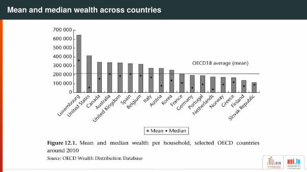
The significant of negative net worth
Net worth is typically the concept of choice for wealth distribution analysis, andNW 6 0 (when debts exceed assets) is a perfectly valid outcome.
In HFCS Wave 1, for example, the fraction of households with non positive net worthreaches
Netherlands 12%Finland 11%Germany 9%
or 14% in the US in LWS/SCF 2010

Immediate consequence
• Many popular inequality measures based on logarithmic or fractional powertransformations are undefined• notably: Atkinson measures, Generalized Entropy measures for α < 2 (incl. Theil,
MLD), the SD of logs
• ... and even percentile ratios or quantile share ratios based on, say, the bottomdecile become undefined or somewhat ‘meaningless’
• Analysts often left with (Generalized) Gini coefficient (or other ‘linear inequality’measures) or the CoV
/⇒ the symptom of a deeper conceptual issue with ‘relative inequality measures’
(Jenkins and Jäntti, 2005)

1. Rethinking ‘maximum inequality’
We first need to rethink what ‘maximum inequality’ is!
• Is inequality maximal when one person has all wealth and everyone else hasnothing (Gini equal to 1)?• If debt is allowed, further ‘regressive transfers’ (from a poor to a rich person) can
take place by further indebting the poor household and enriching the rich household/⇒ No theoretical ‘maximum’ (and the Gini can go beyond 1 when the Lorenz curve
bends below zero)• Justification of ‘renormalisation approaches’ unclear (Chen et al., 1982, Berrebi and
Silber, 1985)
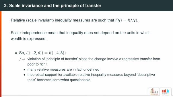
2. Scale invariance and the principle of transfer
Relative (scale invariant) inequality measures are such that I(y) = I(λ y).
Scale independence mean that inequality does not depend on the units in whichwealth is expressed.
• So, I((−2, 4)) = I((−4, 8))/⇒ violation of ‘principle of transfer’ since the change involve a regressive transfer from
poor to rich!• many relative measures are in fact undefined• theoretical support for available relative inequality measures beyond ‘descriptive
tools’ becomes somewhat questionable
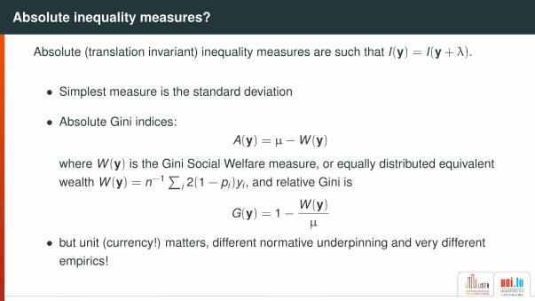
Absolute inequality measures?
Absolute (translation invariant) inequality measures are such that I(y) = I(y + λ).
• Simplest measure is the standard deviation
• Absolute Gini indices:A(y) = µ− W (y)
where W (y) is the Gini Social Welfare measure, or equally distributed equivalentwealth W (y) = n−1∑
i 2(1 − pi)yi , and relative Gini is
G(y) = 1 −W (y)µ
• but unit (currency!) matters, different normative underpinning and very differentempirics!

Absolute and relative Gini coefficients
Relative Gini
ATAT AT
BEBE
BE
CYCY CY
DE DE DE
ES ESES
FI FIFI
FR FRFR
GR GRGR
IT ITIT
LU LULU
MTMT MT
NLNL
NLPT PTPT
SISI
SI
SK SK
SK
.4.5
.6.7
.8va
lue
0 .2 .4 .6 .8 1theta
Absolute Gini
AT
AT
AT
BE
BE
BE
CY
CY
CYDE
DE
DE
ES
ES
ES
FI
FIFI
FR
FRFR
GR
GRGR
IT
IT
IT
LU
LU
LU
MT
MT
MTNL
NLNL
PT
PTPT
SI
SISISK
SK SK020
0000
4000
0060
0000
valu
e
0 .2 .4 .6 .8 1theta

Theme Three
Age, life-cycle accumulation and wealthinequality

Age wealth profiles
UK
02
46
810
1214
Aver
age
net w
orth
(in y
ears
of a
vera
ge a
nnua
l inc
ome)
20 30 40 50 60 70 80 90Age of household head
FR
02
46
810
1214
Aver
age
net w
orth
(in y
ears
of a
vera
ge a
nnua
l inc
ome)
20 30 40 50 60 70 80 90Age of household head
IT
02
46
810
1214
Aver
age
net w
orth
(in y
ears
of a
vera
ge a
nnua
l inc
ome)
20 30 40 50 60 70 80 90Age of household head
US
02
46
810
1214
Aver
age
net w
orth
(in y
ears
of a
vera
ge a
nnua
l inc
ome)
20 30 40 50 60 70 80 90Age of household head
‘Hump shape’ relationshipbetween age and wealth
Peak at 60–65
Remarkably consistentacross countries
How much of wealthinequality is merely due toage mix?
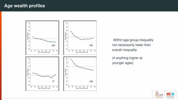
Age wealth profiles
UK
.35
.45
.55
.65
.75
.85
.95
1.05
Gin
i coe
ffici
ent
20 30 40 50 60 70 80 90Age of household head
FR
.35
.45
.55
.65
.75
.85
.95
1.05
Gin
i coe
ffici
ent
20 30 40 50 60 70 80 90Age of household head
IT
.35
.45
.55
.65
.75
.85
.95
1.05
Gin
i coe
ffici
ent
20 30 40 50 60 70 80 90Age of household head
US
.35
.45
.55
.65
.75
.85
.95
1.05
Gin
i coe
ffici
ent
20 30 40 50 60 70 80 90Age of household head
Within age-group inequalitynot necessarily lower thanoverall inequality
(if anything higher atyounger ages)
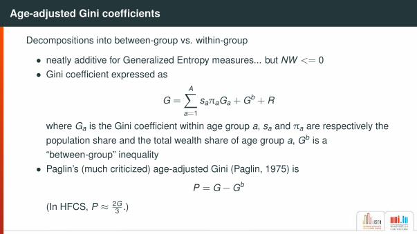
Age-adjusted Gini coefficients
Decompositions into between-group vs. within-group
• neatly additive for Generalized Entropy measures... but NW <= 0• Gini coefficient expressed as
G =
A∑a=1
saπaGa + Gb + R
where Ga is the Gini coefficient within age group a, sa and πa are respectively thepopulation share and the total wealth share of age group a, Gb is a“between-group” inequality• Paglin’s (much criticized) age-adjusted Gini (Paglin, 1975) is
P = G − Gb
(In HFCS, P ≈ 2G3 .)

Age-adjusted Gini coefficients
More general approaches re-express Gini as sum of all pairwise deviations from mean
G =1
2µn2
∑i
∑j
|(wi − µ) − (wj − µ))|
and then use an alternative wealth ‘reference’ (e.g. Almås and Mogstad, 2012)
AG =1
2µn2
∑i
∑j
|(wi − µ(ai)) − (wj − µ(aj))|
Alternative approaches tend to lead to much higher age-adjusted Gini’s than Paglin’s(much closer to unadjusted values)

Theme Four
Inference

Inference with heavy-tailed distributions
Wealth distributions have a much heavier tail than income distributions. Inferenceproblems arising from sparse, extreme data in survey samples discussed in Cowelland Flachaire (2007) and Davidson and Flachaire (2007) are compounded.
• Point estimates are sensitive to extreme data and contamination
• Imprecise estimates even in fairly large samples
• Standard methods for estimation of sampling variance and confidence intervalscalculation perform poorly (both linearization and standard bootstrap methods);e.g. confidence intervals that do not cover the ‘true’ value as per the nominal level
• Non-sampling error: the ‘missing rich’ (see, e.g., Vermeulen, 2016, Kennickell,2019)

Influence functions
SK0
2040
60IF
(w;v
,F)/v
(F)
0 200000 400000 600000 800000Net worth
Gini CoVGE(2)
The influence of extremedata is large, even for SKexample
Especially large for CoV andGE(2)—hardly useable
Semi-parametric estimation for improving inference
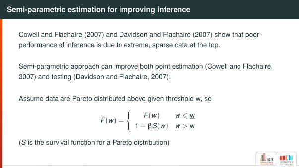
Cowell and Flachaire (2007) and Davidson and Flachaire (2007) show that poorperformance of inference is due to extreme, sparse data at the top.
Semi-parametric approach can improve both point estimation (Cowell and Flachaire,2007) and testing (Davidson and Flachaire, 2007):
Assume data are Pareto distributed above given threshold w, so
F̃ (w) =
{F (w) w 6 w
1 − βS(w) w > w
(S is the survival function for a Pareto distribution)
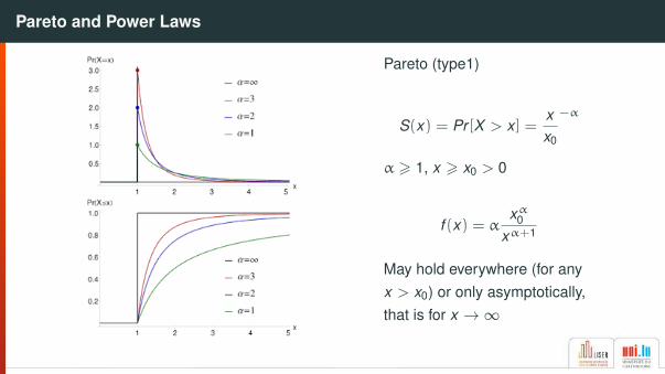
Pareto and Power Laws
Pareto (type1)
S(x) = Pr [X > x ] =xx0
−α
α > 1, x > x0 > 0
f (x) = αxα
0
xα+1
May hold everywhere (for anyx > x0) or only asymptotically,that is for x →∞

Pareto diagram
Plot log(w) against log(1 − F (w)):

A simple, practical approach
1. Estimate α by standard methods from the top k observations (Hill’s index,likelihood formula)• Estimate for alternative k and choose value where α̂ stabilizes• ‘robust’ estimator for α even better, but typically not necessary• NB: k/n may be greater than β
2. Inspect Pareto diagram to select β (or w), e.g., between 0.005 and 0.001,
3. Generic solution (Van Kerm, 2007, Alfons et al., 2013):• discard data wi > w, simulate large number of new data from Pareto distribution,
reweight those draws by β× n / nsim• proceed with estimation as with sample data
(see also Eckerstorfer et al., 2016, Blanchet et al., 2017, Charpentier and Flachaire,2019)

To wrap up

Key messages and challenges
• We know it but, yes, wealth is very unequally distributed: the upper tail spreadsout far away
• Age-wealth profiles are clearly marked ... but within-age-group wealth inequality isnot much smaller than overall inequality
Measuring wealth inequality is not just like income inequality
• (Wealth definition, collection and valuation difficult and crucial!)
• Implication of nature of wealth (negative and not directly ‘consumed’) on standardconcepts and methods need to be appreciated
• Extend ‘toolbox’ to include absolute and age-adjusted measures
• Inference issues are compounded by the heavy tail of the distribution

Some basic accounting identities
• Wealth accumulation (savings and capital gains)
ait+1 = ait(1 + q(i)t) + ∆it + sit
• Income allocation by source and purpose
yit = yLit + yK
it + yTBit = sit + cit
• Capital and labour income (wage times employment)
yLit = w(i)t lit yK
it = r(i)tait
• Net tax-benefit transfer
yTBit = bit − τ
L(i)ty
Lit − τ
L(i)ty
Kit )

References i
References
Alfons, A., Templ, M. and Filzmoser, P. (2013), ‘Robust estimation of economic indicators from surveysamples based on Pareto tail modelling’, Journal of the Royal Statistical Society: Series C (AppliedStatistics) 62(2), 1–16.
Almås, I. and Mogstad, M. (2012), ‘Older or wealthier? The impact of age adjustment on wealthinequality’, Scandinavian Journal of Economics 114(1), 24–54.
Berrebi, Z. M. and Silber, J. (1985), ‘The Gini coefficient and negative income: A comment’, OxfordEconomic Papers 37(3), 525–526.URL: http://www.jstor.org/stable/2663310
Blanchet, T., Fournier, J. and Piketty, T. (2017), Generalized Pareto curves: Theory and applications,WID.world Working Paper 2017/3, World Wealth and Income Database, Paris.
References ii
Charpentier, A. and Flachaire, E. (2019), Pareto models for top incomes, Université Paris1Panthéon-Sorbonne (Post-Print and Working Papers) hal-02145024, HAL.URL: https://ideas.repec.org/p/hal/cesptp/hal-02145024.html
Chauvel, L., Hartung, A., Bar-Haim, E. and Van Kerm, P. (2019), Income and wealth above the median:New measurements and results for Europe and the United States, in K. Decancq and P. Van Kerm,eds, ‘What Drives Inequality?’, Vol. 27 of Research on Economic Inequality, Emerald PublishingLimited, pp. 89–104.
Chen, C.-N., Tsaur, T.-W. and Rhai, T.-S. (1982), ‘The Gini coefficient and negative income’, OxfordEconomic Papers 34(3), 473–478.URL: http://www.jstor.org/stable/2662589
Cowell, F. A. and Flachaire, E. (2007), ‘Income distribution and inequality measurement: The problem ofextreme values’, Journal of Econometrics 141(2), 1044–1072. doi:10.1016/j.jeconom.2007.01.001.

References iii
Cowell, F. A., Nolan, B., Olivera, J. and Van Kerm, P. (2017), Wealth, top incomes, and inequality, inK. Hamilton and C. Hepburn, eds, ‘National Wealth: What is Missing, Why it Matters’, Oxford UniversityPress, Oxford, UK, chapter 8, pp. 175–203.
Cowell, F. A. and Van Kerm, P. (2015), ‘Wealth inequality: A survey’, Journal of Economic Surveys29(4), 671–710.
Davidson, R. and Flachaire, E. (2007), ‘Asymptotic and bootstrap inference for inequality and povertymeasures’, Journal of Econometrics 141(1), 141–166.
Eckerstorfer, P., Halak, J., Kapeller, J., Schütz, B., Springholz, F. and Rafael, W. (2016), ‘Correcting for themissing rich: An application to wealth survey data’, Review of Income and Wealth 62(4), 605–627.
Jenkins, S. P. and Jäntti, M. (2005), Methods for summarizing and comparing wealth distributions, ISERWorking Paper 2005-05, Institute for Social and Economic Research, University of Essex, Colchester,UK. http://www.iser.essex.ac.uk/pubs/workpaps/pdf/2005-05.pdf, forthcoming inConstruction and Usage of Comparable Microdata on Household Wealth: The Luxembourg WealthStudy, Banca d’Italia, Roma.

References iv
Kennickell, A. B. (2019), ‘The tail that wags: differences in effective right tail coverage and estimates ofwealth inequality’, The Journal of Economic Inequality 17(4), 443–459.
Kuhn, M. and Ríos-Rull, J.-V. (2016), ‘2013 update on the U.S. earnings, income, and wealth distributionalfacts: A view from macroeconomics’, Federal Reserve Bank of Minneapolis Quarterly Review37(1), 1–73.
Paglin, M. (1975), ‘The measurement and trend of inequality: A basic revision’, The American EconomicReview 65(4), 598–609.
Van Kerm, P. (2007), Extreme incomes and the estimation of poverty and inequality indicators fromEU-SILC, IRISS Working Paper 2007-01, CEPS/INSTEAD, Differdange, Luxembourg.
Vermeulen, P. (2016), ‘Estimating the top tail of the wealth distribution’, American Economic Review:Papers & Proceedings 106(5), 646–650.