Wealth Accumulation and Factors Accounting for Success

Anan Pawasutipaisit, University of Chicago

Robert M. Townsend∗, Massachusetts Institute of Technology

February, 2010

JEL classification: D31, D24, D92

Keywords: Wealth accumulation, Wealth inequality, Return on assets,

Heterogeneity, Persistence

Abstract

We use detailed income, balance sheet, and cash flow statements constructed for households

in a long monthly panel in an emerging market economy, and some recent contributions in

economic theory, to document and better understand the factors underlying success in achieving

upward mobility in the distribution of net worth. Wealth inequality is decreasing over time, and

many households work their way out of poverty and lower wealth over the seven year period.

The accounts establish that, mechanically, this is largely due to savings rather than incoming

gifts and remittances. In turn, the growth of net worth can be decomposed household by

household into the savings rate and how productively that savings is used, the return on assets

(ROA). The latter plays the larger role. ROA is, in turn, positively correlated with higher

education of household members, younger age of the head, and with a higher debt/asset ratio

and lower initial wealth, so it seems from cross-sections that the financial system is imperfectly

channeling resources to productive and poor households. Household fixed effects account for

the larger part of ROA, and this success is largely persistent, undercutting the story that

successful entrepreneurs are those that simply get lucky. Persistence does vary across households,

and in at least one province with much change and increasing opportunities, ROA changes as

households move over time to higher-return occupations. But for those households with high and

persistent ROA, the savings rate is higher, consistent with some micro founded macro models

∗Corresponding address: Department of Economics, 50 Memorial Drive; Room E52-252c, Cambridge, Massa-

chusetts 02142 Tel: (617) 452-3722. Email: rtownsen@mit.edu

1

with imperfect credit markets. Indeed, high ROA households save by investing in their own

enterprises and adopt consistent financial strategies for smoothing fluctuations. More generally

growth of wealth, savings levels and/or rates are correlated with TFP and the household fixed

effects that are the larger part of ROA.

1 Introduction

We use detailed income and balance sheet statements constructed for households in a long monthly

panel in an emerging market economy to document and better understand the factors underlying

success in achieving upward mobility in the distribution of net worth. The overall growth rate of

wealth when accounting for inflation is only a modest 0.3% per year and the wealth distribution is

highly skewed, with the relatively rich holding a third of net worth and the bottom half holding less

than 10%. But the growth rate of wealth over time is sharply decreasing in initial wealth levels,

that is, the relatively poor grow much faster than the rich, at 22% per year vs. 0.09% per year.

Further decompositions show that overall inequality comes down substantially as households either

transit upwardly over time across initial wealth quartiles or as wealth increases on average for the

lower quartiles, so that the gaps across the quartiles narrow. Geographic location and occupation

contribute less than what we might have expected to this story. There is initially increasing wealth

inequality across regions for some occupations, increasing for fish/shrimp and cultivation overall and

for labor and business initially. But the larger force, about 60%, is the reduction of inequality within

the residual category.

Some of the more successful households experience large increases in their relative position in the

wealth distribution, while others fall down. Approximately 7% of households in the survey stayed at

the same relative position, 43% increased their position, and almost 50% have a negative change in

position. The standard deviation of relative position change is 14 points, so again there is substantial

mobility within the distribution.

The constructed accounts also allow an exact decomposition of these changes into net savings

and incoming gifts/remittances. Savings accounts for 81% of the change, and, roughly, gifts decrease

as initial wealth quartiles increase. The rich actually give some money away, for example. But for

the second quartile of initial wealth, incoming gifts play a role equal to savings, even more so for

households running businesses (as enterprises made losses in early years).

Another decomposition allows us to separate the increase in net worth into the role played by

2

the savings rate versus how effectively those savings are used, that is, the return on assets (ROA).

Growth of net worth is positively and significantly correlated with savings rates but less so than

the high and consistently significant correlation of the growth of net worth with ROA, across the

board. In this sense, successful households with high growth of net worth are the households who

are productive — who utilize their existing assets to produce high per unit income streams.

In turn we can search for significant covariates of ROA. There is a positive correlation of high

ROA with low initial net worth (i.e., the poor are especially productive), a higher education of the

head or among household members (especially for those running businesses), a younger age of the

head of the household, and a high debt/asset ratio (as we comment on below).

In the robustness checks we control for labor hours and, related, impute a wage cost to self-

employment. We also correct for measurement error in initial assets and, in exploring covariates,

use IV rather than OLS regressions. We also delete poor wage earning households with few assets.

Results are robust to these specifications.

But by far the largest single factor in a decomposition of variance are household specific fixed

effects. Related, there is considerable persistence. Households successful over the first half of the

sample are very likely to be successful over the second, indicating that luck per se is not a likely

explanation for this success. Auto-correlation numbers range from 0.15 to 0.83. In one fast-growing

province in the poorer Northeast, persistence is much lower, and there is strong evidence that house-

holds are moving out of lower ROA occupations and into higher ones, as the local economy presents

opportunities. Variability in household size also undercuts persistence, highlighting the importance

of a successful individual rather than a successful household per se. Northeastern households expe-

rience more volatility in membership.

As noted in passing above, there is some borrowing, and indeed, high ROA households have

higher debt/asset ratios. It thus appears that the financial system does manage to some degree to

extend credit to the poor with high returns. Indeed, using more structure for production functions,

and using instruments suggested by Olley and Pakes (1996), and Levinsohn and Petrin (2003), we

find that high marginal product of capital (MPK) households are likely to borrow more relative

both to their wealth and to others. However, there is still a divergence between estimated MPK and

average interest rates, so in that sense some households are constrained (a related distortion, others

utilize their own wealth at a low return rather than allowing it to be intermediated). Further, we

allow interest rates to vary across households as measured in the survey data, as if there were a wedge

or distortion from the average, as in Hsieh and Klenow (2009), Restuccia and Rogerson (2008), and

3

Fernandes and Pakes (2008). Re-estimated TFP is no longer correlated with the debt/asset ratio,

as if we had now correctly accounted in this way for those credit market distortions, or other things.

The dynamics coming from the panel are revealing about the distortions which are harder to

rationalize. Consistent with a literature on growth with financial frictions, we find, using monthly

data, that households with high and persistent ROA are households that tend to save more. This is

consistent with the models of Buera (2008) that poor households can save their way out of constraints,

say to eventually enter high return businesses, or expand existing businesses. However, this result

is not robust to annual data. In the model of Moll (2009) and Banejeree and Moll (2009) persistent

ROA should increase the growth of net worth as households save their way out of constraints. Overall

however savings levels and rates and growth of wealth are all correlated with the level of ROA, the

household fixed parts of ROA, and measured TFP.

As further evidence of constraints, high ROA households tend to save by investing, that is,

they accumulate physical assets. The top quartile of ROA households invest in their own enterprise

activities, but this is not the case for the middle and lower ROA groups. Instead, for many, increases

in net worth are accomplished with increases in financial assets or cash saving. Related, relative

to others in the cross-section, high ROA households are less likely to use capital assets to smooth

consumption. Instead, they use consumption to finance investment deficits. High ROA households

are more actively involved in financial markets month by month, in the sense of using formal savings

accounts and sources of borrowing, and engage less in informal markets, i.e., receiving fewer gifts. But

high ROA households do use cash more than the low ROA households, as well. Indeed, relatively

high ROA households surprisingly do seem to seek financial autarky over time; in the long run

reducing their debt, reducing the amount of gifts they receive, and increasing the amount in formal

savings accounts. This even though they retain a relatively high ROA.

As ROA is a widely accepted indicator of success in corporate accounting, but less so in economic

theory, we also estimate total factor productivity (TFP) as was anticipated earlier. We find that it is

correlated with ROA and in turn with candidate covariates, but less than before. The data are also

adjusted for aggregate risk, consistent with the perfect markets, capital asset pricing model at the

village level, utilizing the work of Samphantharak and Townsend (2009). We find a correlation of

risk-adjusted returns with ROA, as a measure of individual talent, and a correlation of risk-adjusted

returns with growth of net worth. But overall results are weaker, for example, high risk-adjusted

return households do not invest more in their own enterprises. This suggests again that the capital

markets are not perfect in these data, though there remains some consumption anomalies which we

4

discuss at the end.

This paper is organized as follows. Section 2 describes the data, starting from a macro-level

perspective as background and moving to the micro-level of selected areas from which we have

detailed information on assets, liabilities, wealth, income, consumption, investment, and financial

transactions. Section 2 also describes the wealth distribution and its decomposition. Section 3

decomposes growth of net worth into productivity and saving rates, and uses correlation analysis to

show their relative importance to the growth of net worth. Section 4 uses regression analysis to find

out what factors are associated with success as measured by a high rate of return on assets. Section

5 shows that ROA has considerable persistence, indicating that luck per se is not systematically

related to success. Section 6 shows the predictive power of ROA on physical assets accumulation.

Section 7 studies the financial strategies that high ROA households use and related imperfections in

credit markets. Section 8 provides a short story of a selected successful household, as a case study,

to complement the overall statistical analysis, and section 9 concludes.

2 Data

This paper uses data from the Townsend Thai monthly survey,1 an ongoing panel of households

being collected since 1998. The survey is conducted in 4 provinces (or changwat in Thai), the semi-

urban changwats of Chachoengsao and Lopburi in the Central region and the more rural Buriram

and Sisaket in the poorer Northeast region (see the map in Figure 1 below). This paper studies

the balanced panel of 531 households that are interviewed on a monthly basis, dating from January,

1999, to December, 2005 (seven years).2 In each province one tambon (county) and four villages

per tambon were selected at random from a larger 1997 survey. With only 16 villages overall, this

naturally raises some questions about the representativeness of the sample. So we also report here

on the background from secondary sources, which is largely consistent.

For comparability over time we put variables into real terms with 2005 as the benchmark for

both data sets.1See further details of sampling design of this survey from Binford, Lee and Townsend (2004).2Attrition is typically one of the most serious problems involving panel data, and this survey is no exceptioin. For

those households with incomplete panel, the two main reasons are temporary migration (42%) and household member

with relevant information is not available (26%). However, 60% of the incomplete panel consist of wage earner, and

below we drop all wage earner from some of the analysis for other reasons.

5

2.1 Background at Macro-Provincial Level

Figure 1 is from the Thai Socio-Economic Survey, a nationally representative household survey

conducted by the National Statistics Office of Thailand. Unfortunately there is no time series

of wealth data in this survey. So we pick per capita net income to represent levels and what has

happened over the past eighteen years. As is evident from the right panel, with all provinces depicted

and the sample provinces highlighted, Buriram and Sisaket in the Northeast are among the poorest

provinces in the entire nation. Chachoengsao and Lopburi are in the upper end of the distribution,

though not the very highest (we do not have data in the SES for Chachoengsao over all years).

However, it is also apparent that Lopburi is growing relatively faster.

Concentrating on the period of our own study here, the left panel is the ratio of per capita

income from 1996 to 2006, relative to 1996. Here one can see the heterogeneity in growth, with high

growth concentrated in the central region, but also in some parts of the Northeast and the South.

Again, Lopburi stands out as growing relatively faster. Buriram is also doing quite well over this

time frame. Chachoengsao and Sisaket are in the lower quartile. Evidently Sisaket is poor and tends

to stay poor. Chachoengsao is relatively rich, but not growing much.

[Figure 1 here]

2.2 Poverty Reduction

Over the seven year time frame of the survey, many households work their way out of poverty. We

use two measures of the poverty line here. First is the Thai official number for each province, which

we can compare to either per capita income or to consumption. Second is a standard benchmark

consumption of $2.16 a day at 1993 PPP. These two poverty lines generate some differences in the

measure of poverty.

By location, there are many more poor in the Northeast. As is evident in Figure 2, income

(especially for farmers) is erratic: monthly income displays nontrivial fluctuations. But we can still

look at trends, that is, the overall picture and whether the number of poor people is decreasing over

time by occupation, and by location (not shown). Using these high frequency monthly data, the

headcount ratio fluctuates with a clear cycle in the Northeast. Poverty drops at harvest, the time

when many households receive income from cultivation. This figure also indicates that the fraction

of poor households in business is declining substantially. There are gains for livestock and modest

6

gains for labor. But in terms of change, the biggest gains are in Buriram (not shown).

[Figure 2 here]

Using consumption numbers, there are a lower numbers of poor than by using the income measure,

especially in the Central region. By location, the biggest gains are still in Buriram. By occupation,

labor and business escape poverty relatively fast.

2.3 Measurement and the Accounting Framework

The Townsend Thai survey interviews households on a monthly basis (and bi-weekly for food con-

sumption). Given that households are typically a production as well as a consumption unit, we treat

households as corporate firms, as described in Samphantharak and Townsend (2009), and impose

onto each of the transactions of the monthly data a financial accounting framework.

Each flow transaction is classified as being associated with production activities, consumption

and expenditure, and financing and saving, for instance. This allows us to construct the balance

sheet and the income statement of each household. Then we add the flow variables into the previous

period stocks to get the current values of stock variables for each month for each household. The

updated stock at the end of each month corresponds to the items in the balance sheet. Wealth

or net worth in particular is equal to total assets minus total liabilities. It must also be equal to

contributed capital plus cumulative savings.

We then derive the statement of cash flow from the constructed balance sheet and income state-

ment and double check accounting identities between the balance sheet, the income statement and

the statement of cash flow of each household, month-by-month, to make sure that the accounting

framework is correctly imposed.

As the survey was not initially designed for this purpose, we sometimes have to make assumptions

and refine the value of a transaction before we enter it into the appropriate line item. For instance,

when household members migrate to work somewhere else, we do ask them when they returned how

much they earned while they were away. If this is labor earnings, then this will show up as labor

income. But they often send home remittances while they are away (thus treated as non-household

member while away), and if we do not adjust for this, we may be double-counting, as otherwise we

have both gift-in and labor income. In turn, we would overestimate the wealth of the household.

Another example is cash holding. We do not ask for the amount of cash in hand, as this question

might be sensitive and affect answers to other questions or even participation in the survey, but for

7

any transactions we do ask whether it is done in cash, kind or on credit, so in principle we know

the magnitude of all cash transactions. We then as a first step in an algorithm specify that initial

cash is zero and then subsequently keep track of the changes. If they spend too much, cash balances

will become negative. We reset the initial balance to a higher number such that in the data they

never run out of cash. This algorithm, therefore, gives us a lower bound on cash holding. Sometimes

discrepancies remain, and then we have to check manually, household by household, as the answers

from a household can be more complicated than the existing code can accommodate. Additional

difficulties are due to recall error, change in household composition, and appreciation in value of

assets. Regarding recall error, a household may simply forget to tell us their relevant transaction

at some point, but later with a myriad of additional questions we find out about that transaction.

Then we have to go back and fix it. For change in household composition, an existing member might

leave the household and a new member might move in, and as they often take some assets with them

or bring new assets in, we have to take appropriately care. For value appreciation, especially land,

it is possible that land was cheap in the past when the household started owning it, but that price

went up by the time the household sold it. We take care of this by having capital gains items in the

income statement and appropriately adjusting this appreciation in the balance sheet.

Though we believe that the accounting framework gives us a more accurate measurement than

otherwise, measurement errors in the survey data cannot be avoided. We will keep the possibility of

measurement errors in mind and revisit this in the appropriate sections below.

Lastly, there is the distinction between nominal and real terms. The accounting framework is

constructed based on observed transactions, hence nominal units. We lose some of the identities

when we convert the data to real terms. For most of the analysis in the paper we use real units for

comparability over time. However, when we must rely on an accounting identity, we use nominal

terms.3

2.4 Wealth Distribution in the Townsend Thai Monthly Survey

Table 1 reports the distribution of average wealth, by location and overall in 1999, in nominal

baht value (the exchange rate was 37.81 baht for $1 in 1999, and on average 41.03 baht per $1 for

1999-2005). The median wealth in 1999 was about $20,000.

[Table 1 here]

3See further details of how to construct the account from the survey data from Pawasutipaisit, Paweenawat,

Samphantharak and Townsend (2007).

8

By region, the top two provinces in the Central region are evidently wealthier than the bottom

two in the Northeast. Within regions, Chachoengsao is wealthier than Lopburi, and Buriram is

wealthier than Sisaket. These are consistent with the background data from the SES, even though

income per capita was used there.4

There are five primary sources of income for households in the survey: cultivation, livestock,

fish/shrimp, business and labor. Households in the survey typically have income from multiple

sources, and one can label as the primary occupation the activity that generates the highest net

income over some period. Table 2 shows the number of households in each occupation where we

use the activity that generates highest net income over seven years (here by construction, these

households do not "change" occupations/bins over time). As is evident, shrimp is associated with

Chachoengsao, livestock with Lopburi.

[Table 2 here]

Table 3 reports the distribution of average wealth, by occupation, in 1999. By medians, fish/shrimp,

livestock and business households are wealthier than those in cultivation.5 Labor households appear

to be the least wealthy, both in mean and median.

[Table 3 here]

We now focus on the distribution of wealth.6 Table 4 shows that households in the top 1% of the

wealth distribution hold around one-third of the total wealth in the survey, the top 5% hold about

half of the total wealth. Half of the households in the survey own less than 10%. These numbers may

understate wealth inequality if the rich are undersampled. These observations as given are similar

to findings from developed countries like the United States, Britain (see Atkinson (1971), Kennickell

(2003), Piketty and Saez (2003)).7

[Table 4 here]

4The minimum wealth in Sisaket in particular is negative, there are 2 households that are excessively indebted in

1999, even if they liquidate all their assets, they would not be able to pay back all their debts.5The highest net worth household is one with cultivation, but that is an exception.6Because households in this survey are selected by random sampling, and the survey is not explicitly designed to

measure the distribution of wealth, therefore the actual wealth distribution might be worse than what we report here

if the rich are undersampled.7The degree of wealth inequality varys across location, however, it is highest in Chachoengsao while lower in other

provinces. The top 1% in Lopburi own less than 13% while the top 1% in Sisaket own less than 18% of the total

wealth in their province.

9

Though Table 4 shows the overall picture of wealth inequality, it does not keep households in the

same group over time. Because we have panel data, we can track wealth dynamics at the household

level. Using all observations (household-years), with groups defined from the distribution of average

wealth in year 1999, we track the same group over time.

[Table 5 here]

Table 5 indicates that wealth share is rising for many groups but, especially for the initially poor.

An observation common to all provinces is that the bottom half has a rising share.

By this standard, wealth inequality is thus going down over time. Other well known measures

of inequality give similar reductions. For instance, the aggregate level of wealth inequality dropped

from 0.71 in 1999 to 0.67 in 2005 if we use the Gini coefficient, and inequality went down from 1.26

in 1999 to 1.10 in 2005 if we use the Theil-T index.

2.5 Average Growth of Wealth by Initial Quartile, Location and Occu-

pation

Table 6 documents a salient feature, that growth is decreasing in initial wealth. Every quartile has

positive growth, but the magnitude is indeed remarkable for the poorest group, about 22% per year.

[Table 6 here]

To see where this movement comes from, Table 7 reports the growth of selected assets in household

balance sheet. Land is typically the largest component in household portfolio but it is not the prime

mover of wealth. The growth of household assets is decreasing in initial wealth, and though other

types of fixed assets are not strictly monotone decreasing in initial wealth more upward movement

comes from the bottom 50%. Growth of inventory is also large and decreasing in initial wealth,

although inventory is not a big component of total assets. For financial assets, growth of deposits

in financial institutions is also decreasing in initial wealth, and the growth of cash largely shares

the same pattern, highest for the least wealthiest group and lowest for the wealthiest group, though

mixed in the middle.

[Table 7 here]

The annual percentage increase in net worth by location is presented in Table 8. On average,

total growth rate is about 0.3% per year, but this varies. On average, Lopburi has the highest

growth rate (1.7%). Buriram has the lowest growth due to negative initial growth during the first

10

three years, although it reaches the highest number in the Table in 2003-04 at 6.8%. Chachoengsao,

in contrast, is slowing down and Sisaket is closest to 0 and does not change much compared to the

others. Much of this is consistent with the national background presented earlier.

[Table 8 here]

The annual percentage increase in net worth by occupation is presented in Table 9. On average,

households with livestock have the highest growth rate (2.2%) and households with business the

second highest (1.5%). In contrast, cultivation and fish/shrimp households have negative growth

where the lowest growth is at fish/shrimp (-0.58%). Labor has positive growth (1.28%) but is lower

than livestock and business. All occupations experience negative growth in some periods.

[Table 9 here]

2.6 Decomposition of Wealth Inequality Change by Initial Quartile or

Decile

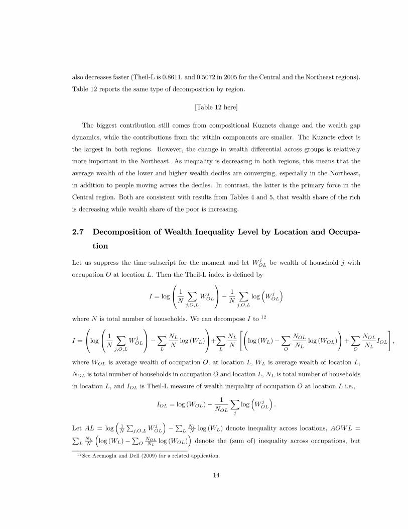
We can also look at entire distributions of wealth. Figure 3 shows estimates of the kernel densities of

wealth distributions (in log scale) when we classify households into four groups, by initial quartile,

and follow each group over time8. The wealth distribution of the poorest group and the second

poorest group shift toward the right, and for the second group it has a wider support. The wealth

distribution of the relatively wealthy group (lower left panel) also become wider. The wealth distri-

bution of richest group (lower right panel) shifts slightly toward the right, but this is not noticeable

from the picture.

[Figure 3 here]

One question is how much of the reduction in wealth inequality is due to the fact that poor

households grow faster, as opposed to other forces. One well known and widely used measure

of inequality is the Theil-L index, which is additively decomposable. Let W j,gt be the wealth of

household j which belongs to group g at time t, and Nt be total number of household at time t.

Then the Theil-L index is defined by

It = log

⎛⎝ 1

Nt

Xj,g

W j,gt

⎞⎠− 1

Nt

Xj,g

log³W j,g

t

´.

8 It might seem that the distribution of initial wealth would have four humps when we pull all groups together. But

this is only an artifact of the four separate kernel estimations. If the four histograms of initial wealth were plotted

and presented in one column, it would be obvious that they are non-overlapping across the four panels.

11

Also let

Ngt = total number of households in group g at time t

W gt =

1

Ngt

Xj

W j,gt

Igt = log (W gt )−

1

Ngt

Xj

log³W j,g

t

´.

Then inequality can be decomposed to a within (WIt) and across (AIt) component

It = AIt +WIt

AIt = log

⎛⎝ 1

Nt

Xj,g

W j,gt

⎞⎠−Xg

Ngt

Ntlog (W g

t )

WIt =Xg

Ngt

NtIgt .

Thus total change inequality must come from changes in each component:

∆I = ∆AI +∆WI.

To simplify the notation, let Wt be an aggregate mean of wealth at time t, pgt be the population

share of subgroup g at time t. Then ∆WI and ∆AI each can be further decomposed into two

subcomponents, 9

∆AI =Xg

µpgW g

W− pg

¶∆ logW g +

Xg

µW g

W− log W

g

W

¶∆pg

∆WI =Xg

pg∆Ig +Xg

Ig∆pg

where ∆ and the overbar denote the time difference operator and the time average operator, respec-

tively.

Each subcomponent has its own interpretation:P

g pg∆Ig is intragroup inequality dynamics or

change in inequality within group,P

g Ig∆pg is composition dynamics through shifts across group

with different degrees of inequality,P

g

³pgWg

W − pg´∆ logW g is wealth-gap dynamics or change in

wealth differential across group, andP

g

³Wg

W − log Wg

W

´∆pg is composition dynamics in changes in

AI. The latter is the Kuznets effect, i.e., shifts by the poor into higher quartiles.

9See Mookherjee and Shorrocks (1982) where ∆WI is exact decomposition while ∆AI is approximate decomposi-

tion.

12

If we use the quartile of the wealth distribution in 1999 to define group then pg1999 = 1/4 for all

g, but again we allow people to move across groups over time, and also the number of households in

each group may vary overtime. Some households with increasing wealth may move up, while those

with decreasing wealth may fall down. Although the boundaries of each cell are fixed over time,

many households move in and out of the cells. The transition matrix from 1999 to 2005 where group

is initial quartile on the left, and by initial decile for comparison on the right, are each reported in

Table 1010.

[Table 10 here]

By quartile, about 20% of households move up and 8% of households fall down. There seems to

be a considerable amount of persistence over time, as almost 72% stay in the same group. However,

by deciles there is more mobility, as 37% of households move up, 21% of households fall down and

only 41% stay in the same group.

[Table 11 here]

Table 11 for deciles reports the percentage of the contribution of each subcomponent to the total

reduction in wealth inequality, year by year and overall from beginning to end. The biggest contri-

bution comes from compositional Kuznets change and the wealth gap dynamics. The contributions

from the two within components are smaller and sometimes negligible.

For the whole period of 1999-2005, the last row indicates that the decrease in wealth inequality

is due to a compositional change, and to convergence in the wealth differential across groups, that

is, 51% and 49% of the reduction in wealth inequality are due to these two components, respectively.

Note that the former is the source of inequality dynamics which Kuznets emphasized, though it was

income that he had in mind, while the latter indicates the convergence in wealth across groups.11

The last two columns indicate that overall within group inequality and a composition effect

can be negative. For example, in the last overall row, the composition effect goes in the opposite

direction from overall inequality, i.e., there are shifts into higher inequality groups.

By region, wealth inequality in both regions is decreasing. The Central region has much higher

inequality (Theil-L is 1.1019 in 1999) than the Northeast (Theil-L is 0.6098 in 1999), but inequality

10The number in each cell is the number of households. One can convert these to fractions (probabilities as in the

conventional transition matrix) by dividing it by sum of the number in each cell across column for each row.11Using quartiles yields similar results but the orders of magnitude are lower because we have fewer bins, i.e.,

the decrease in wealth inequality for the whole period 1999-2005 is due to a compositional change (44.67%), and

to convergence of the wealth differential across groups (39.87%). The two within components account for the rest

(15.46%).

13

also decreases faster (Theil-L is 0.8611, and 0.5072 in 2005 for the Central and the Northeast regions).

Table 12 reports the same type of decomposition by region.

[Table 12 here]

The biggest contribution still comes from compositional Kuznets change and the wealth gap

dynamics, while the contributions from the within components are smaller. The Kuznets effect is

the largest in both regions. However, the change in wealth differential across groups is relatively

more important in the Northeast. As inequality is decreasing in both regions, this means that the

average wealth of the lower and higher wealth deciles are converging, especially in the Northeast,

in addition to people moving across the deciles. In contrast, the latter is the primary force in the

Central region. Both are consistent with results from Tables 4 and 5, that wealth share of the rich

is decreasing while wealth share of the poor is increasing.

2.7 Decomposition of Wealth Inequality Level by Location and Occupa-

tion

Let us suppress the time subscript for the moment and let W jOL be wealth of household j with

occupation O at location L. Then the Theil-L index is defined by

I = log

⎛⎝ 1

N

Xj,O,L

W jOL

⎞⎠− 1

N

Xj,O,L

log³W j

OL

´where N is total number of households. We can decompose I to 12

I =

⎛⎝log⎛⎝ 1

N

Xj,O,L

W jOL

⎞⎠−XL

NL

Nlog (WL)

⎞⎠+XL

NL

N

"Ãlog (WL)−

XO

NOL

NLlog (WOL)

!+XO

NOL

NLIOL

#,

where WOL is average wealth of occupation O, at location L, WL is average wealth of location L,

NOL is total number of households in occupation O and location L, NL is total number of households

in location L, and IOL is Theil-L measure of wealth inequality of occupation O at location L i.e.,

IOL = log (WOL)−1

NOL

Xj

log³W j

OL

´.

Let AL = log³1N

Pj,O,LW

jOL

´−P

LNL

N log (WL) denote inequality across locations, AOWL =PLNL

N

³log (WL)−

PO

NOL

NLlog (WOL)

´denote the (sum of) inequality across occupations, but

12See Acemoglu and Dell (2009) for a related application.

14

within location, and WOWL =P

LNL

N

³PO

NOL

NLIOL

´denote the (sum of) inequality within occu-

pations, within locations.

[Figure 4 here]

[Table 13 here]

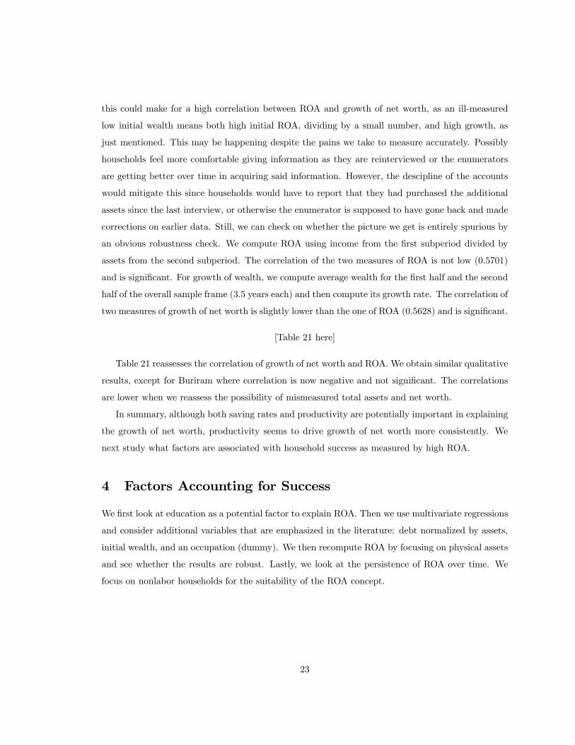
Overall, the within location occupation category is the largest. The second largest is across

location, and the across occupation within location effect is the smallest. These are plotted in

Figure 4 but on different scales.

In terms of changes, Table 13 and Figure 4 confirm that overall inequality I (Theil-L) is going

down over time, where the residual WOWL is the biggest component among the three.

Wealth inequality across locations AL has an inverted U-shape, i.e., increasing until 2002 and

decreasing after that, and wealth inequality across occupation but within location has a decreasing

trend.

Within occupation/location, inequality is not decreasing everywhere. For example, business al-

most everywhere has an increasing trend (except Sisaket). Still, cultivation and labor have decreasing

inequality everywhere and the biggest drop is in cultivation in Chachoengsao. Since most households

have labor and cultivation as a primary occupation, these together drive down the aggregate value

of this component, WOWL.

We can also reverse the order in decomposition and then look at inequality across occupations,

and inequality within occupations but across locations:

I =

⎛⎝log⎛⎝ 1

N

Xj,O,L

W jOL

⎞⎠−XO

NO

Nlog (WO)

⎞⎠+XO

NO

N

"Ãlog (WO)−

XL

NOL

NOlog (WOL)

!+XL

NOL

NOIOL

#,

whereWO is average wealth of households with occupation O, and NO is total number of households

with occupation O.

LetAO = log³1N

Pj,O,LW

jOL

´−P

ONO

N log (WO) denote inequality across occupations, ALWO =PO

NO

N

³log (WO)−

PLNOL

NOlog (WOL)

´denote the (sum of) inequality across location, but within

occupation, and WLWO =P

ONO

N

PLNOL

NOIOL the same as before, i.e., residual is a residual. The

following Table 14 and Figure 5 are the decompositions of their Theil-L indices by occupation and

location.

[Table 14 here]

15

[Figure 5 here]

Of course, the within occupation and within location number is the same as before and the

largest. Inequality across occupations is the second largest, but the difference between the first and

second rows is smaller than before. In terms of changes, Table 14 shows that ALWO has an inverted

U-shape. Inequality across locations is increasing as before, up to about 2002, now controlling in a

sense for occupation. We also see that inequality across occupations, not controlling for location, is

now slightly increasing at the beginning, i.e., going against the overall trend. These are plotted in

Figure 5 but on different scales.13

2.8 Decomposition of Growth of Net Worth: The Mechanics

We return to the financial accounts (in nominal terms) to begin to get at the mechanics of the

change in net worth for each household. The change in net worth of each household must come from

savings and net gifts received. That is, let ∆W it =W i

t −W it−1 be the change in net worth at time t

of household i, Sit and Git be savings (saved if positive or dissaved) and gifts (received if positive or

given) at time t of household i. Hence:

W it =W i

t−1 + Sit +Git.

More generally, wealth or net worth at time t can also be expressed as initial wealth W i0 plus

accumulated savings and net gifts received up to time t:

W it =W i

0 +tX

j=1

¡Sij +Gi

j

¢.

We may ask which component is the larger part of the rate of total wealth accumulation in this

economy in the aggregate:

1Ng

PNg

i=1

¡W i

t −W i0

¢1Ng

PNg

i=1Wi0

=1Ng

PNg

i=1

Ptj=1 S

ij

1Ng

PNg

i=1Wi0

+1Ng

PNg

i=1

Ptj=1G

ij

1Ng

PNg

i=1Wi0

, (1)

13Looking at the subcomponents of ALWO by occupation makes it clearer why both AL and ALWO have inverted

U shapes, due to business and labor. But ALWO is increasing for cultivation, fish/shrimp, while decreasing for

livestock. That is, the premia across location, the wealth differential according to location, is going up consistently

for cultivation and fish/shrimp, increasing until 2002 and decreasing after that for business and labor while the one

for livestock is going down consistently. As we add them up, the combination of these forces together produce the

picture of ALWO as inverted U-shape as seen in Figure 5, which is also similar to the picture of AL in Figure 4.

16

where Ng is the total number of households in a group g. Thus, the left-hand side variable measures

the overall aggregate growth rate of the net worth of group g.

We can now decompose the aggregate growth rate into a weighted sum of growth from these

subgroups by group g. Using the notation defined as before, let Wt be aggregate mean of wealth

at time t, and let pgt and W gt be population share and mean of subgroup g, respectively. Then the

aggregate mean change in levels can be decomposed into two parts, due to a change in the mean of

subgroups and a change in population shares:

∆W =GXg=1

pg∆W g +GXg=1

W g∆pg,

where again ∆ and the overbar denote the time difference operator and the time average operator,

respectively. The first term captures intragroup growth, while the second term captures growth due

to compositional change in population. But as a subgroup is defined by the distribution of initial

wealth, e.g., quartiles, and we follow households in the same group over time, then pgt will not change

over time so,

∆W =GXg=1

pg∆W g.

Dividing both sides by W0 to compute the overall aggregate growth rate, the latter is related to

growth rate of the subgroup by:

1N

PNi=1

¡W i

t −W i0

¢1N

PNi=1W

i0

=GXg=1

pg1Ng

PNg

i=1

¡W i

t −W i0

¢1Ng

PNg

i=1Wi0

1Ng

PNg

i=1Wi0

1N

PNi=1W

i0

. (2)

Substituting (1) into (2), we can thus decompose the overall aggregate growth of each group into

three components: wealth weight in the total, savings, and gifts.

1N

PNi=1

¡W i

t −W i0

¢1N

PNi=1W

i0

=GXg=1

pg

Ã1Ng

PNg

i=1

Ptj=1 S

ij

1Ng

PNg

i=1Wi0

+1Ng

PNg

i=1

Ptj=1G

ij

1Ng

PNg

i=1Wi0

!1Ng

PNg

i=1Wi0

1N

PNi=1W

i0

(3)

Each element in (3) is presented in Table 15 where again group g refers to initial quartiles and takes

t to be the terminal period that the data is available. Table 15 reports overall growth rate, savings

and gift components (annualized value), and wealth weight that can account for the growth of each

group.

[Table 15 here]

The growth of wealth is decreasing in initial wealth, as noted earlier across the quartiles. The

savings component is the one that accounts for most of the growth rate. Largely, the contribution

17

of gifts decreases as wealth increases, except for the second quartile where both savings and gift

components are roughly the same. The wealthiest group has a negative gift component, that is, they

give more than they receive on average, and that brings down its growth of net worth. Even though

the least wealthy group has a growth rate of over 25%, its fraction of initial mean wealth is only

6%, while the wealthiest group, with its 1.5% in growth rate, has an initial mean out of aggregate of

over three-fold. Thus, the overall growth of the (nominal) net worth of the economy is about 2.7%

per year, and 81% of this growth is accounted for by the savings component.

Although the wealth of all groups is growing, the process not smooth, especially at high temporal

frequencies. If we look at the monthly aggregate change in the net worth of each group (from January,

1999, to December, 2005), this can be decomposed again into aggregate savings and gifts of that

quartile group g :

1

Ng

NgXi=1

∆W it =

1

Ng

NgXi=1

¡Sit +Gi

t

¢.

We can see from Figure 6 that all groups experience negative growth at some points.

[Figure 6 here]

Another way to look at the role of savings and gifts in the change in net worth is to use a variance

decomposition. By the accounting identity, again, change in net worth of each household must be

equal to savings plus net gifts received. This identity can be translated to a statistical relationship:

1 =cov

¡∆NW i, Si

¢var (∆NW i)

+cov

¡∆NW i, Gi

¢var (∆NW i)

for all i,

that is, normalized wealth change can be accounted by the co-movement of wealth change with saving

and the same with net gifts. By this metric, the variation in wealth change for most households

is, again, better explained by variation in savings rather than gifts, as the savings distribution is

centered around 100 and gift around 0 (not shown). This pattern holds for all changwats with the

lowest peak in Buriram (a hint that something more complicated is going on there).

[Table 16 here]

In Table 16, we further decompose the growth of each group by primary occupation. The extra

column (fraction) indicates how many households of that occupation are in that wealth group. All

occupations of the least wealthiest group (group 1) have a relatively high rate of growth in net

worth, as might have been anticipated. And this negative monotonicity is largely true as one move

across quartiles by occupation. But the highest growth by occupation varies across the quartiles.

18

The majority of households in the lowest quartile group are classified as labor (about 65%), and

their growth in net worth is about 32% per year, the highest of all groups. Almost two-thirds of

this growth is accounted for by the savings component. Although the fraction of initial wealth of

this group is the smallest, the total weight (by population multiplied by initial wealth) is highest

among all occupations. Therefore, the high growth in net worth of group 1 is mainly due to this

subgroup. The highest growth rate of groups 2 and 4 are from households with livestock as the

primary occupation, again mostly accounted for by savings. The highest growth rate of group 3

is from households with fish/shrimp as the primary occupation, and almost 100% of this growth is

accounted for by savings. However, the savings component is negative for business households of

the first and second quartiles, and thus contribution from gifts to their growth rate is over 100%. In

other words, business households of these two groups either made losses rather than profits and/or

consumed more than earned, but were still growing due to net gifts received.

2.9 Return to the Heterogeneity in the Growth of Net Worth

We have seen that household net worth is growing on average, but not all households are experiencing

the same thing. Table 17 is the distribution of the average growth of net worth over seven years. It

emphasizes the heterogeneity in the data: there is a positive real growth rate on average, as both

mean and median are positive, but strikingly 44% of households in the survey have negative growth

of net worth. This number varies by location, with a smaller fraction of households in the Central

region at 46% and 28% in Chachoengsao and Lopburi, respectively and about 53% of households

in the Northeast (57% and 50% in Buriram and Sisaket, respectively). However, the spread of the

distribution is much wider in the Northeast where the absolute values of the highest and the lowest

growth rates are several times larger than that of the Central region.

[Table 17 here]

Related, taking advantage of the long monthly panel, we can track the relative position of net worth

within each changwat for each household. Figure 7 shows a histogram of change in relative positions

over seven years. This is naturally centered at zero, but note that the standard deviation is 13.75,

the minimum is -57 and the maximum is 80. Forty-three percent of households in the survey increase

their relative position, almost 50% of households have a negative change in relative position, and

7% stay at the same position using percentiles. Figure 8 is example of some households in each

changwat who experience relatively large increases and decreases in their relative position. Most

19

of these changes are gradual increases or decreases of their relative positions, but some of them

experience sudden change.

[Figure 7 here]

[Figure 8 here]

3 Growth of Net Worth: A Decomposition into Productivity

and Savings Rate

As savings can better explain wealth accumulation than gifts for most households, we turn our

attention to it. Savings of household i at time t, Sit can be written as a combination of savings rate

sit (savings divided by net income), productivity ROAit (net income π

it divided by assets, that is,

the return on assets as typically used in corporate finance) and assets Ait itself, i.e.,

Sit =Sitπit

πitAit

Ait

=¡sitROA

it

¢Ait.

That is, how much household i can generate income from a given level of assets level Ait is measured

by the rate of return on assets (ROAit) and how much a household chooses to save out of income

generated is captured by the saving rate (sit). If two households have the same asset levels and savings

levels, then both households will have the same change in net worth (setting net gifts received equal

to zero for both households, for the sake of simplicity). In this case, if one household has a higher

profit, for fixed level of A and S, this higher ROA will also mean that the saving rate is lower, and

the difference will go to consumption. So both experience the same change in net worth, but one

household is better off than another because it has higher productivity and is thus able to have

higher consumption. Alternatively, as we focus on here, if for these two households consumption is

the same, the one with the higher profit will have a higher growth rate.

While this interpretation is suitable for households that use assets to generate income, it is harder

to interpret for households that have labor earnings as the primary source of income because the

assets used are mainly human capital assets rather than physical capital. We do not measure human

capital, so we thus adjust for this below.

More generally, in terms of the growth rate of net worth, we can write

∆W it

W it−1

=¡sitROA

it

¢ Ait

W it−1

+Git

W it−1

.

20

Thus both the savings rate and productivity can determine the growth of net worth. The order

of magnitude in decomposition reduces to an empirical question.

Although correlations do not allow for causal or structural interpretation, they are still infor-

mative about the relative importance of different variables. In this sense, the savings rate is less

important than productivity for the growth of net worth. We first study whether variation in the

savings rate can help in explaining the growth in net worth.14

The sample contains a non-trivial portion of negative savings (when consumption is higher than

net income) and in defining a savings rate as savings/net income, we run into trouble when net income

is negative. We drop observations when net income is negative to get a more meaningful measure

of the savings rate. However, this depends on how we aggregate the data. Using household-months

as the data are originally collected, 29% of household months have negative net income. When

we aggregate to an annualized value, observations with negative net income reduce to 14%, and

when we aggregate over all seven years, negative net income reduces to 4%. Naturally, households

experience some losses in the short run as there is a transitory component in income, but this is less

likely to persist, and the permanent component in income will play a larger role in the longer run.

Computing a savings rate has another problem when net income is positive but close to 0, as this

drives the savings rate to a very high number. To deal with this, we raise the cutoff to some small

positive number (100 baht). This drops more households from the analysis.15 The median of the

distribution of the savings rate is 25% regardless of the type of observation, but the mean is negative

because some households have very high negative savings rates.

14 In a continuous time model where the savings rate is actually savings out of profits W i = Si = Si

πiπi

W iWi =

siROEiW i where ROE is the return on equity, not the return on assets. In discrete time, one can write

W it+1 =

Sit+Wit

πit

πitW itW it = sitROE

itW

it which suggest that V ar(log(W

it+1/W

it )) = V ar(log sit) + V ar(logROEi

t) +

2Cov(log sit, logROEit). In practice the covariance term is quite large and this decomposition fails to be very infor-

mative.15Number of dropped observations when we compute the savings rate are as follows.

π < 0 % of dropped obs. Chachoengsao Buriram Lopburi Sisaket

HH-month 28.80 2508 3367 2852 4122

HH-year 9.49 121 124 54 54

HH 4.33 11 9 2 1

0 < π < 100

HH-month 2.24 89 274 105 532

HH-year 0.96 6 12 6 12

HH 0.18 0 0 0 1

21

Tables 18 and 19 show the correlation of the growth of net worth and the savings rate, where we

use household-months, averaged by mean over calendar time to get household-years, and averaged

by mean to get a single number for each household. As there is some difference between labor and

non-labor households in the interpretation of ROA, we separately report for each of them.

[Table 18 here]

[Table 19 here]

Correlations tend to be higher when we aggregate over calendar years, and over all seven years,

that is, a stronger positive association of growth of net worth and savings rate over the longer run.

By location, there is a significant, positive and large correlation between growth of net worth and

savings rate in Chachoengsao at almost all levels for both non-labor and labor households. And

there are more significant correlations for non-labor than labor households.

[Table 20 here]

In contrast, Table 20 shows significant and positive correlation between growth of net worth and

ROA at all levels.16 The correlation numbers naturally tend to be higher when we average over all

seven years, and the correlation is highest for Buriram, though lowest for Sisaket.

[Figure 9 here]

Figure 9 plots the density of growth of net worth by ROA. The density shifts to the right as

ROA increases. The quartile of households with the lowest ROA tends to have a lower growth

of net worth. But there are quite a few exceptions, as we can see from long right tail of density.

Also, higher ROA households tend to have more dispersion in terms of growth. These patterns are

common across provinces, even if it is more difficult to see in the picture from Sisaket.

3.1 Assessing the Possibility of Mismeasured Total Assets and NetWorth

If initial wealth seems to be low because it is mismeasured, and later we get a more accurate, higher

measure of wealth, then there would be a positive association of low levels and high growth. Likewise,16 In fact, most households in the survey have multiple sources of income, even for labor households where wage

earning is their primary source of income, but most of them also have income from other sources. Therefore, ROA for

them is not meaningless either. When we include all households in the calculation, the result is quite similar, that is,

all of them are statistically significant with varying degrees of correlation, i.e., with labor households, the correlations

are higher in the Central region but lower in the Northeast

22

this could make for a high correlation between ROA and growth of net worth, as an ill-measured

low initial wealth means both high initial ROA, dividing by a small number, and high growth, as

just mentioned. This may be happening despite the pains we take to measure accurately. Possibly

households feel more comfortable giving information as they are reinterviewed or the enumerators

are getting better over time in acquiring said information. However, the descipline of the accounts

would mitigate this since households would have to report that they had purchased the additional

assets since the last interview, or otherwise the enumerator is supposed to have gone back and made

corrections on earlier data. Still, we can check on whether the picture we get is entirely spurious by

an obvious robustness check. We compute ROA using income from the first subperiod divided by

assets from the second subperiod. The correlation of the two measures of ROA is not low (0.5701)

and is significant. For growth of wealth, we compute average wealth for the first half and the second

half of the overall sample frame (3.5 years each) and then compute its growth rate. The correlation of

two measures of growth of net worth is slightly lower than the one of ROA (0.5628) and is significant.

[Table 21 here]

Table 21 reassesses the correlation of growth of net worth and ROA. We obtain similar qualitative

results, except for Buriram where correlation is now negative and not significant. The correlations

are lower when we reassess the possibility of mismeasured total assets and net worth.

In summary, although both saving rates and productivity are potentially important in explaining

the growth of net worth, productivity seems to drive growth of net worth more consistently. We

next study what factors are associated with household success as measured by high ROA.

4 Factors Accounting for Success

We first look at education as a potential factor to explain ROA. Then we use multivariate regressions

and consider additional variables that are emphasized in the literature: debt normalized by assets,

initial wealth, and an occupation (dummy). We then recompute ROA by focusing on physical assets

and see whether the results are robust. Lastly, we look at the persistence of ROA over time. We

focus on nonlabor households for the suitability of the ROA concept.

23

4.1 Education and ROA

One may ask whether education as a measure of talent is related to ROA, the ability to make

money from assets. As the unit of the survey is the household, we need a measure of education

for the household, but this depends on household composition, which may change over time. Some

household members may graduate or obtain higher education as time passes. Those who have higher

education levels may leave, and this might affect the productivity of the reduced household unit.

On the other hand, one can think of a longer lasting impact, even after a member has gone.

We can treat the head as a representative of the household, but this would be a static number,

as most heads had completed their schooling before the beginning of the survey. An alternative

takes each month and picks as education among existing members the one who has the highest level

of education. Finally, one can take all the members in that month and use the mean or median

as representative of that month. We denote these variables respectively by max_edu, mean_edu,

and median_edu. To come up with one number for each household over the various months of the

sample, we can average each of the three by either the mean or the median.

Averaging variables over monthly data by the median per year and regressing ROA on each

measure of education with household-year observations, we have the following.

[Table 22 here]

Thus, high education is associated with high ROA for all measures, but particularly so for the max.

We stratify by occupation in Table 23.

[Table 23 here]

Business households have a positive, highest, and most significant regression coefficient for all mea-

sures. Estimates are negative for livestock households. Cultivation and fish/shrimp households have

slightly positive estimates and are weaker, with p-values at the 10% level. Using a different way to

represent the data such as arithmetic mean would produce a quantitatively different result at the

overall level. But the results by occupation are similar to Table 22, especially for business.

4.2 Multivariate Regressions

We consider variables that are emphasized in the literature as being able to explain differences

in economic well-being: debt normalized by assets, initial wealth, occupation (dummy), family

24

networks17, division of labor within the household18, and again education where we use mean_edu.

Initial condition from previous generation might matter: we control for parental characteristics such

as education of the father and the mother of head (and spouse), landholding of father and mother

of head (and spouse), the latter as a proxy of how wealthy their parents were. We also include basic

demographic variables such as household size, head’s age and head’s gender, sex ratio, and control for

time and location by dummies. Moreover, we control for heterogeneity across households by putting

a dummy variable for each household, to see whether the results are robust. We average by mean over

months to get household-year observations for households with non-labor as the primary occupation.

When running regressions, it is especially important to take the possibility of measurement errors in

total assets and initial wealth into account, as we use them as covariates in regressions. Specifically,

suppressing the household superscript for the moment, and assuming that total assets is the only

variable measured with error, let

At = A∗t exp (et) , (4)

where At is measured assets, A∗t is the true value ∗, and et is a measurement error. The reason we

assume a multiplicative form is because assets enter as denominator in both the dependent variable

and one of independent variables, and we want to handle measurement errors by a linear IV. That

is, we use measured assets to compute ROA and the debt-assets ratio (Lt/At), and as a result both

the ROA and debt-assets ratio are also contaminated with measurement error.

Assume the classical errors-in-variables:

cov (logA∗t , et) = 0.

17Network is defined by blood relationships and is meant to capture the effect of network (if any) on ROA.18The division of labor is defined from the number of days each member spends on each task, a proxy for how well

managed a household is (better management should result in a higher ROA).

25

It is well known that this will result in attenuation bias in the OLS.19 We use the value of land at

time t, and lag of wealth as instruments for assets At, and initial land value as an instrument for

initial wealth W0. Table 24 reports the results from the IV regression20.

[Table 24 here]

The debt/asset ratio is positive and significant, as is household size, while initial wealth and

head age are negative and significant (in the specification without household fixed effects), i.e.,

households with lower initial wealth and younger heads tend to have higher ROA. Education retains

its positive significance in two out of four specifications. Own work is defined by the number of

hours the household uses for its own enterprise (cultivation, livestock, fish/shrimp, business) and

this is positive and significant. Paid work is positive and significant but the size of the estimate of

paid labor supply is lower than own labor supply.21 Other variables (not shown in the Table 24)

that are positive and significant are education of head’s father, and education of spouse’s mother

when we do not include household fixed effects. The results for family network and division of labor

(not shown in the Table 24) are not significant.

There is an increasing trend in labor income and we do use net income from all sources to

19

log (ROA∗t ) = log (ROAt) + et

logLt

A∗t= log

Lt

At+ et

For initial wealth W0, the true identity is

W∗0 = A∗0 − L0

while the one constructed from the account by using measured total assets is

W0 = A0 − L0.

As a result, initial wealth is also measured with error

W0 =W∗0 + η0,

where η0 = A0 −A∗0, an additive measurement error in assets.

Therefore the regression in term of observables is

log (ROAt) = β0 + β1 logLt

At+ β2W0 +

i≥3βiXi + [ut + (β1 − 1) et − β2η0] (5)

where {Xi}i≥3 are the other control variables that are treated as exogenous and ut is the original error term in the

true regression.20Only some selected estimates are reported here.21One interpretation could be that the household is free from moral hazard or management problems with its own

labor supply.

26

compute ROA. Thus, even though we exclude households with primary income from labor in the

analysis of ROA, labor income and not profits from non-labor household activities may still play a

role. As a robustness check, we subtract labor income from each household’s net income and run

the IV regression. We obtain similar qualitative result to Table 24, except for education.

4.3 Robustness Checks: OLS, and using physical assets only to compute

ROA

As a robustness check, we regress annual ROA on the same set of explanatory variables in each

specification by ordinary least squares.22 Table 25 reports the adjusted R2 of 5 specifications.

[Table 25 here]

The first column reports with only household dummy variables in the regression. The next

4 specifications correspond to the ones in Table 24. The explanatory power of these regressions

increases several-fold when we include household fixed effects, indicating that factors accounting for

success are specific to each household and an important part of reality. The notable difference is for

education with a coefficient that is either negative or positive but not statistically significant.23 Still

other variables are similar in terms of sign and statistical significance, though the coefficient on the

debt/asset ratio is higher, and household size and initial wealth are lower in absolute values.24

Thus far we have used all assets to compute ROA. We can be less conservative and use only

physical assets to compute ROA (deleting currency and financial assets). Since the denominator is

lower, mechanically ROA goes up. But the correlation between the two measures of ROA is quite

high (0.7534) and statistically significant. We run the same set of regressions as before, but now

using this new measure of ROA as another robustness check.

22About 9% of observations in LS regression are dropped when we run IV because we have to drop observations

with negative net income when we take the logarithm.23One possible interpretation for this negative effect of education is through self-selection: if there are jobs with

high return to education in Bangkok but somehow high educated household members are still in the village, probably

the member is less talented. See also Udry (1994).24We have done further robustness checks. First, the dependent variable is changed to be the return after we

subtract the estimated opportunity cost, and the results are quite similar when there is no household fixed effect. But

when we include household fixed effect, none of the variables are significant, even though the signs are still much the

same. Second, when we include households with labor as the primary occupation, the results are similar, except all

coefficients of education are negative and not significant, and the coefficient on own work is not significant and lower

than one of paid work.

27

With the instruments, the debt/asset ratio is positive and significant for all specifications. Ed-

ucation is positive and significant for three out of four specifications. And all other variables are

similar in terms of sign and statistical significance. Again R2 increases several-fold when we control

for household specific fixed effects.

Using OLS and this new measure, the debt/asset ratio is now positive and significant only when

we do not control for fixed effects. Estimates of household size are all positive, but significant

only when we control for HHFE. Other variables are more or less the same: education is still not

significant or significant with a negative sign, where head age and initial wealth are negative and

significant.

5 Persistence of ROA

5.1 Scatter Plots

Factors specific to a household can account for variation in success. A related question is whether a

high ROA household today is more or less likely to be a high ROA in the future.

We compute average ROA for the first half and the second half of the overall sample frame

(3.5 years each) and then rank them for each time period (from lowest to highest), so that a low

rank number indicates relatively low ROA in that period. Figure 10 shows scatter plots of the rank

of ROA, its fitted linear value, 95% confidence interval, and a 45 degree line, by changwat, using

all observations except labor households. Table 26 reports correlation of the rank across two time

frames for each changwat.

[Figure 10 here]

[Table 26 here]

A household with a high rank of ROA in the first half is likely to have a high rank in the second

half, that is, there is considerable persistence.25 This is especially true for households in the three

provinces other than Buriram. We also see that some households deviate from this pattern, as there

are not a small number of points far from their initial position. A linear fitted line is not a 45 degree

line, but rather has a slope of less than one: a household with low rank in the first period is likely to

have a higher rank in the second period, and vice versa. But overall, households which are successful

25We also try with year by year, and basically find similar results, i.e., there is a considerable amount of persistence

except for Buriram for 2000-2001. We also try by occupation and the results somehow vary, there is considerable

amount of persistence for Cultivation, Business and Livestock, but less for Fish/Shrimp.

28

over the first half of the sample are likely to be successful over the second, indicating that luck per

se is not an explanation for success. In Buriram, however, persistence is much lower (correlation is

0.15 and not statistically significant). There are two pieces of evidence that offer some explanation

for Buriram: change in occupation and change in household composition.

5.2 Occupational Change and Selection into Higher Returns

Households in the survey typically have multiple sources of income. Thus far we have utilized the

primary occupations of each household over all seven years. However, if we look at the activity

that generates the highest net income over each year, and define that as the primary occupation

of that year, there may be occupational changes over time. Households in the Northeast change

occupations more often than those in the Central region, and the highest average number of changes

is for Buriram. If we look at a correlation, or run a regression of average ROA on the total number

of occupations over seven years, we find a negative and statistically significant estimate, that is,

high ROA households are associated with having a low number of primary occupations. However,

causality cannot be inferred. So, to aid in interpretation, we compare ROA before and after switching

occupation, that is, we want to see for those who have an occupational change whether that household

tends to switch into an occupation that gives it a higher rate of return. This is still only an

association, of course, but it is highly suggestive. Table 27 reports mean-comparison tests of ROA

before and after a household changes occupation.

[Table 27 here]

Using all the observations, ROA after occupational change is statistically higher than ROA before

change. By province, ROA after switching occupation is higher and statistically significant only in

Buriram, though it is positive but not significant in Lopburi and Sisaket.

5.3 Stability of Household Composition

Household size in Buriram also exhibits more instability than any other province. If ROA is related

to individual talent, and individuals come and go, then a household in which most of the individuals

change should have less persistent ROA over the two subperiods. Alternatively, coming and going

could be deceptive if the housing structure is more of a boarding house. But again we cannot

establish causality. An ill-performing household may generate turnover of individuals.

29

Consider the regression

ROA2,i = b0 + b1ROA1,i + b2 (ROA1,i ∗ sd(hhsizei)) + b3sd(hhsizei) + ui

where ROA2,i and ROA1,i are the average ROA over the second half and first half of household

i, and sd(hhsizei) is the standard deviation of household size. If the estimate of b2 is negative,

this would lower b1 + b2 and thus households with higher variation in household size will have less

persistence. The regression result is reported in Table 28 as follows.

[Table 28 here]

The estimate of the interaction term is negative and significant, while the estimate of ROA1 is as

anticipated — positive and significant.

6 The Predictive Power of ROA

This section studies the predictive power of ROA, specifically the association of ROA with physical

investment and financial asset accumulation. We have seen that ROA and the growth of net worth

are positively correlated at almost all levels. Total assets can be classified into two types: financial

and physical assets. In this section, we look at the association with both types of assets.

We use non-labor households and group them by ROA. In each changwat those with ROA in

the fourth quartile are classified as the high ROA group, those with ROA in the first quartile as the

low ROA group, and otherwise, households in the second and third quartiles in each changwat are

classified as the middle group.

6.1 Physical Assets versus Financial Assets

[Figure 11 here]

[Figure 12 here]

The average value of physical assets for the high ROA group fluctuates with an increasing trend

for all four changwats. The middle ROA group and low ROA group display quite different behavior

from the high ROA group, i.e., fluctuate, but with decreasing trends for all four changwats. For

brevity, we show only the figure for the high and middle ROA groups, as both middle and low ROA

groups share similar patterns, i.e., decreasing trends. Evidently, high ROA households put their

30

wealth back into their income generating activities, and that is why their physical assets have an

increasing trend.

[Figure 13 here]

In Figure 13 we report the middle group for financial assets, to compare with Figure 12, the

middle group for physical assets. In contrast, the average value of financial assets is growing, and

this is true for almost all groups and regions. The only exception is for the low group of Buriram

and Sisaket, and middle group of Buriram.26

7 Financial Strategies and Credit Market Imperfections

In fact, different households use different financial strategies. This section addresses the relationship

of ROA with financial strategies and the debt-asset ratio. It also presents evidence indicative of

imperfections in credit markets.

7.1 Financing cash flow deficit

From the household budget constraint,

Ct + It = Yt + F 1t + ...+ Fnt ,

where Ct, It, Yt are consumption, investment and net income at time t, and F it is a financing device

i at time t. Let Dt = Ct+ It−Yt be the overall deficit. It must by definition be financed by devicesF 1t , ..., F

nt :

Dt = F 1t + ...+ Fnt .

One can derive from this equation a statistical relationship:

1 =cov

¡D,F 1

¢var (D)

+ ...+cov (D,Fn)

var (D),

and this must be true for each household. We can then see by this metric which device each household

uses to finance its deficit. In fact, two more types of deficits can be defined, a consumption deficit

(C − Y ) and an investment deficit (I − Y ), and their variation can be decomposed in similar way,

putting investment and consumption on the right hand side respectively. What we are interested in

26 In Buriram, the financial assets of all groups have a decreasing trend, for the first three years even for the high

ROA group. In Sisaket, the financial assets of low ROA group displays a decreasing trend for almost five years, but

increasing after that. Evidently, the behavior which underlies financial assets is more difficult to discern.

31

here is not the financing device on its own, but whether financing strategies are related with ROA

and growth of wealth.

We find that high ROA households are not using capital assets to smooth consumption, and

conversely are using consumption to finance investment deficits. This is consistent with their trying

to maintain, or increase, real physical assets. High ROA households are also more actively involved

in financial markets in the sense of using formal savings accounts and borrowing, and less in informal

markets, i.e., fewer gifts.27

7.2 Debt-Asset ratio

A household may be able to use debt to take advantage of its productivity, i.e., borrow to increase

assets and earn a high return. The debt/asset ratio in the survey, even though relatively small,

has an overall increasing trend. Table 29 shows the distribution of the debt/asset ratio, where we

average by mean over seven years for each household. By location, the debt/asset ratio is lowest

in Chachoengsao and highest in Sisaket and more generally lower in the Central region than the

Northeast. Table 30 is the correlation of ROA and the debt/asset ratio, something we have seen

earlier.

[Table 29 here]

[Table 30 here]

The correlations are higher when we aggregate over calendar years or over all seven years. The

correlations are statistically significant everywhere with one exception: when we aggregate over

27Further details are as follows:

a. High ROA and high growth of net worth households rely more on cash to finance consumption deficit, more on

borrowing to finance overall deficit, more on deposits to finance all kinds of deficit, more on consumption to finance

investment deficit.

b. High ROA and high growth of net worth households rely less on gifts to finance overall deficits, less on investment

to finance consumption deficit.

c. High growth of net worth households rely more on borrowing to finance overall and investment deficits, but rely

less on borrowing to finance consumption deficit.

d. High ROA households in the Northeast rely less on gifts to finance deficits.

e. High ROA households in Sisaket rely more on lending to finance consumption and investment deficits.

f. High ROA and high growth of net worth households in Chachoengsao rely more on consumption to finance

investment deficits, high growth of net worth households rely less on cash to finance investment deficits.

g. High ROA households in Lopburi rely more on gifts to finance consumption deficits.

32

seven years, and stratify by business. Evidently, financial markets work to some degree, but we need

to look at decisions on the margin.

7.3 Potential Imperfection in Credit Markets

Suppose we impose the Cobb-Douglas functional form:

yjt = AjtKβKjt L

βLjt , (6)

where yjt,Kjt, Ljt are value added from production activities (cultivation, livestock, fish/shrimp,

business), level of physical assets, labor input of household j at time t (both hired and own), and

Ajt = exp {A0 + αjt + ujt} where A0 is common productivity or mean efficiency across households,αjt is a specific fixed effect for household j at time t, and ujt is the error term for household j at time

t. Parameter αjt can be interpreted as "entrepreneurial ability", or talent as in Evans and Jovanovic

(1989), for example, or productivity of household j at time t in general. If talent is assumed to be

time-invariant αjt = αj for all j, then one can either put in a dummy variable for each household or

use a fixed effect estimation to get a consistent estimate of (βK , βL). While assuming fixed talent

over time (i.e., one is born with a level of talent that can never improve or worsen) simplifies the

analysis, the assumption is probably too strong. We assume here instead that productivity can vary

over time, and that prior to making production decision at t, αjt is known to household j (but

not to us). Future productivity is not known with certainty but serially correlated with current

productivity. By this assumption, OLS of the log form of equation (6) will give us inconsistent

estimates.

Olley and Pakes (1996) construct a structural model of a firm and use investment as a proxy

for underlying productivity. Intuitively, since productivity is serially correlated, a productive firm

today, knowing that it is likely that its productivity will also be high in the future, will invest more

than a less productive one. One can thus use investment as a proxy for unobserved productivity.

They also control for the fact that firm size and productivity is related to whether a firm will exit an

industry. These allow them to consistently estimate their model. Levinsohn and Petrin (2003) argue

that investment is costly to adjust. This results in most firms having zero investment and thus these

observations will be truncated from the Olley-Pakes estimation routine. They do not model the exit

decision but show that intermediate inputs can be used as proxies for underlying productivity and

allow one to consistently estimate parameters of interest.

Investments in our data are mostly non-zero. The median and arithmetic mean of annual average

33

investment in our data are 1,133 and 3,068 baht, respectively. We thus modify the Olley-Pakes

estimation routine and use investment as a proxy to estimate (βK , βL) .28

[Table 31 here]

The estimate of both capital and labor are positive and significant.29 The estimate of βK is

about 0.530 . We can convert this to marginal product of capital (MPK) for each household and

compare to the interest rate. The median of monthly interest rate is 0.75% (or 9% per year). Figure

14 plots the (time averaged) MPK of each household against log(K) and the (median) interest rate.

[Figure 14 here]

High capital households are naturally associated with low MPK. However, in a neoclassical world

without any imperfection, every household faces the same interest rate, and MPK should be equal

to that interest rate. Intuitively, those households with MPK higher than the interest rate should

be willing to borrow more than the other group, and in a perfect market this drives MPK closer.

Evidently, the divergence of MPK and the interest indicates that this is not entirely true in the data.

Nevertheless, we examine whether these relatively more productive households (MPK higher than

interest rate) have a higher debt/asset ratio than the other group (MPK less than interest rate).

Figure 15 is a density of the debt/asset ratio of these two groups.

[Figure 15 here]

Overall it seems that the financial system is working to some extent, in that people with MPK

higher than the average interest rate tend to borrow more than the other group. But again the

system is not working perfectly either. Combining this with what we have seen before, it seems that

28However, we do not model entry and exit decisions. In Olley-Pakes, firms with productivity lower than the

threshold will leave the industry, and this is potentially true also in the household survey. The attrition in household

surveys can be due to the opposite reason also, i.e., households that do well no longer have time for the interview, and

thus disappear from the survey. Here we use a balanced panel to study other related issues such as inequality change

and wealth accumulation of each household over time, so we want to use the same sample to estimate the parameters

of interest.29We have done the following robustness checks. First, we try fuel and energy as proxies, as in Levinsohn and

Petrin (2003). The estimates are lower for both labor and capital, and not significant for capital. Second, we assume

that talent is time-invariant and thus use OLS with a dummy variable for each household to control for talent. The

estimates are lower (0.12 for labor and 0.34 for capital) but significant for both labor and capital.30We cannot reject the hypothesis of constant return to scale. Nevertheless if we impose constant return and

estimate βK by occupation, the number is lower (0.0405-0.4433). See below for further robustness check.

34

high ROA households are slowly accumulating physical capital. Such households seem to be able to

borrow only to a limited extent, less than what it should be based on productivity, and that is why

MPK and interest rate are not equalized.

If we use the estimate of Ajt in equation (6) as the measure of TFP for household j, we can

see if that is related to ROA and our earlier results on growth of net worth. Table 32 shows these

correlations.

[Table 32 here]

So household-specific TFP is related to ROA and more weakly to growth of net worth31. The picture

we have been drawing with ROA seems not misleading.

Part of ROA is due to the difference in capital-output ratio, not only household-specific pro-

ductivity. In other words, if the financial market is perfect, then MPK should be equalized for all

households, and that should be equal to the interest rate, with different scales of K, depending on

productivity. Again, there are indications this is not happening. Still, the TFP numbers may not

have the interpretation we want. In a regression of TFP onto initial net worth and labor, we get

significant coefficients, though those factors should not show up in the residual if we had the correct

specification.

Nevertheless we use the estimate of the production function parameters and TFP to get an idea

of the potential gain if capital were to be reallocated among households in the economy. If we fix

the labor input at the level observed in the data, but allow only capital to adjust until the MPKs

are the same, then according to the estimates, value added can increase by 200-300% (capital is

now allocated to match with productivity better than before). If we allow both capital and labor

to adjust, the allocation are exponential in productivity for both inputs and thus the efficiency gain

will be even higher.32 Although the magnitude of the efficiency gain is quite large, there are two

practical issues. First what are the obstacles that prevent optimal allocation of K, and how one can

reform a system such that the resource could be allocated more efficiently. Second one might still

wonder whether these productive households can actually operate on a much larger scale, as one

element in productivity might include factors like management, and a high estimate number is based

31 Imposing constant returns to scale, the new TFP number is still correlated with ROA, but not with the growth

of net worth. In a study of Korean businesses, Tae Jeong Lee (2008) finds that TFP and ROE are not related at all.32Using microdata to examine manufacturing establishments, Hsieh and Klenow (2009) find that TFP gains from

manufacturing are 30-50% in China and 40-60% in India when resources are hypothetically reallocated to the efficiency

level observed in the United States. Using calibration, Restuccia and Rogerson (2008) find that policy distortion can

decrease output and TFP by 30-50%.

35

on previously low level of input.33 Finally all these relatively high gains reflect the reallocation of

capital into the upper right trail of the distribuiton of productivity and hence numbers are sensitive

to outliers.

We also adjust ROA for aggregate risk consistent with the complete markets, capital asset pricing

model at the village level, utilizing data from Samphantharak and Townsend (2009). We find a

correlation of risk adjusted returns with ROA as a measure of individual talent, and a correlation of

risk adjusted returns with growth of net worth. But overall results are weaker. For example, with

exceptions: high risk-adjusted return households do not invest more in their own enterprises. This

suggests again that the capital markets are not perfect in these data.

From the estimates of parameters, we can also derive an alternative measure of TFP. Suppose

for some reason that instead of facing the common interest rate, different households face a different

level of interest rate and thus a different margin for marginal decisions. This can result in households

having different MPKs. We do see in the data that many households borrow from various sources,

and each household may face a distinct interest rate. We can then use the interest rate specific to

each household and the estimate of (βK , βL) of equation (6) to compute a household’s TFP. That

is,

Aj =

µR (1 + τ jk)

βk

¶βk µ πj1− βk

¶1−βk 1

LβL, (7)

where R (1 + τ jk) is interest rate that each household j is facing. The τ jk looks like a wedge or

distortion. We see whether computed TFP is correlated to any factors that can explain ROA. The

following table reports the correlation coefficients.

[Table 33 here]

The correlation number between ROA and the new TFP number appears to be lower than before,

but it is still positively significant. Education is positive and significant. Head’s age is negative

while household size is positive. There are two exceptions to previous results: here debt/asset ratio

is positive but no longer significant, while initial wealth is now positive and significant. Adjusting

the observed interest rate may remove static distortions but not intertemporal dynamics.

33 See Bloom and Van Reenen (2007) on the importance of management in explaning productivity and what can

empirically account for variation in management practices observed in their data.

36

7.4 Savings Behavior and Productivity

Some recent contributions in economic theory such as Buera (2008), and Moll (2009) illustrate the

relationship of saving behavior and productivity. Buera (2008) studies the optimal saving decision

of a household facing a choice between working for a wage or starting a business while Moll (2009)

studies the effect of financial frictions on aggregate productivity emphasizing the role of persistent

productivity shock i.e., if productivity shocks have enough persistence, self-financing by a household

can eventually undo capital misallocation from financial frictions. Both models share a common

feature that savings of a household or firm is higher as productivity increases. However, productivity

in Buera’s model is fixed, whereas it is allowed to change over time in Moll’s model. Allowing for a

more general functional form like CRRA utility might give Moll a savings rate which be increasing in

persistence, but this is only a conjecture. The point of Moll’s work as with others is that households

who are consistently productive but facing constraints save their way out of these by increasing

net worth. So we explore it here whether savings behavior and growth of wealth are related to

productivity and its persistence.

This subsection employs correlation analysis using estimates of productivity from various places

in the paper to examine the relationship of savings behavior and productivity, as suggested by these

recent contributions. As measure of productivity, in addition to ROA, we can also use the estimate

of TFP from equation (6), the estimate of household dummy in ROA regressions (IV and OLS). The

following table reports the correlation of these various measures of productivity and savings (levels

and rates), and growth of wealth.

[Table 34 here]

Although the size of correlations are not large (less than 0.21 for savings), most are positive

and significantly different from 0. The exception is the correlation of savings level and household

fixed effect from IV regression. Overall though, highly productive households seem to have higher

savings rates and levels, and also higher growth of wealth. As household fixed effects in ROA are

largely persistent, as shown when we subdivide the sample, the estimate of a household’s dummy

from the ROA regression is also an indicator of productivity. The savings and growth of wealth are

also correlated with this measure.

As another measure of persistence, we regress monthly ROA on its own lag, household by house-

hold, to come up with an estimate of autocorrelation, normalized by the standard deviation, to take

into account noise in the parameter estimate. The savings rate is computed for each month, then

averaged by mean to get the average savings rate for each household. Pooling over all observations,

37

the correlation of this measure of persistence and savings rate is 0.1571 and statistically significant

at 1%. If we do not normalize by this standard deviation, and use the monthly data, the correlation

is 0.1779 and significant at 1%. However using the growth of wealth and the level of savings, the

correlation is -0.1088 and significant at 10% for the former, but not significant for the latter.34

8 Household Specific Fixed Effects : Story from a Selected

Successful Household

From ROA regressions, a factor specific to households can account considerably for variation in

success. On the one hand, this result is important in its own right. But on the other, we are left

with no notion of what are the specific factors of each household that makes it successful. We now

turn to a case study.

The case household singled out here is the highest ROA among those with livestock as primary

occupation (16.85% APR) in Lopburi. The lower left panel of Figure 16 is the wealth accumulation

of the case study household. Besides one big jump in 2002, wealth of this household has an overall

increasing trend. There are three members and the size and composition of the household never

changes, a prototypical nuclear household. At baseline (1998), the head was a 37 year old married

male, with four years of education. The spouse was 30 years old with six years of education. They

have one daughter, a 7 years old, and she was entering her last year of kindergarten, which lasts

three years.

The prior primary occupation for both head and spouse was corn farmer, where head and spouse

spent 19, 12 years respectively. The household has multiple sources of income (cultivation, livestock,

business, labor and others), but the main source of income is livestock (dairy cows).

The idea of adopting the dairy cattle occupation came from observing neighbors, and milk

cooperatives sent their workers to educate villagers as well. This household thought that this could

be a good occupation compared to others, although they were not certain at that time whether the

return would be high. This occupational change was not without an internal argument, as the head

did not want to change while the spouse insisted. Also, there was a problem with a lack of sufficient

funds for the initial investment, but this was alleviated by help from the father of the spouse who

34By location, the correlation is higher and statistically significant at 10% for Buriram (0.3076), and at 5% for

Sisaket (0.2219), but lower and not significant for Chachoengsao (0.1260) and even negative for Lopburi (-0.0763).

Also, oddly, the result is not robust when we annualize the data.

38

was willing to lend his land title to the household to use as collateral to get funds from the Bank for

Agriculture and Agricultural Cooperatives (BAAC). Ex post, the result turned out to be very good.

The number of cows and total production of milk of this household has an increasing trend. Milk

production, however, is not fully controllable, and the average milk per big cow, or productivity,

fluctuates over time without a clear trend. The correlation of ROA and average productivity of the

cows is 0.6946 and statistically significant.

Household net income fluctuates with the increasing trend overall, and consumption also has an

increasing trend, but with less fluctuation. The regression coefficient of consumption on net income

is 0.0824358, but it is significant (p=0.030). Household monthly saving is most often positive (about

3/4 of the seven years), with a mean 9,544 baht and median 7,000 baht. Change in net worth of

this household is basically explained by saving, not gifts, but there is a huge increase in net worth

at one point due to a large gift-in: the father of spouse gave land as inheritance, and this gift was

intended for the spouse.

From personal interviews with the authors in the summer of 2008, the head said that their well-

being improved after the occupational change and that there are many additional household assets

that came from the earnings of this occupation. We also asked them what made them successful

compared to many other livestock households. The head thought that it is mainly due to the

selection of cows and to the attention they both pay to them. For selection, the spouse learned from

cow merchants how they selected good cows, and they used this to try to acquire them. The spouse

occasionally received extra training, and the head studied documents that she had received in the

training.

The household plans to expand the dairy cow activities further, but the constraints are funds

and labor, where funds are more important. If funds were needed, the household would borrow from

BAAC using assets as collateral, and loan size is determined by collateral. This is higher than the

alternative of joint liability group borrowing, so essentially these funds are limited by the amount

of assets they can put up as collateral.

[Figure 16 here]

9 Conclusion

Rather than repeat our findings here, we refer the reader to the abstract and introduction. Instead,

we conclude here with unanswered questions and anomalies that come from the analysis, which need

39

to be addressed by future research.

The first one concerns household specific fixed effects. Though we are able to provide some

suggestive information about this factor, from correlations in the data with education and particular

case studies, we still do not understand what this household specific factor really is. If it is intrinsic

ability, or attitudes, then that needs to be measured by tests and additional survey questions. We

are working on this.

Second, and related, we know from this study that wealth inequality is declining, and that is

largely due to poor households moving upward in the distribution of wealth and to wealth levels

across initial quartiles converging. But we do not touch on the sources of this initial wealth inequality

that is so salient to begin with. Such a study needs to takes into account heterogeneity in preferences,

the history of credit markets, regional and economic growth, and, again entrepreneurial ability. These

questions are the subject of current and continuing research.

Third, and also related, 81% of wealth accumulation is accounted for by savings. We have

focused in the paper on persistence in high returns. Yet a preliminary result of Pawasutipaisit

(2009) indicates that there are other motives. The precautionary motive may be dominant. In

contrast, stratifying by age of household head, he rarely finds evidence of hump savings or saving

for retirement, as in the Life Cycle hypothesis. Again, see Pawasutipaisit (2009).

Observed consumption puzzles present several anomalies. First, the distribution of consumption

is much more compressed than the distribution of wealth. For instance, the consumption share of

the top 1% households is around 4-6%, which is much lower than 33% share of wealth of the same

group. The consumption share of the bottom 50% is about 1/3, although their wealth share is less

than 10%. Regarding the consumption and wealth share of the top 1%, the numbers observed in the

Townsend Thai survey are similar to those of the United States. Related, recent model contributions

of Castañeda, Díaz-Giménez, and Rios-Rull (2003), and Cagetti and De Nardi (2007) generate the

wealth share of the top 1% households at roughly 1/3 and the consumption share of the same group

at approximately11-16%, though the latter share is still higher than the observed U.S. numbers

(4-6%). It might be suggested that the US discrepancy is due to the fact that consumption and

wealth are measured in different surveys. Again our Thai numbers here come from the same survey

and are similar to the US numbers. We have yet to understand the compression.

Second, consumption is higher than income (thus negative saving) for households with negative

growth of net worth, and we are not sure what the financial strategies of these households are, that

is, what they have in mind for the future (we remain concerned that the definition of the household

40

implicit in what we do is not adequate for these households). Third, though high ROA households

tend to increase consumption, overall ROA is not correlated with consumption growth, despite the

fact that high ROA is associated with high physical and financial assets accumulation (an exception

is Sisaket, however). So what are these households saving for?

Actually, this evidence fits better the complete market framework. In solutions to a planning

problem, the consumption allocation is determined by the equality of weighted marginal utility across

households. So, if Pareto weights are not related to productivity, then high ROA households will

not have high consumption. More generally, consumption growth depends on preference, those with

relatively low risk aversion and/or low inter-temporal discount rates will have higher consumption

growth. So, again, if productivity and preferences are not related, then high ROA households will

not be associated with high consumption growth.

On the other hand, we have found in this paper strong evidence of potential imperfections in

the credit market: in production function estimation and the divergence of marginal products of

capital from the average interest rate, the correlation of savings with persistence of ROA, in the

reinvestment of the profits of high ROA households into their own enterprises, and in financial

strategies, that high ROA households are not using capital assets to smooth consumption and

conversely are using consumption to finance investment deficits. We are working with these data

toward a better characterization of the effective financial regime in place. The interaction of talent

and financial market imperfections must be a huge part of what we are observing.

41

AcknowledgementsFinancial support from the NSF, NICHD, John Templeton Foundation, and The Bill & Melinda

Gates Foundation through the Chicago Consortium on Financial Systems and Poverty are gratefully

acknowledged. We would like to thank Francisco Buera, Mariacristina De Nardi, Tae Jeong Lee,

Benjamin Moll, and Benjamin Olken, Anna Paulson and participants of the MIT development lunch

for helpful comments. Fan Wang provided excellent research assistance.

ReferencesAcemoglu, D., Dell, M., 2009. Beyond Neoclassical Growth: Technology, Human Capital ,

Institutions and Within Country Differences. Mimeo, MIT.

Atkinson, A.B., 1971. The Distribution of Wealth and the Individual Life-Cycle. Oxford Eco-

nomic Papers 23, 239-254.

Banerjee, A.V., Moll, B., 2009. Why Does Missallocation Persist?. Mimeo, MIT.

Binford, M., Lee T.J., Townsend R.M., 2004. Sampling Design for an Integrated Socioeconomic

and Econological Survey by Using Satellite Remote Sensing and Ordination. Proceedings of the

National Academy of Sciences 101 (31), 11517-11522.

Bloom, N., Van Reenen, J., 2007. Measuring and Explaining Management Practices Across

Firms and Countries. Quarterly Journal of Economics CXXII, 1351-1408.

Buera, F., 2008. Persistency of Poverty, Financial Frictions, and Entrepreneurship. Mimeo,

UCLA.

Buera, F., Moll, B., 2009. Dynastic Capital Misallocation. Mimeo, UCLA.

Cagetti, M., De Nardi, M., 2007. Estate Taxation, Entrepreneurship, and Wealth. National

Bureau of Economic Research, Working Paper 13160.

Cagetti, M., De Nardi, M., 2008. Wealth Inequality: Data and Models. Macroeconomic Dynam-

ics 12, 285-313.

Castañeda, A., Díaz-Giménez, J., Rios-Rull, J., 2003. Accounting for earnings and wealth in-

equality. Journal of Political Economy 111, 818-857.

Cunha, F., Heckman, J., 2008. A New Framework for the Analysis of Inequality. Macroeconomic

Dynamics 12, 315-354.

Deaton, A., 1997. The Analysis of Household Surveys: a Microeconomic Approach to Develop-

ment Policy. Johns Hopkins University Press, Baltimore.

De Nardi, M., 2004. Wealth Inequality and Intergenerational Links. Review of Economic Studies

71, 743-768.

42

Evans, D.S., Jovanovic, B., 1989. An Estimated Model of Entrepreneurial Choice under Liquidity

Constraints. Journal of Political Economy 97, 808-827.

Griliches, Z., Mairesse, J., 1998. Production Functions: the Search for Identification, in Econo-

metrics and Economic Theory in the Twentieth Century: the Ragnar Frisch Centennial Symposium.

Cambridge University Press, New York.

Fernandes, A.M., Pakes, A., 2008. Factor Utilization in Indian Manufacturing: A Look at the

World Bank Investment Climate Surveys Data. NBER Working Paper 14178.

Hsieh, C., Klenow, P., 2009. Misallocation and Manufacturing TFP in China and India. Quar-

terly Journal of Economics CXXIV, 1403—1448.

Jeong, H., 2008. Assessment of Relationship between Growth and Inequality: Micro Evidence

from Thailand. Macroeconomic Dynamics 12, 155-197.

Jeong, H., Townsend, R.M., 2008. Growth and Inequality: Model Evaluation Based on an

Estimation-Calibration Strategy. Macroeconomic Dynamics 12, 231-284.

Kennickell, A.B., 2003. A Rolling Tide: Changes in the Distribution of Wealth in the U.S.,

1989—2001. Mimeo, Federal Reserve Board, Occasional staff study.

Kotlikoff, L.J., Summers, L.H., 1981. The Role of Intergenerational Transfers in Aggregate

Capital Accumulation. Journal of Political Economy 89, 706-732.

Kuznets, S., 1955. Economic Growth and Income Inequality. American Economic Review 45,

1-28.

Lee, T.J. On the Efficiency of Korean Businesses: Evaluatioin Based on TFP. Mimeo, Yonsei

University.

Levinsohn, J., Petrin, A., 2003. Estimating Production Functions Using Inputs to Control for

Unobservables. Review of Economic Studies 70, 317-341.

Lindert, P.H., 1986. Unequal English Wealth since 1670. Journal of Political Economy 94,

1127-1162.

Moll, B., 2009. Productivity Losses from Financial Frictions: Can Self-financing Undo Capital

Misallocation? Mimeo, University of Chicago.

Mookherjee, D., Shorrocks, A., 1982. A Decomposition Analysis of the Trend in UK Income

Inequality. Economic Journal 92, 886-902.

Olley, S., Pakes, A., 1996. The Dynamics of Productivity in the Telecommunications Equipment

Industry. Econometrica 64, 1263-1297.

Paulson, A., Sakuntasathien, S., Lee, T.J., Binford, M., Townsend, R.M., 1997. Questionnaire

43

design and data collection for NICHD grant Risk, Insurance and the Family, and NSF grants.

Manuscript, The University of Chicago.

Pawasutipaisit, A., 2009. Wealth Accumulation and Motives to Save. Mimeo, University of

Chicago.

Pawasutipaisit, A., 2009. Note on Attrition in the Townsend Thai Monthly Survey. Mimeo,

University of Chicago.

Pawasutipaisit, A., Paweenawat, A., Samphantharak, K., Townsend, R.M., 2007. User Manual

for the Townsend Thai Monthly Survey. Mimeo, University of Chicago.

Piketty, T., Saez, E., 2003. Income Inequality in the United States 1913-1998. Quarterly Journal

of Economics CXVIII, 1-39.

Restuccia, D., Rogerson, R., 2008. Policy Distortions and Aggregate Productivity with Hetero-

geneous Establishments. Review of Economic Dynamics 11, 707-720.

Samphantarak, K., Townsend, R.M., 2009. Risk and Return in Village Economies. Mimeo,

UCSD.

Samphantarak, K., Townsend, R.M., 2009. Households as Corporate Firms: An Analysis

of Household Finance Using Integrated Household Surveys and Corporate Financial Accounting

(Econometric Society Monographs). Cambridge University Press.

Udry, C.R., 1994. Risk and Insurance in a Rural Credit Market: An Empirical Investigation in

Northern Nigeria. Review of Economic Studies 61, 495-526.

Zeldes, S.P., 1989. Consumption and Liquidity Constraints: An Empirical Investigation. Journal

of Political Economy 97, 305-346.

44

Table 1. Distribution of Net Worth in 1999

min max mean std. dev. first quartile median third quartile

Chachoengsao 46,795 163,025,232 4,869,498 14,999,152 420,599 1,275,083 3,093,290

Lopburi 33,108 15,054,802 1,878,238 2,237,228 418,380 1,178,969 2,559,019

Buriram 38,741 14,966,253 993,141 1,772,507 293,521 561,562 1,030,033

Sisaket -181,188 9,193,252 813,438 1,122,624 216,064 486,545 1,096,106

All -181,188 163,025,232 2,220,442 8,028,631 314,217 758,426 1,784,110

Table 2. Number of Households in Each Occupation

Primary Occupation Cultivation Livestock Fish/Shrimp Business Labor

Chachoengsao 28 3 28 12 70

Buriram 17 0 0 18 69

Lopburi 53 31 0 8 55

Sisaket 87 0 2 13 37

Total 185 34 30 51 231

Table 3. Distribution of Net Worth in 1999, by Occupation

min max mean std. dev. first quartile median third quartile

Cultivation -10,694 163,025,232 2,733,186 12,451,801 372,901 904,721 1,980,860

Livestock 241,640 41,304,880 3,567,741 7,363,605 563,000 1,598,373 2,948,033

Fish/Shrimp 42,532 23,857,906 6,950,250 7,012,790 1,787,554 3,630,631 13,178,301

Business 76,703 7,757,663 1,568,968 1,640,035 528,157 1,121,270 2,057,202

Labor -181,188 17,567,808 1,141,070 2,295,764 169,364 478,980 1,060,595

45

Table 4. % of Net Worth Held by Various Groups Defined by Percentiles

of the Wealth Distribution

Year

Percentile 1999 2000 2001 2002 2003 2004 2005

0-49.9 7.0969 7.4090 7.6326 7.9308 8.2568 8.5838 8.8987

50-89.9 29.6281 29.7482 30.0591 30.3522 30.8362 31.6430 32.0325

90-94.9 11.4451 11.5570 11.5567 11.6503 11.6095 11.6438 11.6950

95-98.9 18.2311 17.6575 17.5615 17.4351 17.3048 17.0155 16.9196

99-100 33.5984 33.6280 33.1899 32.6314 31.9926 31.1137 30.4540

Table 5. % of Net Worth Held by Various Groups Defined by Percentiles

of the Wealth Distribution in 1999

Year

Percentile 1999 2000 2001 2002 2003 2004 2005

0-49.9 7.0969 7.4880 7.8921 8.3557 8.9835 9.5554 10.1682

50-89.9 29.6281 29.7035 30.0337 30.4163 30.7713 31.5393 31.7903

90-94.9 11.4451 11.6228 11.5214 11.4426 11.2984 11.1476 11.0729

95-98.9 18.2311 17.5574 17.3956 17.2364 17.0702 16.7458 16.6094

99-100 33.5984 33.6280 33.1570 32.5487 31.8762 31.0117 30.3590

Table 6. Growth of Net Worth by the Initial Wealth Distribution (%)

Intial wealth 1st quartile 2nd quartile 3rd quartile 4th quartile

Growth of Wealth 21.9735 5.2500 3.1597 0.0984

46

Table 7. Growth of Assets by the Initial Wealth Distribution (%)

Intial wealth

Growth of 1st quartile 2nd quartile 3rd quartile 4th quartile

Land -0.6287 -1.4747 -1.4521 -2.0327

Household Assets 17.7873 11.8007 8.1558 1.5013

Agricultural Assets 3.7354 2.2807 2.3511 0.5250

Business Assets 4.3394 6.4423 2.9185 -1.5138

Inventory 38.7774 24.9481 21.9198 12.0782

Cash35 20.8346 10.4451 11.7238 9.6324

Deposits 17.4923 10.5349 4.9382 -3.6677

Table 8. Annual Percentage Increase in Net Worth by Location

Year

99-00 00-01 01-02 02-03 03-04 04-05 Average

Chachoengsao 1.1769 1.1223 1.3684 0.5450 -2.1385 -2.8640 -0.1316

Buriram -7.6151 -3.8233 -0.3564 2.2057 6.8570 -1.0318 -0.6273

Lopburi 1.9094 1.4476 2.6554 2.5882 2.0597 0.0162 1.7794

Sisaket -0.0145 -0.4705 0.3269 0.6961 -0.0945 0.1955 0.1065

Total 0.4640 0.6492 1.4455 1.1797 -0.2303 -1.7057 0.3004

Table 9. Annual Percentage Increase in Net Worth by Occupation

Year

99-00 00-01 01-02 02-03 03-04 04-05 Average

Cultivation 0.1744 -0.5438 0.3573 -0.0960 -0.7858 -2.4409 -0.5558

Livestock 3.8177 1.8945 5.2613 3.3591 -0.2723 -0.8516 2.2014

Fish/Shrimp 1.1317 2.0675 -0.4985 -0.0792 -3.0835 -3.0560 -0.5863

Business -2.6687 2.6728 4.0802 3.2116 3.4860 -1.4962 1.5476

Labor -0.1010 0.6141 2.4504 2.8415 1.8395 0.0912 1.2893

Table 10. Transition Matrix from 1999 to 2005

47

Year 2005

Quartile 1 2 3 4

Year 1 85 37 10 0

1999 2 16 81 34 2

3 0 15 97 20

4 1 2 12 119

Decile 1 2 3 4 5 6 7 8 9 10

1 17 15 12 3 5 1 0 0 0 0

2 4 17 21 2 6 4 0 0 0 0

3 4 13 12 8 7 5 3 1 0 0

4 0 3 11 10 16 10 1 1 0 0

5 0 0 3 11 19 11 6 3 0 0

6 0 0 0 0 12 23 11 7 1 0

7 0 0 0 1 2 17 17 13 1 1

8 1 0 0 0 1 2 11 22 13 3

9 0 0 0 1 0 0 1 11 33 8

10 0 0 0 0 0 0 0 0 4 49

Table 11. Decomposition of Wealth Inequality Change by Decile (%)

Across-group inequality Within-group inequality

Wealth-gap Composition Intragroup Composition

1999-2000 44.95 74.93 -17.25 -2.66

2000-2001 128.24 -23.33 4.39 -9.54

2001-2002 -90.64 184.62 -5.62 11.64

2002-2003 20.60 73.16 5.14 1.09

2003-2004 162.07 -42.08 -10.18 -9.90

2004-2005 7.42 72.89 10.97 8.72

1999-2005 48.72 50.96 0.15 -0.06

48

Table 12. Decomposition of Wealth Inequality Change by Decile (%), by Region

Across-group inequality Within-group inequality

Wealth-gap Composition Intragroup Composition

Central

1999-2000 16.70 81.41 1.97 -0.10

2000-2001 -20.88 109.05 10.02 1.82

2001-2002 34.45 60.71 3.66 1.17

2002-2003 27.11 72.39 1.50 -1.02

2003-2004 28.00 65.50 2.94 3.56

2004-2005 63.41 33.66 2.16 0.78

1999-2005 20.46 74.85 3.66 1.03

Northeast

1999-2000 17.55 86.39 -14.48 10.56

2000-2001 23.93 60.46 13.09 2.54

2001-2002 -115.77 247.44 -43.10 11.44

2002-2003 65.67 26.64 4.64 3.05

2003-2004 219.60 -164.86 67.95 -22.78

2004-2005 132.09 -47.41 13.36 1.46

1999-2005 41.59 51.85 3.48 3.03

Table 13. Decomposition of Theil-L Index by Location and Occupation

Year

1999 2000 2001 2002 2003 2004 2005

AL 0.2552 0.2701 0.2806 0.2839 0.2795 0.2645 0.2553

AOWL 0.1345 0.1319 0.1272 0.1234 0.1203 0.1193 0.1178

WOWL 0.6815 0.6530 0.6155 0.5954 0.5640 0.5548 0.5329

I 1.0712 1.0551 1.0233 1.0028 0.9638 0.9386 0.9061

49

Table 14. Decomposition of Theil-L Index by Occupation and Location

Year

1999 2000 2001 2002 2003 2004 2005

AO 0.2437 0.2477 0.2465 0.2406 0.2338 0.2218 0.2136

ALWO 0.1552 0.1631 0.1700 0.1749 0.1740 0.1699 0.1673

WLWO 0.6723 0.6443 0.6068 0.5872 0.5561 0.5470 0.5252

I 1.0712 1.0551 1.0233 1.0027 0.9639 0.9386 0.9061

Table 15. Growth of Net Worth and Its Components Held by Various Groups

Defined by by Percentiles of the Initial Wealth Distribution

Percentile Growth of Wealth1Ng

Ng

i=1Wi0

1N

Ni=1W

i0

Saving Component Gifts Component

0-24.9 25.5632 0.0679 16.1035 9.4598

25-49.9 7.1841 0.2252 3.5927 3.5914

50-74.9 4.8868 0.5362 3.6121 1.2747

75-100 1.5224 3.1638 1.5781 -0.0557

Total 2.6991 1 2.2099 0.4892

Table 16. Growth of Net Worth and its Components Held by Various Occupations

Group 1 (0-24.9)

Occupation Growth of Wealth Fraction1Ng

Ng

i=1Wi0

1N

Ni=1W

i0

Savings Gifts

Cultivation 13.0416 0.2727 1.1945 7.8134 5.2282

Livestock 6.9493 0.0152 1.7715 7.7090 -0.7597

Fish/shrimp 21.9301 0.0227 1.2395 15.7833 6.1468

Business 13.1656 0.0303 1.1532 -2.4516 15.6172

Labor 31.7788 0.6591 0.8865 20.5883 11.1905

Total 24.0804 0.2485 0.0679 15.1404 8.9400

50

Group 2 (25-49.9)

Occupation Growth of Wealth Fraction1Ng

Ng

i=1Wi0

1N

Ni=1W

i0

Savings Gifts

Cultivation 4.6225 0.3534 0.9638 0.6601 3.9623

Livestock 18.4396 0.0526 0.9665 12.7406 5.6990

Fish/shrimp 6.5792 0.0150 1.4026 5.4533 1.1259

Business 3.0652 0.1128 1.0538 -1.1467 4.2118

Labor 7.9964 0.4662 1.0052 5.3798 2.6166

Total 6.7625 .2504 0.2252 3.3726 3.3899

Group 3 (50-74.9)

Occupation Growth of Wealth Fraction1Ng

Ng

i=1Wi0

1N

Ni=1W

i0

Savings Gifts

Cultivation 3.4940 0.3684 1.0143 1.7822 1.7118

Livestock 7.7690 0.0752 1.0469 7.5508 0.2181

Fish/shrimp 12.0465 0.0226 1.0626 12.0484 -0.0018

Business 4.6544 0.1278 1.0078 3.3590 1.2954

Labor 4.4952 0.4060 0.9724 3.5409 0.9543

Total 4.5803 .2504 0.5362 3.3798 1.2004

Group 4 (75-100)

Occupation Growth of Wealth Fraction1Ng

Ng

i=1Wi0

1N

Ni=1W

i0

Savings Gifts

Cultivation 1.7362 0.3759 0.7572 1.5700 0.1662

Livestock 4.1846 0.1128 0.9696 3.8592 0.3254

Fish/shrimp 0.7946 0.1654 2.2519 1.2653 -0.4707

Business 2.2681 0.1203 0.4934 2.5979 -0.3298

Labor 0.3411 0.2256 0.7719 0.0384 0.3027

Total 1.4419 .2504 3.1638 1.5012 -0.0593

51

Table 17. Distribution of Growth of Net Worth (% per year)

min max mean std. dev. first quartile median third quartile

Chachoengsao -22.2502 51.6785 5.1254 12.0369 -1.7828 1.0123 9.1470

Lopburi -15.2999 35.0945 5.1970 8.9357 -.6547 3.1131 9.3896

Buriram -322.3219 183.4458 1.0576 39.1593 -4.6787 -1.1281 5.4534

Sisaket -306.5071 148.2795 3.5287 34.7254 -2.6326 .0594 4.2867

All -322.3219 183.4458 3.9306 25.9758 -2.3448 .7861 7.5045

Table 18. Correlation of Growth of Net Worth and Savings Rate for Non-labor Households

All Chachoengsao Buriram Lopburi Sisaket

HH-month 0.0035 0.0292∗ 0.0398 0.0102 0.0031

(0.6532) (0.0542) (0.1113) (0.4446) (0.8246)

HH-year 0.0314 0.1049∗∗ 0.1768∗∗ 0.0719∗∗ 0.0171

(0.1722) (0.0291) (0.0144) (0.0782) (0.6586)

HH 0.2016 0.3790∗∗ 0.2142 0.4887∗∗∗ 0.1367

(0.0006) (0.0017) (0.2472) (0.0000) (0.1773)

Notes: number in parenthesis is the significance level

*,**,*** represent significance at the 10, 5, and 1 percent level, respectively

Table 19. Correlation of Growth of Net Worth and Savings Rate for Labor Households

All Chachoengsao Buriram Lopburi Sisaket

HH-month 0.0013 0.0113 0.0021 0.0107 0.0007

(0.8747) (0.4253) (0.8971) (0.5042) (0.9730)

HH-year 0.0257 0.1742∗∗∗ 0.0455 0.0722 0.0527

(0.3253) (0.0003) (0.3565) (0.1633) (0.4094)

HH 0.1710∗∗ 0.5161∗∗∗ 0.1589 0.0855 0.1672

(0.0107) (0.0000) (0.2099) (0.5350) (0.3089)

Notes: number in parenthesis is the significance level

*,**,*** represent significance at 10, 5, and 1 percent level, respectively

52

Table 20. Correlation of Growth of Net Worth and ROA for Nonlabor Households

All Chachoengsao Buriram Lopburi Sisaket

HH-month 0.3576∗∗∗ 0.5664∗∗∗ 0.7394∗∗∗ 0.5497∗∗∗ 0.2665∗∗∗

(0.0000) (0.0000) (0.0000) (0.0000) (0.0000)

HH-year 0.4040∗∗∗ 0.5081∗∗∗ 0.7661∗∗∗ 0.5270∗∗∗ 0.3301∗∗∗

(0.0000) (0.0000) (0.0000) (0.0000) (0.0000)

HH 0.5256∗∗∗ 0.6830∗∗∗ 0.7366∗∗∗ 0.6853∗∗∗ 0.4423∗∗∗

(0.0000) (0.0000) (0.0000) (0.0000) (0.0000)

Notes: number in parenthesis is the significance level

*** represents significance at 1 percent level

Table 21. Correlation of Growth of Net Worth and ROA for Nonlabor Households

All Chachoengsao Buriram Lopburi Sisaket

0.3172∗∗∗ 0.5235∗∗∗ -0.0934 0.4290∗∗∗ 0.2859∗∗

(0.0000) (0.0000) (0.5936) (0.0000) (0.0037)

Notes: number in parenthesis is the significance level

**,*** represent significance at 5, and 1 percent level, respectively

Table 22. Regression Coefficient of ROA on Education

max_edu mean_edu median_edu

.134956∗∗∗ .068116∗∗∗ .0555616∗∗∗

(0.000) (0.000) (0.000)

Notes: number in parenthesis is the p-value

*** represents significance at the 1 percent level

53

Table 23. Regression Coefficient of ROA on Education, by Occupation

Cultivation Livestock Fish/Shrimp Business

max_edu .0265635∗ -.0572225∗ .0681653∗∗ .1756315∗∗∗

(0.092) (0.095) (0.015) (0.001)

mean_edu .0303029∗ -.0697562∗∗ .0633666∗ .1543303∗∗∗

(0.067) (0.044) (0.067) (0.007)

median_edu .0314343∗ -.0697973∗∗ .0619228∗ .1424772∗

(0.057) (0.044) (0.063) (0.012)

Notes: number in parenthesis is the p-value

*,**,*** represent significance at 10, 5, and 1 percent level, respectively

Table 24. IV regression (using all assets to compute ROA)

Dependent variable : log(ROA)

log(Debt-Asset Ratio) 0.2067∗∗∗ 0.06687∗∗ 0.2116∗∗∗ 0.06048∗

(0.000) (0.039) (0.000) (0.061)

Education 0.01636 0.135∗∗∗ -0.01551 0.1186∗∗∗

(0.362) (0.000) (0.388) (0.000)

Household Size 0.1185∗∗∗ 0.1856∗∗∗ 0.1207∗∗∗ 0.1715∗∗∗

(0.000) (0.000) (0.000) (0.000)

Head Age -0.01944∗∗∗ -0.01802∗∗∗

(0.000) (0.000)

Initial Wealth -1.9e-08∗∗∗ -2.1e-08∗∗∗

(0.000) (0.000)

Own Hour Work .00566∗∗∗ .00449∗∗∗

(0.000) (0.000)

Paid Hour Work .00277∗∗∗ .0016∗∗

(0.000) (0.019)

Household Fixed Effect No Yes No Yes

Number Obs. 1,125 1,653 1,125 1,653

Adjusted R2 0.2519 0.5933 0.2933 0.6010

Notes: number in parenthesis is the p-value

*,**,*** represent significance at 10, 5, and 1 percent level, respectively

54

Table 25. Adjusted R2 from OLS regression (using all assets to compute ROA)

Dependent variable : ROA

Adjusted R-Squared 0.561 0.164 0.565 0.177 0.566

Household Fixed Effect Yes No Yes No Yes

Labor Supply No No No Yes Yes

Other Covariates No Yes Yes Yes Yes

Table 26. Correlation of Rank of ROA (First Half and Second Half)

Chachoengsao Buriram Lopburi Sisaket

0.7229∗∗∗ 0.1569 0.7373∗∗∗ 0.8307∗∗∗

(0.0000) (0.3682) (0.0000) (0.0000)

Notes: number in parenthesis is the significant level

*** represent significance at 1 percent level

Table 27. Mean-comparison tests H0: difference in ROA = 0, H1: difference in ROA>0

Obs Mean Std. Err. Std. Dev. Lower Upper Pr(T > t)

Chachoengsao 170 -.0283246 .0904854 1.179785 -.2069518 .1503026 0.6227

Buriram 179 .4188116 .1259209 1.684706 .1703218 .6673014 0.0005

Lopburi 130 .0776118 .1006854 1.14799 -.1215967 .2768203 0.2211

Sisaket 238 .0618619 .1106396 1.706865 -.1561008 .2798246 0.2883

All 717 .1324474 .0562019 1.50491 .0221072 .2427876 0.0094

Table 28. Regression coefficient of ROA on household stability

ROA1 ROA1 ∗ sd(hhsize) sd(hhsize) adj-R2 Number Obs.

.6444308∗∗∗ -.1778253∗∗ -.0071196 0.3712 298

(0.000 ) (0.030) (0.936 )

Notes: number in parenthesis is the p-value

*,**,*** represent significance at 10, 5, and 1 percent level, respectively

55

Table 29. Distribution of Debt-Asset Ratio

min max mean std. dev. first quartile median third quartile

Chachoengsao 0.0000 0.3950 0.0367 0.0660 0.0021 0.0126 0.0507

Buriram 0.0004 0.2724 0.0704 0.0635 0.0270 0.0497 0.1221

Lopburi 0.0000 0.3830 0.0772 0.0718 0.0235 0.0590 0.1104

Sisaket 0.0000 0.8242 0.0919 0.1103 0.0200 0.0664 0.1263

All 0.0000 0.8242 0.0717 0.0871 0.0133 0.0440 0.1036

Table 30. Correlation of ROA and debt-asset ratio (non-labor households)

All Chachoengsao Buriram Lopburi Sisaket

HH-month 0.0962∗∗∗ 0.0468∗∗∗ 0.0853∗∗∗ 0.1270∗∗∗ 0.1177∗∗∗

(0.000) (0.0003) (0.000) (0.0000) (0.0000)

HH-year 0.2675∗∗∗ 0.1969∗∗∗ 0.2267∗∗∗ 0.3105∗∗∗ 0.3418∗∗∗

(0.000) (0.0000) (0.0003) (0.0000) (0.000)

HH 0.3982∗∗∗ 0.3289∗∗∗ 0.4113∗∗ 0.4136∗∗∗ 0.4827∗∗∗

(0.000) (0.0051) (0.0141) (0.0000) (0.000)

Cultivation Livestock Fish/Shrimp Business

HH-month 0.1033∗∗∗ 0.1279∗∗∗ 0.0817∗∗∗ 0.0539∗∗∗

(0.000) (0.000) (0.0000) (0.0004)

HH-year 0.3172∗∗∗ 0.2314∗∗∗ 0.3543∗∗∗ 0.1125∗∗

(0.000) (0.0003) (0.0000) (0.0319)

HH 0.4222∗∗∗ 0.4392∗∗∗ 0.5932∗∗∗ 0.2058

(0.000) (0.0094) (0.0006) (0.1432)

Notes: number in parenthesis is the significance level

*,**,*** represent significance at 10, 5, and 1 percent level, respectively

Table 31. Estimates of Production Function

βK βL Number Obs.

.5029177∗∗ .4238552∗∗∗ 1,966

(0.026) (0.000)

Notes: number in parenthesis is the p-value

**, *** represent significance at 5 and 1 percent level

56

Table 32. Correlations of TFP, ROA, Growth of Wealth

TFP ROA

ROA 0.4962∗∗∗

(0.0000)

Growth of Wealth 0.3226∗∗∗ 0.5256∗∗∗

(0.0000) (0.0000)

Notes: number in parenthesis is the significance level

*** represents significance at 5 percent level

Table 33. Correlation of TFP Derived from Equation (7)

ROA Debt-Asset Education Household Head Initial Network Division

Ratio Size Age Wealth of labor

0.1226∗∗ 0.0064 0.1506∗∗ 0.1254∗∗ -0.2057∗∗∗ 0.1655∗∗∗ -0.0504 0.2291∗∗∗

(0.0429) (0.9160) (0.0172) (0.0384) (0.0006) (0.0061) (0.4073) (0.0001)

Notes: number in parenthesis is the significance level

**,*** represent significance at 5, and 1 percent level, respectively

Table 34. Correlation of productivity and savings level, rate and growth of wealth

ROA TFP FE (IV) FE (OLS)

w/o labor w/ labor w/o labor w/ labor

savings level 0.1400∗∗∗ 0.0437∗ 0.0593 0.0348 0.2097∗∗∗ 0.1372∗∗

(0.0012) (0.0526) (0.3426) (0.5758) (0.0003) (0.0182)

savings rate 0.2059∗∗∗ 0.0476∗∗ 0.1531∗∗ 0.1651∗∗∗ 0.1258∗∗ 0.0362

(0.0000) (0.0425) (0.0138) (0.0075) (0.0308) (0.5355)

growth of wealth 0.5256∗∗∗ 0.3226∗∗∗ 0.1838∗∗∗ 0.2491∗∗∗ 0.3774∗∗∗ 0.4056∗∗∗

(0.0000) (0.0000) (0.0030) (0.0000) (0.0000) (0.0000)

*,**,*** represent significance at 10, 5, and 1 percent level, respectively

number in parenthesis is the significance level

57

Chachoengsao

BuriramSisaket

Lopburi

Monthly Per Capita Income 2006 / 1996(1.576901,2.815861](1.443818,1.576901](1.275475,1.443818][.8167829,1.275475]

Thai Socio−Economic Survey (2006/1996)Monthly Per Capita Income Ratio

050

0010

000

1500

0m

ean

1990 1995 2000 2005year

Chachoengsao Buriram

Lopburi Sisaket

Thai Socio−Economic SurveyMonthly Per Capita Income

Figure 1:

58

0.5

10

.51

0 12 24 36 48 60 72 84

0 12 24 36 48 60 72 84 0 12 24 36 48 60 72 84

Cultivation Livestock Fish/Shrimp

Business Labor

Hea

dcou

nt r

atio

monthGraphs by occ

Thai official numberHeadcount Ratio

Figure 2:

59

0.2

.4.6

.8

9 10 11 12 13 14Log of Wealth

Wealth at 1999 below 1st quantile

0.5

11.

5

11 12 13 14 15Log of Wealth

Wealth at 1999 between 1st and 2nd quantile

0.5

11.

5

13 13.5 14 14.5 15 15.5Log of Wealth

Wealth at 1999 between 2nd and 3rd quantile

0.2

.4.6

.8

12 14 16 18 20Log of Wealth

1999

2001

2003

2005

Wealth at 1999 above 3rd quantile

Density of distribution of net worth

Figure 3:

60

0.90

0.95

1.00

1.05

1.10

I

1999 2000 2001 2002 2003 2004 2005t

Theil−L, Wealth

0.25

0.26

0.27

0.28

0.29

AL

1999 2000 2001 2002 2003 2004 2005t

AL

0.12

0.12

0.13

0.13

0.14

AO

WL

1999 2000 2001 2002 2003 2004 2005t

AOWL

0.50

0.55

0.60

0.65

0.70

WO

WL

1999 2000 2001 2002 2003 2004 2005t

WOWL

across versus within locationDecomposition of Wealth Inequality

Figure 4:

61

0.90

0.95

1.00

1.05

1.10

I

1999 2000 2001 2002 2003 2004 2005t

Theil−L, Wealth

0.21

0.22

0.23

0.24

0.25

AO

1999 2000 2001 2002 2003 2004 2005t

AO

0.16

0.16

0.17

0.17

0.17

ALW

O

1999 2000 2001 2002 2003 2004 2005t

ALWO

0.50

0.55

0.60

0.65

0.70

WLW

O

1999 2000 2001 2002 2003 2004 2005t

WLWO

across versus within occupationDecomposition of Wealth Inequality

Figure 5:

62

−5

05

1015

*1,0

00

0 12 24 36 48 60 72 84

first quantile

−5

05

1015

*1,0

00

0 12 24 36 48 60 72 84

second quantile

−10

010

2030

*1,0

00

0 12 24 36 48 60 72 84Month

third quantile

−50

050

*1,0

00

0 12 24 36 48 60 72 84Month

fourth quantile

group is defined by initial wealth distributionAggregate Savings (solid) and Gifts (dash)

Figure 6:

63

0.1

.2.3

Fra

ctio

n

−50 0 50 100Change in relative position over 7 years

change in relative position over 7 yearsHistogram

Figure 7:

64

020

4060

800

2040

6080

0 12 24 36 48 60 72 84 0 12 24 36 48 60 72 84

C1 C2

B1 B2

monthGraphs by caseid

020

4060

800

2040

6080

0 12 24 36 48 60 72 84 0 12 24 36 48 60 72 84

L1 L2

S1 S2

monthGraphs by caseid

selected householdsRelative position of Net Worth within changwat

Figure 8:

65

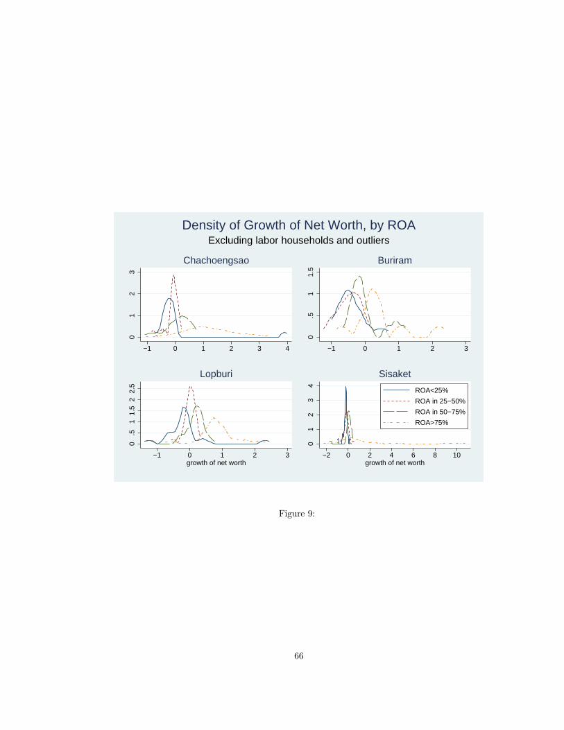
01

23

−1 0 1 2 3 4

Chachoengsao

0.5

11.

5

−1 0 1 2 3

Buriram

0.5

11.

52

2.5

−1 0 1 2 3growth of net worth

Lopburi

01

23

4

−2 0 2 4 6 8 10growth of net worth

ROA<25%

ROA in 25−50%

ROA in 50−75%

ROA>75%

Sisaket

Excluding labor households and outliersDensity of Growth of Net Worth, by ROA

Figure 9:

66

050

100

050

100

0 50 100 0 50 100

Chachoengsao Buriram

Lopburi Sisaket

95% CI Fitted values 45 degree line

Ran

k of

mea

n(R

OA

) se

cond

hal

f

Rank of mean(ROA) first half

Graphs by changwat

excluding labor householdsPersistence of ROA

Figure 10:

67

7000

0090

0000

Phy

sica

l Ass

ets

0 12 24 36 48 60 72 84month

Chachoengsao

4000

0080

0000

Phy

sica

l Ass

ets

0 12 24 36 48 60 72 84month

Buriram

7000

0010

0000

0P

hysi

cal A

sset

s

0 12 24 36 48 60 72 84month

Lopburi

1600

0022

0000

Phy

sica

l Ass

ets

0 12 24 36 48 60 72 84month

Sisaket

High ROA group, different scaleMean Value of Physical Assets

Figure 11:

68

5200

000

6200

000

Phy

sica

l Ass

ets

0 12 24 36 48 60 72 84month

Chachoengsao

6500

0080

0000

Phy

sica

l Ass

ets

0 12 24 36 48 60 72 84month

Buriram

2200

000

2600

000

Phy

sica

l Ass

ets

0 12 24 36 48 60 72 84month

Lopburi

6400

0072

0000

Phy

sica

l Ass

ets

0 12 24 36 48 60 72 84month

Sisaket

Middle ROA group, different scaleMean Value of Physical Assets

Figure 12:

69

5000

0020

0000

0F

inan

cial

Ass

ets

0 12 24 36 48 60 72 84month

Chachoengsao

1500

0030

0000

Fin

anci

al A

sset

s

0 12 24 36 48 60 72 84month

Buriram

2000

0010

0000

0F

inan

cial

Ass

ets

0 12 24 36 48 60 72 84month

Lopburi

8000

013

0000

Fin

anci

al A

sset

s

0 12 24 36 48 60 72 84month

Sisaket

Middle ROA group, different scaleMean Value of financial Assets

Figure 13:

70

02

46

8

10 12 14 16 18 20log(K)

MPKInterest rate

Marginal product of capital versus interest rate

Figure 14:

71

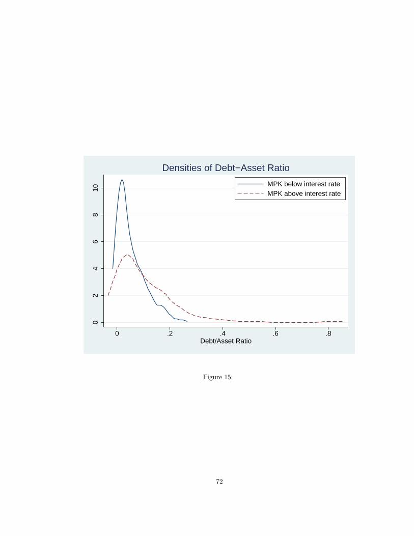
02

46

810

0 .2 .4 .6 .8Debt/Asset Ratio

MPK below interest rateMPK above interest rate

Densities of Debt−Asset Ratio

Figure 15:

72

100

200

300

400

500

Milk

per

cow

(ki

logr

ams

per

mon

th)

0 12 24 36 48 60 72 84month

−20

000

020

000

4000

0

0 12 24 36 48 60 72 84month

Net Income

Consumption

Savings

5010

015

020

0W

ealth

(*1

0,00

0)

0 12 24 36 48 60 72 84month

Case Study Household

Figure 16:

73