Embed Size (px)
Citation preview

Weakly Coupled Stochastic Decision SystemsKamesh MunagalaDuke University
(joint work with Sudiptio Guha, UPenn and Peng Shi, Duke)
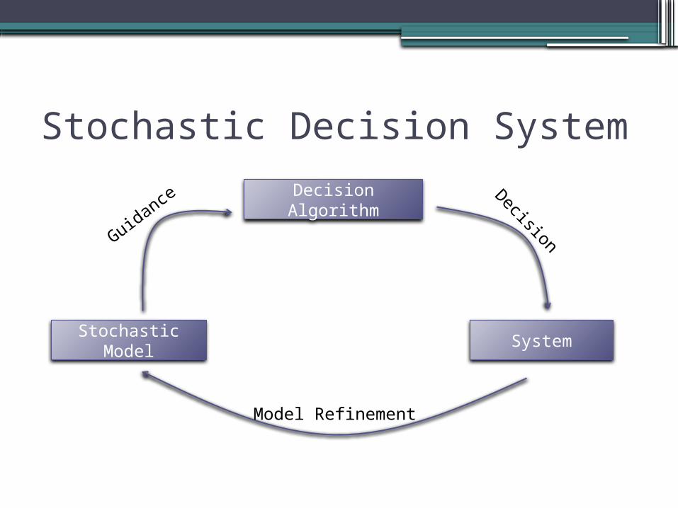
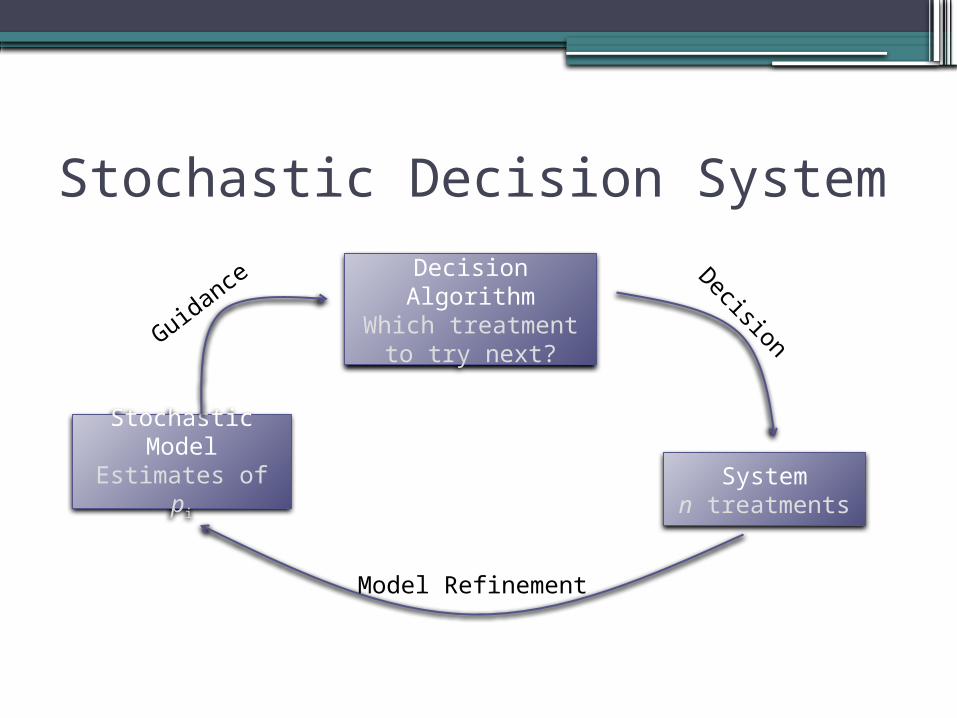
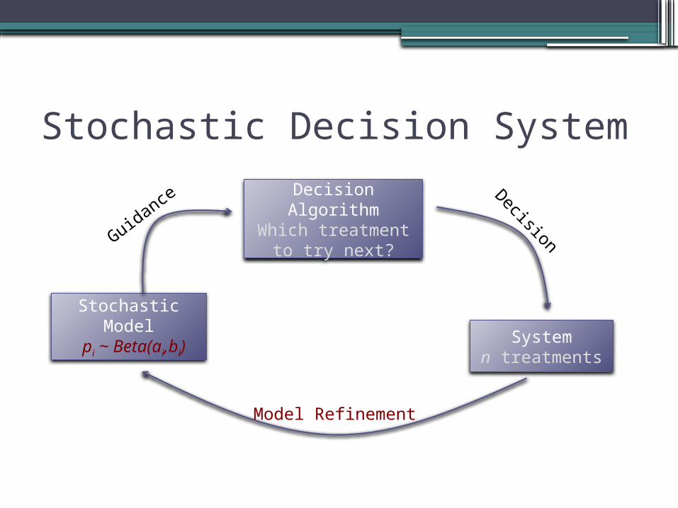
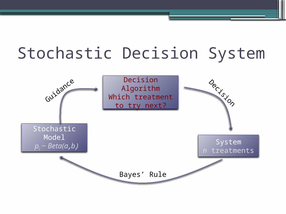
Stochastic Decision System
Decision Algorithm
Stochastic Model
System
Decision
Model Refinement
Guidan
ce
Example 1: Multi-armed Bandits
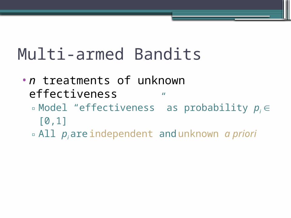
Multi-armed Bandits
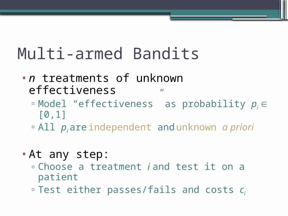
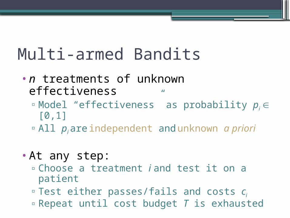
•n treatments of unknown effectiveness▫Model “effectiveness” as probability pi [0,1]
▫All pi are independent and unknown a priori
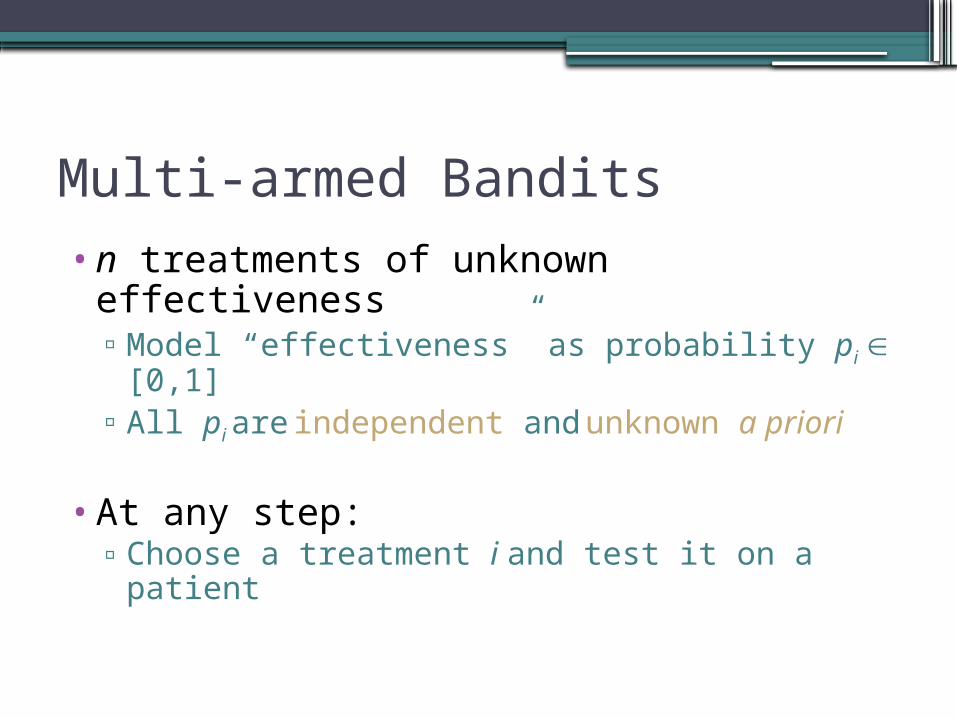
Multi-armed Bandits•n treatments of unknown effectiveness
▫Model “effectiveness” as probability pi [0,1] ▫All pi are independent and unknown a priori
•At any step:▫Choose a treatment i and test it on a patient
Multi-armed Bandits•n treatments of unknown effectiveness
▫Model “effectiveness” as probability pi [0,1] ▫All pi are independent and unknown a priori
•At any step:▫Choose a treatment i and test it on a patient▫Test either passes/fails and costs ci

Multi-armed Bandits•n treatments of unknown effectiveness
▫Model “effectiveness” as probability pi [0,1] ▫All pi are independent and unknown a priori
•At any step:▫Choose a treatment i and test it on a patient▫Test either passes/fails and costs ci
▫Repeat until cost budget T is exhausted
Multi-armed Bandits•n treatments of unknown effectiveness
▫Model “effectiveness” as probability pi [0,1] ▫All pi are independent and unknown a priori
•At any step:▫Choose a treatment i and test it on a patient▫Test either passes/fails and costs ci
▫Repeat until cost budget T is exhausted
•Choose best treatment/treatments for marketing
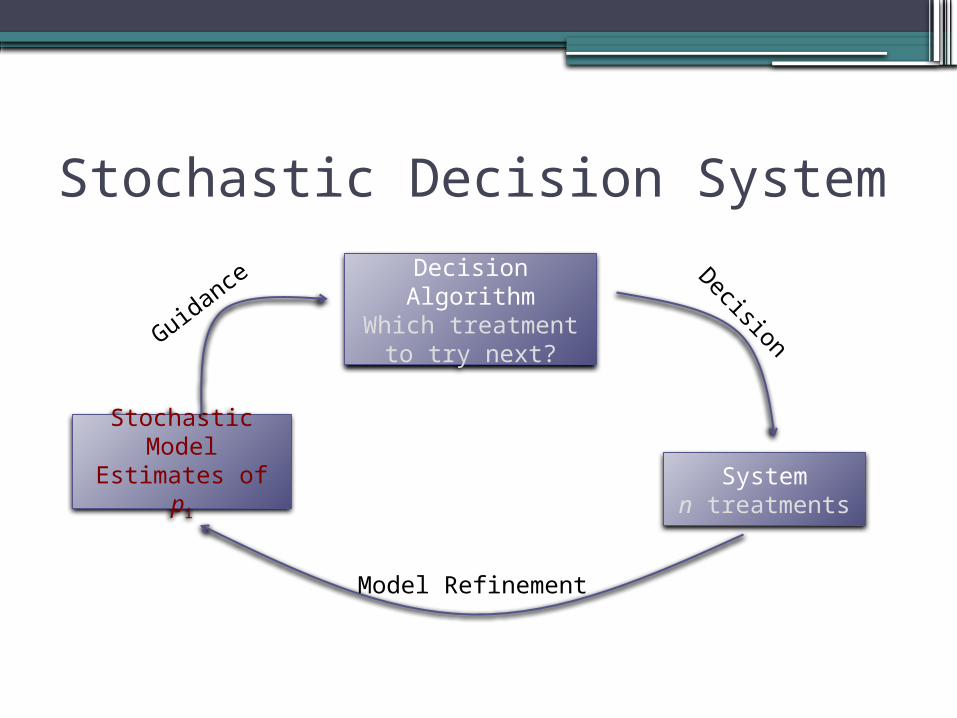
Stochastic Decision System
Decision Algorithm
Which treatment to try next?
Stochastic Model
Estimates of piSystem
n treatments
Decision
Model Refinement
Guidan
ce
Stochastic Decision System
Decision Algorithm
Which treatment to try next?
Stochastic Model
Estimates of piSystem
n treatments
Decision
Model Refinement
Guidan
ce
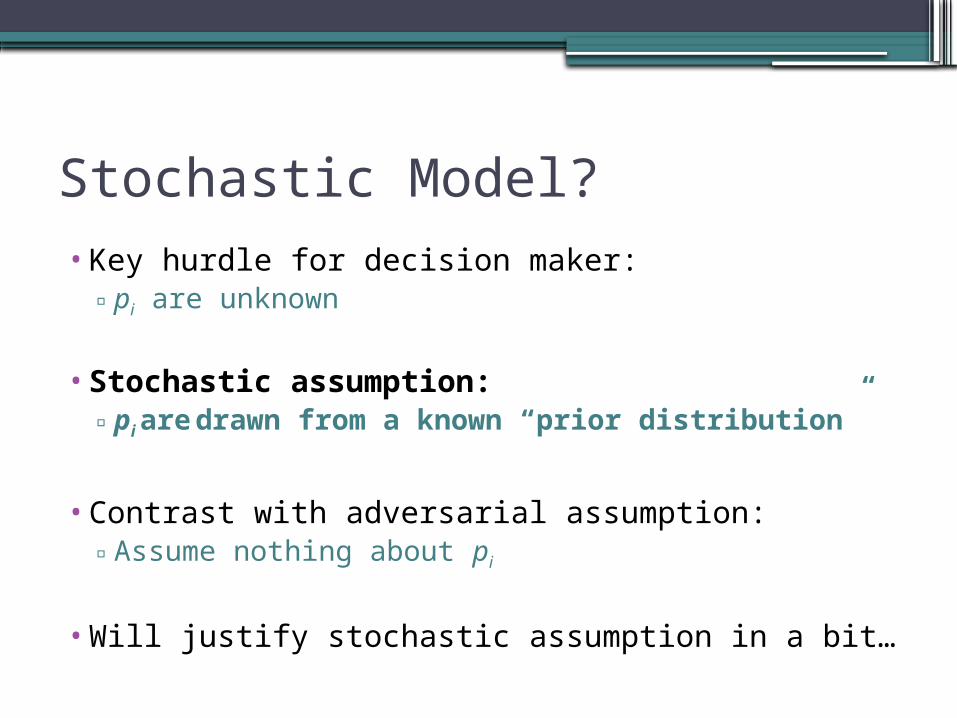
Stochastic Model?• Key hurdle for decision maker:
▫ pi are unknown
• Stochastic assumption: ▫ pi are drawn from a known “prior distribution”
• Contrast with adversarial assumption:▫Assume nothing about pi
• Will justify stochastic assumption in a bit…
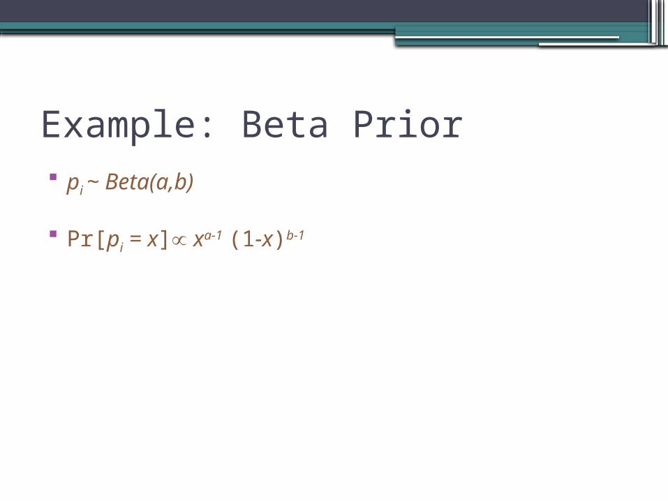
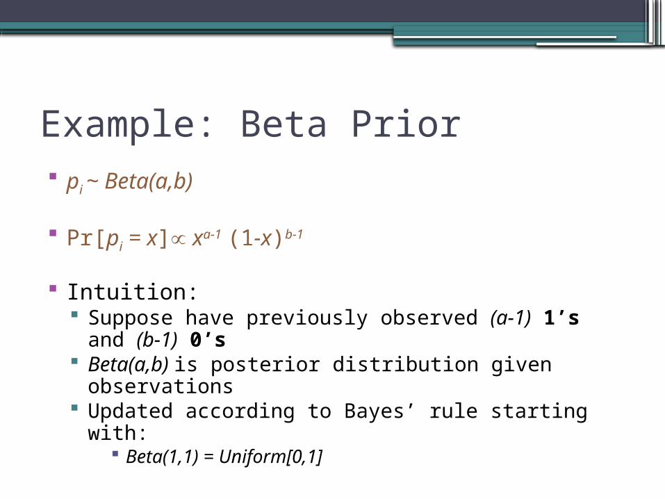
Example: Beta Prior pi ~ Beta(a,b)
Pr[pi = x] xa-1 (1-x)b-1
Example: Beta Prior pi ~ Beta(a,b)
Pr[pi = x] xa-1 (1-x)b-1
Intuition: Suppose have previously observed (a-1) 1’s and (b-1)
0’s Beta(a,b) is posterior distribution given observations Updated according to Bayes’ rule starting with:
Beta(1,1) = Uniform[0,1]
Expected Reward = E[pi] = a/(a+b)
Stochastic Decision System
Decision Algorithm
Which treatment to try next?
Stochastic Model
pi ~ Beta(ai,bi)System
n treatments
Decision
Model Refinement
Guidan
ce
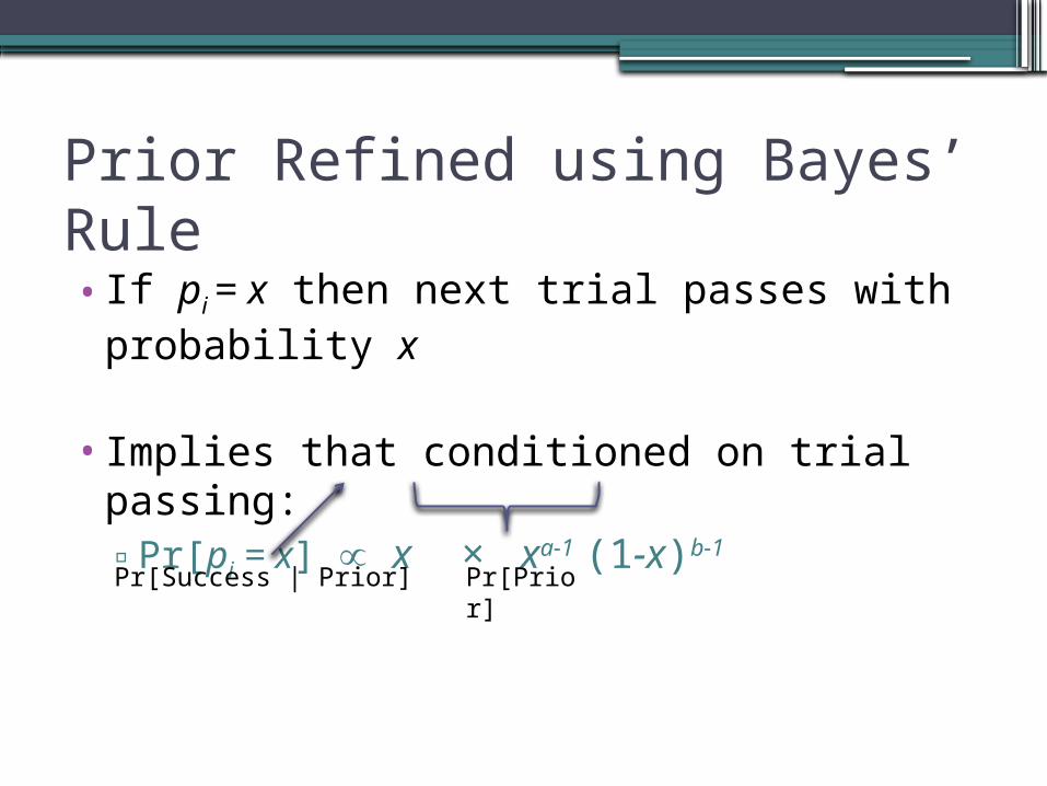
Prior Refined using Bayes’ Rule
•If pi = x then next trial passes with probability x
•Implies that conditioned on trial passing:▫Pr[pi = x] x × xa-1 (1-x)b-1
Pr[Success | Prior] Pr[Prior]
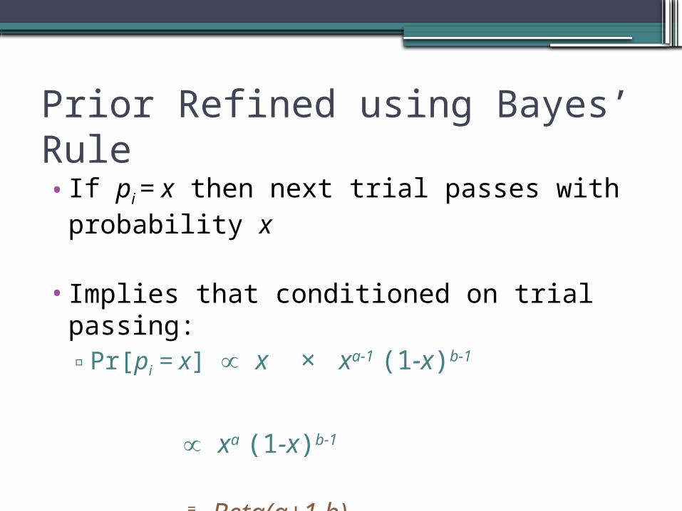
Prior Refined using Bayes’ Rule
•If pi = x then next trial passes with probability x
•Implies that conditioned on trial passing:▫Pr[pi = x] x × xa-1 (1-x)b-1
xa (1-x)b-1
= Beta(a+1,b)
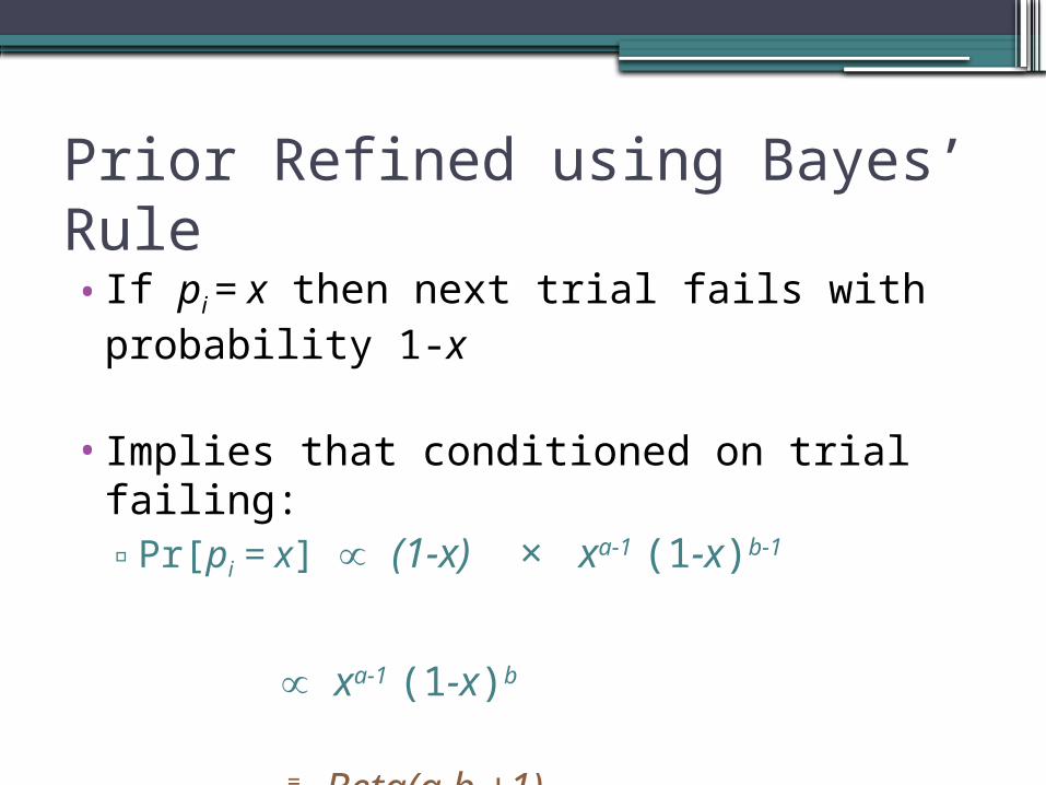
Prior Refined using Bayes’ Rule
•If pi = x then next trial fails with probability 1-x
•Implies that conditioned on trial failing:▫Pr[pi = x] (1-x) × xa-1 (1-x)b-1
xa-1 (1-x)b
= Beta(a,b +1)
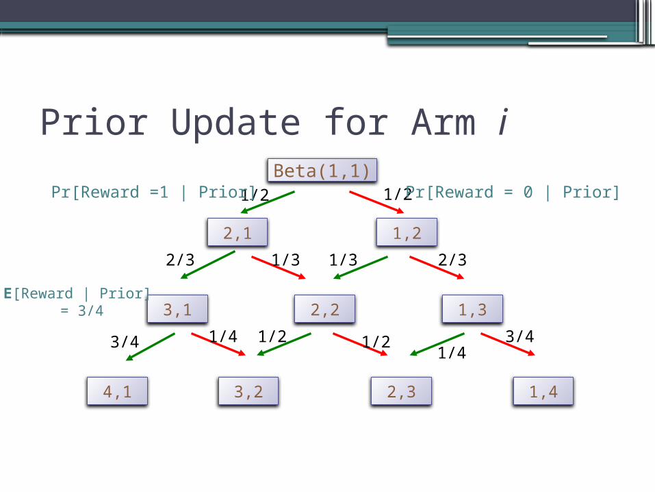
Prior Update for Arm iBeta(1,1)
2,1 1,2
2,23,1 1,3
3,2 2,3 1,44,1
1/2 1/2
2/3 1/3 1/3 2/3
3/4 1/4
1/21/21/43/4
Pr[Reward = 0 | Prior]Pr[Reward =1 | Prior]
E[Reward | Prior] = 3/4
Multi-armed Bandit Lingo
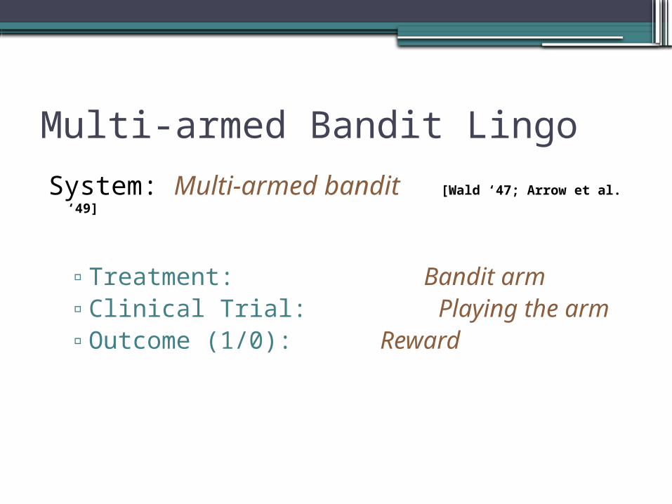
System: Multi-armed bandit [Wald ‘47; Arrow et al. ‘49]
▫Treatment: Bandit arm▫Clinical Trial: Playing the arm▫Outcome (1/0): Reward
Convenient Abstraction
•Posterior density of arm captured by:▫Observed rewards from arm so far▫Called the “state” of the arm
Convenient Abstraction
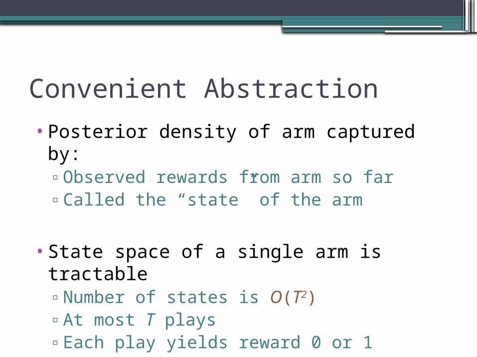
•Posterior density of arm captured by:▫Observed rewards from arm so far▫Called the “state” of the arm
•State space of a single arm is tractable▫Number of states is O(T2)▫At most T plays▫Each play yields reward 0 or 1
Stochastic Decision System
Decision Algorithm
Which treatment to try next?
Stochastic Model
pi ~ Beta(ai,bi)System
n treatments
Decision
Bayes’ Rule
Guidan
ce
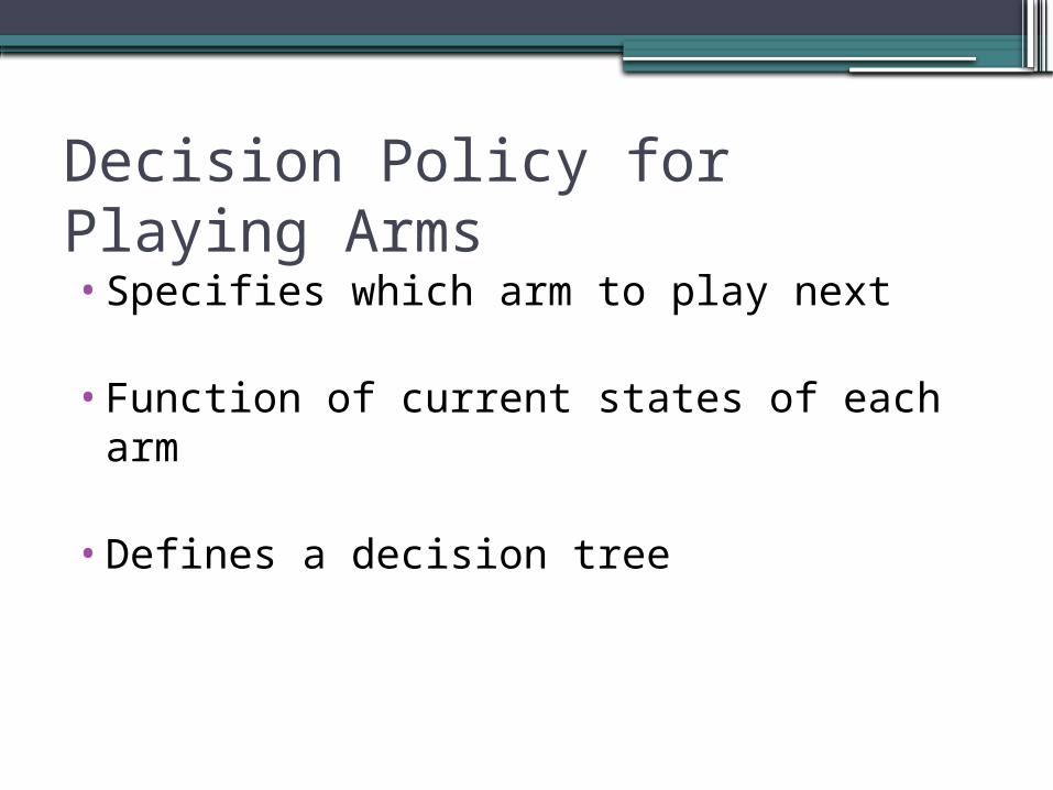
Decision Policy for Playing Arms•Specifies which arm to play next
•Function of current states of each arm
•Defines a decision tree
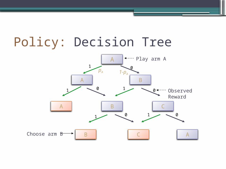
Policy: Decision TreeA
A B
BA C
B C A
Play arm A1
1 1
11
0
0
00
0 Observed Reward
Choose arm B
pA 1-pA
Goal
•Find decision policy with maximum value:
▫Value = E [ Reward of chosen arm ]
▫What is expectation over?
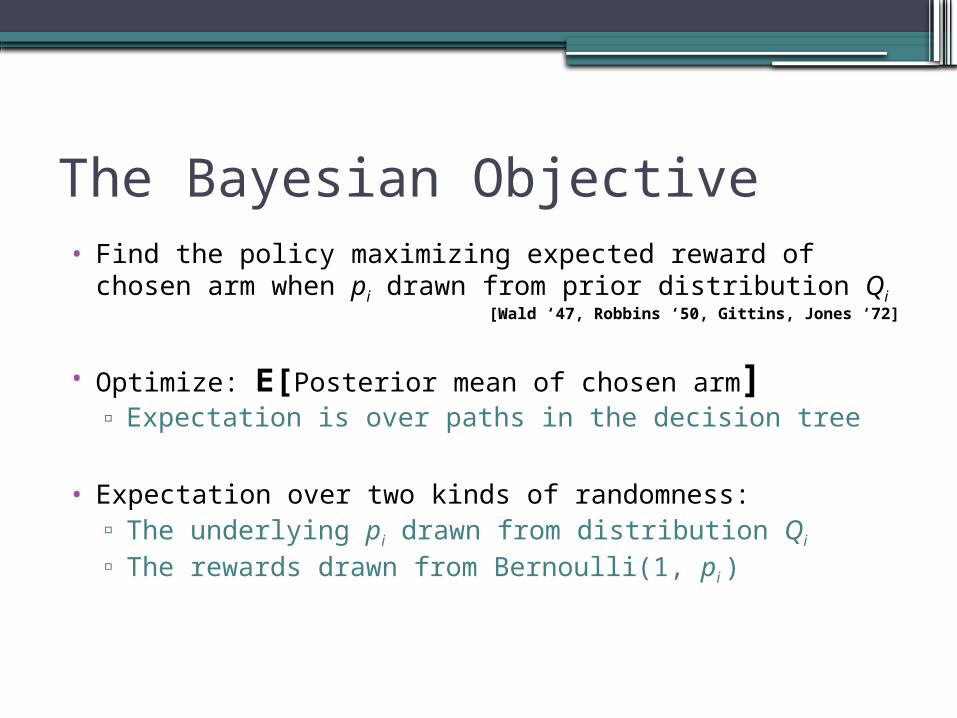
The Bayesian Objective• Find the policy maximizing expected reward of chosen arm
when pi drawn from prior distribution Qi[Wald ‘47, Robbins ‘50, Gittins, Jones ‘72]
• Optimize: E[Posterior mean of chosen arm]▫ Expectation is over paths in the decision tree
The Bayesian Objective• Find the policy maximizing expected reward of chosen arm
when pi drawn from prior distribution Qi[Wald ‘47, Robbins ‘50, Gittins, Jones ‘72]
• Optimize: E[Posterior mean of chosen arm]▫ Expectation is over paths in the decision tree
• Expectation over two kinds of randomness:▫ The underlying pi drawn from distribution Qi
▫ The rewards drawn from Bernoulli(1, pi )
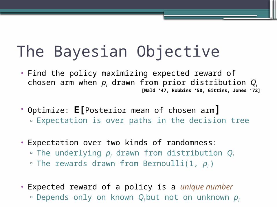
• Expected reward of a policy is a unique number▫ Depends only on known Qi but not on unknown pi
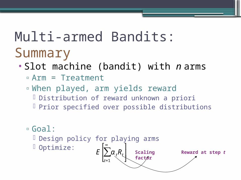
Multi-armed Bandits: Summary
•Slot machine (bandit) with n arms ▫Arm = Treatment▫When played, arm yields reward
Distribution of reward unknown a priori Prior specified over possible distributions
▫Goal: Design policy for playing arms Optimize:
€
E α tRt
t=1
∞
∑ ⎡
⎣ ⎢
⎤
⎦ ⎥ Reward at step tScaling
factor
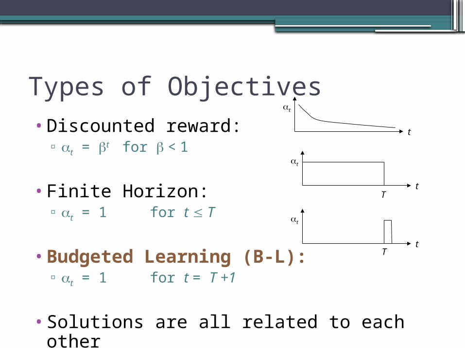
Types of Objectives•Discounted reward:
▫ t = t for < 1
•Finite Horizon:▫ t = 1 for t T
•Budgeted Learning (B-L):▫ t = 1 for t = T +1
•Solutions are all related to each other
t
t
t
t
t
t
T
T
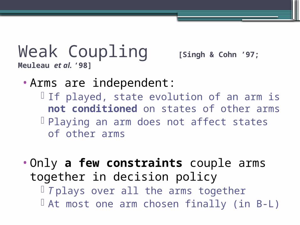
Weak Coupling [Singh & Cohn ’97; Meuleau et al. ‘98]
•Arms are independent: If played, state evolution of an arm is not
conditioned on states of other arms Playing an arm does not affect states of other
arms
•Only a few constraints couple arms together in decision policy
T plays over all the arms together At most one arm chosen finally (in B-L)
Space of Decision Policies
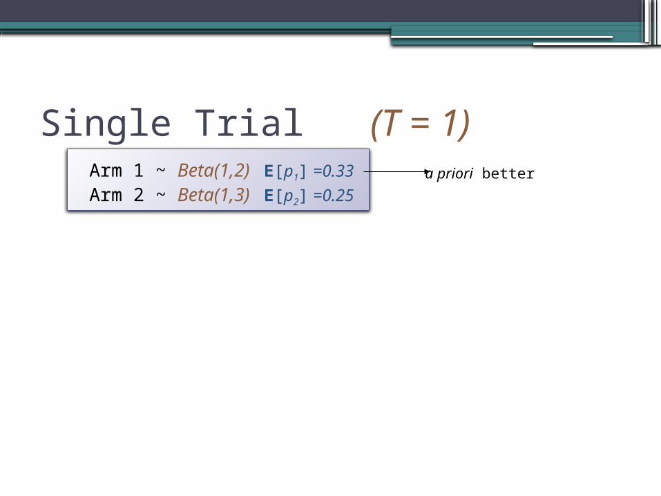
Single Trial (T = 1) Arm 1 ~ Beta(1,2) E[p1] =0.33
Arm 2 ~ Beta(1,3) E[p2] =0.25a priori better
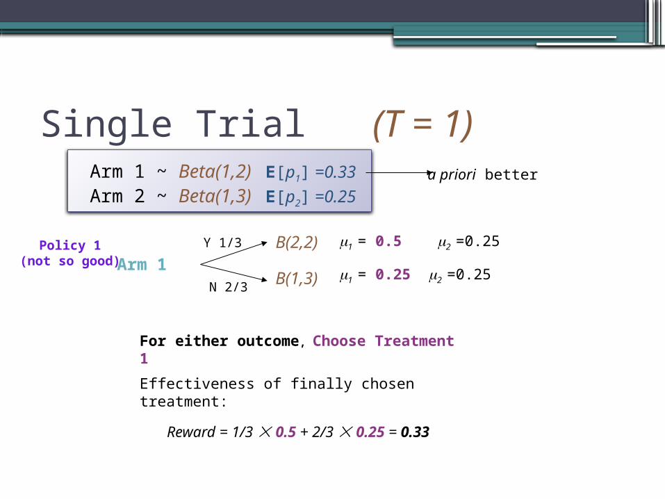
Single Trial (T = 1)
Arm 1 Y 1/3
N 2/3
B(2,2)
B(1,3)
For either outcome, Choose Treatment 1
Effectiveness of finally chosen treatment:
Reward = 1/3 0.5 + 2/3 0.25 = 0.33
Policy 1(not so good)
Arm 1 ~ Beta(1,2) E[p1] =0.33
Arm 2 ~ Beta(1,3) E[p2] =0.25a priori better
1 = 0.5 2 =0.25
1 = 0.25 2 =0.25
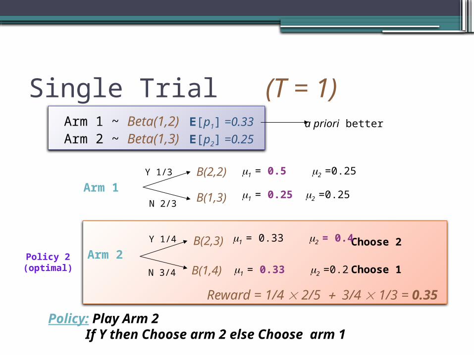
Single Trial (T = 1)
Arm 2 Y 1/4
N 3/4
B(2,3)
B(1,4)
Policy: Play Arm 2 If Y then Choose arm 2 else Choose arm 1
Reward = 1/4 2/5 3/4 1/3 = 0.35
Policy 2(optimal)
Choose 2
Choose 1
Arm 1 Y 1/3
N 2/3
B(2,2)
B(1,3)
Arm 1 ~ Beta(1,2) E[p1] =0.33
Arm 2 ~ Beta(1,3) E[p2] =0.25a priori better
1 = 0.5 2 =0.25
1 = 0.25 2 =0.25
1 = 0.33 2 = 0.4
1 = 0.33 2 =0.2

T = 2: Adaptive Solution
Play Arm 1
Y 1/2
p1 ~ B(1,1) p2 ~ B(5,2) p3 ~ B(21,11)
N 1/2
p1 ~ B(2,1) Play Arm 1
p1 ~ B(1,2) Play Arm 2
Y 2/3
N 1/3
p1 ~ B(3,1) Choose 1
p1 ~ B(2,2) Choose 2
Y 5/7
N 2/7
p2 ~ B(6,2) Choose 2
p2 ~ B(5,3) Choose 3
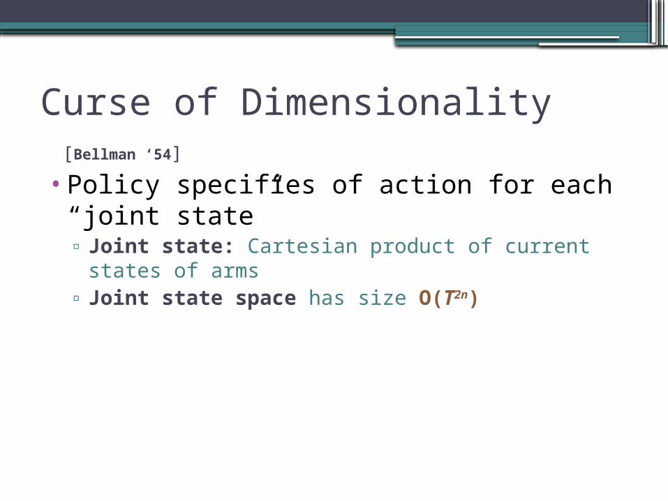
Curse of Dimensionality [Bellman
‘54]
•Policy specifies of action for each “joint state”▫ Joint state: Cartesian product of current states of
arms▫ Joint state space has size O(T2n)
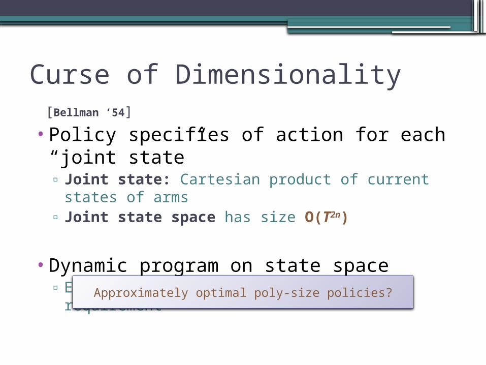
Curse of Dimensionality [Bellman
‘54]
•Policy specifies of action for each “joint state”▫ Joint state: Cartesian product of current states of
arms▫ Joint state space has size O(T2n)
•Dynamic program on state space▫ Exponential running time and space requirement
Approximately optimal poly-size policies?
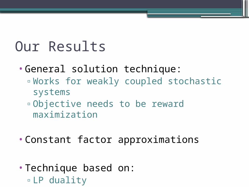
Our Results
•General solution technique:▫Works for weakly coupled stochastic
systems▫Objective needs to be reward maximization
•Constant factor approximations
•Technique based on:▫LP duality▫Markov’s inequality
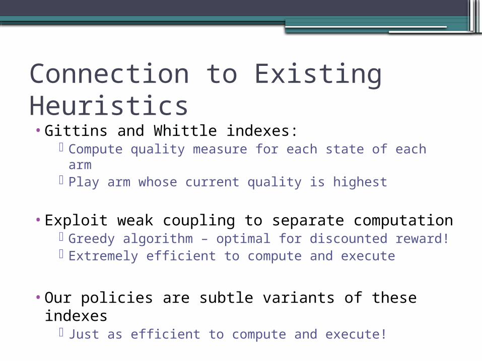
Connection to Existing Heuristics•Gittins and Whittle indexes:
Compute quality measure for each state of each arm Play arm whose current quality is highest
•Exploit weak coupling to separate computation Greedy algorithm – optimal for discounted reward! Extremely efficient to compute and execute
•Our policies are subtle variants of these indexes Just as efficient to compute and execute!

Solution Overview (STOC ‘07)
Solution Idea
•Consider any decision policy P
•Consider its behavior restricted to arm i
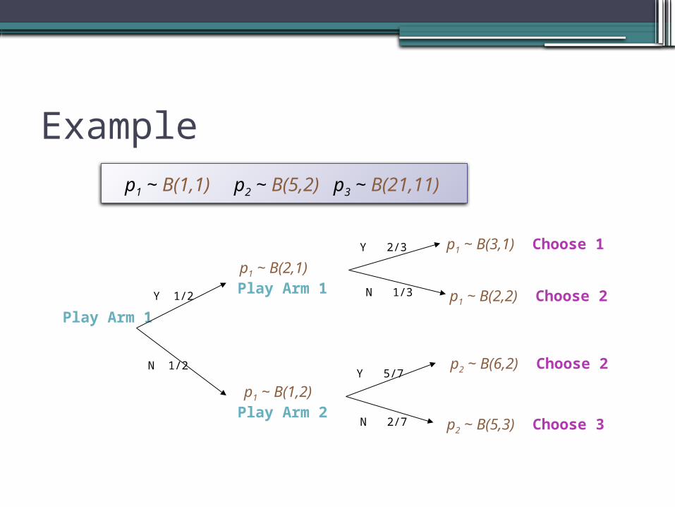
Example
Play Arm 1
Y 1/2
p1 ~ B(1,1) p2 ~ B(5,2) p3 ~ B(21,11)
N 1/2
p1 ~ B(2,1) Play Arm 1
p1 ~ B(1,2) Play Arm 2
Y 2/3
N 1/3
p1 ~ B(3,1) Choose 1
p1 ~ B(2,2) Choose 2
Y 5/7
N 2/7
p2 ~ B(6,2) Choose 2
p2 ~ B(5,3) Choose 3
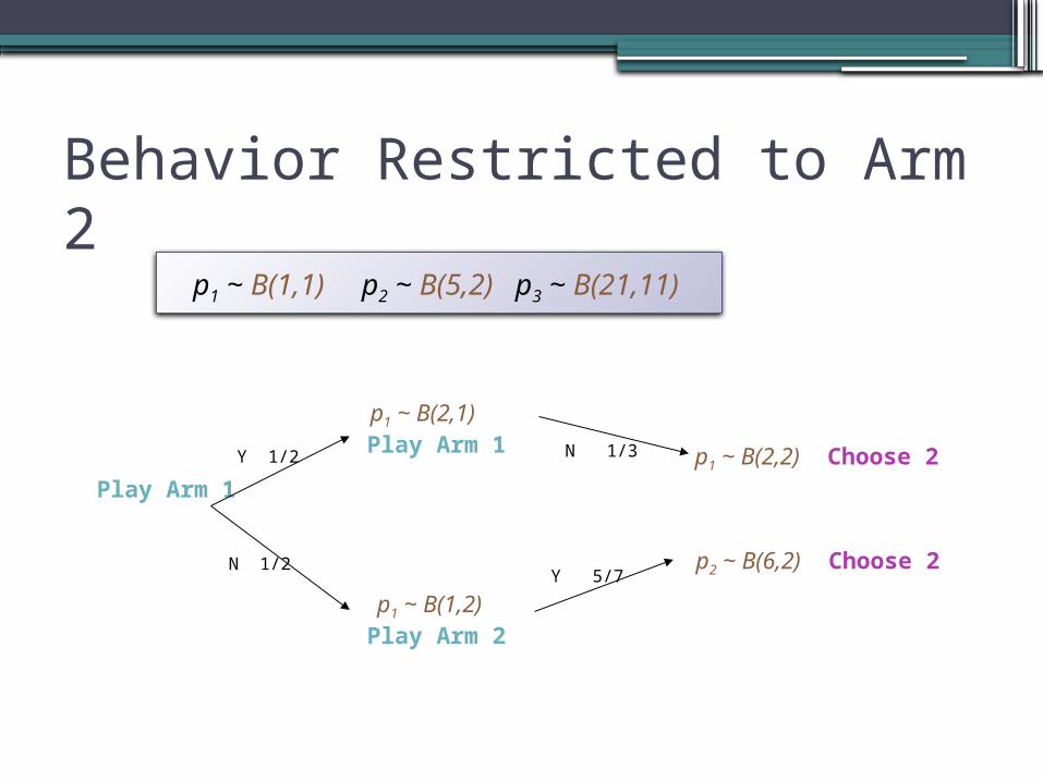
Behavior Restricted to Arm 2
Play Arm 1
Y 1/2
p1 ~ B(1,1) p2 ~ B(5,2) p3 ~ B(21,11)
N 1/2
p1 ~ B(2,1) Play Arm 1
p1 ~ B(1,2) Play Arm 2
N 1/3 p1 ~ B(2,2) Choose 2
Y 5/7p2 ~ B(6,2) Choose 2
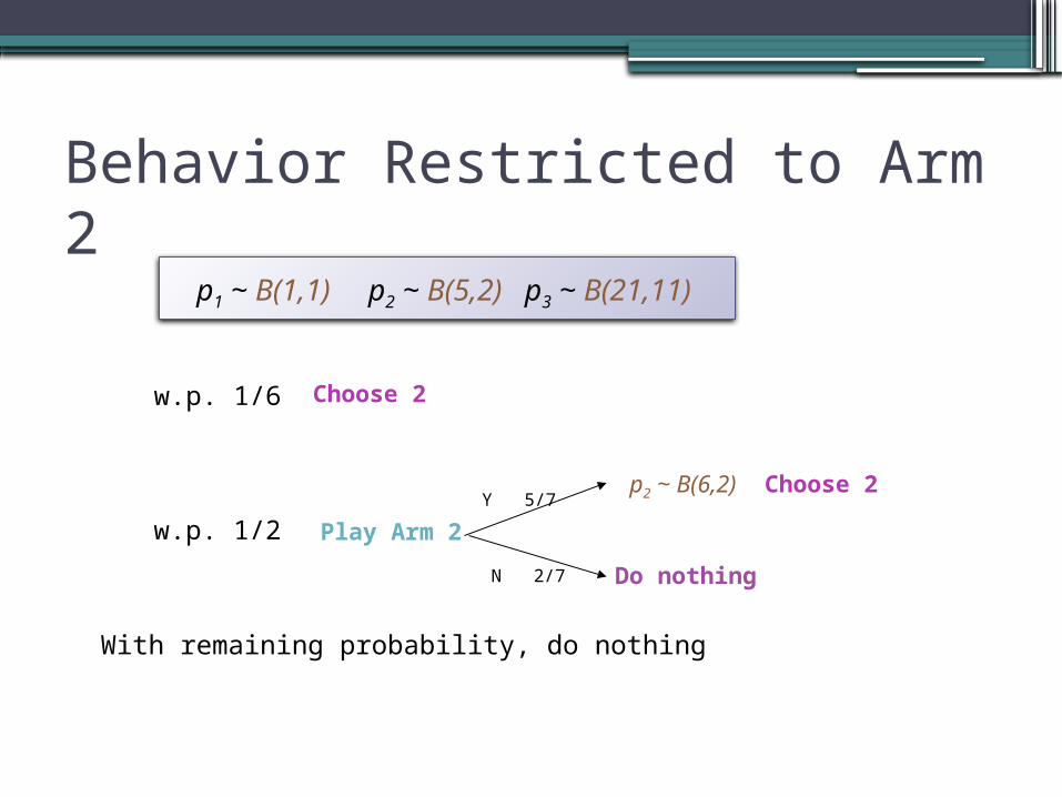
Behavior Restricted to Arm 2p1 ~ B(1,1) p2 ~ B(5,2) p3 ~ B(21,11)
Play Arm 2
Choose 2
Y 5/7p2 ~ B(6,2) Choose 2
w.p. 1/2
w.p. 1/6
With remaining probability, do nothing
N 2/7 Do nothing
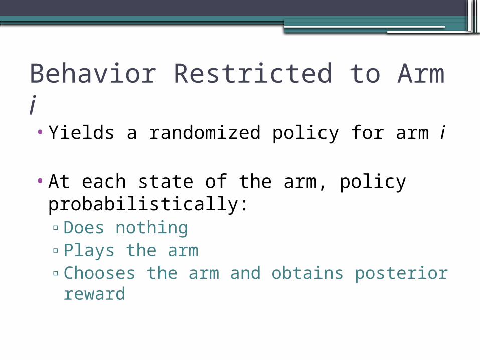
Behavior Restricted to Arm i
•Yields a randomized policy for arm i
•At each state of the arm, policy probabilistically:▫Does nothing▫Plays the arm▫Chooses the arm and obtains posterior
reward
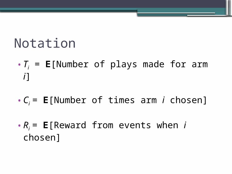
Notation
•Ti = E[Number of plays made for arm i]
•Ci = E[Number of times arm i chosen]
•Ri = E[Reward from events when i chosen]
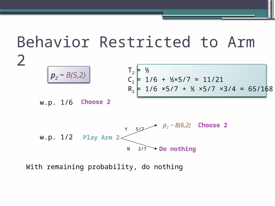
Behavior Restricted to Arm 2
Play Arm 2
Choose 2
Y 5/7p2 ~ B(6,2) Choose 2
w.p. 1/2
w.p. 1/6
With remaining probability, do nothing
N 2/7 Do nothing
T2 = ½C2 = 1/6 + ½×5/7 = 11/21R2 = 1/6 ×5/7 + ½ ×5/7 ×3/4 = 65/168
p2 ~ B(5,2)
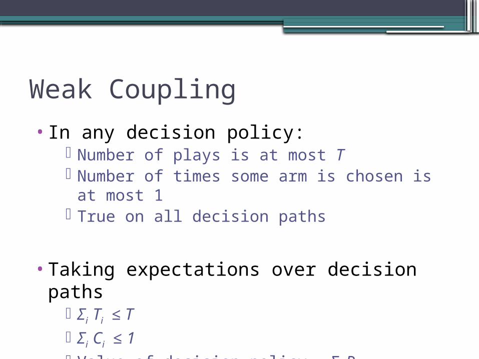
Weak Coupling
•In any decision policy: Number of plays is at most T Number of times some arm is chosen is at
most 1 True on all decision paths
•Taking expectations over decision paths Σi Ti ≤ T Σi Ci ≤ 1 Value of decision policy = Σi Ri
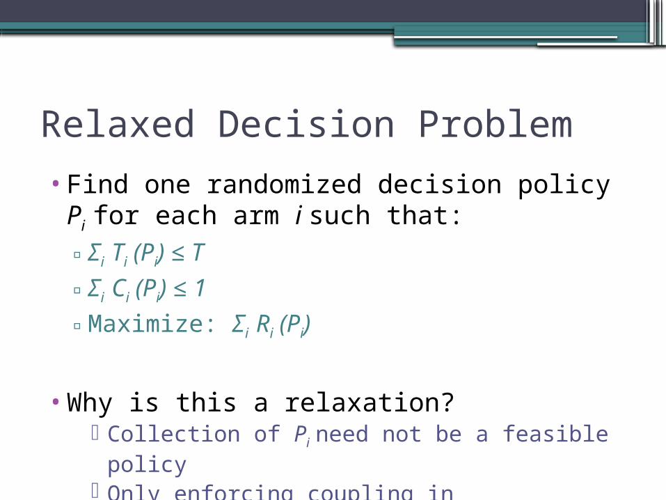
Relaxed Decision Problem
•Find one randomized decision policy Pi for each arm i such that:▫Σi Ti (Pi) ≤ T
▫Σi Ci (Pi) ≤ 1
▫Maximize: Σi Ri (Pi)
•Why is this a relaxation? Collection of Pi need not be a feasible policy Only enforcing coupling in expectation!
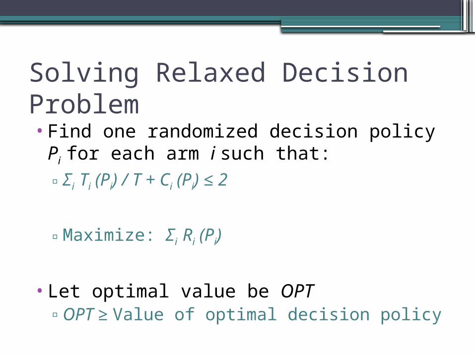
Solving Relaxed Decision Problem•Find one randomized decision policy Pi for
each arm i such that:▫Σi Ti (Pi) / T + Ci (Pi) ≤ 2
▫Maximize: Σi Ri (Pi)
•Let optimal value be OPT▫OPT ≥ Value of optimal decision policy
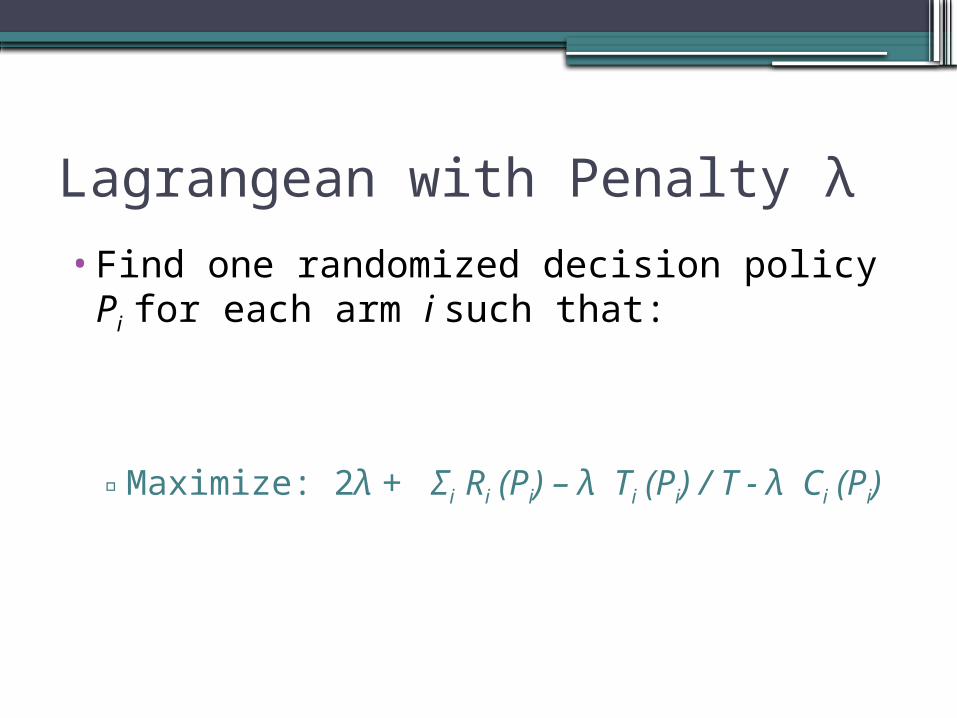
Lagrangean with Penalty λ
•Find one randomized decision policy Pi for each arm i such that:
▫Maximize: 2λ + Σi Ri (Pi) – λ Ti (Pi) / T - λ Ci (Pi)
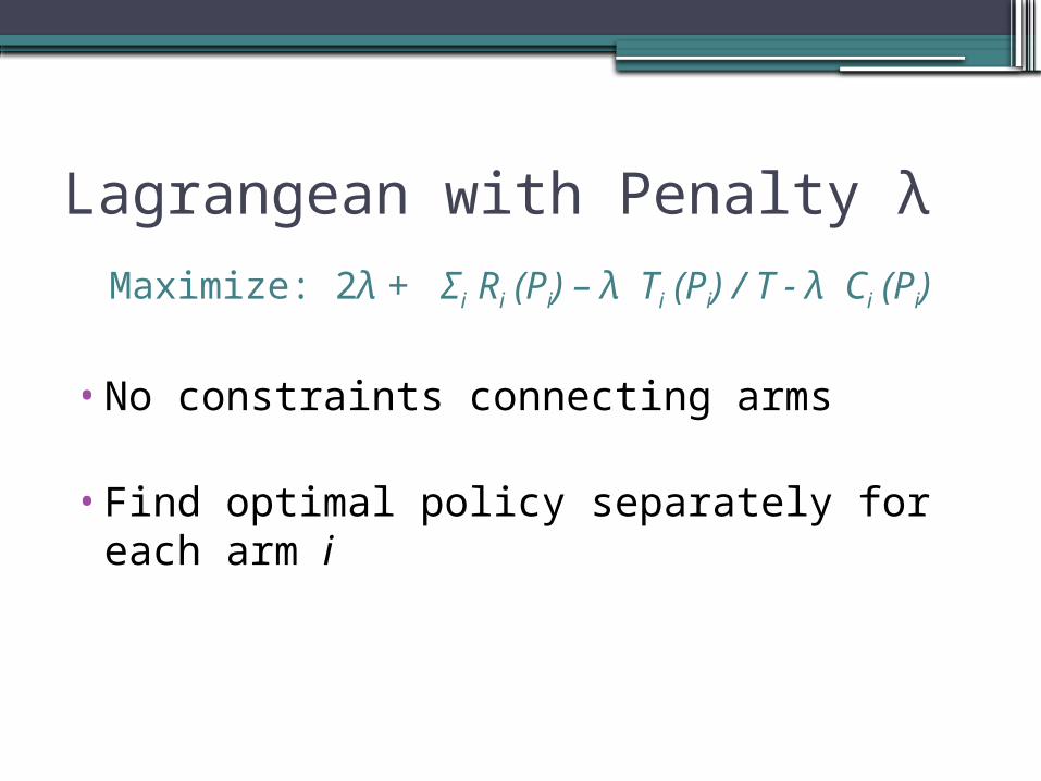
Lagrangean with Penalty λ
Maximize: 2λ + Σi Ri (Pi) – λ Ti (Pi) / T - λ Ci (Pi)
•No constraints connecting arms
•Find optimal policy separately for each arm i
Lagrangean with Penalty λ
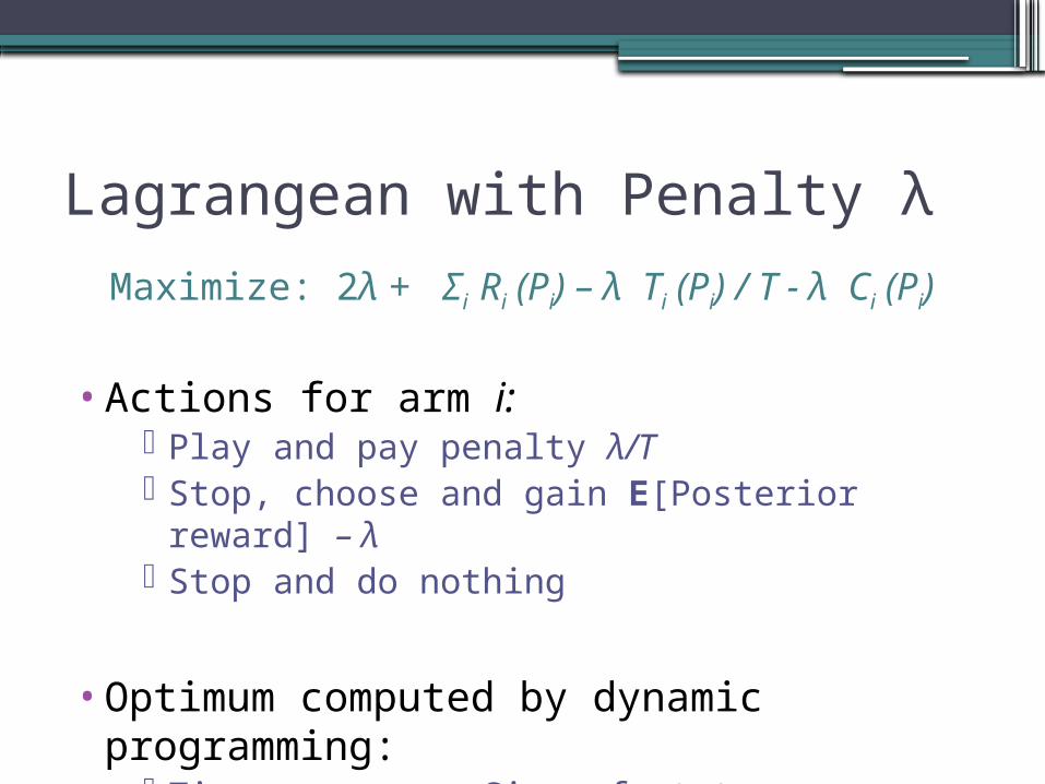
Maximize: 2λ + Σi Ri (Pi) – λ Ti (Pi) / T - λ Ci (Pi)
•Actions for arm i: Play and pay penalty λ/T Stop, choose and gain E[Posterior reward] –
λ Stop and do nothing
•Optimum computed by dynamic programming:
Time per arm = Size of state space = O(T2)
Weak Duality
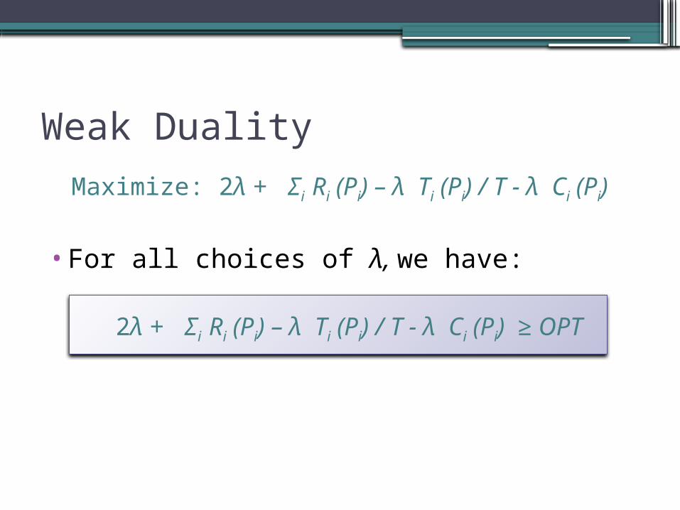
Maximize: 2λ + Σi Ri (Pi) – λ Ti (Pi) / T - λ Ci (Pi)
•For all choices of λ, we have:
2λ + Σi Ri (Pi) – λ Ti (Pi) / T - λ Ci (Pi) ≥ OPT
Choice of λ
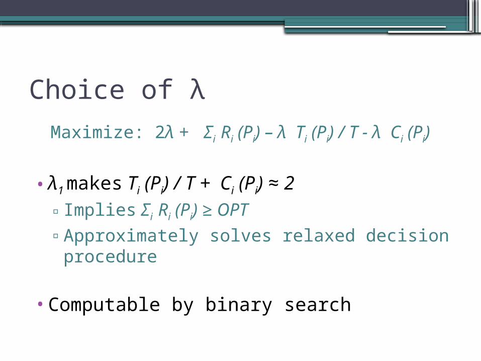
Maximize: 2λ + Σi Ri (Pi) – λ Ti (Pi) / T - λ Ci (Pi)
•λ1 makes Ti (Pi) / T + Ci (Pi) ≈ 2▫Implies Σi Ri (Pi) ≥ OPT▫Approximately solves relaxed decision
procedure
•Computable by binary search
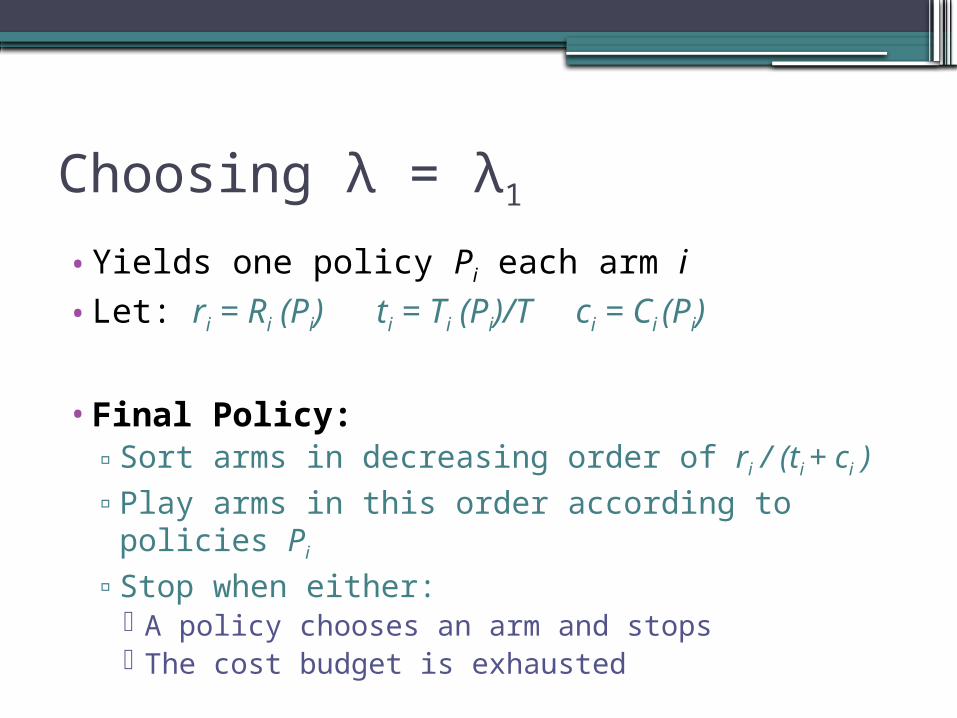
Choosing λ = λ1
•Yields one policy Pi each arm i
•Let: ri = Ri (Pi) ti = Ti (Pi)/T ci = Ci (Pi)
•Final Policy:▫Sort arms in decreasing order of ri / (ti + ci )▫Play arms in this order according to policies
Pi
▫Stop when either: A policy chooses an arm and stops The cost budget is exhausted
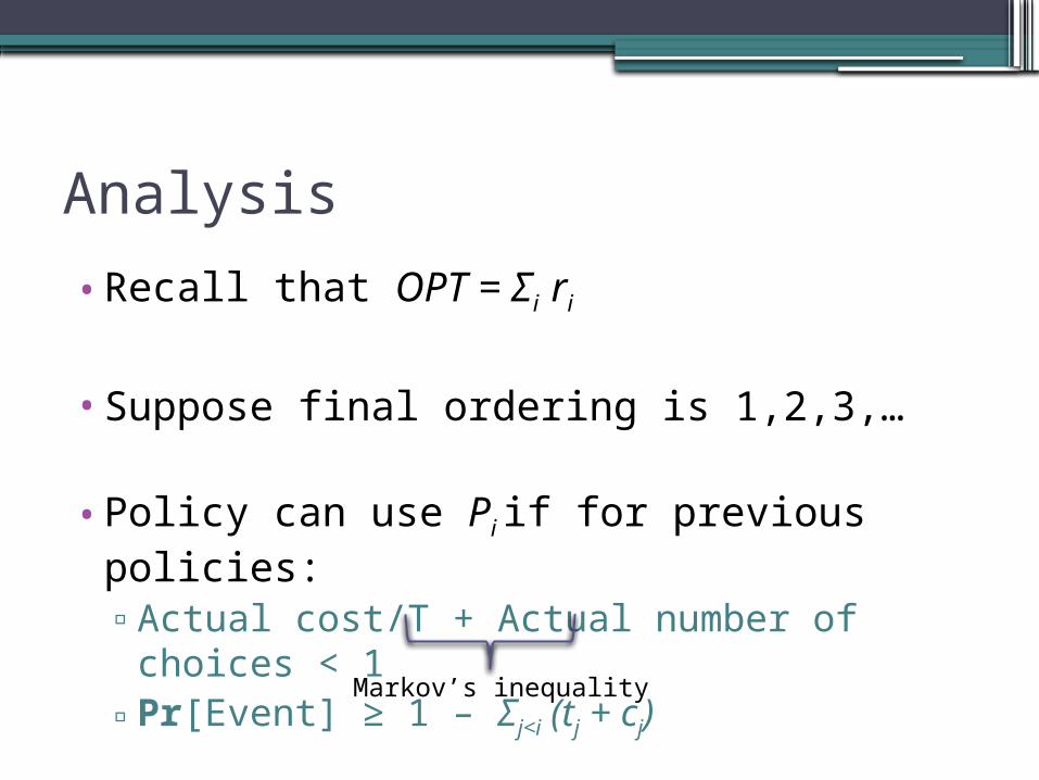
Analysis
•Recall that OPT = Σi ri
•Suppose final ordering is 1,2,3,…
•Policy can use Pi if for previous policies:▫Actual cost/T + Actual number of choices <
1▫Pr[Event] ≥ 1 – Σj<i (tj + cj) Markov’s inequality
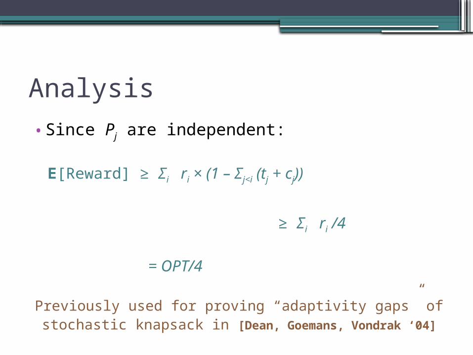
Analysis
•Since Pj are independent:
E[Reward] ≥ Σi ri × (1 – Σj<i (tj + cj))
≥ Σi ri /4
= OPT/4
Previously used for proving “adaptivity gaps” of stochastic knapsack in [Dean, Goemans, Vondrak ‘04]
More Examples: MAB Problems
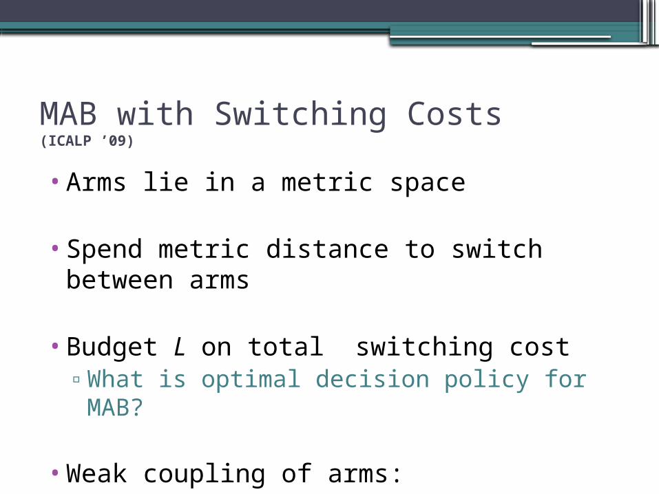
MAB with Switching Costs (ICALP ’09)
•Arms lie in a metric space
•Spend metric distance to switch between arms
•Budget L on total switching cost▫What is optimal decision policy for MAB?
•Weak coupling of arms:▫Three coupling constraints instead of 2
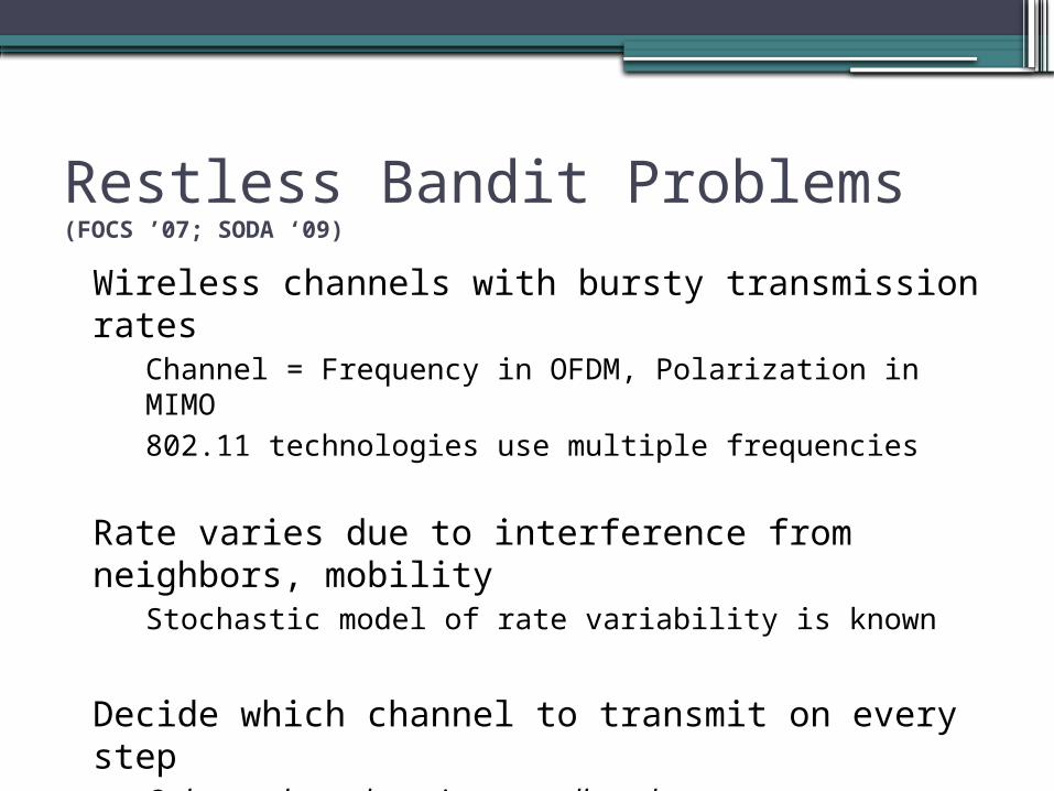
Restless Bandit Problems (FOCS ’07;
SODA ‘09)
Wireless channels with bursty transmission ratesChannel = Frequency in OFDM, Polarization in MIMO802.11 technologies use multiple frequencies
Rate varies due to interference from neighbors, mobility
Stochastic model of rate variability is known
Decide which channel to transmit on every stepOnly one channel per time step allowedMaximize throughput = Time-average transmission rate
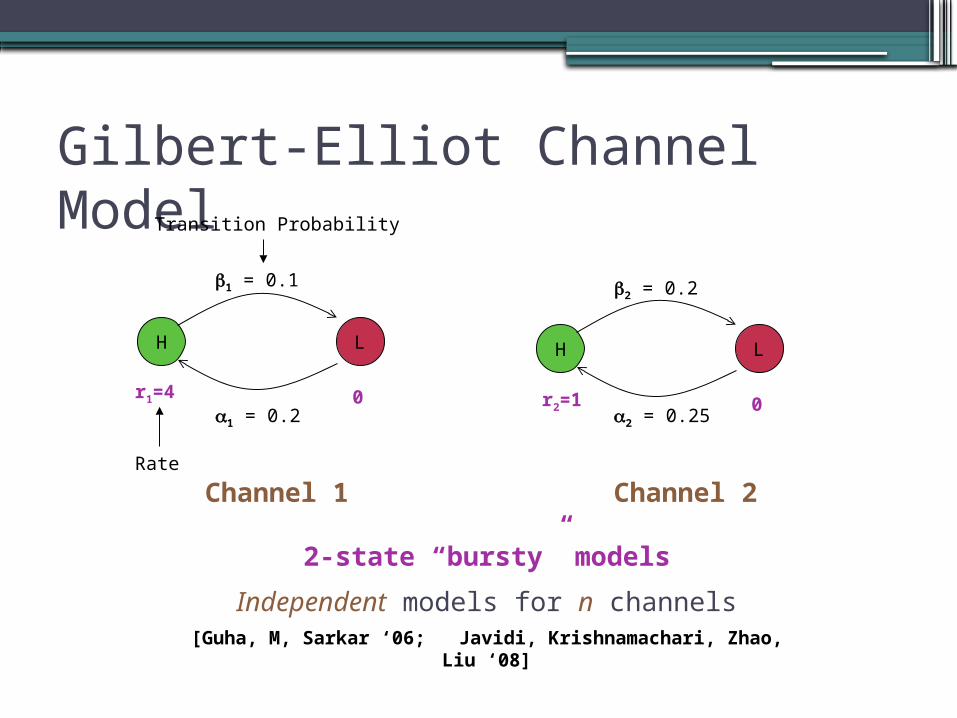
Gilbert-Elliot Channel Model
H L
1 = 0.1
1 = 0.2
2-state “bursty” models
Independent models for n channels[Guha, M, Sarkar ‘06; Javidi, Krishnamachari, Zhao, Liu ‘08]
r1=4 0
Transition Probability
Rate
H L
2 = 0.2
2 = 0.25r2=1 0
Channel 1 Channel 2
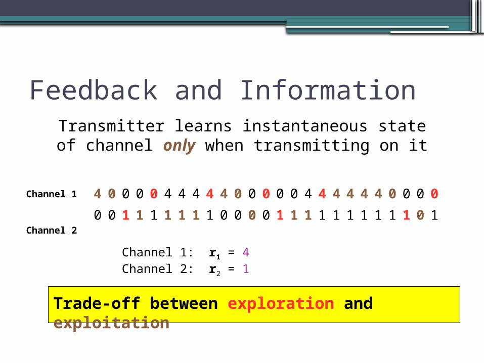
Feedback and InformationTransmitter learns instantaneous state of
channel only when transmitting on it
4 0 0 0 0 4 4 4 4 4 0 0 0 0 0 4 4 4 4 4 4 0 0 0 0
0 0 1 1 1 1 1 1 1 0 0 0 0 1 1 1 1 1 1 1 1 1 1 0 1
Channel 1
Channel 2
Channel 1: r1 = 4 Channel 2: r2 = 1
Trade-off between exploration and exploitation
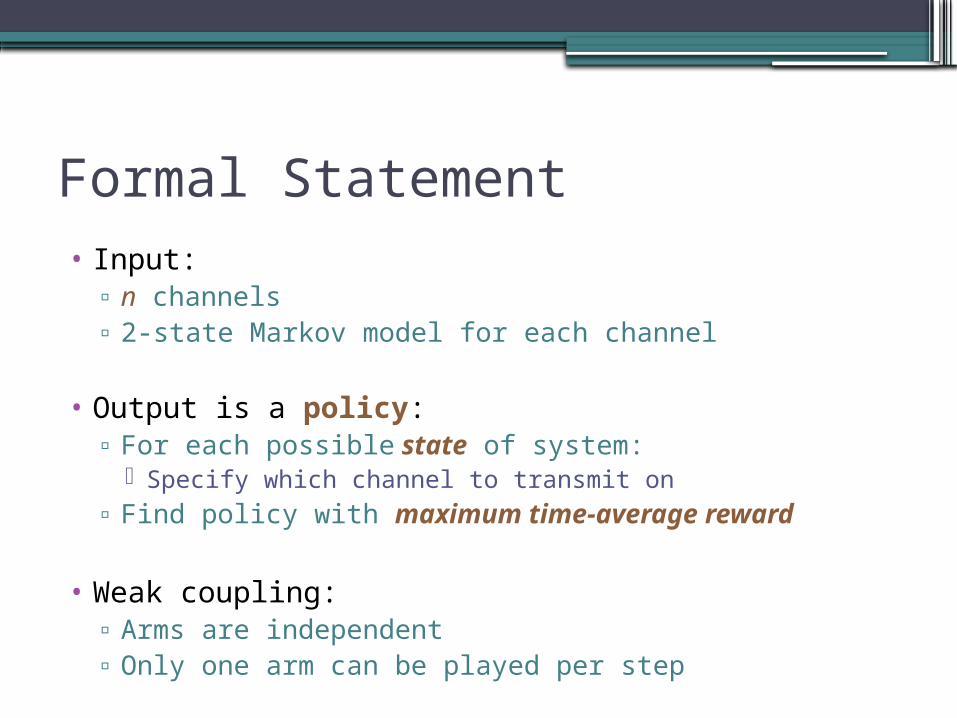
Formal Statement• Input:
▫ n channels▫ 2-state Markov model for each channel
• Output is a policy:▫ For each possible state of system:
Specify which channel to transmit on▫ Find policy with maximum time-average reward
• Weak coupling:▫ Arms are independent▫ Only one arm can be played per step
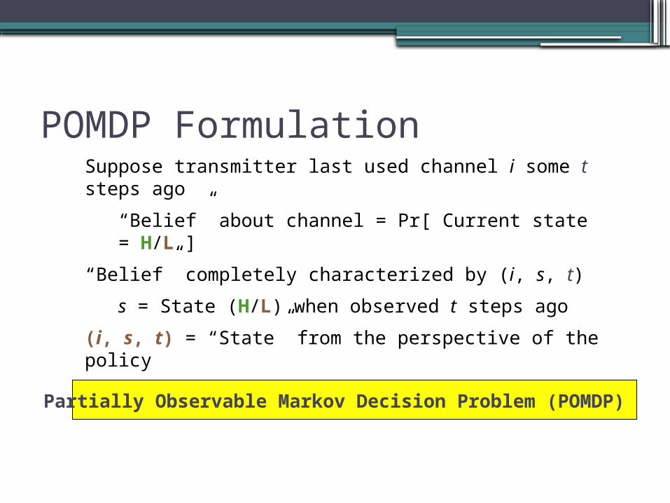
POMDP FormulationSuppose transmitter last used channel i some t steps ago
“Belief” about channel = Pr[ Current state = H/L ]
“Belief” completely characterized by (i, s, t)
s = State (H/L) when observed t steps ago
(i, s, t) = “State” from the perspective of the policy
Partially Observable Markov Decision Problem (POMDP)
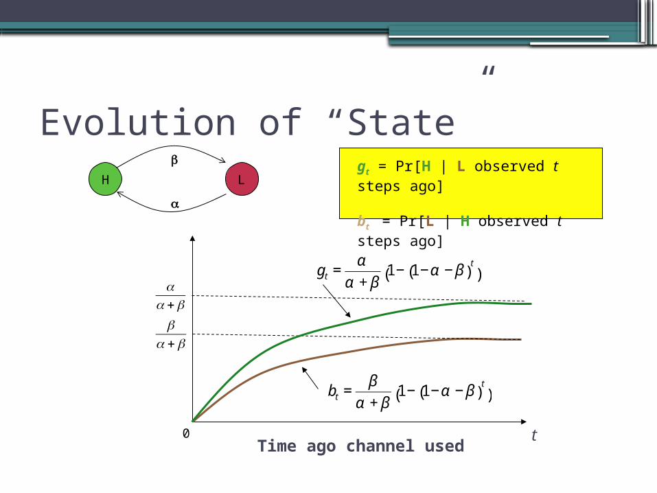
Evolution of “State”
t0
€
βα +β
€
bt =β
α + β1− 1−α − β( )
t
( )
Time ago channel used
gt = Pr[H | L observed t steps ago]
bt = Pr[L | H observed t steps ago]
H L
€
αα +β
€
gt =α
α + β1− 1−α − β( )
t
( )
Matching Problems
Stochastic Matching (Chen et al. ’09)
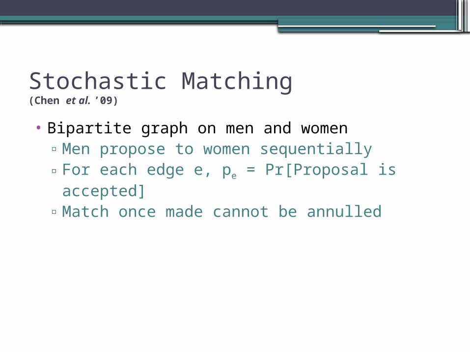
• Bipartite graph on men and women▫Men propose to women sequentially▫For each edge e, pe = Pr[Proposal is accepted]▫Match once made cannot be annulled
Stochastic Matching• Bipartite graph on men and women
▫Men propose to women sequentially▫For each edge e, pe = Pr[Proposal is accepted]▫Match once made cannot be annulled
• Decision policy:▫Optimal order in which men make proposals▫Maximize E[# successful matches]
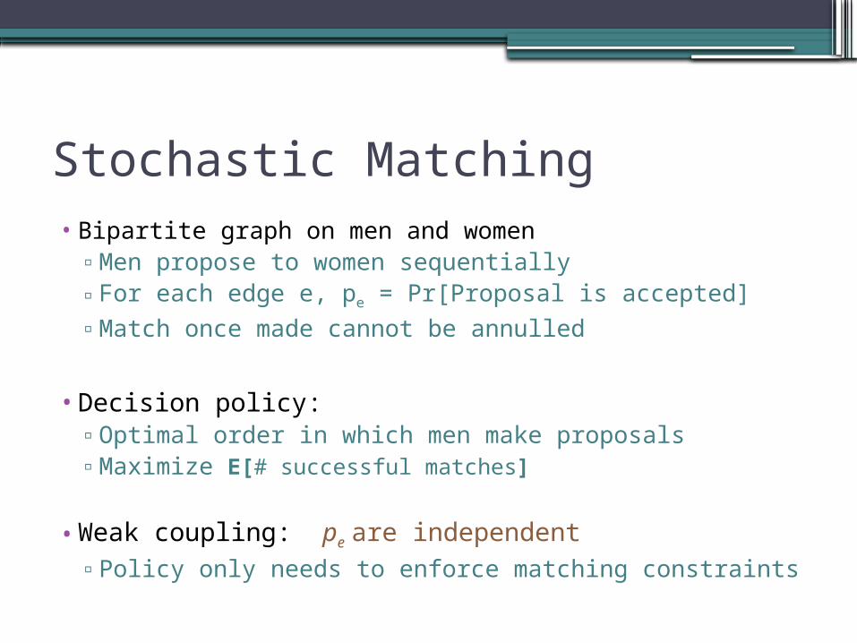
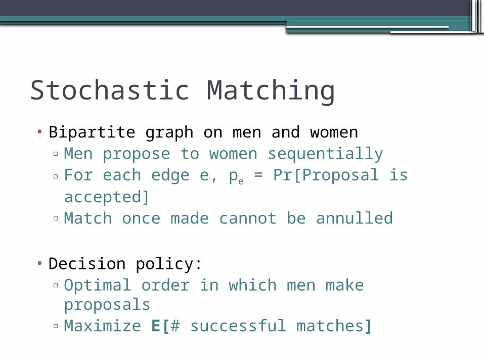
Stochastic Matching• Bipartite graph on men and women
▫Men propose to women sequentially▫For each edge e, pe = Pr[Proposal is accepted]▫Match once made cannot be annulled
• Decision policy:▫Optimal order in which men make proposals▫Maximize E[# successful matches]
• Weak coupling: pe are independent▫Policy only needs to enforce matching constraints
Budgeted Allocation
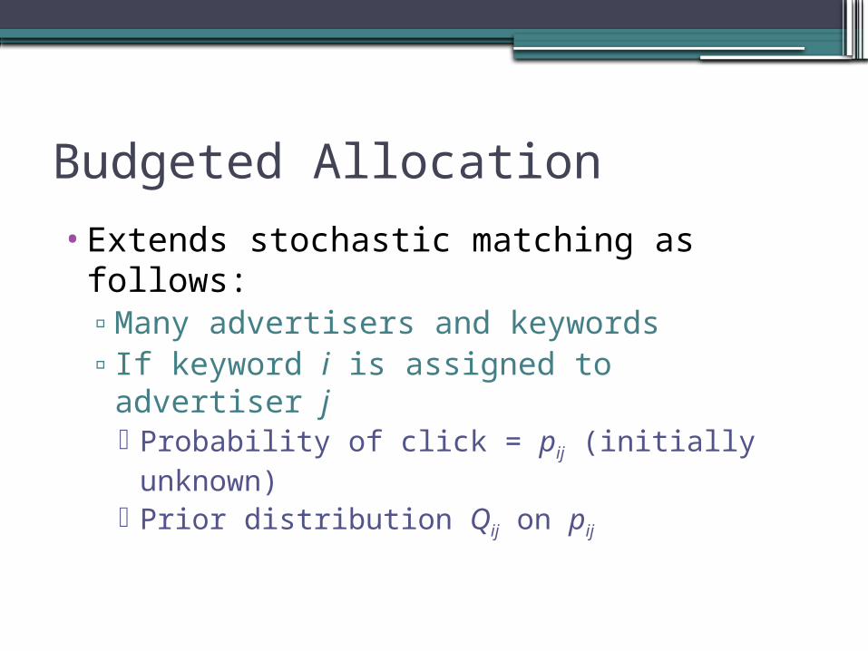
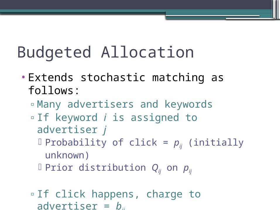
•Extends stochastic matching as follows:▫Many advertisers and keywords▫If keyword i is assigned to advertiser j Probability of click = pij (initially unknown) Prior distribution Qij on pij
Budgeted Allocation
•Extends stochastic matching as follows:▫Many advertisers and keywords▫If keyword i is assigned to advertiser j Probability of click = pij (initially unknown) Prior distribution Qij on pij
▫If click happens, charge to advertiser = bij
▫Advertiser j has budget Bj
•Keywords arrive online
Budgeted Allocation
•Decision policy:▫Decide which advertiser to allocate
keyword to▫Maximize E[Revenue of auctioneer]
Budgeted Allocation
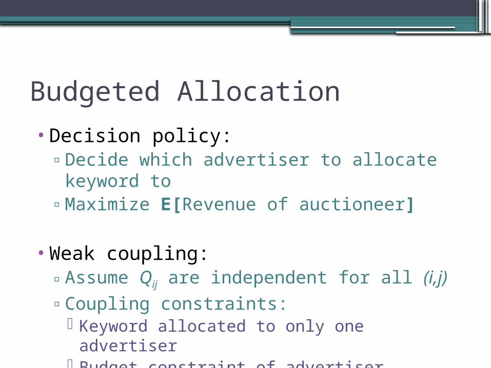
•Decision policy:▫Decide which advertiser to allocate
keyword to▫Maximize E[Revenue of auctioneer]
•Weak coupling:▫Assume Qij are independent for all (i,j)▫Coupling constraints: Keyword allocated to only one advertiser Budget constraint of advertiser
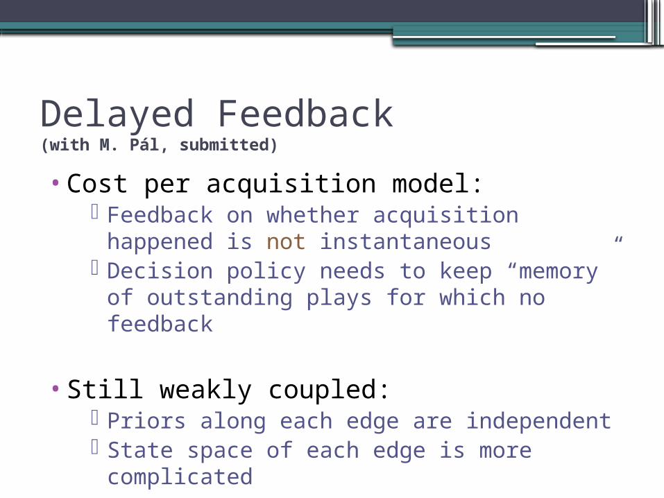
Delayed Feedback (with M. Pál, submitted)
•Cost per acquisition model: Feedback on whether acquisition happened is
not instantaneous Decision policy needs to keep “memory” of
outstanding plays for which no feedback
•Still weakly coupled: Priors along each edge are independent State space of each edge is more complicated
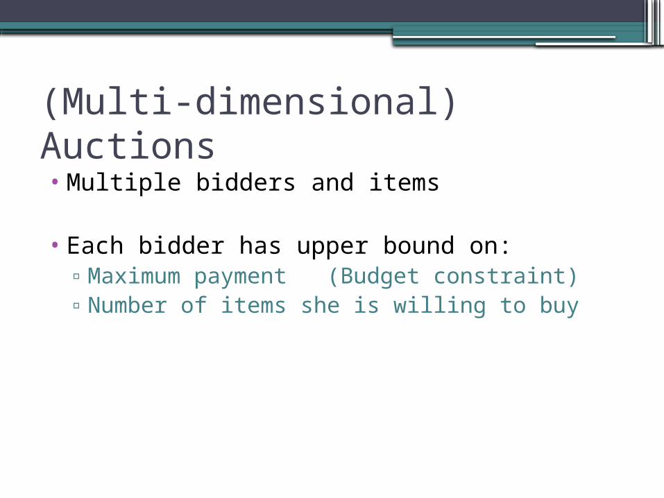
(Multi-dimensional) Auctions• Multiple bidders and items
• Each bidder has upper bound on:▫Maximum payment (Budget constraint)▫Number of items she is willing to buy
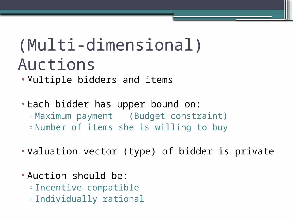
(Multi-dimensional) Auctions• Multiple bidders and items
• Each bidder has upper bound on:▫Maximum payment (Budget constraint)▫Number of items she is willing to buy
• Valuation vector (type) of bidder is private
• Auction should be:▫ Incentive compatible▫ Individually rational
Bayesian Assumption
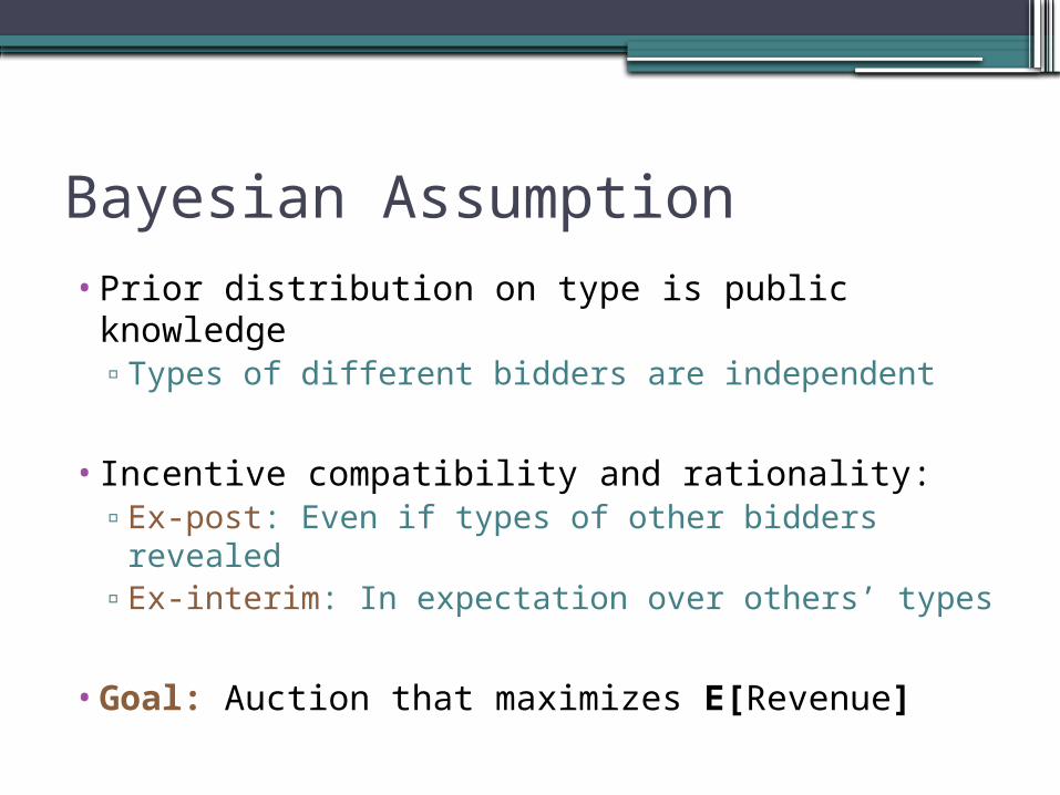
•Prior distribution on type is public knowledge▫Types of different bidders are independent
•Incentive compatibility and rationality:▫Ex-post: Even if types of other bidders
revealed▫Ex-interim: In expectation over others’ types
•Goal: Auction that maximizes E[Revenue]
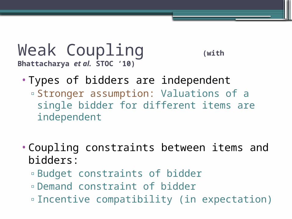
Weak Coupling (with Bhattacharya et al. STOC ‘10)
•Types of bidders are independent▫Stronger assumption: Valuations of a single
bidder for different items are independent
•Coupling constraints between items and bidders:▫Budget constraints of bidder▫Demand constraint of bidder▫Incentive compatibility (in expectation)
Contrast with Other Models
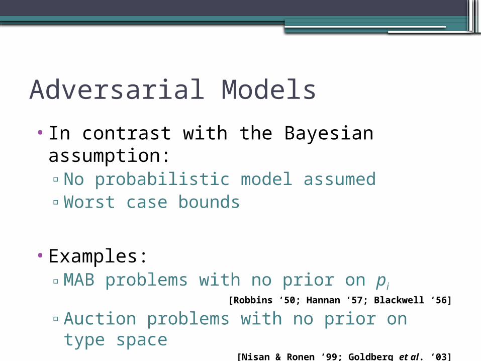
Adversarial Models
•In contrast with the Bayesian assumption:▫No probabilistic model assumed▫Worst case bounds
•Examples:▫MAB problems with no prior on pi
[Robbins ‘50; Hannan ‘57; Blackwell ‘56]
▫Auction problems with no prior on type space
[Nisan & Ronen ’99; Goldberg et al. ‘03]
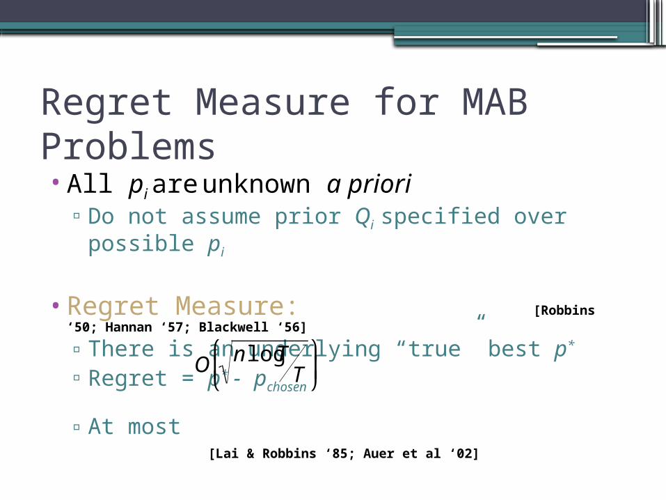
Regret Measure for MAB Problems•All pi are unknown a priori
▫Do not assume prior Qi specified over possible pi
•Regret Measure: [Robbins ‘50; Hannan ‘57; Blackwell ‘56]
▫There is an underlying “true” best p*
▫Regret = p* - pchosen
▫At most [Lai & Robbins ‘85; Auer et al ‘02]
•Meaningful when n is small and T is large▫What about small time horizons?
€
O n logTT
⎛
⎝ ⎜
⎞
⎠ ⎟
Advantages of Regret Measure•Works “as is” for a large class of problems
▫In fact, does not need weak coupling assumption▫However, does need a large time horizon
•Related to algorithms for convex optimization▫Algorithms based on “regularization”▫Well-developed theory and techniques
•Minimal assumptions on system▫Who gives us the prior?
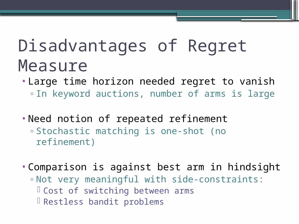
Disadvantages of Regret Measure•Large time horizon needed regret to vanish
▫In keyword auctions, number of arms is large
•Need notion of repeated refinement▫Stochastic matching is one-shot (no refinement)
•Comparison is against best arm in hindsight▫Not very meaningful with side-constraints: Cost of switching between arms Restless bandit problems
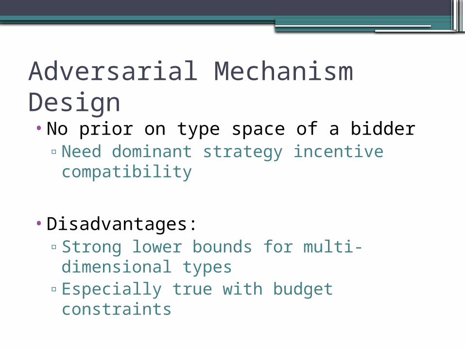
Adversarial Mechanism Design
•No prior on type space of a bidder▫Need dominant strategy incentive
compatibility
•Disadvantages:▫Strong lower bounds for multi-dimensional
types▫Especially true with budget constraints
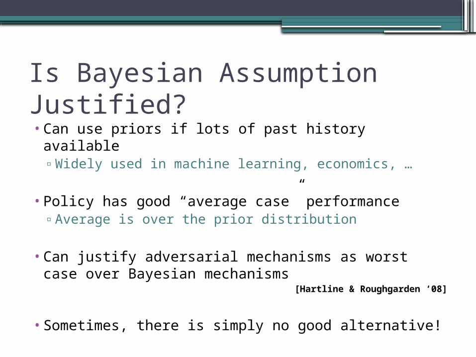
Is Bayesian Assumption Justified?•Can use priors if lots of past history available
▫Widely used in machine learning, economics, …
•Policy has good “average case” performance▫Average is over the prior distribution
•Can justify adversarial mechanisms as worst case over Bayesian mechanisms
[Hartline & Roughgarden ‘08]
•Sometimes, there is simply no good alternative!

Open Questions
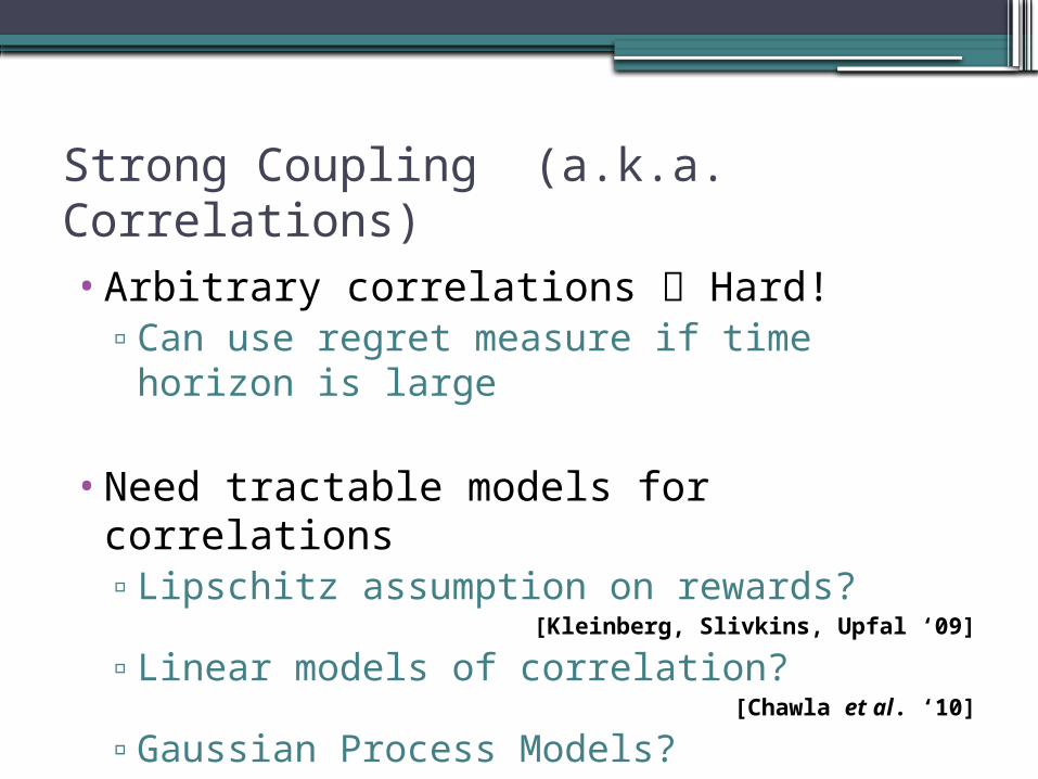
Strong Coupling (a.k.a. Correlations)
•Arbitrary correlations Hard!▫Can use regret measure if time horizon is
large
•Need tractable models for correlations▫Lipschitz assumption on rewards?
[Kleinberg, Slivkins, Upfal ‘09]
▫Linear models of correlation?[Chawla et al. ‘10]
▫Gaussian Process Models?
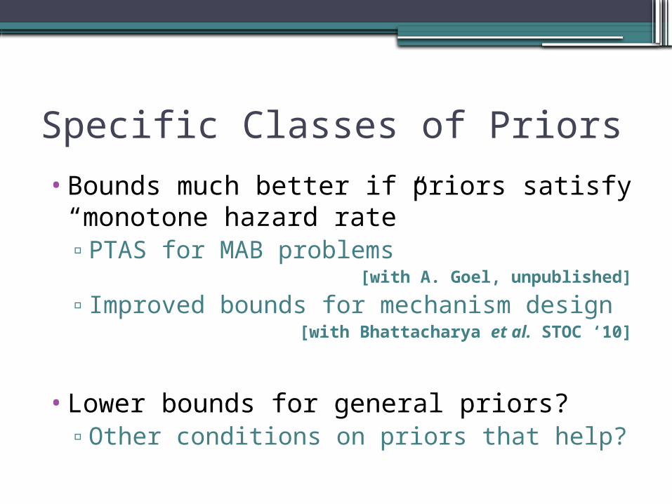
Specific Classes of Priors
•Bounds much better if priors satisfy “monotone hazard rate”▫PTAS for MAB problems
[with A. Goel, unpublished]
▫Improved bounds for mechanism design[with Bhattacharya et al. STOC ‘10]
•Lower bounds for general priors?▫Other conditions on priors that help?
Different Choice of λ
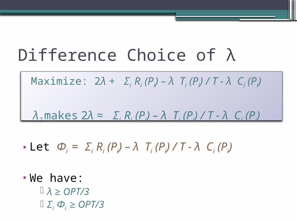
Difference Choice of λ Maximize: 2λ + Σi Ri (Pi) – λ Ti (Pi) / T - λ Ci (Pi)
λ2 makes 2λ ≈ Σi Ri (Pi) – λ Ti (Pi) / T - λ Ci (Pi)
•Let Φi = Σi Ri (Pi) – λ Ti (Pi) / T - λ Ci (Pi)
•We have: λ ≥ OPT/3 Σi Φi ≥ OPT/3
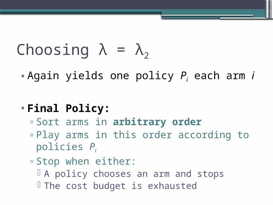
Choosing λ = λ2
•Again yields one policy Pi each arm i
•Final Policy:▫Sort arms in arbitrary order▫Play arms in this order according to
policies Pi
▫Stop when either: A policy chooses an arm and stops The cost budget is exhausted
Accounting the Reward
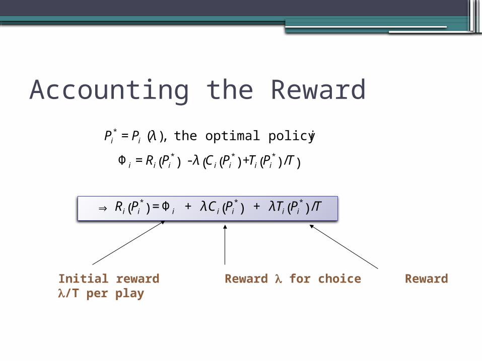
€
Pi* = Pi λ( ), the optimal policy for arm i
Φ i = Ri Pi*
( ) - λ Ci Pi*
( ) +Ti Pi*
( ) /T( )
⇒ Ri Pi*
( ) = Φ i + λCi Pi*
( ) + λTi Pi*
( ) /T
Initial reward Reward for choice Reward /T per play
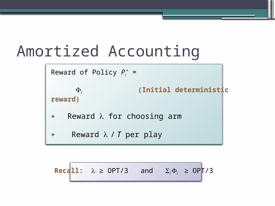
Amortized AccountingReward of Policy Pi
* =
i (Initial deterministic reward)
+ Reward for choosing arm + Reward / T per play
Recall: ≥ OPT/3 and i i ≥ OPT/3
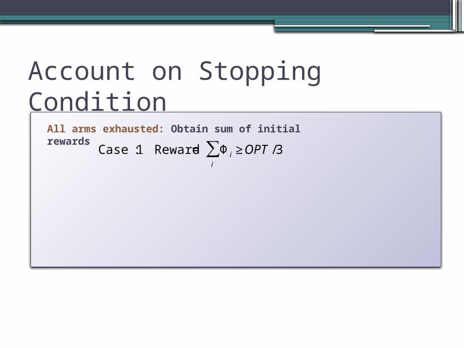
Account on Stopping Condition
€
Case 1: Reward = Φ i ≥ OPT /3i
∑All arms exhausted: Obtain sum of initial rewards
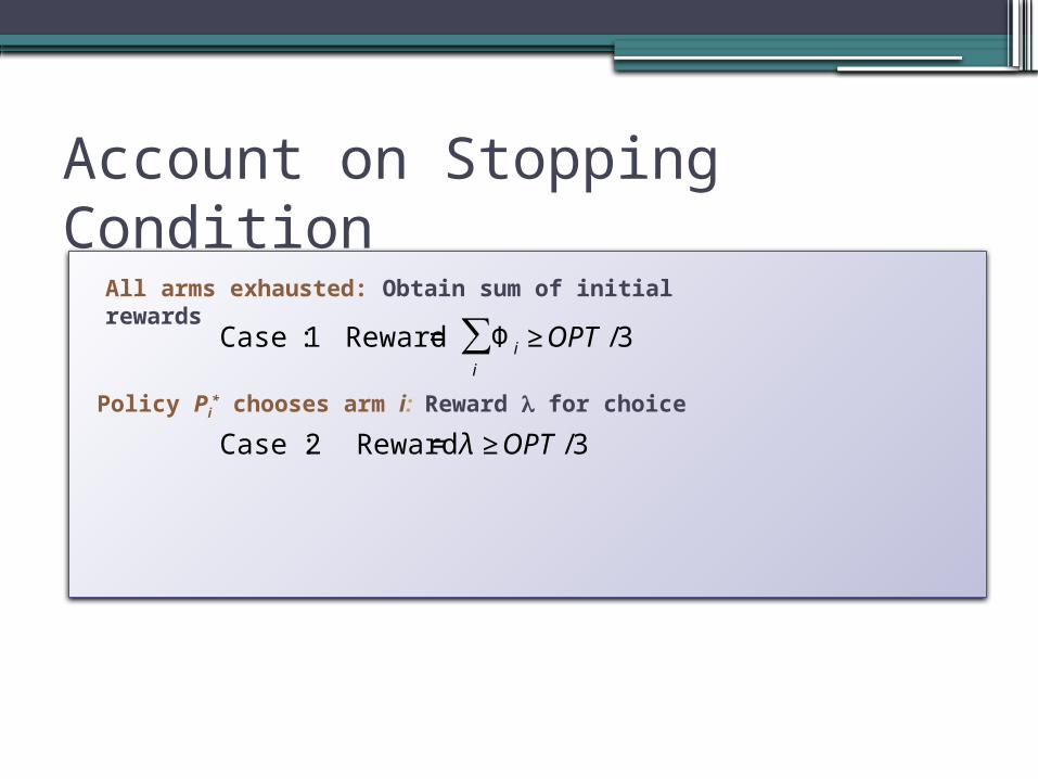
Account on Stopping Condition
€
Case 1: Reward = Φ i ≥ OPT /3i
∑
Case 2 : Reward = λ ≥ OPT /3
All arms exhausted: Obtain sum of initial rewards
Policy Pi* chooses arm i: Reward for choice
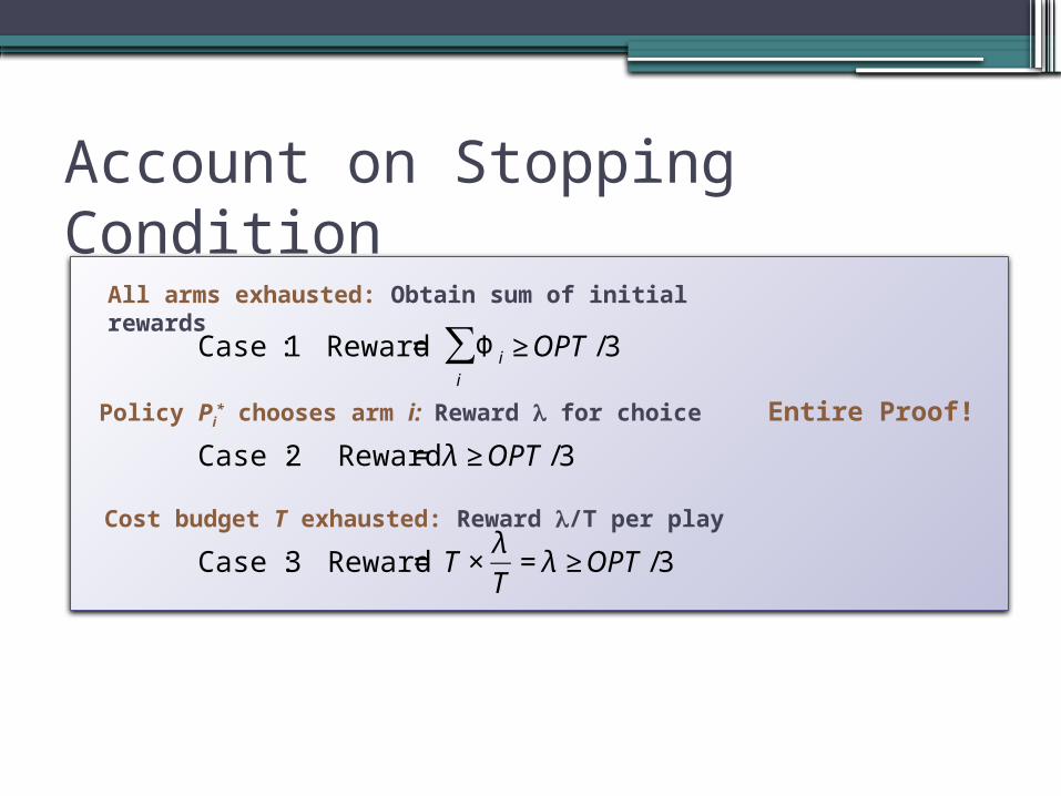
Account on Stopping Condition
€
Case 1: Reward = Φ i ≥ OPT /3i
∑
Case 2 : Reward = λ ≥ OPT /3
Case 3 : Reward = T ×λ
T= λ ≥ OPT /3
All arms exhausted: Obtain sum of initial rewards
Policy Pi* chooses arm i: Reward for choice
Cost budget T exhausted: Reward /T per play
Entire Proof!