This content has been downloaded from IOPscience. Please scroll down to see the full text.

Download details:

IP Address: 138.5.159.110

This content was downloaded on 11/10/2014 at 10:43

Please note that terms and conditions apply.

Weak field black hole formation in asymptotically AdS spacetimes

View the table of contents for this issue, or go to the journal homepage for more

JHEP09(2009)034

(http://iopscience.iop.org/1126-6708/2009/09/034)

Home Search Collections Journals About Contact us My IOPscience

JHEP09(2009)034

Published by IOP Publishing for SISSA

Received: June 5, 2009

Accepted: August 19, 2009

Published: September 4, 2009

Weak field black hole formation in asymptotically AdS

spacetimes

Sayantani Bhattacharyya and Shiraz Minwalla

Department of Theoretical Physics,Tata Institute of Fundamental Research,

Homi Bhabha Rd, Mumbai 400005, India

E-mail: sayanta@theory.tifr.res.in, minwalla@theory.tifr.res.in

Abstract: We use the AdS/CFT correspondence to study the thermalization of a strongly

coupled conformal field theory that is forced out of its vacuum by a source that couples to a

marginal operator. The source is taken to be of small amplitude and finite duration, but is

otherwise an arbitrary function of time. When the field theory lives on Rd−1,1, the source

sets up a translationally invariant wave in the dual gravitational description. This wave

propagates radially inwards in AdSd+1 space and collapses to form a black brane. Outside

its horizon the bulk spacetime for this collapse process may systematically be constructed

in an expansion in the amplitude of the source function, and takes the Vaidya form at

leading order in the source amplitude. This solution is dual to a remarkably rapid and

intriguingly scale dependent thermalization process in the field theory. When the field

theory lives on a sphere the resultant wave either slowly scatters into a thermal gas (dual

to a glueball type phase in the boundary theory) or rapidly collapses into a black hole (dual

to a plasma type phase in the field theory) depending on the time scale and amplitude of

the source function. The transition between these two behaviors is sharp and can be tuned

to the Choptuik scaling solution in Rd,1.

Keywords: Gauge-gravity correspondence, Black Holes in String Theory, AdS-CFT Cor-

respondence

ArXiv ePrint: 0904.0464

c© SISSA 2009 doi:10.1088/1126-6708/2009/09/034

JHEP09(2009)034

Contents

1 Introduction 1

1.1 Translationally invariant asymptotically AdSd+1 collapse 3

1.2 Spherically symmetric collapse in flat space 6

1.3 Spherically symmetric collapse in asymptotically global AdS 7

2 Translationally invariant collapse in AdS 10

2.1 The set up 11

2.2 Structure of the equations of motion 12

2.2.1 Explicit form of the constraints and the dilaton equation 13

2.3 Explicit form of the energy conservation equation 14

2.4 The metric and event horizon at leading order 14

2.5 Formal structure of the expansion in amplitudes 16

2.6 Explicit results for naive perturbation theory to fifth order 17

2.7 The analytic structure of the naive perturbative expansion 19

2.8 Infrared divergences and their cure 19

2.9 The metric to leading order at all times 21

2.10 Resummed versus naive perturbation theory 21

2.11 Resummed perturbation theory at third order 22

3 Spherically symmetric asymptotically flat collapse 24

3.1 The set up 24

3.2 Regular amplitude expansion 26

3.2.1 Regularity implies energy conservation 27

3.3 Leading order metric and event horizon for black hole formation 28

3.4 Amplitude expansion for black hole formation 29

3.5 Analytic structure of the naive perturbation expansion 30

3.6 Resummed perturbation theory at third order 31

4 Spherically symmetric collapse in global AdS 33

4.1 Set up and equations 34

4.2 Regular small amplitude expansion 35

4.3 Spacetime and event horizon for black hole formation 37

4.4 Amplitude expansion for black hole formation 38

4.5 Explicit results for naive perturbation theory 39

4.6 The solution at late times 41

5 Discussion 41

JHEP09(2009)034

A Translationally invariant graviton collapse 44

A.1 The set up and summary of results 45

A.2 The energy conservation equation 46

A.3 Structure of the amplitude expansion 47

A.4 Explicit results up to 5th order 48

A.5 Late times resummed perturbation theory 49

B Generalization to arbitrary dimension 50

B.1 Translationally invariant scalar collapse in arbitrary dimension 50

B.1.1 Odd d 50

B.1.2 Even d 53

B.2 Spherically symmetric flat space collapse in arbitrary dimension 58

B.2.1 Odd d 58

B.2.2 Even d 59

B.3 Spherically symmetric asymptotically AdS collapse in arbitrary dimension 60

1 Introduction

The AdS/CFT correspondence identifies asymptotically AdS gravitational dynamics with

the master field evolution of ‘large N ’ field theories. In particular, it relates the evolution

of spacetimes with horizons to the non equilibrium statistical dynamics of the high temper-

ature phase of the dual field theory. This connection has recently been studied in detail in

a near equilibrium limit. It has been established that the spacetimes that locally (i.e. tube

wise) approximate the black brane metric obey the equations of boundary fluid dynamics

with gravitationally determined dissipative constants.1 The equations of fluid dynamics

are thus embedded in a long distance sector of asymptotically AdS gravity, a fascinating

connection that promises to prove useful in many ways.

Given the success in using gravitational physics to study near equilibrium field the-

ory dynamics, it is natural to attempt to use gravitational dynamics to study far from

equilibrium field theory processes. In this paper we will study the gravitational dual of

the process of equilibration; i.e the dynamical passage of a system from a pure state in

its ‘low temperature’ phase to an approximately thermalized state in its high temperature

phase (see [35–48] for closely related earlier work and [49–52] for analyses of thermalization

directly in large N gauge theories). As has been remarked by several authors, this process

is dual to the gravitational process of black hole formation via gravitational collapse. The

dynamical process is fascinating in its own right, but gains additional interest in asymptot-

ically AdS spaces because of its link to field theory equilibration dynamics. In this paper

we study asymptotically AdS (and briefly asymptotically flat) collapse processes in a weak

field limit that displays rich dynamics while allowing for analytic control.

1See [1–20] for a recent structural understanding of this connection. See the reviews [21–23]for references

to important earlier work. See also [24–34] for related line of development.

– 1 –

JHEP09(2009)034

Vacuum AdS

SingularityEvent

Horizon

CollapsingShell

Metric

BlackBrane

Figure 1. Cross section of the causal diagram for the collapse process in an asymptotically global

AdSd+1 space. The conventional Penrose diagram for this process would include only the half of

the diagram that to the right of its vertical axis of symmetry

An AdS collapse process that could result in black hole formation may be set up,

following Yaffe and Chesler [53], as follows . Consider an asymptotically locally AdS

spacetime, and let R denote a finite patch of the conformal boundary of this spacetime.

We choose our spacetime to be exactly AdS outside the causal future of R. On R we turn

on the non normalizable part of a massless bulk field. This boundary condition sets up

an ingoing shell of the corresponding field that collapses in AdS space. Under appropriate

conditions the subsequent dynamics can result in black hole formation.

In this paper we will study the AdS collapse scenario (plus a flat space counterpart)

outlined in the previous paragraph in a weak field limit; i.e. we always choose the amplitude

ǫ of the non normalizable perturbation to be small. In the interest of simplicity we also

focus on situations that preserve a great deal of symmetry, as we explain further below. In

the rest of this introduction we describe the three classes of collapse situations we study,

and the principal results of our analysis.2

2In most of the bulk of the text of this paper we only present formulae for asymptotically AdSd+1

spacetimes for the smallest nontrivial value of d namely d = 3. As we explain in the appendix B however,

most of the qualitative results of our analysis apply to arbitrary odd d for d ≥ 3 and also plausibly to

arbitrary even d for d ≥ 4.

– 2 –

JHEP09(2009)034

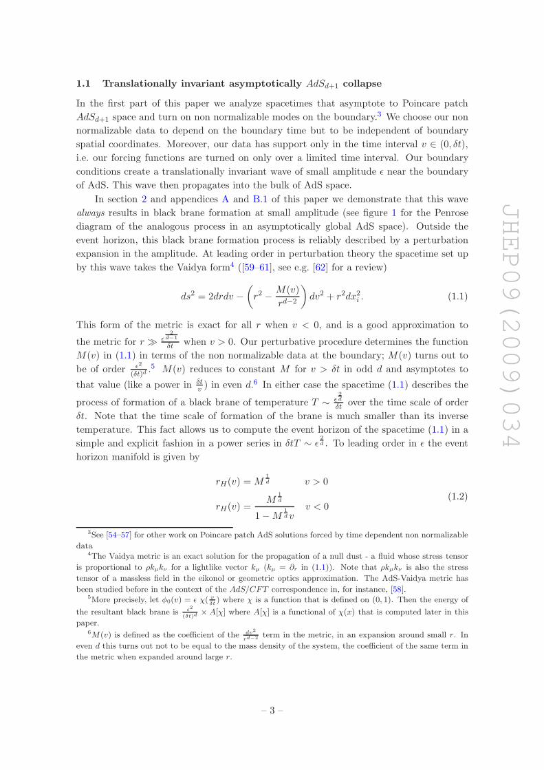
1.1 Translationally invariant asymptotically AdSd+1 collapse

In the first part of this paper we analyze spacetimes that asymptote to Poincare patch

AdSd+1 space and turn on non normalizable modes on the boundary.3 We choose our non

normalizable data to depend on the boundary time but to be independent of boundary

spatial coordinates. Moreover, our data has support only in the time interval v ∈ (0, δt),

i.e. our forcing functions are turned on only over a limited time interval. Our boundary

conditions create a translationally invariant wave of small amplitude ǫ near the boundary

of AdS. This wave then propagates into the bulk of AdS space.

In section 2 and appendices A and B.1 of this paper we demonstrate that this wave

always results in black brane formation at small amplitude (see figure 1 for the Penrose

diagram of the analogous process in an asymptotically global AdS space). Outside the

event horizon, this black brane formation process is reliably described by a perturbation

expansion in the amplitude. At leading order in perturbation theory the spacetime set up

by this wave takes the Vaidya form4 ([59–61], see e.g. [62] for a review)

ds2 = 2drdv −(

r2 − M(v)

rd−2

)

dv2 + r2dx2i . (1.1)

This form of the metric is exact for all r when v < 0, and is a good approximation to

the metric for r ≫ ǫ2

d−1

δtwhen v > 0. Our perturbative procedure determines the function

M(v) in (1.1) in terms of the non normalizable data at the boundary; M(v) turns out to

be of order ǫ2

(δt)d .5 M(v) reduces to constant M for v > δt in odd d and asymptotes to

that value (like a power in δtv) in even d.6 In either case the spacetime (1.1) describes the

process of formation of a black brane of temperature T ∼ ǫ2d

δtover the time scale of order

δt. Note that the time scale of formation of the brane is much smaller than its inverse

temperature. This fact allows us to compute the event horizon of the spacetime (1.1) in a

simple and explicit fashion in a power series in δtT ∼ ǫ2d . To leading order in ǫ the event

horizon manifold is given by

rH(v) = M1d v > 0

rH(v) =M

1d

1 −M1d v

v < 0(1.2)

3See [54–57] for other work on Poincare patch AdS solutions forced by time dependent non normalizable

data4The Vaidya metric is an exact solution for the propagation of a null dust - a fluid whose stress tensor

is proportional to ρkµkν for a lightlike vector kµ (kµ = ∂r in (1.1)). Note that ρkµkν is also the stress

tensor of a massless field in the eikonol or geometric optics approximation. The AdS-Vaidya metric has

been studied before in the context of the AdS/CFT correspondence in, for instance, [58].5More precisely, let φ0(v) = ǫ χ( v

δt) where χ is a function that is defined on (0, 1). Then the energy of

the resultant black brane is ǫ2

(δt)d× A[χ] where A[χ] is a functional of χ(x) that is computed later in this

paper.6M(v) is defined as the coefficient of the dv2

rd−2term in the metric, in an expansion around small r. In

even d this turns out not to be equal to the mass density of the system, the coefficient of the same term in

the metric when expanded around large r.

– 3 –

JHEP09(2009)034

All of the spacetime outside the event horizon (1.2) lies within the domain of validity of

our perturbative procedure. Of course perturbation theory does not accurately describe

the process of singularity formation of the black brane. However the region where pertur-

bation theory breaks down (and so (1.1) is not reliable) is contained entirely within the

event horizon of (1.1). Consequently, the region outside perturbative control is causally

disconnected from physics outside the event horizon, so our perturbation procedure gives a

fully reliable description of the dynamics outside the event horizon. It follows in particular

that any singularities that develop in our solution are is always shielded by a regular event

horizon, in agreement with the cosmic censorship conjecture.7

In section 2 we demonstrate that the corrections to the Vaidya metric (1.1) may be

systematically computed in a power series in positive fractional powers of ǫ. At any order in

the perturbation expansion, the metric may be determined analytically for times v ≪ T−1

(T is the temperature of the eventually formed brane). At times of order or larger than

T−1, perturbative corrections to the metric are determined in terms solutions of univer-

sal(i.e. independent of the form of the perturbation) linear differential equations which we

have only been able to solve numerically. Even at late times, however our perturbative

procedure analytically determines the dependence of observables on the functional form of

the non normalizable perturbation, allowing us to draw conclusions that are valid for small

amplitude perturbation of arbitrary form.

Let us now word our results in dual field theoretic terms. Our gravity solution describes

a CFT initially in its vacuum state. Over the time period (0, δt) the field theory is per-

turbed by a translationally invariant time dependent source, of amplitude ǫ, that couples

to a marginal operator. This coupling pumps energy into this system. Our perturbative

gravitational solution gives a detailed description of the subsequent equilibration process;

in particular it gives a precise formula for the temperature of the final equilibrium configu-

ration as a function of the perturbation function. It also, very surprisingly, asserts that for

some purposes8 our system appears to thermalize almost instanteneously at leading order

in ǫ. We pause to explain this in detail.9

A field theorist presented with a flow towards equilibrium might choose to probe this

flow by perturbing it with an infinitesimal source, localized at some time. He would then

measure the subsequent change in the solution in response to this perturbation. However

note that the spacetime in (1.1) is identical to the spacetime outside a static uniform black

brane for v > δt when d is odd (and for v ≫ δt for even d). It follows that the response of

our system to any boundary perturbation localized at times v > δt in odd d (and at v ≫ δt

in even d) will be identical to the response of a thermally equilibrated system to the same

perturbation. In other words our system responds to perturbations at v > δt as if it had

equilibrated instanteneously.

A field theorist could also characterize a flow towards equilibrium by recording the

7We thank M. Rangamani for discussions on this point.8In particular, in even bulk space time dimensions, one point functions of all local operators reduce to

their thermal values as soon as the perturbation is switched off. While thermalization of one point functions

is not instantaneous in odd bulk space times it appears to take place over a time scale of order δt.9The rest of this subsection was worked out in collaboration with O. Aharony, B. Kol and S. Raju. See

also the paper [48], by Lin and Shuryak, for a very similar earlier discussion. We thank E. Shuryak for

bringing this paper to our attention.

– 4 –

JHEP09(2009)034

values of all observables as a function of time (in the absence of any further perturbation).

The full set of observables consists of expectation values of the arbitrary product of ‘gauge

invariant’ operators, i.e. quantities that in a gauge theory would take the form

〈TrO1TrO2 . . . T rOn〉.

In this paper we work in the strict large N limit (i.e. the strictly classical limit from the dual

bulk viewpoint). In this limit trace factorization (or the classical nature of the dual bulk

theory) ensures that the expectation value of products equals the product of expectation

values. In other words our set of observables is given precisely by the one point functions

of all gauge invariant operators.

Now note that expectation values of all local boundary operators are determined by

the bulk solution in a neighborhood of the boundary values. As the metric (1.1) is identical

to the metric of a uniform black brane in the neighbourhood of the boundary when v > δt,

it follows that the expectation value of all local boundary operators reduce instantaneously

to their thermal values in odd d (and when v ≫ δt in even d). Consequently, all local

operators appear to thermalize instanteneously.

Not all gauge invariant operators are local, however. A field theorist could also record

the values of non local observables, like circular Wilson Loops of radius a, as a function

of time. As nonlocal observables probe the spacetime away from the boundary, their

expectation values reduce to thermal results only after a larger time that depends on

the size of the loop (this time is proportional to a at small a). So a diligent infinite N

field theorist would be able to distinguish (1.1) from absolute thermal equilibrium at times

greater than δt, but only by keeping track of the expectation values of non local observables.

If one were to retreat away from the large N limit one would find large new classes of

gauge invariant observables; the connected correlators of, for instance, local gauge invariant

operators. Such correlators also sample spacetime away from the boundary, the distance

scale of this nonlocal sampling being set by the separation between the operator insertions

(see [58] for a detailed discussion of properties of correlation functions in asymptotically

AdS Vaidya type metrics). As in our discussion of Wilson loops above, the time scale for

thermalization of such connected correlators is set by their separation (it is proportional

to their separation when this separation is small).

As we have seen, the time scale of equlibration of the solutions described in this paper

depend on the precise question you ask about it. We would now like to describe a concrete

and possibly practically important experimental sense in which our system behaves as if it

were instanteneously thermally equilibrated.

Consider the response of a CFT in its vacuum to a forcing function that varies —

though only slowly — with ~x. We anticipate that at v = δt the corresponding spacetime is

locally (tube wise) well described by a black brane metric with a value of the temprature

that varies with ~x (see (5.1) and the discusson arounf it in section 5). According to [1–20],

the subsequent evolution of our system is governed by the equations of boundary fluid

dynamics. The initial conditions for the relevant fluid flow are given at v = δt. Conse-

quently an experimentalist who observes the subsequent fluid flow, and back calculates,

would conclude that his system was thermalized at v = δt.

– 5 –

JHEP09(2009)034

The thought experiment of the previous paragraph is reminiscent of situation at the

RHIC experiment. The back calculation described in this paragraph, in the context of

that experiment, suggests that the RHIC system is governed by fluid dynamics at times

of order 0.5 fermi after the collision, much faster than suggested by naive estimates for

thermalization time (see [63] and references therein). It is natural to wonder whether the

mechanisims for rapid equilibration of this paper have qualitative applicability to the RHIC

experiment. We leave a serious investigation of this question to future work.

In summary, (1.1) describes a system whose response to additional external pertur-

bations at v > δt is identical to that of a thermally equilibrated system and whose one

point functions of local operators also instanteneously thermalize. However expectation

values of non local observables (or correlators) thermalize more slowly, over a time scale

that depends on the smearing size of the observable (or correlator). We find instantenous

thermalization of expectation values local operators and the scale dependence in the pro-

cess of equilibration fascinating. In fact this discussion is reminiscent of precursors in the

AdS/CFT correspondence [64–67].

We emphasize that our discussion of thermalization applies only at leading order in ǫ

expansion. Indeed our analysis was based on (1.1) which accurately describes our spacetime

only at leading order in ǫ. At sub leading orders (1.1) is corrected by perturbations that

decay to the black brane result only over the time scale 1/T , in accordance with naive

expextation. Consequently, the instantaneous thermalization of expectation values of local

operators is corrected by sub leading equilibration process that take place over the time

scale 1/T , the thermalization of linear fluctuations about a brane of temperature T . Note,

in particular, that we have no reason so suspect that thermalization occurs over a time

period that is faster than the naive estimate v = 1T

when ǫ is of order unity or larger.

1.2 Spherically symmetric collapse in flat space

We next turn to the perturbative study of spherically symmetric collapse in an asymptoti-

cally flat space. Consider a spherically symmetric shell, propagating inwards, focused onto

the origin of an asymptotically flat space. Such a shell may qualitatively be characterized

by its thickness and mass, or (more usefully for our purposes) by the Schwarzschild radius

rH associated with this mass. It is a well appreciated fact that this collapse process may

reliably be described in an amplitude expansion when y ≡ rHδt

is very small. The starting

point for this expansion is the propagation of a free scalar shell. This free motion receives

weak scattering corrections at small y, which may be computed perturbatively.

In section 3 of this paper we demonstrate that this flat space collapse process may also

be reliably described in an amplitude expansion at large y. In section 3 and appendix B.2

we study this collapse process mainly in odd d (i.e. in even bulk spacetime dimensions). The

starting point for this expansion is a Vaidya metric similar to (1.1), whose event horizon

we are able to reliably compute in a power series expansion in inverse powers of y. Outside

this event horizon the dilaton is everywhere small and the Vaidya metric receives only weak

scattering corrections that it may systematically be computed in a power series in 1y

at

large y. As in the previous subsection, our perturbative procedure is not valid everywhere;

– 6 –

JHEP09(2009)034

however the breakdown of perturbation theory occurs entirely within the event horizon,

and so does not impinge on our control of the solution outside the event horizon.

At early times we are able to determine the perturbative corrections to the metric

(order by order in 1y) in an entirely analytic manner. However late time corrections to

the metric are computed in terms of the solutions to relevant universal linear differential

equations, which we have not been able to solve analytically. However our perturbative

solutions carry a considerable amount of information, even in the absence of an explicit

analytic solution to the relevant differential equation. As an example, in section 3 we de-

termine the fraction of energy of the incident pulse that is radiated back out to infinity

to nontrivial leading order in the expansion in 1y. We are able to analytically determine

the dependence of this fraction on the shape of the incident pulse upto an overall con-

stant (see (3.34)). The determination of the value of this constant requires knowledge of

the explicit solution of the ‘universal’ differential equation listed in section 3, and may

presumably be determined numerically.

An order parameter (the presence of an event horizon at late times) distinguishes small

y from large y behavior, so the transition between them must be sharp. This observation

was originally made about twenty years ago in classic paper by Christodoulou (see [68])

and references therein) who rigorously demonstrated that collapse at arbitrarily large y

results in black hole formation, while collapse at small y does not. As the fascinating

transition between small and large y behaviors (which has been extensively in a programme

of numerical relativity initiated by Choptuik [69])10 presumably occurs at y of order unity.

Consequently it cannot be studied in either the small y or the large y expansions described

in our paper.

As we do not have a holographic description of gravitational dynamics in an asymp-

totically flat space, we are unable to give a direct dual field theoretic interpretation of our

results reviewed in this subsection. See however, the next subsection.

1.3 Spherically symmetric collapse in asymptotically global AdS

The process of spherically symmetric collapse in an asymptotically global AdS space consti-

tutes an interesting one parameter interpolation between the collapse processes described

in subsections 1.1 and 1.2. We study such collapse processes in section 4 of this paper. In

section 4 we have studied this collapse situation in detail only in d = 3. In this subsec-

tion we report the generalization of these results to arbitrary odd dimension, which may

qualitatively be inferred from the results of appendix B.

Consider a global AdS space, whose boundary is taken to be a sphere of radius R

× time. Consider a collapse process initiated by radially symmetric non normalizable

boundary conditions that are turned on, uniformly over the boundary sphere, over a time

interval δt. The amplitude ǫ of this perturbation together with the dimensionless ratio

x ≡ δtR

, constitute the two qualitatively important parameters of this perturbation. In the

limit x→ 0 it is obvious that the collapse process of this subsection effectively reduces to

10See [70, 71] for reviews and [72–77] for recent work interpreting this transition in the context of the

AdS/CFT correspondence.

– 7 –

JHEP09(2009)034

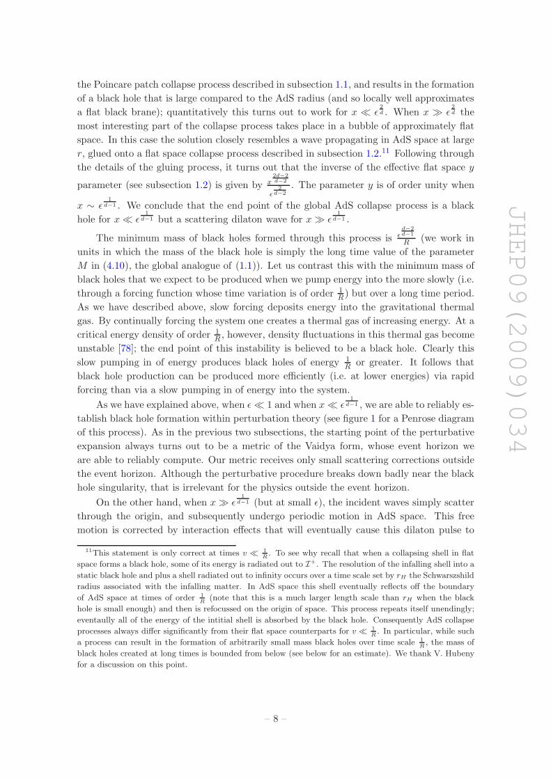
the Poincare patch collapse process described in subsection 1.1, and results in the formation

of a black hole that is large compared to the AdS radius (and so locally well approximates

a flat black brane); quantitatively this turns out to work for x ≪ ǫ2d . When x ≫ ǫ

2d the

most interesting part of the collapse process takes place in a bubble of approximately flat

space. In this case the solution closely resembles a wave propagating in AdS space at large

r, glued onto a flat space collapse process described in subsection 1.2.11 Following through

the details of the gluing process, it turns out that the inverse of the effective flat space y

parameter (see subsection 1.2) is given by x2d−2d−2

ǫ2

d−2. The parameter y is of order unity when

x ∼ ǫ1

d−1 . We conclude that the end point of the global AdS collapse process is a black

hole for x≪ ǫ1

d−1 but a scattering dilaton wave for x≫ ǫ1

d−1 .

The minimum mass of black holes formed through this process is ǫd−2d−1

R(we work in

units in which the mass of the black hole is simply the long time value of the parameter

M in (4.10), the global analogue of (1.1)). Let us contrast this with the minimum mass of

black holes that we expect to be produced when we pump energy into the more slowly (i.e.

through a forcing function whose time variation is of order 1R

) but over a long time period.

As we have described above, slow forcing deposits energy into the gravitational thermal

gas. By continually forcing the system one creates a thermal gas of increasing energy. At a

critical energy density of order 1R

, however, density fluctuations in this thermal gas become

unstable [78]; the end point of this instability is believed to be a black hole. Clearly this

slow pumping in of energy produces black holes of energy 1R

or greater. It follows that

black hole production can be produced more efficiently (i.e. at lower energies) via rapid

forcing than via a slow pumping in of energy into the system.

As we have explained above, when ǫ≪ 1 and when x≪ ǫ1

d−1 , we are able to reliably es-

tablish black hole formation within perturbation theory (see figure 1 for a Penrose diagram

of this process). As in the previous two subsections, the starting point of the perturbative

expansion always turns out to be a metric of the Vaidya form, whose event horizon we

are able to reliably compute. Our metric receives only small scattering corrections outside

the event horizon. Although the perturbative procedure breaks down badly near the black

hole singularity, that is irrelevant for the physics outside the event horizon.

On the other hand, when x≫ ǫ1

d−1 (but at small ǫ), the incident waves simply scatter

through the origin, and subsequently undergo periodic motion in AdS space. This free

motion is corrected by interaction effects that will eventually cause this dilaton pulse to

11This statement is only correct at times v ≪ 1R

. To see why recall that when a collapsing shell in flat

space forms a black hole, some of its energy is radiated out to I+. The resolution of the infalling shell into a

static black hole and plus a shell radiated out to infinity occurs over a time scale set by rH the Schwarszshild

radius associated with the infalling matter. In AdS space this shell eventually reflects off the boundary

of AdS space at times of order 1R

(note that this is a much larger length scale than rH when the black

hole is small enough) and then is refocussed on the origin of space. This process repeats itself unendingly;

eventaully all of the energy of the intitial shell is absorbed by the black hole. Consequently AdS collapse

processes always differ significantly from their flat space counterparts for v ≪ 1R

. In particular, while such

a process can result in the formation of arbitrarily small mass black holes over time scale 1R

, the mass of

black holes created at long times is bounded from below (see below for an estimate). We thank V. Hubeny

for a discussion on this point.

– 8 –

JHEP09(2009)034

x

Amplitude (epsilon)

Large Black Hole

Small Black

Hole

Thermal Gas

Figure 2. The ‘Phase Diagram’ for our dynamical stirring in global AdS. The final outcome is a

large black hole for x≪ ǫ2

d (below the dashed curve), a small black hole for x≪ ǫ1

d−1 (between the

solid and dashed curve) and a thermal gas for x ≫ ǫ1

d−1 . The solid curve represents non analytic

behaviour (a phase transition) while the dashed curve is a crossover.

deviate significantly from its free motion over a time scale that we expect to scale like a

positive power of x2d−2d−2

ǫ2

d−2times the inverse radius of the sphere.12

Let us now reword our results in field theory terms. Any CFT that admits a two

derivative gravity dual description undergoes a first order finite temperature phase tran-

sition when studied on Sd−1. The low temperature phase is a gas of ’glueballs’ (dual to

gravitons) while the high temperature phase is a strongly interacting, dissipative, ‘plasma’

(dual to the black hole). The gravitational solutions of this paper describe such a CFT on

a sphere, initially in its vacuum state. We then excite the CFT over a time δt by turning on

a spherically symmetric source function that couples to a marginal operator. The most im-

portant qualitative question about the subsequent equilibration process is: in which phase

does the system eventually settle down within classical dynamics (i.e. ignoring tunneling

effects) ? Our gravitational solutions predict that the system settles in its free particle

phase when x ≫ ǫ1

d−1 but in the plasma phase when x ≪ ǫ1

d−1 . As in subsection 1.1 the

equilibration in the high temperature phase is almost instantaneous. However equilibration

in the low temperature phase appears to occur over a much longer time scale. We note

also that the transition between these two end points appears to be singular (this is the

Choptuik singularity) in the large N limit.13 This singularity is presumably smoothed out

by fluctuations at finite N , a phenomenon that should be dual to the smoothing out of a

naked gravitational singularity by quantum gravity fluctuations.

12We expect this pulse to thermalize over an even longer time scale, one that scales as a positive power

of the larger number, xd

ǫ2.

13See section 5 for a discussion of the effects of potential Gregory-Laflamme type instabilities near this

singular surface.

– 9 –

JHEP09(2009)034

In the rest of this paper and in the appendices we will present a detailed study of the

collapse scenarios outlined in this introduction. In the last section of this paper we also

present a discussion of our results.

2 Translationally invariant collapse in AdS

In this section we study asymptotically planar (Poincare patch) AdSd+1 solutions to nega-

tive cosmological constant Einstein gravity interacting with a minimally coupled massless

scalar field (note that this system obeys the null energy condition). We focus on solutions

in which the boundary value of the scalar field takes a given functional form φ0(v) in the

interval (0, δt) but vanishes otherwise. The amplitude of φ0(v) (which we schematically

refer to as ǫ below) will be taken to be small in most of this section. The boundary dual

to our setup is a d dimensional conformal field theory on Rd−1,1, perturbed by a spatially

homogeneous and isotropic source function, φ0(v), multiplying a marginal scalar operator.

Note that our boundary conditions preserve an Rd−1 ×SO(d− 1) symmetry (the Rd−1

factor is boundary spatial translations while the SO(d− 1) is boundary spatial rotations).

In this section we study solutions on which Rd−1⋊ SO(d − 1) lifts to an isometry of the

full bulk spacetime. In other words the spacetimes studied in this section preserve the

maximal symmetry allowed by our boundary conditions. As a consequence all bulk fields

in our problem are functions of only two variables; a radial coordinate r and an Eddington

Finkelstein ingoing time coordinate v. The chief results of this section are as follows:

• The boundary conditions described above result in black brane formation for an

arbitrary (small amplitude) source functions φ0(v).

• Outside the event horizon of our spacetime, we find an explicit analytic form for

the metric as a function of φ0(v). Our metric is accurate at leading order in the ǫ

expansion, and takes the Vaidya form (1.1) with a mass function that we determine

explicitly as a function of time.

• In particular, we find that the energy density of the resultant black brane is given,

to leading order, by

C2 =2d−1

(d− 1)

(

(d−12 )!

(d− 1)!

)2∫ ∞

−∞

(

(

∂d+12

t φ0(t)

)2)

(2.1)

in odd d and by

C2 = − d2

(d− 1)2d1

(

d2 !)2

∫

dt1dt2∂d+22

t1φ0(t1) ln(t1 − t2)θ(t1 − t2)∂

d+22

t2φ0(t2) (2.2)

in even d. Note that, in each case, C2 ∼ ǫ2

(δt)d .

• We find an explicit expression for the event horizon of the resultant solutions, at

leading order, and thereby demonstrate that singularities formed in the process of

black brane formation are always shielded by a regular event horizon at small ǫ.

– 10 –

JHEP09(2009)034

• Perturbation theory in the amplitude ǫ yields systematic corrections to this leading

order metric. We unravel the structure of this perturbation expansion in detail and

compute the first corrections to the leading order result.

While every two derivative theory of gravity that admits an AdS solutions admits a

consistent truncation to Einstein gravity with a negative cosmological constant, the same

statement is clearly not true of gravity coupled to a minimally coupled massless scalar field.

It is consequently of considerable interest to note that results closely analogous to those

described above also apply to the study of Einstein gravity with a negative cosmological

constant. In appendix A we analyze the process of black brane formation by gravitational

wave collapse in the theory of pure gravity (similar to the set up of [53]), and find results

that are qualitatively very similar to those reported in this section. The solutions of

appendix A yield the dual description of a class of thermalization processes in every 3

dimensional conformal field theory that admits a dual description as a two derivative

theory of gravity. In fact, the close similarity of the results of appendix A with those

of this section, lead us to believe that the results reported in this section are qualitatively

robust. In particular we think it is very likely that results of this section will qualitatively

apply to the most general small amplitude translationally invariant collapse process in the

systems we study.

2.1 The set up

Consider a minimally coupled massless scalar (the ‘dilaton’) interacting with negative cos-

mological constant Einstein gravity in d+ 1 spacetime dimensions

S =

∫

dd+1x√g

(

R− d(d− 1)

2− 1

2(∂φ)2

)

(2.3)

The equations of motion that follow from the Lagrangian (2.3) are

Eµν ≡ Gµν −1

2∂µφ∂νφ+ gµν

(

−d(d− 1)

2+

1

4(∂φ)2

)

= 0

∇2φ = 0

(2.4)

where the indices µ, ν range over all d+ 1 spacetime coordinates. As mentioned above, in

this section we are interested in locally asymptotically AdSd+1 solutions to these equations

that preserve an Rd−1 × SO(d − 1) symmetry group. This symmetry requirement forces

the boundary metric to be Weyl flat (i.e. Weyl equivalent to flat Rd−1,1); however it allows

the boundary value of the scalar field to be an arbitrary function of boundary time v. We

choose this function as

φ0(v) = 0 (v < 0)

φ0(v) < ǫ (0 < v < δt)

φ0(v) = 0 (v > δt)

(2.5)

(we also require that φ0(v) and its first few derivatives are everywhere continuous.14).

14We expect that all our main physical conclusions will continue to apply if we replace our φ0 — which

is chosen to strictly vanish outside (0, δt) — by any function that decays sufficiently rapidly outside this

range.

– 11 –

JHEP09(2009)034

Everywhere in this paper we adopt the ‘Eddington Finkelstein’ gauge grr = gri = 0

and grv = 1. In this gauge, and subject to our symmetry requirement, our spacetime takes

the form

ds2 = 2drdv − g(r, v)dv2 + f2(r, v)dx2i

φ = φ(r, v).(2.6)

The mathematical problem we address in this subsection is to solve the equations of

motion (2.4) for the functions φ, f and g, subject to the pure AdS initial conditions

g(r, v) = r2 (v < 0)

f(r, v) = r (v < 0)

φ(r, v) = 0 (v < 0)

(2.7)

and the large r boundary conditions

limr→∞

g(r, v)

r2= 1

limr→∞

f(r, v)

r= 1

limr→∞

φ(r, v) = φ0(v)

(2.8)

The Eddington Finkelstein gauge we adopt in this paper does not completely fix gauge

redundancy (see [53] for a related observation). The coordinate redefinition r = r + h(v)

respects both our gauge choice as well as our boundary conditions. In order to completely

define the mathematical problem of this section, we must fix this ambiguity. We have

assumed above that f(r, v) = r + O(1) at large r. It follows that under the unfixed

diffeomorphism, f(r, v) → f(r, v) + h(v) + O(1/r). Consequently we can fix this gauge

redundancy by demanding that f(r, v) ≈ r + O(1/r) at large r. We make this choice in

what follows. As we will see below, it then follows from the equations of motion that

g(r) = r2 + O(1). Consequently, the boundary conditions (2.8) on the fields g, f and φ,

may be restated in more detail as

g(r, v) = r2(

1 + O(

1

r2

))

f(r, v) = r

(

1 + O(

1

r2

))

φ(r, v) = φ0(v) + O(

1

r

)

(2.9)

Equations (2.4), (2.6), (2.7) and (2.9) together constitute a completely well defined dy-

namical system. Given a particular forcing function φ0(v), these equations and boundary

conditions uniquely determine the functions φ(r, v), g(r, v) and f(r, v).

2.2 Structure of the equations of motion

The nonzero equations of motion (2.4) consist of four nontrivial Einstein equations Err,

Erv, Evv and∑

iEii (where the index i runs over the d − 1 spatial directions) together

– 12 –

JHEP09(2009)034

with the dilaton equation of motion. For the considerations that follow below, we will find

it convenient to study the following linear combinations of equations

E1c = gvµEµr

E2c = gvµEµv

Eec = grµEµr

Ed =

d−1∑

i=1

Eii

Eφ = ∇2φ

(2.10)

Note that the equations E1c and E2

c are constraint equations from the point of view of

v evolution.

It is possible to show that Ed and d(rEec)dr

both automatically vanish whenever E1c =

E2c = Eφ = 0. This implies that this last set of three independent equations — supple-

mented by the condition that rEec = 0 at any one value of r — completely exhaust the

dynamical content of (2.4). As a consequence, in the rest of this paper we will only bother

to solve the two constraint equations and the dilaton equation, but take care to simulta-

neously ensure that rEec = 0 at some value of r. It will often prove useful to impose the

last equation at arbitrarily large r. This choice makes the physical content of rEec = 0

manifest; this is simply the equation of energy conservation in our system.15

2.2.1 Explicit form of the constraints and the dilaton equation

With our choice of gauge and notation the dilaton equation takes the minimally cou-

pled form

∂r

(

fd−1g∂rφ)

+ ∂v

(

fd−1∂rφ)

+ ∂r

(

fd−1∂vφ)

= 0 (2.11)

Appropriate linear combinations of the two constraint equations take the form

(∂rφ)2 = −2(d− 1)∂2r f

f

∂r

(

fd−2g∂rf + 2fd−2∂vf)

= fd−1d

(2.12)

Note that the equations (2.12) (together with boundary conditions and the energy

conservation equation) permit the unique determination of f(r, v0) and g(r, v0) in terms

of φ(r, v0) and φ(r, v0) (where v0 is any particular time). It follows that f and g are not

independent fields. A solution to the differential equation set (2.11) and (2.12) is completely

specified by the value of φ on a constant v slice (note that the equations are all first order

in time derivatives, so φ on the slice is not part of the data of the problem) together with

the boundary condition φ0(v).

15It turns out that both Ed and the dilaton equation of motion are automatically satisfied whenever Eec

together with the two Einstein constraint equations are satisfied. Consequently Eec plus the two Einstein

constraint equations form another set of independent equations. This choice of equations has the advantage

that it does not require the addition of any additional condition analogous to energy conservation. However

it turns out to be an inconvenient choice for implementing the ǫ expansion of this paper, and we do not

adopt it in this paper.

– 13 –

JHEP09(2009)034

2.3 Explicit form of the energy conservation equation

In this section we give an explicit form for the equation Eec = 0 at large r. We specialize

here to d = 3 but see appendix B.1 for arbitrary d. Using the Graham Fefferman expansion

to solve the equations of motion in a power series in 1r

we find

f(r, v) = r

(

1 − φ02

8r2+

1

r4

(

1

384(φ0)

4 − 1

8L(v)φ0

)

+ O(

1

r5

)

)

g(r, v) = r2

(

1 − 3(φ0)2

4r2− M(v)

r3+ O

(

1

r4

)

)

φ(r, v) = φ0(v) +φ0

r+L(v)

r3+ O

(

1

r4

)

(2.13)

where the functions M(v) and L(v) are undetermined functions of time that are, however,

constrained by the energy conservation equation Eec, which takes the explicit form

M = φ0

(

3

8(φ0)

3 − 3L

2− 1

2

...φ 0.

)

(2.14)

In all the equations in this subsection and in the rest of the paper, the symbol P denotes

the derivative of P with respect to our time coordinate v. Solving for M(v) we have16

M(v) =1

2

∫ v

0dt

(

(

φ0

)2+

3

4

(

φ0

)4− 3φ0L(t)

)

(2.19)

2.4 The metric and event horizon at leading order

Later in this section we will solve the equations of motion (2.11), (2.12) and (2.14) in an

expansion in powers of ǫ, the amplitude of the forcing function φ0(v). In this subsection

we simply state our result for the spacetime metric at leading order in ǫ. We then proceed

16We note parenthetically that (2.14) may be rewritten as

T 00 =

1

2φ0L (2.15)

where the value L of the operator dual to the scalar field φ and the stress tensor Tαβ are given by

L ≡ limr→∞

r3`

∂nφ+ ∂2φ´

Tµν = lim

r→∞r3

„

Kµν − (K − 2)δµ

ν − Gµν +

∂µφ∂νφ

2−

(∂φ)2δµν

4

«

.(2.16)

Where

Kµν = Extrinsic curvature of the constant r surfaces, K = Kµ

µ

Gµν = Einstein tensor evaluated on the induced metric of the constant r surfaces

(2.17)

yielding

T 00 = −2T x

x = −2T yy = M(v)

L =3

4φ3

0 − 3L(v) − ∂3vφ0

(2.18)

– 14 –

JHEP09(2009)034

to compute the event horizon of our spacetime to leading order in ǫ. We present the com-

putation of the event horizon of our spacetime before actually justifying the computation

of the spacetime itself for the following reason. In the subsections below we will aim to

construct the spacetime that describes black hole formation only outside the event horizon.

For this reason we will find it useful below to have a prior understanding of the location

of the event horizon in the spacetimes that emerge out of perturbation theory.

We will show below that to leading order in ǫ, our spacetime metric takes the Vaidya

form (1.1). The mass function M(v) that enters this Vaidya metric is also determined

very simply. As we will show below, it turns out that L(v) ∼ O(ǫ3) on our perturbative

solution. It follows immediately from (2.19) that the mass function M(v) that enters the

Vaidya metric, is given to leading order by

M(v) = C2(v) + O(ǫ4)

C2(v) = −1

2

∫ v

−∞

dtφ0(t)...φ 0(t)

(2.20)

(Here C2 is the approximation to the mass density, valid to second order in the amplitude

expansion, see below).

Note that, for v > δt, C2(v) reduces to a constant M = C2 given by

C2 =1

2

∫ ∞

−∞

dt(

φ0(t))2

∼ ǫ2

(δt)3(2.21)

In the rest this subsection we proceed to compute the event horizon of the leading

order spacetime (1.1) in an expansion in ǫ23 expansion. Let the event horizon manifold of

our spacetime be given by the surface S ≡ r − rH(v) = 0. As the event horizon is a null

manifold, it follows that ∂µS∂νSgµν = 0, and we find

drH(v)

dv=r2H(v)

2

(

1 − M(v)

r3H(v)

)

(2.22)

As M(v) reduces to the constant M = C2 for v > δt, it follows that the event horizon must

reduce to the surface rH = M13 at late times. It is then easy to solve (2.22) for v < 0 and

v > δt; we find

rH(v) = M13 , v ≥ δt (2.23)

rH(v) = M13x

(

v

δt

)

, 0 < v < δt (2.24)

1

rH(v)= −v +

1

M13x(0)

, v ≤ 0 (2.25)

(2.26)

where x(y) obeys the differential equation

dx

dy= α

x2

2

(

1 − M(yδt)

Mx3

)

α = M13 δt ∼ ǫ

23

(2.27)

– 15 –

JHEP09(2009)034

and must be solved subject to the final state conditions x = 1 for y = 1. (2.27) is easily

solved in a perturbation series in α. We set

x(y) = 1 +∑

n

αnxn(y) (2.28)

and solve recursively for xn(t). To second order we find17

x1(y) = −∫ 1

y

dz

(

1 − M(zδt)M

2

)

x2(y) = −∫ 1

y

dz x1(z)

(

1 +M(zδt)

2M

)

(2.29)

In terms of which

rH(v) = M1d

(

1 + α x1

(

v

δt

)

+ α2x2

(

v

δt

)

+ O(α3)

)

(0 < v < δt) (2.30)

Note in particular that, to leading order, rH(v) is simply given by the constant M13

for all v > 0.

2.5 Formal structure of the expansion in amplitudes

In this subsection we will solve the equations (2.11), (2.12) and (2.14) in a perturbative

expansion in the amplitude of the source function φ0(v). In order to achieve this we formally

replace φo(v) with ǫφ0(v) and solve all equations in a power series expansion in ǫ. At the

end of this procedure we can set the formal parameter ǫ to unity. In other words ǫ is a

formal parameter that keeps track of the homogeneity of φ0. Our perturbative expansion

is really justified by the fact that the amplitude of φ0 is small.

In order to proceed with our perturbative procedure, we set

f(r, v) =

∞∑

n=0

ǫnfn(r, v)

g(r, v) =∞∑

n=0

ǫngn(r, v)

φ(r, v) =

∞∑

n=0

ǫnφn(r, v)

(2.31)

with

f0(r, v) = r, g0(r, v) = r2, φ0(r, v) = 0. (2.32)

17In this section we only construct the event horizon for the Vaidya metric. The actual metrics of interest

to this paper receive corrections away from the Vaidya form, in powers of Mδt. Consequently, the event

horizons for the actual metrics determined in this paper will agree with those of this subsection only at

leading order in Mδt. The determination of the event horizon of the Vaidya metric at higher orders in

Mδt, is an academic exercise that we solve in this subsection largely because it illustrates the procedure

one could adopt on the full metric.

– 16 –

JHEP09(2009)034

We then plug these expansions into the equations of motion, expand these equations in a

power series in ǫ, and proceed to solve these equations recursively, order by order in ǫ.

The formal structure of this procedure is familiar. The coefficient of ǫn in the equations

of motion take the schematic form

H ijχ

jn(r, v)) = sin (2.33)

Here χiN stands for the three dimensional ‘vector’ of nth order unknowns, i.e. χ1n = fn,

χ2n = gn and χ3

n = φn. The differential operator H ij is universal (in the sense that it is

the same at all n) and has a simple interpretation; it is simply the operator that describes

linearized fluctuations about AdS space. The source functions sin are linear combinations

of products of χim (m < n) ; the sum over m over fields that appear in any particular term

adds up to n.

The equations (2.33) are to be solved subject to the large r boundary conditions

limr→∞

φ1(r, v) = φ0(r)

φn(r, v) ≤ O(1/r), n ≥ 2

fn(r, v) ≤ O(1/r), n ≥ 1

gn(r, v) ≤ O(r), n ≥ 1

(2.34)

together with the initial conditions

φn(r, v) = gn(r, v) = fn(r, v) = 0 for v < 0 (n ≥ 1) (2.35)

These boundary and initial conditions uniquely determine φn, gn and fn in terms of the

source functions.

All sources vanish at first order in perturbation theory (i.e the functions si1 are zero).

Consequently, the functions f1 and g1 vanish but φ1 is forced by its boundary condition

to be nonzero. As we will see below, it is easy to explicitly solve for the function φ1.

This solution, in turn, completely determines the source functions at O(ǫ2) and so the

equations (2.33) unambiguously determine g2, φ2 and f2. This story repeats recursively.

The solution to perturbation theory at order n− 1 determine the source functions at order

n and so permits the determination of the unknown functions at order n. The final answer,

at every order, is uniquely determined in terms of φ0(v).

To end this subsection, we note a simplifying aspect of our perturbation theory. It

follows from the structure of the equations that φn is nonzero only when n is odd while fmand gm are nonzero only when m is even. We will use this fact extensively below.

2.6 Explicit results for naive perturbation theory to fifth order

We have implemented the naive perturbative procedure described above to O(ǫ5). Before

proceeding to a more structural discussion of the nature of the perturbative expansion, we

pause here to record our explicit results.

– 17 –

JHEP09(2009)034

At leading (first and second) order we find

φ1(r, v) = φ0(v) +φ0

r

f2(r, v) = − φ20

8r

g2(r, v) = −C2(v)

r− 3

4φ2

0

(2.36)

At the next order

φ3(r, v) =1

4r3

∫ v

−∞

B(x) dx

f4(r, v) =φ0

384r3

φ30 − 12

∫ v

−∞

B(x) dx

g4(r, v) =C4(v)

r+

φ0

24r2

−φ30 + 3

∫ v

−∞

B(x) dx

+1

48r3

(

3B(v)φ0 − 4φ30φ0 + 3φ0

∫ ∞

v

B(t)dt

)

(2.37)

while φ5 is given by

φ5(r, v) =1

8r5

∫ v

−∞

B1(x) dx

+1

6r4

∫ v

−∞

B3(x) dx+5

24r4

∫ v

−∞

dy

∫ y

−∞

B1(x) dx

+1

4r3

∫ v

−∞

B2(x) dx+1

6r3

∫ v

−∞

dy

∫ y

−∞

B3(x) dx

+5

24r3

∫ v

−∞

dz

∫ z

−∞

dy

∫ y

−∞

B1(x) dx

(2.38)

In the equations above

B(v) = φ0

[

−C2(v) + φ0φ0

]

B1(v) =

(

−9

4C2(v) +

7

8φ0φ0

)∫ v

−∞

B(x) dx

+1

2C2(v)φ

30 +

3

8φ2

0B(v) − 1

6φ4

0φ0

B2(v) = C4(v)φ0

B3(v) =1

24

(

−30φ20

∫ v

−∞

B(x) dx+ 7φ50

)

(2.39)

and the energy functions C2(v) and C4(v) (obtained by integrating the energy conservation

equation) are given by

C2(v) = −∫ v

−∞

dt1

2φ0

...φ 0

C4(v) =

∫ v

−∞

dt3

8φ0

(

−φ30 +

∫ t

−∞

B(x) dx

) (2.40)

– 18 –

JHEP09(2009)034

For use below, we note in particular that at v = δt the mass of the black brane is given

by C2(δt) − C4(δt) + O(ǫ6) while the value of the dilaton field is given by

φ(r, δt) =1

4r3

∫ δt

−∞

B(x) dx

+1

4r3

∫ δt

−∞

B2(x) dx+1

6r3

∫ δt

−∞

dy

∫ y

−∞

B3(x) dx

+5

24r3

∫ δt

−∞

dz

∫ z

−∞

dy

∫ y

−∞

B1(x) dx

+5

24r4

∫ δt

−∞

dy

∫ y

−∞

B1(x) dx+1

6r4

∫ δt

−∞

B3(x) dx

+1

8r5

∫ δt

−∞

B1(x) dx + O(ǫ7)

(2.41)

2.7 The analytic structure of the naive perturbative expansion

In this subsection we will explore the analytic structure of the naive perturbation expansion

in the variables v (for v > δt) and r. It is possible to inductively demonstrate that

1. The functions φ2n+1, g2n+2 and f2n+2 have the following analytic structure in the

variable r

φ2n+1(r, v) =

2n−2∑

k=0

φk2n+1(v)

r2n+1−k, (n ≥ 2)

f2n(r, v) = r2n−6∑

k=0

fk2n(v)

r2n−k, (n ≥ 3)

g2n(r, v) =C2n(δt)

r+ r

2n−5∑

k=0

gk2n−3(v)

r2n−k, (n ≥ 3)

(2.42)

Moreover, when v > δt φ1(r, v) = f2(r, v) = f4(r, v) = 0 while g2(r, v) = −C2(δt)r

and

g4(r, v) = C4(δt)r

.

2. The functions φk2n+1(v), fk2n(v) and gk2n(v) are each functionals of φ0(v) that scale

like λ−2n−1+k, λ−2n+k and λ−2n+k−1 respectively under the scaling v → λv.

3. For v > δt the functions φk2n+1(v) are all polynomials in v of a degree that grows

with n. In particular the degree of φk2n+1 at most n − 1 + k; the degree of fk2n is at

most n− 3 + k and the degree of gk2n is at most n− 4 + k.

The reader may easily verify that all these properties hold for the explicit low order

solutions of the previous subsection.

2.8 Infrared divergences and their cure

The fact that φ2n+1(v) are polynomials in time whose degree grows with n immediately

implies that the naive perturbation theory of the previous subsection fails at late positive

– 19 –

JHEP09(2009)034

times. We pause to characterize this failure in more detail. As we have explained above,

the field φ(r, v) schematically takes the form

∑

n,k

ǫ2n+1φk2n+1

r2n+1−k

where φk2n+1 ∼ vn−1+k

(δt)3n at large times. Let us examine this sum in the vicinity r ∼ ǫ23

δt, a

surface that will turn out to be the event horizon of our solution. The term with labels n, k

scales like ǫ× (ǫ23vδt

)n−1+k. Now ǫ23

δt= T is approximately the temperature of a black brane

of event horizon rH . We conclude that the term with labels n, k scales like (vT )n−1+k. It

follows that, at least in the vicinity of the horizon, the naive expansion for φ is dominated

by the smallest values of n and k when δtT ≪ 1. On the other hand, at times large

compared to the inverse temperature, this sum is dominated by the largest values of k and

n. As the sum over n runs to infinity, it follows that naive perturbation theory breaks

down at time scales of order T−1.

A long time or IR divergence in perturbation theory usually signals the fact that the

perturbation expansion has been carried out about the wrong expansion point; i.e. the zero

order ‘guess’ with which we started perturbation (empty AdS space) does not everywhere

approximate the true solution even at arbitrarily small ǫ. Recall that naive perturbation

theory is perfectly satisfactory for times of order δv so long as r ≫ ǫδt

. Consequently this

perturbation theory may be used to check if our spacetime metric deviates significantly

from the pure AdS in this range of r and at these early times. The answer is that it does,

even in the limit ǫ→ 0. In order to see precisely how this comes about, note that the most

singular term in g2n is of order r× 1r2n for n ≥ 1, the exact value of g0 = r2 = (r× 1

r0× r).

In other words g0 happens to be less singular, near r = 0, than one would expect from an

extrapolation of the singularity structure of gn at finite n down to n = 0. As a consequence,

even though g0 is of lowest order in ǫ, at small enough r it is dominated by the most

singular term in g2(r, v). Moreover this crossover in dominance occurs at r ∼ ǫ23

δt≫ ǫ

δtand

so occurs well within the domain of applicability of perturbation theory. In other words, in

the variable range r ≫ ǫδt

, g(r, v) is not uniformly well approximated by g0 = r2 at small

ǫ but instead by

g(r, v) ≈ r2 − C2(v)

r.

This implies that, in the appropriate parameter range, the true metric of the spacetime is

everywhere well approximated by the Vaidya metric (1.1), with M(v) given by (2.20) in

the limit ǫ→ 0.

Of course even this corrected estimate for g(r, v) breaks down at r ∼ ǫδt

. However,

as we have indicated above, this will turn out to be irrelevant for our purposes as our

spacetime develops an event horizon at r ∼ ǫ23

δt.

We will now proceed to argue that the metric is well approximated by the Vaidya

form at all times (not just at early times) outside its event horizon, so that the Vaidya

metric (1.1) rather than empty AdS space, constitutes the correct starting point for the

perturbative expansion of our solution.

– 20 –

JHEP09(2009)034

2.9 The metric to leading order at all times

The dilaton field and spacetime metric begin a new stage in their evolution at v = δt. At

later times the solution is a normalizable, asymptotically AdS solution to the equations

of motion. This late time motion is unforced and so is completely determined by two

pieces of initial data; the mass density M(δt) and the dilaton function φ(r, δt). As the

naive perturbation expansion described in subsection 2.7 is valid at times of order δt,

it determines both these quantities perturbatively in ǫ. The explicit results for these

quantities, to first two nontrivial orders in ǫ, are listed in (2.41).

The leading order expression for the mass density is simply given by C2 in (2.20). Now

if one could ignore φ(r, δt) (i.e. if this function were zero) this initial condition would define

a unique, simple subsequent solution to Einstein’s equations; the uniform black brane with

mass density C2. While φ(r, δt) is not zero, we will now show it induces only a small

perturbation about the black brane background.

In order to see this it is useful to move to a rescaled variable r = r

C132

. In terms of this

rescaled variable, our solution at v = δt is a black brane of unit energy density, perturbed

by φ(r, δt). With this choice of variable the background metric is independent of ǫ, so that

all ǫ dependence in our problem lies in the perturbation. It follows that, to leading order

in ǫ ( recall φ1(r, δt) = 0)

φ(r, δt) =φ0

3(δt)

r3

(

1 + O(ǫ23 ))

=1

r3× φ0

3(δt)

M

(

1 + O(ǫ23 ))

∼ ǫ

r3(2.43)

where, from subsection 2.6

φ03(δt) =

1

4

∫ δt

−∞

B(x) dx (2.44)

The important point here is that the perturbation is proportional to ǫ and so represents

a small deformation of the dilaton field about the unit energy density black brane initial

condition. Moreover, any regular linearized perturbation about the black brane may be

re expressed as a linear sum of quasinormal modes about the black brane and so decays

exponentially over a time scale of order the inverse temperature. It follows that the initialy

small dilaton perturbation remains small at all future times and in fact decays exponentially

to zero over a finite time. The fact that perturbations about the Vaidya metric (1.1) are

bounded both in amplitude as well as in temporal duration allows us to conclude that the

event horizon of the true spacetime is well approximated by the event horizon of the Vaidya

metric at small ǫ, as described in subsection 2.4.

2.10 Resummed versus naive perturbation theory

Let us define a resummed perturbation theory which uses the corrected metric (1.1) (rather

than the unperturbed AdS metric) as the starting point of an amplitude expansion. This

amounts to correcting the naive perturbative expansion by working to all orders in M ∼ ǫ2,

while working perturbatively in all other sources of ǫ dependence.18 As we have argued

above, resummed perturbation theory (unlike its naive counterpart) is valid at all times.

18This is conceptually similar to the coupling constant expansion in finite temperature weak coupling

QED. There, as in our situation, naive perturbation theory leads to IR divergences, which are cured upon

– 21 –

JHEP09(2009)034

We have seen above that the naive perturbation theory gives reliable results when

vT ≪ 1. This fact has a simple ‘explanation’; we will now argue that the resummed

perturbation theory (which is always reliable at small ǫ) agrees qualitatively with naive

perturbation theory vT ≪ 1.

At each order, resummed perturbation theory involves solving the equation

∂r

[

r4(

1 − M(v)

r3

)

∂rφ

]

+ 2r∂v∂r(rφ) = source (2.45)

The naive perturbation procedure requires us to solve an equation of the same form but

with M set to zero. In the vicinity of the horizon, the two terms in the expression (1−M(v)r3

)

are comparable, so that the resummed and naive perturbative expansions can agree only

when the entire first term on the l.h.s. of (2.45) is negligible compared to the second term

on the l.h.s. of the same equation. The ratio of the first term to the second may be

approximated by rv where v is the time scale for the process in question. Now the term

multiplying the mass in (2.45) is only important in the neighborhood of the horizon, where

r ∼M13 ∼ T where T is the temperature of the black brane. It follows that resummed and

naive perturbation expansions will differ substantially from each other only at time scales

of order and larger than the inverse temperature.

Let us restate the point in a less technical manner. The evolution of a field φ, outside

the horizon of a black brane of temperature T , is not very different from the evolution of the

same field in Poincare patch AdS space, over time scales v where vT ≪ 1. However the two

motions differ significantly over time scales of order or greater than the inverse temperature.

In particular, in the background of the black brane, the field φ outside the horizon decays

exponentially with time over a time scale set by the inverse temperature; i.e. the solution

involves factors like e−vT . As the temperature is itself of order ǫ23 , naive perturbation

theory deals with these exponentials by power expanding them. Truncating to any finite

order then gives apparently divergent behavior at large times. Resummed perturbation

theory makes it apparent that these divergences actually resum into completely convergent,

decaying, exponentials.

2.11 Resummed perturbation theory at third order

In the previous subsection we have presented explicit results for the behavior of the dilaton

and metric fields, at small ǫ and for early times vM13 ≪ 1. The resummed perturbation

theory outlined in this section may be used to systematically correct the leading order

spacetime (1.1) at all times, in a power series in ǫ23 . In this section we explicitly evaluate

the leading order correction in terms of a universal (i.e. φ0 independent) function ψ(x, y),

whose explicit form we are able to determine only numerically.

Let us define the function ψ(x, y) as the unique solution of the differential equation

∂x

(

x4

(

1 − 1

x3

)

∂xψ

)

+ 2x∂y∂x (xψ) = 0 (2.46)

exactly accounting for the photon mass (which is of order g2YM). Resummed perturbation theory in that

context corresponds to working with a modified propagator which effectively includes all order effects in

the photon mass, while working perturbatively in all other sources of the fine structure constant α.

– 22 –

JHEP09(2009)034

Ψi

kjjj

1

u, yy

zzz

0

1

2

3

y

0.0

0.5

1.0

u

0.0

0.2

0.4

0.6

0.8

Figure 3. Numerical solution for dilaton to the leading order in amplitude at late time

subject to the boundary condition ψ ∼ O( 1x3 ) at large x and the initial condition ψ(x, 0) =

1x3 . The leading order solution to the resummed perturbation theory for φ, for v > δt, is

given by

φ =φ0

3(δt)

Mψ

(

r

M13

, (v − δt)M13

)

(2.47)

Unfortunately, the linear differential equation (2.46) — appears to be difficult to solve

analytically. In this section we present a numerical solution of (2.46). Although we are

forced to resort to numerics to determine ψ(x, y), we emphasize that a single numeri-

cal evaluation suffices to determine the leading order solution at all values of the forcing

function φ0(v). This may be contrasted with an ab initio numerical approach to the full

nonlinear differential equations, which require the re running of the full numerical code for

every initial function φ0. In particular the ab initio numerical method cannot be used to

prove general statements about a wide class of forcing functions φ0.

In figure 3 we present a plot of ψ( 1u, y) against the variables u and y. The exterior

of the event horizon lives in the compact interval 1x

= u ∈ (0, 1), and in our figure y runs

from zero to three.

In order to obtain this plot we rewrote the differential equation (2.46) in terms of

the variable u = 1x

(as explained above) and worked with the field variable χ(u, y) =

(1 − u)ψ( 1u, y). Recall that our original field ψ is expected to be regular at the horizon

u = 1 at all times. This expectation imposes the boundary condition χ(.999999, y) = 0.

– 23 –

JHEP09(2009)034

0.5 1.0 1.5 2.0 2.5 3.0y

0.05

0.10

0.15

0.20

0.25

0.30

0.35

ΨH1.42857, yL

Figure 4. A plot of ψ( 1

0.7, y) as a function of y

We further imposed the condition of normalizability χ(0, y) = 0 and the initial condition

χ(u, 0) = (0.999999 −u)u3. Of course 0.999999 above is simply a good approximation to 1

that avoids numerical difficulties at unity. The partial differential equation solving routine

of Mathematica-6 was able to solve our equation subject to these boundary and initial

conditions, with a step size of 0.0005 and an accuracy goal of 0.001; we have displayed

this Mathematica output in figure 3. In order to give a better feeling for the function

ψ(x, y) in figure 4 we present a graph of ψ( 10.7 , y) (i.e. as a function of time at a fixed radial

location). Notice that this graph decays, roughly exponentially for v > 0.5 and that this

exponential decay is dressed with a sinusodial osciallation, as expected for quasinormal

type behavior. A very very rough estimate of this decay constant ωI may be obtained from

equationψ( 1

0.7,1.5)

ψ( 10.7,.5)

= e−ωI which gives ωI ≈ 8.9T (here T is the temperature of our black

brane given by T = 4π3 ). This number is the same ballpark as the decay constant for the

first quasi normal mode of the uniform black brane, ωI = 11.16T , quoted in [40].

3 Spherically symmetric asymptotically flat collapse

3.1 The set up

In this section19 we study spherically symmetric asymptotically flat solutions to Einstein

gravity (with no cosmological constant) interacting with a minimally coupled massless

scalar field, in 4 bulk dimensions. The Lagrangian for our system is

S =

∫

d4x√g

(

R− 1

2(∂φ)2

)

(3.1)

19We thank B. Kol and O. Aharony for discussions that led us to separately study collapse in flat space.

– 24 –

JHEP09(2009)034

We choose a gauge so that our metric and dilaton take the form

ds2 = 2drdv − g(r, v)dv2 + f2(r, v)dΩ22

φ = φ(r, v).(3.2)

where dΩ22 is the line element on a unit two sphere. We will explore solutions to the

equations of motion of this system subject to the pure flat space initial conditions

g(r, v) = 1, (v < 0)

f(r, v) = r, (v < 0)

φ(r, v) = 0, (v < 0)

(3.3)

and the large r boundary conditions

g(r, v) = 1 + O(

1

r

)

f(r, v) = r

(

1 + O(

1

r2

))

φ(r, v) =ψ(v)

r+ O

(

1

r2

)

(3.4)

where ψ(v) takes the form

ψ(v) = 0, (v < 0)

ψ(v) < ǫfδt, (0 < v < δt)

ψ(v) = 0 (v > δt),

(3.5)

In other words our spacetime starts out in its vacuum, but has a massless pulse of limited

duration focused to converge at the origin at v = 0. This pulse could lead to interesting

behavior — like black hole formation, as we explore in this section.

The structure of the equations of motion of our system was described in subsection 2.2.

As in that subsection, the independent dynamical equations for our system may be chosen

to be the dilaton equation of motion plus the two constraint equations, supplemented by

an energy conservation equation. The explicit form of the dilaton and constraint equations

is given by

∂r(

f2g∂rφ)

+ ∂v(

f2∂rφ)

+ ∂r(

f2∂vφ)

= 0

(∂rφ)2 = −4∂2rf

f

∂r (fg∂rf + 2f∂vf) = 1

(3.6)

As in the previous section, we may choose to evaluate the energy conservation equation at

large r. As we have explained, the large r behavior of the function g is given by

g(r, v) = 1 − M(v)

r+ O

(

1

r2

)

(3.7)

– 25 –

JHEP09(2009)034

The energy conservation equation, evaluated at large r, yields

M = −ψψ2

(3.8)

The equations(3.6) together with (3.8) constitute the full set of dynamical equations for

our problem.

By integrating (3.8) we find an exact expression for M(v)

M(v) =−ψψ +

∫ v

−∞ψ2

2(3.9)

Note in particular that M(v) reduces to a constant M for v > δt where

M =

∫ δt

−∞ψ2

2∼ ǫ2fδt (3.10)

3.2 Regular amplitude expansion

Our equations may be solved in the amplitude expansion formally described in (2.5), i.e.

in an expansion in powers of the function ψ(v). As we will argue in this paper, there are

two inequivalent valid amplitude expansions of these equations. In the first, the spacetime

is everywhere regular and the dilaton is everywhere small. In the second, the spacetime is

singular at small r but this singularity is shielded from asymptotic infinity by a regular event

horizon. The second amplitude expansion reliably describes the spacetime only outside the

event horizon; this expansion works because the dilaton is uniformly small outside the event

horizon. As we will see two amplitude expansions described above have non overlapping

regimes of validity, and so describe dynamics in different regimes of parameter space.

In this subsection we briefly comment on the more straightforward fully regular ex-

pansion. At every order in perturbation theory, the requirement or regularity uniquely

determines the solution. Explicitly at first order we have

φ1(r, v) =ψ(v) − ψ(v − 2r)

r(3.11)

The perturbation expansion that starts with this solution is valid only when φ(r) is every-

where small. φ(r) reaches its maximum value near the origin, and φ1(0, v) ∼ 2ψ(v) ∼ ǫf .

Consequently the regular perturbation expansion, sketched in this section, is valid only

when ǫf ≪ 1 i.e. when δtM

≫ 1.

At next order in the amplitude expansion we find

f2(r, v) =1

4

(

r

∫ ∞

r

ρ [∂ρφ1(ρ, v)]2 dρ−

∫ ∞

r

ρ2 [∂ρφ1(ρ, v)]2 dρ

)

g2(r, v) = −2∂vf2(r, v) −f2(r, v) − f2(0, v)

r− ∂rf2(r, v)

(3.12)

The integration limits in the expression for f2(r, v) in 3.12 are fixed such that at large r

f(r, v) decays like 1r. The integration constant in g2(r, v) is fixed by the requirement that

the solution be regular at r = 0.

– 26 –

JHEP09(2009)034

3.2.1 Regularity implies energy conservation

In this subsection we pause to explain an interesting technical subtlety that arises in car-

rying out the regular amplitude expansion. The discussion of this subsection will play no

role in the analysis of spacetimes that describe black hole formation, so the reader who

happens to be uninterested in the regular expansion could skip to the next section.

Note that in order to obtain (3.12) we did not make any use of the energy conserva-

tion equation. We will now verify (first in terms of the answer, and then more abstractly)

that (3.12) automatically obeys the energy conservation equation. At large r, these func-

tions have the following expansion

φ1(r, v) =ψ(v)

r

f2(r, v) = −ψ(v)2

8r

g2(r, v) = −C2(v)

r, where

C2(v) = −ψ(v)ψ(v)

2− f2(0, v)

(3.13)

If our solution does indeed obey the energy conservation relation, we should find that C2(v)

is equal to M(v) in (3.10). We will now proceed to directly verify that this is the case.

The first term in C2(v) comes from the coefficient of 1r

in ∂vf2(r, v). For the second

term in the expression for C2(v), f2(0), is given by

f2(0, v) = −1

4

∫ ∞

0ρ2 [∂ρφ1(ρ, v)]

2 dρ

The integrand in this expression may be split into four terms in the following way.

r2 [∂rφ1(r, v)]2 = 2ψ(v)∂r

[

ψ(v − 2r)

r

]

+ψ(v)2

r2+ r2

[

∂r

(

ψ(v − 2r)

r

)]2

= 2ψ(v)∂r

[

ψ(v − 2r)

r

]

+ψ(v)2

r2+ 4

[

ψ(v − 2r)]2

− ∂r

[

ψ2(v − 2r)

r

]

(3.14)

Now each of the terms can be integrated.∫ r

02ψ(v)∂ρ

[

ψ(v − 2ρ)

ρ

]

dρ = −2 limr→0

ψ(v)ψ(v − 2r)

r= −2 lim

r→0

ψ(v)2

r∫ r

0

ψ(v)2

ρ2dρ = lim

r→0

ψ(v)2

r∫ r

04[

ψ(v − 2ρ)]2dρ = 2

∫ v

−∞

ψ(t)2 dt

−∫ r

0∂ρ

[

ψ2(v − 2ρ)

ρ

]

dρ = limr→0

ψ(v − 2r)2

r= lim

r→0

ψ(v)2

r

(3.15)

Adding all the terms one finally finds

− f2(0, v) =1

2

∫ v

−∞

ψ(t)2dt (3.16)

– 27 –

JHEP09(2009)034

This implies

C2(v) = −ψ(v)ψ(v)

2+

1

2

∫ v

−∞

ψ(t)2dt = M(v) (3.17)

as expected from energy conservation.

Let us summarize In order to obtain our result for g2 above, we were required to fix

the value of an integration constant. The value of this constant may determined in two

equally valid ways

• By imposing the energy conservation equation Eec

• By demanding regularity of the solution at r = 0

In fact these two conditions are secretly the same, as we now argue. As we have explained

in subsection 2.2, ∂r(rEec) automatically vanishes whenever the three equations (3.6) are

obeyed. Consequently, if rEec vanishes at any one value of r it automatically vanishes at

every r. Now the equation Eec evaluates to a finite value at r = 0 provided our solution is

regular at r = 0. It follows that the regular solution automatically has rEec = 0 everywhere.

Configurations in the amplitude expansion of the previous section (or the singular

amplitude expansion we will describe shortly below), on the other hand, are all singular at

r = 0. rEec does not automatically vanish on these solutions, and the energy conservation

equation Eec is not automatic but must be imposed as an additional constraint on solutions.

It would be a straightforward — if cumbersome — exercise to explicitly implement

the perturbation theory, described in this subsection, to higher orders in ǫf . As our main

interest is black hole formation, we do not pause to do that.

3.3 Leading order metric and event horizon for black hole formation

In the rest of this section we will describe the formation of black holes in flat space in an

amplitude expansion. In contrast with the previous subsection, our amplitude expansion

will be justified by the small parameter 1ǫf

. Our analysis will reveal that our spacetime

takes the Vaidya form to leading order in 1ǫ2f

,

ds2 = 2drdv −(

1 − M(v)

r

)

dv2 + r2dΩ22 (3.18)

where M(v) is given by (3.9).

In this subsection we will compute the event horizon of the spacetime (3.18) at large

ǫf . We present the computation of this event horizon even before we have justified the

form (3.18), as our aim in subsequent subsections is to have a good perturbative expansion

of the true solution only outside the event horizon; consequently the results of this subsec-

tion will guide the construction of the amplitude expansion in subsequent subsections.

As in the previous section the event horizon takes the form

rH(v) = M, (v > δt)

rH(v) = Mx

(

v

δt

)

, (0 < v < δt)

rH(v) = Mx(0) + v, (−x(0) < v < 0)

(3.19)

– 28 –

JHEP09(2009)034

where the function x(t) may easily be evaluated in a power series in δtM

∼ 1ǫ2f

. We find

x(t) = 1 +

(

δt

M

)

x1(t) +

(

δt

M

)2

x2(t) + . . .

x1(t) = −∫ 1

t

dy

(

1 − M(yδt)M

2

)

x2(t) = −∫ 1

t

dyx1(y)M(yδt)

M.

(3.20)

In particular rH = M for all v > 0 at leading order.

3.4 Amplitude expansion for black hole formation

Let us now construct an amplitude expansion (i.e. expansion in powers of ψ(v)) of our

solution in the opposite limit to that of the previous subsection, namely Mδt

∼ ǫ2f ≫ 1. It is

intuitively clear that such a dilaton shell will propagate into its own Schwarzschild radius

and then cannot expand back out to infinity. In other words the second term in (3.11)

cannot form a good approximation to the leading order solution for the collapse of such a

shell. Now (3.11) deviates from

φ1(r, v) =ψ(v)

r; (3.21)

only at spacetime points that feel the back scattered expanding wave in (3.11). This

observation suggests that (3.21) itself is the appropriate starting point for the amplitude

expansion at large ǫf , and this is indeed the case.

The incident dilaton pulse (3.21) will back react on the metric; above we have derived

an exact expression for one term — roughly the Newtonian potential — (see (3.10)) of this

back reacted metric. Including this backreaction (all others turn out to be negligible at

large ǫf ) the spacetime metric takes the form

ds2 = 2dvdr − dv2(1 − M(v)

r) + r2dΩ2

2 (3.22)

As we have explained in the previous subsection, this solution has an event horizon located

at rH ∼ M ∼ ǫ2fδt for v > 0 (see below). Consequently, φ1(r, v) outside the event horizon

≤ ψrH

∼ 1ǫf

∼√

δtrH

, i.e. is parametrically small at large ǫf . This fact allows us to construct

a large ǫf amplitude expansion for the solution outside its event horizon.

The perturbation expansion of our solutions in δtM

is similar in many ways to the

perturbation theory described in detail in section 2. As in that section, the true (resummed)

expansion (built around the starting metric (3.22)) is well approximated at early times by

a naive expansion built around unperturbed flat space. Naive and resummed expansions

agree whenever the first term in the first equation of (3.6) is negligible compared to the

other terms in that equation, i.e. for v ≪M ∼ ǫ2f δt. As ǫf is large in this subsection, naive

and resummed perturbation theory are simultaneously valid for times that are of order δt.

However we expect the naive expansion to break down at v ≫M . We will now study the

naive expansion in more detail and confirm these expectations.

– 29 –

JHEP09(2009)034

3.5 Analytic structure of the naive perturbation expansion

In this subsection we describe the structure of a perturbative expansion built starting from

the flat space metric. We expand the full solution as

φ(r, v) =

∞∑

n=0

Φ2n+1

f(r, v) = r +∞∑

n=1

F2n(r, v)

g(r, v) = 1 +

∞∑

n=1

G2n(r, v)

(3.23)

where, by definition, the functions Φm Fm and Gm are each of homogeneity m in the source

function ψ(v). As explained above we take

Φ1(r, v) =ψ(v)

r(3.24)

By studying the formal structure of the perturbation expansion, it is not difficult to induc-

tively establish that

1. The functions Φ2n+1, F2n and G2n have the following analytic structure in the vari-

able r

Φ2n+1(r, v) =

∞∑

m=0

Φm2n+1(v)

r2n+m+1

F2n(r, v) = r

∞∑

m=0

Fm2n(v)

r2n+m

G2n(r, v) = −δn,1M(v)

r+ r

∞∑

m=0

Gm2n(v)

r2n+m

(3.25)

2. The functions Φm2n+1(v), F

m2n(v) and Gm2n(v) are each functionals of ψ(v) that scale

like λm λm and λm−1 under the the scaling v → λv.

3. For v > δt the Φm2n+1(v) are polynomials in v of degree ≤ n+m− 1; Fm2n(v) and Gm2n

are polynomials in v of degree ≤ n+m− 3 and n+m− 4 respectively.

It follows that, say, φ(r, v), is given by a double sum

φ(r, v) =∑

n

Φ2n+1(r, v) =

∞∑

n,m=0

Φm2n+1(v)

r2n+m+1.

Now sums over m and n are controlled by the effective expansion parameters ∼ vr

(for m)

and ψ2vδtr2

∼ vδtǫ2

f

∼ vM

(for n; recall that in the neighborhood of the horizon rH ∼ δtǫ2f ).

It follows that the sum over m is well approximated by its first few terms if only v ≪M

(recall we are interested in the solution only for r > M). The sum over n may also be

– 30 –

JHEP09(2009)034

truncated to leading order only for v ≪ M . As anticipated above, therefore, our naive

perturbation expansion breaks over time scales v of order and larger than M .

Let us now focus on times v of order δt. Over these time scales naive perturbation

theory is valid for r ≫ ǫfδt (recall that this domain of validity includes the event horizon

surface rH ∼ ǫ2f δt). Focusing on the region of interest, r ≥ rH ,Φm

2n+1

r2n+m+1H

scales like 1ǫ2n+2m+1f

.

It follows that Φm2n+1, with equal values of n+m are comparable at times of order δt. For

this reason we find it useful to define the resummed fields

φ2n+1(r, v) =

n−1∑

k=0

Φk2n+1−2k(r, v)

r2n+1−k

f2n(r, v) = rδn,2F02 + r

n−2∑

k=0

F k2n−2k(r, v)

r2n−k

g2n(r, v) = rδn,2G02 + r

n−2∑

k=0

Gk2n−2k(r, v)

r2n−k

(3.26)

φ2n−1, unlike Φ2n−1, receives contributions from only a finite number of terms at any fixed

n, and so is effectively computable at low orders. According to our definitions, φm, fm and

gm capture all contributions to our solutions of order 1ǫmf

, at time scales of order δt.

We now present explicit computations of the fields φm, fm and gm up to 5th order.

We find

f2(r, v) = −ψ(v)2

8r

g2(r, v) = −M(v)

r

f4(r, v) =ψ(v)4

384r3− ψ(v)B(v)

32r3

g4(r, v) = − ψ(v)ψ(v)3

48r3− M(v)ψ(v)2

16r3+ψ(v)B(v)

16r3

φ3(r, v) =B(v)

4r3

φ5(r, v) =

∫ v

−∞

(

48B(t) − 16ψ(t)3)

dt

192r4

+

∫ v

−∞

[

ψ(t)ψ(t)

5ψ(t)3 + 21B(t)

+ 3M(t)

ψ(t)3 − 18B(t)

]

dt

192r5

(3.27)

Where

B(v) =

∫ v

−∞

ψ(t)(

−M(t) + ψ(t)ψ(t))

dt

3.6 Resummed perturbation theory at third order

As in the previous subsection, even at times of order δt (where naive perturbation theory

is valid) naive perturbation theory yields a spacetime metric that is not uniformly well

approximated by empty flat space over its region of validity r ≫ δtǫf . The technical

– 31 –

JHEP09(2009)034

reason for this fact is very similar to that outlined in the previous section; g0 is a constant,

so is smaller at r ∼ rH than one would have guessed from the naive extrapolation of (3.25)

to n = 0. It follows that, in the previous section that, even at arbitrarily small ǫ, the

resultant solution is well approximated by

g(r, v) ≈ 1 − M(v)

r

rather than the flat space result g(r, v) = 1, over the full domain of the amplitude expansion.

It follows that the correct (resummed) amplitude expansion should start with the Vaidya

solution (3.22) rather than the empty flat space. The IR divergences of the naive expansion

are a consequence of the incorrect choice of starting point for the perturbative expansion.

At v = δt our metric, to leading order, is the Schwarzschild metric of a black hole

Schwarzschild radius M with a superposed dilaton (and consequently metric) perturbation.

We will now demonstrate that these pertubrations are small. As in the previous section,

it is useful to define rescaled radial and time variables x = rM

and y = vM

. In terms of the

rescaled variables, the leading order metric takes the form

ds2 = M2

(

2dxdy − dy2

(

1 − 1

x

)

+ x2dΩ22

)

(3.28)

while the φ perturbation is given to leading order by

φ03(δt)

r3=φ0

3(δt)

M3x3∼ 1

ǫ3fx3

(3.29)

(recall from (3.27) that

φ03(δt) =

1

4

∫ δt

0ψ(v)

[

−M(v) + ψ(v)ψ(v)]

dv (3.30)

and M(v) is given in (3.9)).

As a constant rescaling of the metric is an invariance of the equations of motion of

the Einstein dilaton system, the factor of M2 in (3.28) is irrelevant for dynamics. As the

dilaton perturbation above is parametrically small (O(1/ǫ3f )) the subsequent evolution of

the dilaton field is linear to leading order in the 1ǫf

expansion.

Let χ(x, y) denote the unique solution to

∂x

(

x2

(

1 − 1

x

)

∂xχ

)

+ 2x∂y∂x (xχ) = 0 (3.31)

subject to the boundary condition χ ∼ O( 1x3 ) at large x and the initial condition χ(x, 0) =

1x3 . The leading order solution to the resummed perturbation theory for φ, for v > δt, is

given by

φ =φ0

3(δt)

M3χ

(

r

M,(v − δt)

M

)

(3.32)

Unfortunately, the function χ(x, y) appears to be difficult to determine analytically. As

in section 2 this solution may presumably be determined numerically with a little effort. We

– 32 –

JHEP09(2009)034

will not attempt the requisite numerical calculation here. In the rest of this subsection we

will explain in an example how the general analysis of this subsection yields useful precise

information about the subleading solution even in the absence of detailed knowledge of the

function χ(x, y).

Consider a spherically symmetric shell, of the form discussed in this section, imploding

inwards to form a black hole. On general grounds we expect some of the energy of the

incident shell to make up the mass of the black hole, while the remaining energy is reflected

back out in the form of an outgoing wave that reaches I+. Let the fraction of the mass

that is reflected out to I+ be denoted by f .20 f is one of the most interesting and easily

measured observables that characterize black hole formation.

At leading order in the expansion in 1ǫf

our spacetime metric takes the Vaidya form

with no outgoing wave, and so f = 0. This prediction is corrected at first subleading order,

as we now explain. It follows on general grounds that, at late times

χ(x, y) ≈ ζ(y − 2x)

x

for some function ζ(v). Note that ζ, like the function χ, is universal (i.e. independent of

the initial condition ψ(v)). It follows that at late times (and to leading order)

φ = Mφ0

3(δt)

M3

ζ(

v−2rM

)

r. (3.33)

It then follows from (3.10) (but now applied to an outgoing rather than an ingoing wave)

that the energy21 carried by this pulse is

(

Mφ0

3(δt)

M3

)2

× 1

2

∫

dt

(

∂tζ

(

t

M

))2

= M ×(

φ03(δt)

M3

)2

× 1

2

∫ ∞

−∞

dy(

ζ(y))2

(3.34)

It follows that

f = A

(

φ03(δt)

M3

)2

A =1

2

∫ ∞

−∞

ζ2

(3.35)

(3.35) analytically determines the dependence of f on the shape of the incident wave packet,

ψ(v) (recall that φ03(δt) and M are determined in terms of ψ(v) by (3.30) and (3.10)).

Detailed knowledge of function χ(x, y) is required only to determine the precise value of

universal dimensionless number A.

4 Spherically symmetric collapse in global AdS

We now turn to the study of black hole formation induced by an ingoing spherically symmet-

ric dilaton pulse in an asymptotically AdSd+1 space in global coordinates. As in section 2

20In fancy parlance f = A−BA

where A is the ADM mass of the spacetime and B is the late time Bondi

mass.21We have chosen our units of energy so that a black hole with horizon radius rH has energy M .

– 33 –

JHEP09(2009)034

our bulk dynamics is described by the Einstein Lagrangian with a negative cosmological

constant and a minimally coupled dilaton. However as in section 3 we study solutions that

preserve an SO(d) invariance; this SO(d) may be thought of as the group of rotations of

the boundary Sd−1. As in both sections 2 and 3 our symmetry requirement determines our

metric up to three unknown functions of the two variables; the time coordinate v and the

radial coordinate r. Our solutions are completely determined by the boundary value, φ0(v)

of the dilaton field. As in section 2 we assume that φ0(v) is everywhere bounded by ǫ and

vanishes outside the interval (0, δt). Through out this section we will focus on the regime

δt ≪ R (where R is the radius of the boundary sphere) and ǫ ≪ 1. The complementary

regime δt ≫ R and arbitrary ǫ is under independent current investigation [79].

The collapse process studied in this section depends crucially on two independent

dynamical parameters; x = δtR

together with ǫ of previous subsections. We study the

evolution of our systems in a limit in which x and ǫ are both small. The problem of

asymptotically AdS spherically symmetric collapse is dynamically richer than the collapse

scenarios studied in sections 2 and 3, and indeed reduces to those two special cases in

appropriate limits.

4.1 Set up and equations

The equations of motion for our system are given by (2.4). The form of our metric and

dilaton is a slight modification of (2.6)

ds2 = 2drdv − g(r, v)dv2 + f2(r, v)dΩ2d−1

φ = φ(r, v).(4.1)

where dΩ2d−1 represents the metric of a unit d − 1 sphere. Our fields are subject to the

pure global AdS initial conditions

g(r, v) = r2 +1

R2, (v < 0)

f(r, v) = rR, (v < 0)

φ(r, v) = 0, (v < 0)

(4.2)

and the large r boundary conditions

g(r, v) = r2(

1 + O(

1

r2

))

f(r, v) = r

(

R+ O(

1

r2

))

φ(r, v) = φ0(v) + O(

1

r

)

(4.3)

Equations (2.4), (4.1), (4.2) and (4.3) together constitute a completely well defined dy-

namical system. Given a particular forcing function φ0(v), these equations and boundary

conditions uniquely determine the functions φ(r, v), g(r, v) and f(r, v).

– 34 –

JHEP09(2009)034

The structure of the equations of motion of our system was described in subsection 2.2.

In particular, we may choose the dilaton equation of motion, together with the two con-

straint equations, as our independent equations of motion; this set is supplemented by the

energy conservation relation. With our choice of gauge and notation, the dilaton equation

of motion and constraint equations take the explicit form

∂r

(

fd−1g∂rφ)

+ ∂v

(

fd−1∂rφ)

+ ∂r

(

fd−1g∂vφ)

= 0

(∂rφ)2 +2(d − 1)∂2

r f

f= 0

∂r

(

fd−2g∂rf + 2fd−2∂vf)

− d fd−1 − (d− 2)fd−3 = 0

(4.4)

As in section 2, the initial data needed to specify a solution to these equations is given

by the value of φ(r) on a given time slice, supplemented by the initial value of the mass,

and boundary conditions at infinity. In order to obtain an explicit form for the energy

conservation equation we specialize to d = 3 and explicitly ‘solve’ our system at large r a

la Graham and Fefferman. We find

f(r, v) = Rr

(

1 − φ20

8r2+ O

(

1

r4

))

g(r, v) = r2(

1

R2+

1 − 3φ20

4

r2− M(v)

r3+ O

(

1

r4

))

φ(r, v) = φ0(v) +φ0

r+L(v)

r3+ O

(

1

r4

)

(4.5)

The energy conservation equation constrains the (otherwise arbitrary) functions M(v) and

L(v) to obey22

M = − φ0

8

(

12L(v) + 4φ0

R2− 3

(

φ0

)3+ 4

...φ 0(v)

)

(4.7)

4.2 Regular small amplitude expansion

As in section 3 there are two legitimate amplitude expansions of spacetime we wish to

determine. In this subsection we discuss the expansion analogous to the expansion of

subsection 3.2. That is we expand all our fields as in (2.31) (where the functions fn, gnand φn are all defined to be of homogeneity n in the boundary field φ0) and demand that

all functions are everywhere regular. The requirement of regularity, together with our

22Note that the stress tensor and Lagrangian L of our system are given by

T vv = M(v)

T θθ = T φ

φ = −M(v)

2

L = −3L(v) −φ0

R2+

3

4

“

φ0

”3

−...φ 0(v)

(4.6)

It follows that (4.7) may be rewritten as M = φ0L

2.

– 35 –

JHEP09(2009)034

boundary and initial conditions, uniquely specifies all functions in (2.31). Explicitly, to

second order we find

φ1(r, v) =∞∑

m=0

(−1)m[

φ0(v −mπR) +φ0(v −mπR)

r+ φ0(v −Rmπ − 2R tan−1(rR))

− φ0(v −mπR− 2R tan−1(rR))

r

]

f2(r, v) =R

4

(

r

∫ ∞

r

ρK(ρ, v) dρ−∫ ∞

r

ρ2K(ρ, v) dρ

)

g2(r, v) = − 1

4r

[

2r

R2

∫ ∞

r

ρK(ρ, v) dρ + 2r2∫ ∞

r

ρ2K(ρ, v) dρ

+

∫ r

0ρ2

(

1

R2+ ρ2

)

K(ρ, v) dρ

]

− 2

R∂vf2(r, v)

where

K(ρ, v) = (∂rφ1(r, v))2

(4.8)

The perturbation expansion in this section is valid only if φ(r, v) is everywhere small on

the solution. φ1(r, v) reaches its maximum value in the neighborhood of the origin where

it is given approximately by φ0 + φ0 ∼ ǫ+ ǫx2 . Consequently the validity of the amplitude

expansion sketched in this section requires both that ǫ≪ 1 and that x2 ≫ ǫ.

We have chosen integration constants to ensure that the solution in (4.8) is regular at

r = 0. In particular

g2(0, v) =1

2

(∫ ∞

0ρ2∂vK(ρ, v) dρ − 1

R2

∫ ∞

0ρK(ρ, v) dρ

)

.

As in subsection 3.2, this choice automatically implies the energy conservation equation.

In particular, expanding g2(r, v) at large r we find

−M(v) = −1

4

(∫ ∞

0ρ2

(

1

R2+ ρ2

)

K(ρ, v) dρ − φ0(v)2 − 2φ0(v)φ0(v)

)

(4.9)

(this equation is valid only for v < πR; it turns out that M(v) is constant for v > δt) in

agreement with the energy conservation equation.

Finally, let us focus on the coordinate range rR, vR

≪ 1 and also require that x is

small so that the time scale in φ0 is also smaller than the AdS radius. In this parame-

ter and coordinate range (4.8) should reduce to a solution of the flat space propagation

equation (3.11); this is easily verified to be the case. In the given variable and parameter

regime, all terms with (4.8) with m 6= 0 vanish; tan−1(Rr) ≈ rR and the first and the third

terms in (4.8) are negligible compared to the second and fourth as x is small. Putting all

this together, (4.8) reduces to (3.11) under the identification ψ(v) = R2φ0(v), once we also

identify the coordinate r of section 3 with R2r in this section. Notice that this replace-

ment implies that ǫf = ǫx2 (where ǫf was the perturbative expansion of section 3). This

identification of parameters is consistent with the fact that the expansion of this section

breaks down when ǫx2 becomes large, while the expansion of subsection 3.2 breaks down at

large ǫf .

– 36 –

JHEP09(2009)034

4.3 Spacetime and event horizon for black hole formation

In the rest of this section we will describe the process of black hole formation via collapse in

an amplitude expansion. As in earlier sections, the spacetime that describes this collapse

process will turn out to be given, to leading order, by the Vaidya form

ds2 = 2drdv −(

1

R2+ r2 − M(v)

r

)

dv2 +R2r2dΩ22

φ(r, v) = φ0(v) +φ0

r

(4.10)

where M(v) is approximated by C2(v), the order ǫ2 piece of (4.7)

C2(v) = −1

2

∫ v

−∞

dtφ0(t)

(

...φ 0(t) +

φ0(t)

R2

)

(4.11)

In this subsection we will compute the event horizon of the spacetime (4.10) in a

perturbation expansion in a small parameter, whose nature we describe below. The horizon

is determined by the differential equation

2drHdv

=1

R2+ r2H − M(v)

rH(4.12)

where M(v) reduces to a constant M for t > δt. At late times the event horizon surface

must reduce to the largest real solution of the equation

1

R2+ (r0H)2 − M

r0H= 0.

It then follows from (4.12) that

rH(v) = r0H , (v > δt)

rH(v) = r0Hx

(

v

δt

)

, (0 < v < δt)

tan−1 (rH(v)) = tan−1(

r0Hx(0))

+ v (v < 0), tan−1(rH(v)) > 0

(4.13)

As in previous subsections, the function x(t) is easily generated in a perturbation

expansion

x(t) = 1 +

(

Mδt

(r0H)2

)

x1(t) +

(

Mδt

(r0H)2

)2

x2(t) + . . . (4.14)

The small parameter for this expansion is Mδt(r0

H)2

. This parameter varies from approximately

ǫ23 when x≪ ǫ

23 to x4

ǫ2when x≫ ǫ

23 and is always small provided x≪ √

ǫ and ǫ≪ 1. These

conditions will always be met in our amplitude constructions below. Note that the event

horizon of our solution is created (at r = 0) at the time v = − tan−1(r0H)+ subleading.

Explicitly working out the perturbation series we find

x1(t) = −∫ 1

t

dt1 − M(yδt)

M

2

x2(t) = −∫ 1

t

dy

(

2(r0H)3

M+M(yδt)

M

)

(4.15)

– 37 –

JHEP09(2009)034

4.4 Amplitude expansion for black hole formation

The amplitude expansion of the previous subsection breaks down for x2 ≪ ǫ. As in

section 3, we have a new amplitude expansion in this regime. As in section 3, the starting

point for this expansion is the Vaidya metric and dilaton field (4.10). As in sections 2

and 3, the perturbation expansion based on (4.10) is technically difficult to implement

at late times. However as in earlier sections, at early times — i.e. times of order δt —

the perturbative expansion is well approximated by the naive expansion based on the

solution (4.10) with M(v) set equal to zero. Following the terminology of previous sections

we refer to this simplified expansion as the naive expansion. In the rest of this subsection

we will elaborate on the analytic structure of the naive perturbative expansion.

In order to build the naive expansion, we expand the fields f(r, v), g(r, v) and φ(r, v)

in the form (2.31). It is not too difficult to inductively demonstrate that

1. The functions φ2n+1, g2n and f2n have the following analytic structure in the vari-

able r

φ2n+1(r, v) =∞∑

m=0

1

R2m

2n+m−2∑

k=0

φk,m2n+1(v)

r2n+1−k+m(n ≥ 1)

f2n(r, v) = rR∞∑

m=0

1

R2m

2n−4∑

k=0

fk,m2n (v)

r2n−k+m(n ≥ 2) (4.16)

g2n(r, v) = −C2n(v)

r+ r

∞∑

m=0

1

R2m

2n−3∑

k=0

gk,m2n (v)

r2n−k+m(n ≥ 2)

2. The functions φk,m2n+1(v), fk,m2n (v) and gk,m2n (v) are functionals of φ0(v) that scale like

λ−2n−1+m+k, λ−2n+m+k and λ−2n+m+k−1 respectively under the scaling v → λv.

3. For v > δt we have some additional simplifications in structure. At these times

f4(r, v) = 0 and g4(r, v) = −C4(v)r

. Further, the sums over k in the second and

third of the equations above run from 0 to 2n− 6 +m and 2n− 5 +m respectively.

Finally, functions φk,m2n+1(v) are all polynomials in v of a degree that grows with n. In

particular the degree of φk,m2n+1 is at most n− 1 + k+m; the degree of fk,m2n is at most

n− 3 + k +m and the degree of gk,m2n is at most n− 4 + k +m.

As we have explained above,

φ(r, v) =∞∑

n=1

∞∑

m=0

1

R2m

2n−2+m∑

k=0

φk,m2n+1(v)

r2n+1−k+m.

We will now discuss the relative orders of magnitude of different terms in this summation.

Abstractly, at times that are larger than or of order δt, the effective weighting factor for the

sum over n,m, k respectively are approximately given by ǫ2vr2(δt)3

, vR2r

and vr respectively.

We will try to understand the implications of these estimates in more detail.

Let us first suppose that x≪ ǫ23 . In this case the black hole that is formed has a horizon

radius of order ǫ23

δt≫ 1

R( this estimate is corrected in a power series in x2

ǫ43). Consequently,

– 38 –

JHEP09(2009)034

the resultant black hole is large compared to the AdS radius. At m = 0, this regime, the

summation over k and n simply reproduce the solution of section 2. As in section 2 these

summations are dominated by the smallest values of k and n for vrH ∼ vT ≪ 1, in the

neighborhood of the horizon. As in section 2 the sum over k is dominated by the largest

value of k at large enough r. The new element here is the sum over m; this summation is

dominated by small m when vT ≪ ǫ43

x2 . When x≪ ǫ23 , this condition automatically follows

whenever vT ≪ 1. Consequently, naive perturbation theory is always good for times small

compared to the inverse black hole temperature, in this regime.

We emphasize that naive perturbation theory is always good at times of order δt.

Over such time scales (and for r ∼ rH) we note that the sum over n and k are weighted

by ǫ23 (this is as in section 2) while the sum over m is weighted by ǫ

23 ( x

ǫ23)2. Note that the

weighting factor for the sum over m is smaller than the weighting factor for the sum over,

for instance n, provided x ≪ ǫ23 . It follows that our naive perturbation theory represents

a weak departure from the black brane formation solution of section 2 when x≪ ǫ23 .

Now let us turn to the the parameter regime x≫ ǫ23 . In this regime rHR ∼ ǫ2

x3 , so that

black holes that are formed in the collapse process are always small in units of the AdS

radius. At times that are larger or of order δt, the sum over m and n are dominated by their

smallest values provided vR≪ ǫ2

x3 . Making the replacement ǫ = x2ǫf , this condition reduces

to v ≪ ǫ2fδt which was exactly the condition for applicability of naive perturbation theory

in flat space in section 3. The new element here is the sum over k. k is zero in section 3,

and the sum over k here is dominated by k = 0 near r = rH for vR≪ x3

ǫ2, a condition that

is automatically implied by vR

≪ ǫ2

x3 . Note, however, that, as in the previous paragraph,

the sum over k is always dominated by the largest value of k at sufficiently large r. This

reflects the fact that AdS space is never well approximated by a flat bubble at large r.

Finally, specializing to v of order δt and r ∼ rH , the sum over n and m are each weighted

by x4

ǫ2∼ 1

ǫ2fwhile the sum over k is weighted by ǫ ǫ

x2 . In particular naive perturbation

theory is good at times of order δt provided x≪ √ǫ.

Let us summarize in broad qualitative terms. Naive perturbation theory is a good

expansion to the true solution when vT ≪ 1 for vR

≪ ǫ2

x3 . In particular, this condition is

always obeyed for times of order δt when x≪ √ǫ.

4.5 Explicit results for naive perturbation theory

As we have explained above, the functions φ, f and g may be expanded in an expansion

in ǫ as

φ(r, v) = ǫφ1(r, v) + ǫ3φ3(r, v) + O(ǫ)5

f(r, v) = rR(

1 + ǫ2f2(r, v) + ǫ4f4(r, v) + O(ǫ)6)

g(r, v) = r2 +1

R2+ ǫ2g2(r, v) + ǫ4g4(r, v) + O(ǫ)6

(4.17)

Moreover the functions φ2n+1, fn and gn may themselves each be expanded as a sum over

two integer series (see (4.16)). The sum over k runs over a finite number of values in (4.16)

and we will deal with this summation exactly below. However the sum over m runs over

– 39 –

JHEP09(2009)034

all integers, and is computatble only after truncation to some finite order. This truncation

is justified as the sum over m is effectively weighted by a small parameter as explained

in the section above. In this section we present exact expressions for the functions φ1, g2and f2, and expressions for φ3, f4 and g4 to the first two orders in the expansion over the

integer m (this summation is formally weighted by 1R

);

The solutions are given as

φ1(r, v) = φ0(v) +φ0(v)

r

f2(r, v) = − φ20

8r2

g2(r, v) = − 3φ20

4− C2(v)

r

φ3(r, v) =K(v)

r3

+1

R2

[

∫ v

−∞

(

3K(t) − φ0(t)3)

dt

12r4+

∫ v

−∞dt1∫ t1−∞

dt2

(

3K(t2) − φ0(t2)3)

12r3

]

+ O(

1

R

)4

f4(r, v) =

(

φ40

384r4− A3(v)

32r4

)

+1

R2

(

A1(v)

96r4+A2(v)

120r5

)

+ O(

1

R

)4

g4(r, v) = − C4(v)

r+

3A3(v) − φ40

24r2+

1

48r3

(

3A3(v) − 4φ30φ0

)

− 1

R2

[

A1(v)

24r2+A1(v)

48r3+

15A3(v) + 4A2(v) − φ40

240r4

]

+ O(

1

R

)4

(4.18)

Where

K(v) =

∫ v

−∞

dt φ0

(

−C2(t) + φ0φ0

)

A1(v) = φ0(v)

∫ v

−∞

dt1

∫ t1

−∞

dt2

(

−3K(t2) + φ30(t2)

)

A2(v) = φ0(v)

∫ v

−∞

dt(

−3K(t) + φ30(t))

A3(v) = φ0K(v) (4.19)

C2(v) = −1

2

∫ v

−∞

dt φ0(t)

(

φ0(t)

R2+

...φ 0(t)

)

C4(v) = −3

8

∫ v

−∞

dt φ0(t)(

K(t) − φ0(t)3)

− 1

8R2

∫ v

−∞

dt1 φ0(t1)

∫ t1

−∞

dt2

∫ t2

−∞

dt3

(

3K(t3) − φ0(t3)3)

+ O(

1

R

)4

(4.20)

– 40 –

JHEP09(2009)034

4.6 The solution at late times

As in previous sections, our solution is normalizable (unforced) for v > δt. Naive perturba-

tion theory reliably establishes the initial conditions for this unforced evolution at v = δt.

To leading order, this evolution is given by global AdS black hole metric with M = C2(δt)

(see (4.11)), perturbed by φ(δt) = K(δt)r3

see (4.18). As in the previous two subsections, the

qualitatively important point is that this represents a small perturbation about the black

hole background. Moreover, it follows on general grounds that perturbations in a black

hole background in AdS space never grow unboundedly (in fact they decay) with time.

Consequently, we may reliably conclude that our spacetime takes the Vaidya form (4.10)

at all times to leading order in the amplitude expansion.

In order to determine an explicit expression for the subsequent dilaton evolution, one

needs to solve for the linear, minimally coupled, evolution of a 1r3

initial condition in the

background of global AdS with a Schwarzschild black hole of arbitrary mass. As in the

previous two sections, the linear differential equation one needs to solve appears to be

analytically intractable, but could easily be solved numerically. We will not, however,

attempt this evaluation in this paper.

5 Discussion

In this paper we have used the AdS/CFT correspondence to determine the response of a

conformal field theory, initially in its vacuum, to a low amplitude perturbation by a source

coupled to a marginal operator. When the CFT in question lives on Rd−1,1 it responds to

the perturbation by the source by thermalizing into a plasma type phase. On the other

hand, when the CFT in question lives on a sphere it either thermalizes into a plasma

type phase or settles down into a glueball type phase depending on the details of the

perturbation procedure. In this paper we have demonstrated that, to leading order in the

amplitude expansion, the dual description of the thermalization into a plasma type phase

is a spacetime of the Vaidya form. In odd boundary field theory dimensions the Vaidya

metric reduces exactly to the uniform black brane metric in the causal future v > δt at the

boundary. As was discussed in detail in section 1.1, for many purposes our system behaves

as if it has thermalized instantaneously.

In this paper we have only studied solutions with a high degree of symmetry; for

instance, solutions that maintain spatial translational invariance. The solutions of this

paper may prove to be a useful starting point in describing the response of the field theory

to a forcing function that breaks this symmetry, provided the scale of spatial variation of

the forcing function is large compared to the inverse temperature of the black brane that

is set up in our solutions. Consider, for example, the Einstein dilaton system studied in

section 2 perturbed by the non normalizable part of a small amplitude dilaton field that

takes the form φ0(v, ~x). Let us further assume that the length scales for spatial variation

L(~x) in φ0 are all large compared to δt(~x)

ǫ23

(the inverse of the temperature of the black brane

that is eventually formed). As ǫ ≪ 1 this implies, in particular, that L(~x) ≫ δt(~x). We

– 41 –

JHEP09(2009)034

expect the resultant thermalization process to be described by a dual metric of the form

ds2 = 2drdv −(

r2 − M(v, ~x)

rd−3

)

dv2 + r2dx2i . (5.1)

where

M(v, ~x) = C2(v, ~x) + O(ǫ4)

C2(v, ~x) = −1

2

∫ v

−∞

dtφ0(t, ~x)...φ 0(t, ~x)

C2(~x) =1

2

∫ ∞

−∞

dtφ0(t, ~x)φ0(t, ~x)

(5.2)

i.e. to be approximated tubewise by the solutions described in this paper. The metric (5.1)

will then be corrected in a power series expansion in two variables; ǫ (as in this paper) and

a spatial derivative expansion weighted by δt

Lǫ23. The last expansion should reduce to the

fluid dynamical expansion at late times. Indeed, at t = δt, the metric described in (5.1) is

dual to a locally thermalized conformal fluid, everywhere at rest, but with a space varying

energy density C2(~x). The evolution of this fluid after v = δt will simply be governed

by the Navier Stokes equations of fluid dynamics; the metric dual to the corresponding

flow was determined in [1–9, 9–19]. Provided we can solve the relevant fluid dynamical

equations, we have a complete description of the evolution of our spacetime for all v.

The gravitational solutions presented in this paper appear to be qualitatively different,

in several ways, for odd and even d (see appendix B.1). This suggests that the equilibra-

tion process at strong coupling is qualitatively different in odd and even dimensional field

theories. At leading order in amplitudes, equilibration takes place faster in in field theories

with odd spacetime dimensions as compared to their even dimensional counterpart. It

would be interesting to find a direct field theory explanation of this fact.

In this paper we have investigated the response of an AdS space to a marginal, non

normalizable deformation of small amplitude. It would be natural to extend our work

to determine the response of the same space to a relevant or irrelevant non normalizable

marginal deformation of small amplitude. More ambitiously, one could also hope to explore

the response of the system to large amplitude deformations, perhaps using a combination

of analytic and numerical techniques (see [53]). We leave these issues to the future.

In this paper we have constructed several solutions to bulk equations in a perturbative

expansion. It is natural to wonder whether the dynamical processes we have constructed

in this paper are stable to small fluctuations, when embedded into familiar examples of

the AdS/CFT correspondence. We will not address this question in detail in this paper;

in these paragraphs we simply address the question of when the end point of the collapse

processes, studied in this paper, are stable.

In this paper we have described time evolutions that end up in big black holes, small

black holes (big and small compared to the AdS radius) and a thermal gas in AdS. To the

best of our knowledge, large uncharged AdS black holes are stable solutions in every familiar

example of the AdS/CFT correspondence. The AdS thermal gas has a potential instability,

the Jeans instability, which is triggered at energies at or larger than a critical density of

– 42 –

JHEP09(2009)034

order unity [78], in the units of our paper. However the collapse situations described in

this paper, that end up in a thermal gas, do so at energies of order ǫ2

xd ≪ ǫd−2d−1 ≪ 1. We

conclude that the thermal gases produced as the end point of collapse, in our paper, are

also stable.

Small black holes in AdSd+1×X, on the other hand, are usually unstable to a Gregory

Laflamme type clumping on the internal manifold X [80]. Consequently, the evolutions

leading to small AdS black holes, constructed in this paper, are necessarily unstable when

embedded into familiar examples of the AdS/CFT correspondence.23 Note, however, that

the time scale associated with this Gregory Laflamme instability is R2rH where rH is the

Schwarszchild radius of the small black hole. Assuming RrH ≪ 1 (so that the black hole

that is formed is really small), δtrHR2 ∼

(

xd−1

ǫ

) 2d−2

. It follows that, in the limit xd−1 ≪ ǫ,

studied in this paper, the black hole formation processes discussed in this paper occur over

a time scale much smaller than that of Gregory Laflamme instability. In other words the

thermalization to small black holes (in the perturbative regime described in this paper)

is described by a two stage process. In the first stage the solution is well described by

the Vaidya metric (plus corrections) described in this paper. The second stage describes

the evolution of an almost completely formed small AdS black hole perturbed by the

Gregory Laflamme instability. This black hole will then undergo the Gregory Laflamme

type transition in the usual manner. In other words the perturbative solutions presented in

this paper correctly describe the process of small black hole formation even when embedded

in AdS/CFT type situations in which this black hole is unstable.

As we have explained above, a CFT on the sphere can respond to a forcing function

by settling down into either of its two available phases. It appears that the space of

possible forcings is divided into two regions, by a critical surface of unit codimension.

On either side of this critical surface, the forcing drives the system into different phases.

This critical surface occurs at xd−1 ∼ ǫ2. Ignoring the issue of the Gregory Laflamme

instability for a moment, the local (small r) form of this gravitational solution precisely

on this critical surface is simply Choptuik’s critical solution in Rd−1,1, which is known to

display surprisingly robust universal behavior characterized by a universal, nakedly singular

solution and universal critical exponents. Note, however, that the Gregory Laflamme

instability generically cannot be ignored in the neighbourhood of the critical surface. In the

neighbourhood of this transition black holes that are formed near criticality have arbitrarily

small Schwarzscild radius, and so trigger the Gregory Laflamme instability over very short

time scales. Consequently, in order to access the universal Rd−1,1 Choptuik behavior in

field theory one would have to tune initial data with exponential accuracy.

It is of course true on general grounds that the solutions described in this paper fall into

two classes distinguished by an order parameter ( the presence of a horizon at late times).

An important question about the transition between these two behaviours is whether it is

continuous or discontinuous over time scales small compared to 1R

. In situations in which

Gregory Laflamme instability occurs there is a very special submanifold of this transition

manifold; the submanifold on which Gregory Laflamme instabilities are precisely tuned

23We thank O. Aharony and B. Kol for discussions on this point.

– 43 –

JHEP09(2009)034

away. On this submanifold we know that the relevant gravitational solutions are those of

Choptuik collapse in Rd−1,1, and so are continuous (second order) and singular. We do not

konw if this singular second order behaviour persists away from this special point. The

investigation of these issues, as well as the study of the smoothing out of singularities on

this manifold by finite N fluctuations, is potentially interesting area of future research.

Acknowledgments

We would like especially to thank O. Aharony, B. Kol and S. Trivedi for several interesting

discussions. We would also like to thank J.Bhattacharya, S. Dutta, R. Loganayagam, P.

Joshi, G. Mandal, S. Raju and S. Wadia and all the participants of ‘String Theory and

Fundamental Physics’ at the Kanha Tiger sanctuary for useful discussions. We also thank

O. Aharony, J. Bhattacharya, S. Das, G. Horowitz, V. Hubeny, B. Kol, R. Loganayagam,

G. Mandal, T. Wiseman, M. Rangamani for detailed comments on a preliminary version of

this manuscript. We thank H. Antia and M. Mahato for helping in the numerical solution

of the differential equation in section 2. We would also like to acknowledge useful discussion

with the students in the TIFR theory room. The work of S.M. was supported in part by

Swarnajayanti Fellowship. We would all also like to acknowledge our debt to the people of

India for their generous and steady support to research in the basic sciences.

A Translationally invariant graviton collapse

In sections 2 and 4 above we have studied the collapse triggered by a minimally coupled

scalar wave in an asymptotically AdS background. Our study was, in large part, motivated

by potential applications to CFT dynamics via the AdS/CFT correspondence. From this

point of view the starting point of our analyses in e.g. section 2 has a drawback as not every

bulk system that arises in the study of the AdS/CFT correspondence, admits a consistent

truncation to the theory of gravity coupled to a minimally coupled massless scalar field.

On the other hand, every two derivative theory of gravity that admits AdS space as

a solution admits a consistent truncation to Einstein gravity with a negative cosmological

constant. Consequently, any results that may be derived using the graviton instead of

dilaton waves, applies universally to all examples of the AdS/CFT correspondence with

two derivative gravity duals. In this section we study a situation very analogous to the set

up of section 2, with, however, a transverse graviton playing the place of the dilaton field

of section 2. All the calculations of this section apply universally to any CFT that admits

a two derivative gravitational dual.

While the equations that describe the propagation of gravity waves are more compli-

cated in detail than those that describe the propagation of a massless minimally coupled

scalar field, it turns out that the final results of the calculations presented in this subsection

are extremely similar to those of section 2. We take this to suggest that all the qualitative

results of sections 2 and 4 would continue to qualitatively apply to the most general approx-

imately translationally invariant gravitational perturbations of Poincare Patch AdS space

or approximately spherically symmetric gravitational perturbation of global AdS space. If

– 44 –

JHEP09(2009)034

this guess is correct, it suggests that the qualitative lessons learnt in this paper have a wide

degree of applicability.

In this section we restrict our attention to the simplest dimension d = 3. It should we

possible, with some additional effort, to extend our results at least to all odd d, and also

to work out the corresponding results for even d. We leave this extension to future work.

The set up of this appendix is very closely analogous to that employed by Yaffe and

Chesler in [53]. The main differences are as follows. Yaffe and Chesler worked in d = 4; they

numerically studied the effect of a specific large amplitude non normalizable deformation

on the gravitational bulk. We work in d = 3, and analytically study the the effect of the

arbitrary small amplitude deformation on the gravitational bulk.

A.1 The set up and summary of results

In this section we study solutions to pure Einstein gravity with a negative cosmological

constant. We study solutions that preserve an R2 × Z2 × Z2 symmetry. Here R2 denotes

the symmetry of translations in spatial field theory directions, while the two Z2s respec-

tively denote the spatial parity flip and the discrete exchange symmetry between the two

Cartesian spatial boundary coordinates x and y.

As in section 2, our symmetry requirements determine our metric up to three unknown

functions of v and r. With the same choice of gauge as in section 2, our metric takes the form

ds2 = −2 dv dr + g(r, v) dv2 + f2(r, v)(dx2 + dy2) + 2r2h(r, v)dx dy (A.1)

The boundary conditions on all fields are given by (2.9) under the replacement φ(r, v) →h(r, v) and φ0(v) → h0(v). Here h0(v) gives the boundary conditions on the off diagonal

mode, gxy, of the boundary metric. h0(v) is taken to be of order ǫ. Physically, our boundary

conditions set up a graviton wave, with polarization parallel to the spatial directions of

the brane.

As in section 2, in order to solve Einstein’s equations with the symmetries above, it

turns out to be sufficient to solve the three equations E2C , E

1C and Exy (see (2.10)) (plus

the energy conservation condition rEec at one r).

As in section 2 it is possible to solve these equations order by order in ǫ. We present

our solution later in this section. To end this subsection, we list the principal qualitative

results of this section. We are able to show that

• The boundary conditions described above result in black brane formation for an

arbitrary (small amplitude) source function h0(v).

• Outside the event horizon of our spacetime, we find an explicit analytic form for

the metric as a function of h0(v). Our metric is accurate at leading order in the ǫ

expansion, and takes the Vaidya form (1.1) with a mass function

M(v) = −1

2

∫ v

−∞

dth0...h 0 (A.2)

– 45 –

JHEP09(2009)034

• In particular, we find that the energy density of resultant black brane is given by

M ≈ −E2 =1

2

∫ ∞

−∞

dth20 (A.3)

Note that E2 ∼ ǫ2

(δt)3 .

• As this leading order metric is of the same form as that in the previous subsection,

the analysis of the event horizons presented above continues to apply. In particular

it follows that singularities formed in the process of black brane formation are always

shielded by a regular event horizon at small ǫ.

• Going beyond leading order, perturbation theory in the amplitude ǫ yields systematic

corrections to this metric at higher orders in ǫ. We unravel the structure of this

perturbation expansion in detail and work out this perturbation theory explicitly to

fifth order at small times.

A.2 The energy conservation equation

As we have explained above, the equations of motion for our system include the energy

conservation relation, in addition to the one dynamical and two constraint equations. The

form of the dynamical and constraint equations is easily determined using Mathematica-6;

these equations turn out to be rather lengthy and we do not present them here. In this

section we content ourselves with presenting an explicit form for the energy conservation

equation. As in section 2, it is possible to solve for the functions fr, gr2

and h in a power

series in 1r. This solution is simply the Graham Fefferman expansion. To order 1

r3(relative

to the leading result) we find

f(r, v) = r

1 +

[h0]2

8(1−h20)

r2+

12h0σ(v)

r3+ · · ·

g(r, v) = r2

1 +

1

4(−1+h20)

2

[

(

1 + 3h20

)

[

h0

]2− 4h0

(

−1 + h20

)

∂2vh0

]

r2− M(v)

r3+ · · ·

h(r, v) =

h0 +

h0

r+

h0h20

4(−1+h20)

r2+σ(v)

r3+ · · ·

(A.4)

– 46 –

JHEP09(2009)034

where the parameters M and σ are constrained by the energy conservation equation24

M = − h0

2(

−1 + h20

)4

[

+ 3M(v)h0

(

−1 + h20

)3 − 3(

−1 + h20

)3σ

− 4(

−1 + h20

)

h0h0∂2vh0 +

(

−1 + h20

)2∂3vh0 +

(

1 + 3h20

)

[

h0

]3]

(A.6)

In the perturbative solution we list below, we will find that σ ∼ O(ǫ3). It follows that,

to order O(ǫ2), the function M(v) is given by (A.2).

A.3 Structure of the amplitude expansion

As in subsection 2 we set up a naive amplitude expansion by formally replacing h0 with

ǫh0 and then solving our equations in a power series in ǫ. We expand

f(r, v) =

∞∑

n=0

ǫnfn(r, v)

g(r, v) =∞∑

n=0

ǫngn(r, v)

h(r, v) =

∞∑

n=0

ǫnhn(r, v)

(A.7)

with

f0(r, v) = r, g0(r, v) = r2, h0(r, v) = 0. (A.8)

The formal structure of this expansion is identical to that described in section 2.5; in

particular fn and gn are nonzero only for even n while hn is nonzero only for odd n. At

first order we find

h1(r, v) = h0(r, v) +h0(r, v)

r(A.9)

which then leads to simple expressions (see below) for f2 and g2. In particular h1 and f2

vanish for v ≥ δt while g2 = M/r for v ≥ δt.

Turning to higher orders in the perturbative expansion, it is possible to inductively

demonstrate that for n ≥ 1

24The stress tensor is given by

Ttt = M

Txx = Tyy = −M

2

Txy = −1

2 (−1 + h20)

3

»

− 3`

−1 + h20

´3σ(v) − 4

`

−1 + h20

´

h0h0∂2vh0

+`

−1 + h20

´2h3

0 +`

1 + 3h20

´

h

h0

i3–

(A.5)

Using these relations, it may be verified that (A.6) is simply a statement of the conservation of the stress

tensor.

– 47 –

JHEP09(2009)034

1. The functions hn, gn and fn have the following analytic structure in the variable r

h2n+1(r, v) =

2n+1∑

k=2

φkn(v)

rk

f2n+2(r, v) = r

2n+2∑

k=2

fkn(v)

rk

g2n+2(r, v) = r

n∑

k=1

gkn(v)

rk

(A.10)

2. The functions hk2n+1(v), fk2n+2(v) and gk2n+2(v) are each functionals of h0(v) that scale

like λ−k under the scaling v → λv.

3. For v > δt these functions are all polynomials in v of a degree that grows with n. For

example, the degree of hk2n+1 is of at most 3n− k.

As in the section 2, this structure ensures that naive perturbation theory is good

for times v ≪ M13 , but fails for later times. As in section (2), the correct perturbative

expansion uses the Vaidya metric (1.1) as the zero order solution.

A.4 Explicit results up to 5th order

At leading order we have

h1(r, v) = h0(v) +h0

r

f2(r, v) =

[

h0

]2

8r

g2(r, v) =E2(v)

r+

1

4

[

h0

]2+ h0∂

2vh0

(A.11)

At next order

h3(r, v) =1

4r3

∫ v

−∞

E2(x)∂xh0 dx− r h0

[

h0

]2

f4(r, v) =h2

0(v)[

h0

]2

8r+D(v)h0(v)

8r2− h0

128r3

(

−12D(v) +[

h0

]3)

g4(r, v) =E4(v)

r+

5

4h0(v)

2[

h0

]2+ h0(v)

3∂2vh0

+h0

8r2

[

D(v) + 4E2(v)h0(v)

]

+1

16r3

(

E2(v)[

h0

]2+D(v)∂2

vh0

)

h4(r, v) =0

where D(v) =

∫ v

−∞

E2(x)∂xh0 dx

(A.12)

– 48 –

JHEP09(2009)034

Finally at the next order

h5(r, v) =D1(v)

2r2

+1

24r3

[

6

∫ v

−∞

D2(x) dx+ 5

∫ v

−∞

dz

∫ z

−∞

dy

∫ y

−∞

D4(x) dx

+ 4

∫ v

−∞

dy

∫ y

−∞

D3(x) dx

]

+1

r4

[

5

24

∫ v

−∞

dy

∫ y

−∞

D4(x) dx

+1

6

∫ v

−∞

D3(x) dx

]

+1

8r5

[∫ v

−∞

D4(x) dx

]

(A.13)

where

D1(x) = −h0(x)3 [∂xh0]

2

D2(x) = E4(x)∂xh0 +1

4D(x)h0(x)∂xh0 +E2(x)h0(x)

2∂xh0

D3(x) =1

8

[

5D(x) [∂xh0]2 + 15E2(x)h0(x) [∂xh0]

2 + 15D(x)h0(x)∂2xh0

]

D4(x) =1

8

[

18D(x)E2(x) + 5E2(x) [∂xh0]3 + 7D(x)h0(x)∂

2xh0

]

(A.14)

and (this follows from energy conservation)

E2 =1

2h0∂

3vh0

E4 =3

8D(v)h0 +

h0

2

[

3E2(v)h0(v) +[

h0

]3+ 4h0(v)h0∂

2vh0 + 2h2

0∂3vh0

] (A.15)

It follows in particular that the the ‘initial’ condition for normalizable evolution at

v = δt is given, to leading order, by

h(r, δt) =1

8r3

∫ v

−∞

(∫ x

−∞

dy(

∂yh0∂3yh0

)

∂xh0(x)dx

)

(A.16)

This initial condition is of order ǫ3

(δt)3r3i.e. of order ǫ

r3where r = r

E2. This demonstrates

that, for v > δt, our solution is a small perturbation about the black brane of energy

density E2.

A.5 Late times resummed perturbation theory

To leading order, the initial condition for the normalizable evolution of resummed pertur-

bation theory for the field h(r, v) is given by

h(δt) =1

4r3

(∫ δt

−∞

E2(x)∂xh0 dx

)

≡ h03(δt)

r3

– 49 –

JHEP09(2009)034

Now, at the linearized level the equation of motion for the function h is simply the minimally

coupled scalar equation. It follows that the subsequent evolution of the field h is simply

given by

h =h0

3(δt)

Mψ

(

r

M13

, (v − δt)M13

)

(A.17)

where the universal function ψ was defined in section 2. As in section 2, this perturba-

tion is small initially, and at all subsequent times, justifying the resummed perturbation

procedure.

B Generalization to arbitrary dimension

B.1 Translationally invariant scalar collapse in arbitrary dimension

In this subsection we will investigate how the results of section 2, which were worked

out for the special case d = 3, generalize to d ≥ 3. The mathematical problem we will

investigate in this appendix was already set up in general d in subsection 2.1. It turns out

that the dynamical details of collapse processes in odd and even dynamics are substantially

different, so we will deal with those two cases separately.

B.1.1 Odd d

The general structure of the solutions that describe collapse in odd d ≥ 5 is similar in

many ways to the solution reported in section 2. The energy conservation equations may

be studied via a large r Graham Fefferman expansion closely analogous to that described

in section 2. The functions φ f and g may be expanded at large r as

φ(r, v) =

∞∑

n=0

Anφ(v)

rn

f(r, v) = r

(

∞∑

n=0

Anf (v)

rn

)

g(r, v) = r2

(

∞∑

n=0

Ang (v)

rn

)

(B.1)

For n ≤ d−1 the equations of motion locally determine Anφ(v), Anf (v) and Ang (v) in terms of

φ0(v). Each of these functions is a local expression (of nth order in v derivatives) of φ0(v).

However local analysis does not determine Adg(v) ≡ M(v) and Adφ(v) ≡ L(v) in terms of

φ0(v). M(v) and L(v) are however constrained to obey an energy conservation equation

that takes the form

M = kφL(v) + local (B.2)

where k is a constant and ‘local’ represents the a set of terms built out of products of

derivatives of φ0(v) that we will return to below. As in d = 3, L(v) = O(ǫ3), so the first

term in (B.2) does not contribute at lowest order of the amplitude expansion of interest to

– 50 –

JHEP09(2009)034

this paper. The local terms in this equation (B.2) are easily worked out at lowest order,

O(ǫ2), in the amplitude expansion, and we find M(v) = C2(v) + O(ǫ4) with

C2(v) = − 2d−2

(d− 2)

(

(d−12 )!

(d− 1)!

)2∫ v

−∞

dt

[(

∂d+32

t φ0

)(

∂d−12

t φ0

)

− d− 3

d− 1

(

∂d+12

t φ0

)2 ]

(B.3)

C2 =2d−1

(d− 1)

(

(d−12 )!

(d− 1)!

)2∫ ∞

−∞

dt

(

∂d+12

t φ0(t)

)2

∼ ǫ2

(δt)d, (B.4)

the generalization of (2.20) and (2.21) to arbitrary odd d. (B.4) gives the leading order

expression for the mass of the black brane that is eventually formed at the end of the

thermalization process.

Let us now turn to the naive amplitude expansion in arbitrary odd d. The first term

in this expansion, φ1 is easily determined and we find

φ1(r, v) =

d−12∑

k=0

2k

k!

(

d−12

)

!

(d− 1)!

(d− 1 − k)!

(d−1−2k2 )!

∂kvφ0

rk(B.5)

Equations (2.12) then immediately determine f2 and g2. Turning to higher orders, it is

possible to demonstrate that

1. The functions φ2n+1, g2n and f2n have the following analytic structure in the vari-

able r

φ2n+1(r, v) =

(2n+1)(d−1)2

−p(n)∑

k=0

φk2n+1(v)

r(2n+1)(d−1)

2−k

f2n(r, v) = r

n(d−1)−f(n)∑

k=0

fk2n(v)

rn(d−1)−k

g2n(r, v) = −C2n(v)

rd−2+ r

n(d−1)−g(n)∑

k=0

gk2n(v)

rn(d−1)−k

(B.6)

where

p(n) = d, (2n + 1 ≥ d), p(n) = 2n + 1 (2n + 1 ≤ d), (B.7)

f(n) = d, (2n ≥ d), f(n) = 2n (2n ≤ d), (B.8)

g(n) = d− 1, (2n ≥ d− 1), g(n) = 2n − 1 (2n ≤ d). (B.9)

2. The functions φk2n+1(v), fk2n(v) and gk2n(v) are each functionals of φ0(v) that scale

like λ−k under the scaling v → λv.

3. For v > δt f2 = f4 = 0, g2 = − C2

rd−2 and g4 = −C4

rd−2 . Further, effectively, p(n) = d,

f(n) = 2d and g(n) = 2d− 1 for v > δt (all additional terms present in (B.6) vanish

at these late times). Moreover the functions φk2n+1(v), fk2n(v) and gk2n(v) are all

polynomials in v whose degrees are bounded from above by n+ k− 1, n+ k− 3 and

n+ k − 4 respectively.

– 51 –

JHEP09(2009)034

As in d = 3, the polynomial growth in v of the coefficients of the naive perturbative

expansion invalidates this expansion for large enough v. More specifically, the sums over

k and n in the expressions above are weighted by rv and ǫ2vrd−1 respectively. In the neigh-

borhood of the horizon, r ∼ rH ∼ T ∼ ǫ2d

δteach of these sums is effectively weighted by the

factor vT . Consequently, naive perturbation theory fails at times large compared to the

inverse temperature of the brane. At times of order δt and for r ∼ rH the sum over k and

n are each weighted effectively by ǫ2d . More generally, naive perturbation theory is good

at times of order δt provided rδt≫ ǫ2

d−1 , a condition that is satisfied at the event horizon.

As in d = 3 the IR divergence of the naive perturbation expansion has a simple

explanation. Even within the validity of the naive perturbation expansion, the spacetime

is not well approximated by empty AdS space, but rather by the Vaidya metric (1.1). The

naive expansion, which may be carried out with comparative ease up to v = δt, may be

used to supply initial conditions for the subsequent unforced normalizable evolution for

resummed perturbation theory. For v ≥ δt, the spacetime metric is given, to leading order,

by the Vaidya form (1.1), with C2(v) given by the constant C2 listed in (B.4)

Consequently, the spacetime metric for v ≥ δt is the black brane metric with temper-

ature of order ǫ2d

δt, perturbed by a propagating φ field and consequent spacetime ripples.

The initial conditions at v = δt, that determine these perturbations at later times, are

given to leading order in ǫ (read off from the most small r singular term in φ3) as

φ(r, v) =A

r3(d−1)

2

where

A =(d− 1)2

2(d − 2)

∫ ∞

−∞

dt

[

(d− 2)

(

2d−12

(

d−12

)

!

(d− 1)!

)

C2(t)

(

∂d−12

t φ0

)

−(

2d−12

(

d−12

)

!

(d− 1)!

)3(

∂d−12

t φ0

)2(

∂d+12

t φ0

)]

(B.10)

In terms of the normalized variable x = r

M1d

and y = vM1d this initial condition takes

the form

φ(x) ∼ ǫ3d

x3(d−1)

2

(B.11)

It follows that the solution at v ≥ δt is (in the appropriate x, y coordinates) an order

ǫ3d perturbation about the uniform black brane. The coefficient of this perturbation is

bounded for all y, and decays exponentially for large y over a time scale of order unity in

that variable. The explicit form of the solution for φ, for v > δt, may be obtained in terms

of a universal function, ψd(x, y) as in section 2. The equation that we need to solve is

∂x

(

xd+1

(

1 − 1

xd

)

∂xψd

)

+ 2xd−12 ∂x∂y

(

xd−12 ψd

)

= 0 (B.12)

As in section 2, this universal function appears to be difficult to obtain analytically,

but is easily evaluated numerically. As an example in figure 5 we present a numerical plot

– 52 –

JHEP09(2009)034

Ψ5i

kjjj

1

u, yy

zzz

0

1

2

3

y

0.0

0.5

1.0

u

0.0

0.2

0.4

0.6

0.8

Figure 5. Numerical solution for the dilaton at late time in d = 5

of this function in d = 5. As in section 2 we find it convenient to display the numerical

output for the function ψ5(1x, y) over the full exterior of the event horizon, u ∈ (0, 1).25 In

figure 6 we present a graph of ψ5(1

0.7 , y) (i.e. as a function of time at a fixed radial location)

Notice that this graph decays, roughly exponentially for v > 0.5 and that this exponential

decay is dressed with a sinusodial osciallation, as expected for quasinormal type behavior.

A very very rough estimate of this decay constant is provided by the equation ωI using the

equationψ5( 1

0.7,1)

ψ5( 10.7,.5)

= e−0.5ωI which gives ωI ≈ 8.2T (here T is the temperature of our black

brane given by T = 4π5 ). This number is the same ballpark as the decay constants for the

first quasi normal mode of the uniform black brane reported in [40] (unfortunately those

authors have not reported the precise numerical value for d = 5) .

B.1.2 Even d

In our analyses above we have so far focused attention on odd d (recall that d is the

spacetime dimension of the dual field theory). In this subsection we will study how our

results generalize to even d. While all the broad qualitative conclusions of the odd d

analysis plausibly continue to apply, several intermediate details are quite different.The

25In order to obtain this plot, as in 2, we worked with the redefined field χ5(u, y) = (1 − u)ψ5(1u, y)

and imposed Dirichlet boundary conditions on this field at u = 0 and u = 0.999999. We also imposed the

initial conditions χ5 = (0.999999−u)u6 . The figure 5 was outputted by Mathematica-6’s partial differential

equation solver, with a step size of 0.0005 and an accuracy goal of 0.001.

– 53 –

JHEP09(2009)034

0.5 1.0 1.5 2.0 2.5 3.0y

0.02

0.04

0.06

0.08

0.10

0.12

Ψ5H1.42857, yL

Figure 6. A plot of ψ5(1

0.7, y) as a function of y

analysis of all equations is more difficult in even than in odd dimensions. In this appendix

we aim only to initiate a serious analysis of these equations, and to carry this analysis far

enough to have a plausible guess for the behavior of our system. We leave a systematic

analysis of these equations to future work.

The qualitative differences between even and odd d show themselves already in the

Graham Fefferman expansion. We illustrate this by working out this expansion in d = 4.

In this dimension the expansion of f, g, φ at large r take the form

f(r, v) = r − (φ0)2

12r− φ0φ0

36r2+

−3(φ0)4 + 2

...φ 0φ0 − (∂2

vφ0)2

288r3

+−19φ0(φ0)

3 − 1440L(v)φ0 − 18∂4vφ0∂vφ0 + 45φ0

...φ 0

21600r4

−log(r)φ0

(

∂4vφ0 − 2(φ0)

2∂2vφ0

)

240r4+ . . .

g(r, v) = r2 − 5

12(φ0)

2 − M(v)

r2+

log(r)(

−(φ0)4 + 2

...φ 0φ0 − (∂2

vφ0)2)

24r2+ . . .

φ(r, v) = φ0 +φ0

r+∂2vφ0

4r2+

536 (φ0)

3 − 112

...φ 0

r3+L

r4+ . . .

+log(r)

(

∂4vφ0 − 2(φ0)

2∂2vφ0

)

16r4

(B.13)

The energy conservation equation is

M =1

144

(

40φ0(φ0)3 − 192L(v)φ0 − 17∂4

vφ0φ0 + 6φ0

...φ 0

)

(B.14)

and at quadratic order in ǫ we have

M(v) = C2(v) + O(ǫ4)

C2(v) =1

144

∫ v

−∞

dt(

−192L(t)φ0 − 17....φ 0φ0 + 6∂2

t φ0

...φ 0

) (B.15)

– 54 –

JHEP09(2009)034

Unlike in even dimensions, it turns out that in odd dimensions L(v) is nonzero at

order ǫ. This is fortunate, as all the local terms in (B.15) are total derivatives, and so

vanish when v is taken to be larger than δt. The full contribution to the mass of the black

brane that is eventually formed from our collapse process arises from the term in (B.15)

that is proportional to L(v). As a consequence, the mass of the eventual black brane is

not determined simply by Graham Fefferman analysis, but requires the details of the full

dynamical process. These details may be worked out at lowest order in the ǫ expansion,

(see below) and we will find

L(v) =

(−7 + 12 log 2

192

)

∂4vφ0 +

1

16

∫ v

−∞

dt log(v − t) ∂5t φ0(t) + O(ǫ3) (B.16)

Plugging into (B.15) we find that C2(v) reduces to the constant C2 for v > δt, and we have

C2 = − 1

12

∫ ∞

−∞

dt1dt2(

∂3t1φ0(t1) log(t1 − t2)Θ(t1 − t2)∂

3t2φ0(t2)

)

(B.17)

Let us now turn to the amplitude expansion of our solutions. We will work this

expansion out only at leading order; already the leading order solution turns out to have

qualitative differences (and to be much harder to determine and manipulate) than the

corresponding solution in odd d.

Recall that φ1 (B.5) is extremely simple when d was odd. To start with, the solution

is local in time, i.e. φ1(r, v0) is completely determined by the value, and a finite number of

derivatives, of φ0(v0). Relatedly φ(r, v) has a very simple analytic expression in r; it is a

polynomial in 1r

of degree d−12 . In even d, on the other hand the dependence of φ1(r, v) on

φ0(v) is not local in time. Relatedly, the expansion of φ1(r, v) in a power series in 1r

has

terms of every order in 1r. Explicitly we find

φ1(r, v) =

∫ ∞

0∂d+1v φ0(v − t)

(

h(rt)

rd

)

dt

h(x) =

∫ x

0dy

(y(y + 2))d−12

(d− 1)!

= (−1)d2

(

dd2

)

θ

2d+

1

2d−1

d2−1∑

k=0

(−1)k

d− 2k

(

d

k

)

sinh ((d− 2k)θ)

where cosh θ = 1 + x

(B.18)

Note that the function h(x) admits the following large x expansion

h(x) =xd

(d− 1)!+

d−1∑

k=1

xd−k

(d− k)k!(d − 1)!

(

k∏

m=1

(d− 2m− 1)

)

+(−1)

d2+1(d)!

(d− 1)!2d((d2 )!)2

d2−1∑

p=0

1

(d− 2p)(d− 2p − 1)

+(−1)

d2 (d)

2d(

d2 !)2 ln(2x) + O

(

lnx

x

)

(B.19)

– 55 –

JHEP09(2009)034

The fact that h(x) grows (rather than decays) with x may cause the reader to worry that

φ(r, v) blows up at large v. That this is not the case may be seen by noting that vk∂d+1v φ0

may be rewritten as a sum of total derivatives when k ≤ d+1 and so integrates to zero when

v > δt (in general it integrates to a simple local expression even for v < δt). Explicitly,

plugging (B.19) into (B.18) and integrating by parts we find that φ1(r, v) has the following

large rt behavior

φ1(r, v) =d∑

i=0

Ai(v)

ri+B(v) ln(r)

rd+ O(

ln r

rd+1)

= φ0(v)

+

d−1∑

k=1

∂kvφ0(v)

rk

[

(d− k − 1)!

k!(d− 1)!

(

k∏

m=1

(d− 2m− 1)

)]

+∂dvφ0(v)

rd

(−1)d2+1(d)!

(d− 1)!2d((d2 )!)2

d2−1∑

p=0

1

(d− 2p)(d− 2p− 1)

+

∫ ∞

0dt∂d+1v φ0(v − t)

rdln(2rt)

[

(−1)d2 (d)

2d(

d2 !)2

]

+ O(

ln(r)

r

d+1)

(B.20)

(where the functions Ai(v) and B(v) are defined by this equation). On the other hand at

small x we have

h(x) =(2x)

d+12

(d+ 1)(d − 1)!(1 + O(x)) (B.21)

from which it follows that

φ1(r, v) =1

rd−12

1

(d+ 1)(d − 1)!

∫ v

−∞

dt(2(v − t))d+12 ∂d+1

t φ0(t) + O(

1

rd−32

)

, (B.22)

an expression that is valid at small rv. Note, in particular, that for δt ≪ v, (B.22)

reduces to

φ1(r, v) =2

d+12

∫ δt

0 φ0(t)dt

rd−12 v

d+12

1

(d+ 1)(d − 1)!+ O

(

1

rd−32

)

+ O(

1

td+32

)

(B.23)

In particular this formula determines the behavior of the field φ1 in the neighborhood of

the event horizon rH ∼ T for times that are large compared to δt but small compared

to T−1.

The functions f2 and g2 are easily expressed in terms of the function φ0. We find

f2(r, v) = − 1

2(d− 1)

[

r

∫ ∞

r

(∂ρφ1)2dρ−

∫ ∞

r

ρ2(∂ρφ1)2dρ

]

g2(r, v) = −(

2∂vf2(r, v) + (d− 2)rf2(r, v) + r2∂rf2(r, v))

+d(d− 1)

rd−2

∫ r

0ρd−2f2(ρ, v)dρ −

D2(v)

rd−2

(B.24)

– 56 –

JHEP09(2009)034

The function D2(v) is determined by the requirement that the coefficient of 1rd−2 , in the

large r expansion of g2(r, v) is −C2(v) (see (B.15)); in particular, for v > δt, D2(v) = C2(v).

At small r and for v > δt

f2(r, v) = − K2(v)

2(d− 1)(d − 2)(d− 3)rd−2+ O(

1

rd−3)

g2(r, v) = − C2

rd−2+

∂vK2(v)

(d− 1)(d− 2)(d − 3)rd−2+ O(

1

rd−3)

K(v) =1

(d+ 1)(d− 1)!

∫ v

−∞

dt(2(v − t))d+12 ∂d+1

t φ0(t)

≈ 2d+12

∫ δt

0 φ0(t)dt

vd+12

1

(d+ 1)(d − 1)!(v ≫ δt)

(B.25)

We would like to draw attention to several aspects of these results. First note that

φ1(r, v) is small provided (rδt)d−12 ≫ ǫ. Consequently, we expect a perturbative analysis

to correctly capture the dynamics of our situation over this range of coordinates; note that

this is exactly the same estimate as for odd d. Next note that the maximal singularity,

at small r, in the functions f2 and g2, are both of order 1rd−2 ; this is the same as the

maximal singularity in the analogous functions in odd d (see the previous subsection).

As the function g0(r, v) = r2, it follows, as in the previous function, that our spacetime

metric is not uniformly well approximated by the empty AdS space over the full range of

validity of perturbation theory. Over this entire range, however, it is well approximated by

a Vaidya type metric, where the mass function for this metric is given at leading order by

the coefficient of − 1rd−2 in g2(r, v) above.

Unlike the situation in odd dimensions, the leading order mass function M(v), in the

effective Vaidya metric, is not given simply by C2(v). In particular, when v ≫ δt we have

from (B.25) that

C2 −M(v)

C2∼(

δt

v

)d+2

.

In other words, the leading order metric for the thermalization process, in even d, is not

given precisely by the metric of the uniform black brane for v > δt. However it decays, in

a power law fashion, to the black brane metric at times larger than δt. As a consequence

at times δt ≪ v ≪ T−1 the leading order metric that captures the thermalization process

is arbitrarily well approximated by the metric of a uniform black brane. It follows that,

while the spacetime described in this subsection does not capture the dual of instantaneous

field theory thermalization (as was the case in odd d), it yields the dual of a thermalization

process that occurs over the time scale of the forcing function rather than the much longer

linear response time scale of the inverse temperature.

We will not, in this paper, continue the perturbative expansion to higher orders in ǫ.

We suspect, however, that the computation of φ3 when carried through will yield a term

proportional to ǫ3

r3(d−1)

2

that is constant in time. This term will dominate the decaying tail

of φ1(r, v) at a time intermediate between δt and T−1 and will set the initial condition for

the late time decay of the φ field (over time scale T−1) as was the case in odd dimensions.

It would be very interesting to verify or correct this guess.

– 57 –

JHEP09(2009)034

B.2 Spherically symmetric flat space collapse in arbitrary dimension

B.2.1 Odd d

The discussion of section 3 also extends to the study of spherically symmetric collapse in

a space that is asymptotically flat Rd,1 for arbitrary odd d. In this section we will very

briefly explain how this works, focussing on the limit y = rHδt

≫ 1.

To lowest order in the amplitude expansion we find

φ1(r, v) =

d−32∑

m

2d−32

−m (−1)m

m!

(

d−32 +m

)

!(

d−32 −m

)

!

∂d−32

−mv ψ(v)

rd−12

+m(B.26)

Here ψ(v) is a function of time that we take, as usual, to vanish outside v ∈ (0, δt), and be

of order ǫf (δt)d−1

2 , where ǫf is a dimensionless number such that ǫf ≫ 1. As in section 3

the parameter that will justify the amplitude expansion will be 1ǫf

.

(B.26) together with constraint equations immediately yields an expression for the

functions f2 and g2. In particular, the leading large r approximation to g2 is given by

g2(r, v) = −M(v)

rd−2

M(v) = −2(d−4)

d− 1

∫ v

−∞

dt

[(

∂(d−3)

2t ψ(t)

)(

∂(d+1)

2t ψ(t)

)

− d− 3

d− 2

(

∂(d−1)

2t ψ(t)

)2 ] (B.27)

Note that φ1 ≪ 1 whenever rd−12 ≪ (δt)

d−12 ǫf so we expect the amplitude expansion

to reliably describe dynamics over this range of parameters. As in section 3, however,

g2 cannot be ignored in comparison to g0 = 1 throughout this parameter regime. As in

section 3, this implies that our spacetime is well approximated by a Vaidya type metric

rather than empty flat space even at arbitrarily small 1ǫf

. The mass function of this Vaidya

metric is given by M(v) in (B.27).

As in section 3 one may ignore this complication at early times v ≪ rH over which

the solution is well approximated by a naive perturbation expansion that uses empty flat

space as its starting point. It is possible to demonstrate that this naive expansion has the

following analytic structure in the variables r and v

• 1. The functions Φ2n+1, F2n and G2n have the following analytic structure in the

variable r

Φ2n+1(r, v) =

∞∑

m=0

Φm2n+1(v)

r(2n+1) d−12

+m

F2n(r, v) = r∞∑

m=0

Fm2n(v)

rn(d−1)+m

G2n(r, v) = −δn,1M(v)

rd−2+ r

∞∑

m=0

Gm2n(v)

rn(d−1)+m

(B.28)

• 2. The functions Φm2n+1(v), F

m2n(v) and Gm2n(v) are each functionals of ψ(v) that scale

like λm−(2n+1) d−32 λm−n(d−3) and λm−n(d−3)−1 under the the scaling v → λv. M(v)

scales like λ2−d under the same scaling.

– 58 –

JHEP09(2009)034

• 3. For v > δt the Φm2n+1(v) is polynomials in v of degree ≤ n + m − 1; Fm2n(v) and

Gm2n are polynomials in v of degree ≤ n+m− 3 and n+m− 4 respectively.

It follows that, say, φ(r, v), is given by a double sum

φ(r, v) =∑

n

Φ2n+1(r, v) =

∞∑

n,m=0

Φm2n+1(v)

r(2n+1) d−12

+m.

Now sums over m and n are controlled by the effective expansion parameters ∼ vr

(for

m) and ψ2v

(δt)d−2rd−1 ∼ v

δtǫ2

d−2f

∼ vrH

(for n; recall that in the neighborhood of the horizon

rd−2H ∼ (δt)d−2ǫ2f ).

As in section 3, it follows that the naive perturbation expansion breaks down for times

v ≫ rH . However this expansion is valid everwhere outside the event horizon at times of

order δt, and so may be used to set the initial conditions for a resummed perturbation

expansion that uses the Vaidya metric as its starting point. For v > δt the mass function

of the Vaidya metric reduces to a constant. At long times our solution is given by a small

perturbation around a black hole of mass M . This perturbation is best analyzed in the

coordinates x = r

M1

d−2and y = v

M1

d−2. In these coordinates the leading order tail of φ, at

long times, is given by motion about a black hole of unit Schwarzschild radius perturbed

by the φ field with initial condition

φ(x, 0) =φ0

3(δt)

M3(d−1)2(d−2)x

3(d−1)2

∼ 1

ǫ3

d−2

f

The smallness of this perturbation justifies linearized treatment of the subsequent dynamics.

B.2.2 Even d

We will not, in this paper, attempt an analysis of the spherically symmetric collapse to

form a black hole asymptotically Rd,1 for even d. Here we simply note that the leading

order large ǫf solution for φ1(v) may formally be expressed as

φ1(r, v) =

∫

dω

q(ω)eiω(v−r)

H(1)d−22

(rω)

rd−22

(B.29)

for any function q(ω) where Hn(x) is the nth Hankel function of the first kind, i.e.

H(1)n (x) ≈

√

2

πx

(

ei(x−π4−nπ

2) + O

(

1

x

))

Using this expansion, it is easily verified that φ1(r, v) reduces, at large r, to an incoming

wave that takes the form ψ(v)

rd−12

. The evolution of this wave to small r is implicitly given

by (B.29). It should be possible to mimic the analysis of subsubsection B.1.2 to explicitly

express φ1(r, v) as a spacetime dependent Kernel function convoluted against ψ(v). In

– 59 –

JHEP09(2009)034

analogy with subsection B.1.2 it should also be possible to expand g2(r, v) about small

r. It is tempting to guess that such an analysis would reveal that the leading singularity

in g2(r, v) scales like 1rd−2 , so that the metric is well approximated by a spacetime of the

Vaidya form. We leave the verification of these guesses to future work.

B.3 Spherically symmetric asymptotically AdS collapse in arbitrary dimension

It should be straightforward to generalize the analysis of section 4 to arbitrary odd d, and

perhaps also to arbitrary even d. We do not explicitly carry out this generalization in this

paper. However it is a simple matter to infer the various scales that will appear in this

generalization using the intuition and results of subsections B.1 and B.2, and the fact that

the results of global spherically symmetric AdS collapse must reduce to Poincare patch

collapse in one limit and flat space collapse in another. We have reported these scales in

the introductionto section 4.

References

[1] S. Bhattacharyya, V.E. Hubeny, S. Minwalla and M. Rangamani, Nonlinear fluid dynamics

from gravity, JHEP 02 (2008) 045 [arXiv:0712.2456] [SPIRES].

[2] R. Baier, P. Romatschke, D.T. Son, A.O. Starinets and M.A. Stephanov, Relativistic viscous

hydrodynamics, conformal invariance and holography, JHEP 04 (2008) 100

[arXiv:0712.2451] [SPIRES].

[3] M. Van Raamsdonk, Black hole dynamics from atmospheric science, JHEP 05 (2008) 106

[arXiv:0802.3224] [SPIRES].

[4] R. Loganayagam, Entropy current in conformal hydrodynamics, JHEP 05 (2008) 087

[arXiv:0801.3701] [SPIRES].

[5] S. Bhattacharyya et al., Local fluid dynamical entropy from gravity, JHEP 06 (2008) 055

[arXiv:0803.2526] [SPIRES].

[6] S. Dutta, Higher derivative corrections to locally black brane metrics, JHEP 05 (2008) 082

[arXiv:0804.2453] [SPIRES].

[7] S. Bhattacharyya et al., Forced fluid dynamics from gravity, JHEP 02 (2009) 018

[arXiv:0806.0006] [SPIRES].

[8] M. Haack and A. Yarom, Nonlinear viscous hydrodynamics in various dimensions using

AdS/CFT, JHEP 10 (2008) 063 [arXiv:0806.4602] [SPIRES].

[9] S. Bhattacharyya, R. Loganayagam, I. Mandal, S. Minwalla and A. Sharma, Conformal

nonlinear fluid dynamics from gravity in arbitrary dimensions, JHEP 12 (2008) 116

[arXiv:0809.4272] [SPIRES].

[10] J. Erdmenger, M. Haack, M. Kaminski and A. Yarom, Fluid dynamics of R-charged black

holes, JHEP 01 (2009) 055 [arXiv:0809.2488] [SPIRES].

[11] I. Fouxon and Y. Oz, Conformal field theory as microscopic dynamics of incompressible

Euler and Navier-Stokes equations, Phys. Rev. Lett. 101 (2008) 261602 [arXiv:0809.4512]

[SPIRES].

[12] S. Bhattacharyya, S. Minwalla and S.R. Wadia, The incompressible non-relativistic

Navier-Stokes equation from gravity, arXiv:0810.1545 [SPIRES].

– 60 –

JHEP09(2009)034

[13] M. Haack and A. Yarom, Universality of second order transport coefficients from the

gauge-string duality, Nucl. Phys. B 813 (2009) 140 [arXiv:0811.1794] [SPIRES].

[14] R.K. Gupta and A. Mukhopadhyay, On the universal hydrodynamics of strongly coupled

CFTs with gravity duals, JHEP 03 (2009) 067 [arXiv:0810.4851] [SPIRES].

[15] J. Hansen and P. Kraus, Nonlinear magnetohydrodynamics from gravity,

JHEP 04 (2009) 048 [arXiv:0811.3468] [SPIRES].

[16] I. Fouxon and Y. Oz, CFT hydrodynamics: symmetries, exact solutions and gravity,

JHEP 03 (2009) 120 [arXiv:0812.1266] [SPIRES].

[17] I. Kanitscheider and K. Skenderis, Universal hydrodynamics of non-conformal branes,

JHEP 04 (2009) 062 [arXiv:0901.1487] [SPIRES].

[18] J.R. David, M. Mahato and S.R. Wadia, Hydrodynamics from the D1-brane,

JHEP 04 (2009) 042 [arXiv:0901.2013] [SPIRES].

[19] T. Springer, Second order hydrodynamics for a special class of gravity duals,

Phys. Rev. D 79 (2009) 086003 [arXiv:0902.2566] [SPIRES].

[20] M. Torabian and H.-U. Yee, Holographic nonlinear hydrodynamics from AdS/CFT with

multiple/non-Abelian symmetries, JHEP 08 (2009) 020 [arXiv:0903.4894] [SPIRES].

[21] D.T. Son and A.O. Starinets, Viscosity, black holes and quantum field theory,

Ann. Rev. Nucl. Part. Sci. 57 (2007) 95 [arXiv:0704.0240] [SPIRES] and references

therein.

[22] M.P. Heller, R.A. Janik and R. Peschanski, Hydrodynamic flow of the quark-gluon plasma

and gauge/gravity correspondence, Acta Phys. Polon. B 39 (2008) 3183 [arXiv:0811.3113]

[SPIRES].

[23] N. Ambrosetti, J. Charbonneau and S. Weinfurtner, The fluid/gravity correspondence:

lectures notes from the 2008 summer school on particles, fields and strings,

arXiv:0810.2631 [SPIRES].

[24] O. Aharony, S. Minwalla and T. Wiseman, Plasma-balls in large-N gauge theories and

localized black holes, Class. Quant. Grav. 23 (2006) 2171 [hep-th/0507219] [SPIRES].

[25] S. Lahiri and S. Minwalla, Plasmarings as dual black rings, JHEP 05 (2008) 001

[arXiv:0705.3404] [SPIRES].

[26] C. Cheung and J. Kaplan, The plasma puddle as a perturbative black hole,

JHEP 06 (2007) 024 [arXiv:0704.1146] [SPIRES].

[27] S. Bhattacharyya, S. Lahiri, R. Loganayagam and S. Minwalla, Large rotating AdS black

holes from fluid mechanics, JHEP 09 (2008) 054 [arXiv:0708.1770] [SPIRES].

[28] J. Evslin and C. Krishnan, Metastable black saturns, JHEP 09 (2008) 003

[arXiv:0804.4575] [SPIRES].

[29] S. Bhardwaj and J. Bhattacharya, Thermodynamics of plasmaballs and plasmarings in 3 + 1

dimensions, JHEP 03 (2009) 101 [arXiv:0806.1897] [SPIRES].

[30] K.-i. Maeda and U. Miyamoto, Black hole-black string phase transitions from hydrodynamics,

JHEP 03 (2009) 066 [arXiv:0811.2305] [SPIRES].

[31] M.M. Caldarelli, O.J.C. Dias, R. Emparan and D. Klemm, Black holes as lumps of fluid,

JHEP 04 (2009) 024 [arXiv:0811.2381] [SPIRES].

– 61 –

JHEP09(2009)034

[32] M.M. Caldarelli, O.J.C. Dias and D. Klemm, Dyonic AdS black holes from

magnetohydrodynamics, JHEP 03 (2009) 025 [arXiv:0812.0801] [SPIRES].

[33] V. Cardoso and O.J.C. Dias, Bifurcation of plasma balls and black holes to lobed

configurations, JHEP 04 (2009) 125 [arXiv:0902.3560] [SPIRES].

[34] J. Bhattacharya and S. Lahiri, Lumps of plasma in arbitrary dimensions, arXiv:0903.4734

[SPIRES].

[35] S.F. Ross and R.B. Mann, Gravitationally collapsing dust in (2+1)-dimensions,

Phys. Rev. D 47 (1993) 3319 [hep-th/9208036] [SPIRES].

[36] Y. Peleg and A.R. Steif, Phase transition for gravitationally collapsing dust shells in

(2 + 1)-dimensions, Phys. Rev. D 51 (1995) 3992 [gr-qc/9412023] [SPIRES].

[37] U.H. Danielsson, E. Keski-Vakkuri and M. Kruczenski, Vacua, propagators and holographic

probes in AdS/CFT, JHEP 01 (1999) 002 [hep-th/9812007] [SPIRES].

[38] U.H. Danielsson, E. Keski-Vakkuri and M. Kruczenski, Spherically collapsing matter in AdS,

holography and shellons, Nucl. Phys. B 563 (1999) 279 [hep-th/9905227] [SPIRES].

[39] S.B. Giddings and S.F. Ross, D3-brane shells to black branes on the Coulomb branch,

Phys. Rev. D 61 (2000) 024036 [hep-th/9907204] [SPIRES].

[40] G.T. Horowitz and V.E. Hubeny, Quasinormal modes of AdS black holes and the approach to

thermal equilibrium, Phys. Rev. D 62 (2000) 024027 [hep-th/9909056] [SPIRES].

[41] U.H. Danielsson, E. Keski-Vakkuri and M. Kruczenski, Black hole formation in AdS and

thermalization on the boundary, JHEP 02 (2000) 039 [hep-th/9912209] [SPIRES].

[42] V. Balasubramanian, J. de Boer, E. Keski-Vakkuri and S.F. Ross, Supersymmetric conical

defects: towards a string theoretic description of black hole formation,

Phys. Rev. D 64 (2001) 064011 [hep-th/0011217] [SPIRES].

[43] D. Birmingham, I. Sachs and S. Sen, Exact results for the BTZ black hole,

Int. J. Mod. Phys. D 10 (2001) 833 [hep-th/0102155] [SPIRES].

[44] S.B. Giddings and A. Nudelman, Gravitational collapse and its boundary description in AdS,

JHEP 02 (2002) 003 [hep-th/0112099] [SPIRES].

[45] G.L. Alberghi, R. Casadio and G. Venturi, Thermodynamics for radiating shells in

Anti-de Sitter space-time, Phys. Lett. B 557 (2003) 7 [gr-qc/0302038] [SPIRES].

[46] G.L. Alberghi and R. Casadio, On the gravitational collapse in Anti-de Sitter space-time,

Phys. Lett. B 571 (2003) 245 [gr-qc/0306002] [SPIRES].

[47] S. Gao and J.P.S. Lemos, The Tolman-Bondi-Vaidya spacetime: matching timelike dust to

null dust, Phys. Rev. D 71 (2005) 084022 [gr-qc/0504045] [SPIRES].

[48] S. Lin and E. Shuryak, Toward the AdS/CFT gravity dual for high energy collisions. 3.

Gravitationally collapsing shell and quasiequilibrium, Phys. Rev. D 78 (2008) 125018

[arXiv:0808.0910] [SPIRES].

[49] G. Festuccia and H. Liu, Excursions beyond the horizon: black hole singularities in

Yang-Mills theories. I, JHEP 04 (2006) 044 [hep-th/0506202] [SPIRES].

[50] G. Festuccia and H. Liu, The arrow of time, black holes and quantum mixing of large-N

Yang-Mills theories, JHEP 12 (2007) 027 [hep-th/0611098] [SPIRES].

[51] N. Iizuka and J. Polchinski, A matrix model for black hole thermalization,

JHEP 10 (2008) 028 [arXiv:0801.3657] [SPIRES].

– 62 –

JHEP09(2009)034

[52] N. Iizuka, T. Okuda and J. Polchinski, Matrix models for the black hole information paradox,

arXiv:0808.0530 [SPIRES].

[53] P.M. Chesler and L.G. Yaffe, Horizon formation and far-from-equilibrium isotropization in

supersymmetric Yang-Mills plasma, Phys. Rev. Lett. 102 (2009) 211601 [arXiv:0812.2053]

[SPIRES].

[54] S.R. Das, J. Michelson, K. Narayan and S.P. Trivedi, Time dependent cosmologies and their

duals, Phys. Rev. D 74 (2006) 026002 [hep-th/0602107] [SPIRES].

[55] S.R. Das, J. Michelson, K. Narayan and S.P. Trivedi, Cosmologies with null singularities and

their gauge theory duals, Phys. Rev. D 75 (2007) 026002 [hep-th/0610053] [SPIRES].

[56] A. Awad, S.R. Das, K. Narayan and S.P. Trivedi, Gauge theory duals of cosmological

backgrounds and their energy momentum tensors, Phys. Rev. D 77 (2008) 046008

[arXiv:0711.2994] [SPIRES].

[57] A. Awad, S.R. Das, S. Nampuri, K. Narayan and S.P. Trivedi, Gauge theories with time

dependent couplings and their cosmological duals, Phys. Rev. D 79 (2009) 046004

[arXiv:0807.1517] [SPIRES].

[58] V.E. Hubeny, H. Liu and M. Rangamani, Bulk-cone singularities & signatures of horizon

formation in AdS/CFT, JHEP 01 (2007) 009 [hep-th/0610041] [SPIRES].

[59] P. C. Vaidya, The external field of a radiating star in general relativity, Curr. Sci. 12 (1943)

183.

[60] P.C. Vaidya, The gravitational field of a radiating star, Proc. Indian. Acad. Sci. A. 33 (1951)

264.

[61] P.C. Vaidya, Newtonian time in general relativity, Nature 171 (1953) 260.

[62] P.S. Joshi, Gravitational collapse and spacetime singularities, Cambridge University Press,

Cambridge U.K. (2007).

[63] U.W. Heinz, Early collective expansion: relativistic hydrodynamics and the transport

properties of QCD matter, arXiv:0901.4355 [SPIRES].

[64] L. Susskind, Holography in the flat space limit, hep-th/9901079 [SPIRES].

[65] J. Polchinski, L. Susskind and N. Toumbas, Negative energy, superluminosity and holography,

Phys. Rev. D 60 (1999) 084006 [hep-th/9903228] [SPIRES].

[66] L. Susskind and N. Toumbas, Wilson loops as precursors, Phys. Rev. D 61 (2000) 044001

[hep-th/9909013] [SPIRES].

[67] V.E. Hubeny, Precursors see inside black holes, Int. J. Mod. Phys. D 12 (2003) 1693

[hep-th/0208047] [SPIRES].

[68] D. Christodoulou, The formation of black holes in general relativity, arXiv:0805.3880

[SPIRES].

[69] M.W. Choptuik, Universality and scaling in gravitational collapse of a massless scalar field,

Phys. Rev. Lett. 70 (1993) 9 [SPIRES].

[70] C. Gundlach, Critical phenomena in gravitational collapse — Living reviews, Living Rev.

Rel. 2 (1999) 4 [gr-qc/0001046] [SPIRES].

[71] C. Gundlach and J.M. Martin-Garcia, Critical phenomena in gravitational collapse, Living

Rev. Rel. 10 (2007) 5 [arXiv:0711.4620] [SPIRES].

– 63 –

JHEP09(2009)034

[72] D. Birmingham, Choptuik scaling and quasinormal modes in the AdS/CFT correspondence,

Phys. Rev. D 64 (2001) 064024 [hep-th/0101194] [SPIRES].

[73] F. Pretorius and M.W. Choptuik, Gravitational collapse in 2 + 1 dimensional AdS spacetime,

Phys. Rev. D 62 (2000) 124012 [gr-qc/0007008] [SPIRES].

[74] L. Alvarez-Gaume, C. Gomez and M.A. Vazquez-Mozo, Scaling phenomena in gravity from

QCD, Phys. Lett. B 649 (2007) 478 [hep-th/0611312] [SPIRES].

[75] L. Alvarez-Gaume, C. Gomez, A. Sabio Vera, A. Tavanfar and M.A. Vazquez-Mozo, Gluon

saturation and black hole criticality, arXiv:0710.2517 [SPIRES].

[76] L. Alvarez-Gaume, C. Gomez, A. Sabio Vera, A. Tavanfar and M.A. Vazquez-Mozo, Critical

gravitational collapse: towards a holographic understanding of the Regge region,

Nucl. Phys. B 806 (2009) 327 [arXiv:0804.1464] [SPIRES].

[77] L. Alvarez-Gaume, C. Gomez, A. Sabio Vera, A. Tavanfar and M.A. Vazquez-Mozo, Critical

formation of trapped surfaces in the collision of gravitational shock waves,

JHEP 02 (2009) 009 [arXiv:0811.3969] [SPIRES].

[78] D.N. Page and K.C. Phillips, Selfgravitating radiation in Anti-de Sitter space,

Gen. Rel. Grav. 17 (1985) 1029 [SPIRES].

[79] A. Awad, S.R. Das, A. Ghosh, J. Oh and S. Trivedi, to appear.

[80] V.E. Hubeny and M. Rangamani, Unstable horizons, JHEP 05 (2002) 027 [hep-th/0202189]

[SPIRES].

– 64 –