econstor www.econstor.eu

Der Open-Access-Publikationsserver der ZBW – Leibniz-Informationszentrum WirtschaftThe Open Access Publication Server of the ZBW – Leibniz Information Centre for Economics

Standard-Nutzungsbedingungen:

Die Dokumente auf EconStor dürfen zu eigenen wissenschaftlichenZwecken und zum Privatgebrauch gespeichert und kopiert werden.

Sie dürfen die Dokumente nicht für öffentliche oder kommerzielleZwecke vervielfältigen, öffentlich ausstellen, öffentlich zugänglichmachen, vertreiben oder anderweitig nutzen.

Sofern die Verfasser die Dokumente unter Open-Content-Lizenzen(insbesondere CC-Lizenzen) zur Verfügung gestellt haben sollten,gelten abweichend von diesen Nutzungsbedingungen die in der dortgenannten Lizenz gewährten Nutzungsrechte.

Terms of use:

Documents in EconStor may be saved and copied for yourpersonal and scholarly purposes.

You are not to copy documents for public or commercialpurposes, to exhibit the documents publicly, to make thempublicly available on the internet, or to distribute or otherwiseuse the documents in public.

If the documents have been made available under an OpenContent Licence (especially Creative Commons Licences), youmay exercise further usage rights as specified in the indicatedlicence.

zbw Leibniz-Informationszentrum WirtschaftLeibniz Information Centre for Economics

Cockx, Bart; Dejemeppe, Muriel; Launov, Andrey; van der Linden, Bruno

Working Paper

Monitoring, sanctions and front-loading of job searchin a non-stationary model

CESifo working paper: Labour Markets, No. 3660

Provided in Cooperation with:Ifo Institute – Leibniz Institute for Economic Research at the University ofMunich

Suggested Citation: Cockx, Bart; Dejemeppe, Muriel; Launov, Andrey; van der Linden, Bruno(2011) : Monitoring, sanctions and front-loading of job search in a non-stationary model, CESifoworking paper: Labour Markets, No. 3660

This Version is available at:http://hdl.handle.net/10419/53129

Monitoring, Sanctions and Front-Loading of Job Search in a Non-Stationary Model

Bart Cockx Muriel Dejemeppe

Andrey Launov Bruno Van der Linden

CESIFO WORKING PAPER NO. 3660 CATEGORY 4: LABOUR MARKETS

NOVEMBER 2011

An electronic version of the paper may be downloaded • from the SSRN website: www.SSRN.com • from the RePEc website: www.RePEc.org

• from the CESifo website: Twww.CESifo-group.org/wp T

CESifo Working Paper No. 3660

Monitoring, Sanctions and Front-Loading of Job Search in a Non-Stationary Model

Abstract We develop and estimate a non-stationary job search model to evaluate a scheme that monitors job search effort and sanctions insured unemployed whose effort is deemed insufficient. The model reveals that such schemes provide incentives to the unemployed to front-load search effort prior to monitoring. This causes the job finding rate to increase above the post sanction level. After validating the model both internally and externally, we conclude that the scheme is effective in raising the job finding rate with minor wage losses. A basic cost-benefit analysis demonstrates that welfare losses for the unemployed are compensated by net efficiency gains for public authorities and society.

JEL-Code: J640, J680, C410.

Keywords: monitoring, sanctions, non-stationary job search, unemployment benefits, structural estimation.

Bart Cockx Sherppa, Ghent University

Gent / Belgium Bart.Cockx@UGent.be

Muriel Dejemeppe IRES, Catholic University of Louvain

Louvain-la-Neuve / Belgium muriel.dejemeppe@uclouvain.be

Andrey Launov Mainz School of Management and

Economics University of Mainz

Jakob-Welder-Weg 4 Germany – 55128 Mainz

andrey.launov@uni-mainz.de

Bruno Van der Linden

IRES, Catholic University of Louvain Louvain-la-Neuve / Belgium

bruno.vanderlinden@uclouvain.be

November 21, 2011

1 Introduction

The provision of Unemployment Insurance (UI) involves a trade-off between insurance and workincentives. Many economic researchers have studied how limiting the coverage of UI and the durationof benefit entitlement can restore work incentives (see e.g. Lalive et al., 2006, and references therein).However, most UI schemes also provide work incentives by imposing job search requirements on benefitclaimants and sanctions in case of non-compliance. This paper develops and estimates a non-stationaryjob search model to evaluate the recent introduction of a scheme that monitors job search effort withinthe UI system in Belgium.

In many countries monitoring of job search effort is organized along relatively standardized pro-cedures (OECD, 2007). It starts off with a notification (often at initial registration) by which theunemployed worker is informed about the search requirements and the proofs thereof to deliver, aboutthe timing of the evaluations of search effort, and about the associated sanctions in the case of noncom-pliance. At the prescribed dates, past job search effort is evaluated on the basis of transmitted paperproofs of job applications or in face-to-face interviews. If the outcome of the evaluation is negative,a sanction in the form of a temporary and partial reduction of unemployment benefits (UB) usuallyfollows.

Early studies1 found positive effects of monitoring programs, but, since programs themselves wereoften combining counseling with monitoring, they could not disentangle which of these componentswas responsible for such findings. A number of later contributions have succeeded in isolating the pureeffects of monitoring. Klepinger et al. (1997) in the US and McVicar (2008) in Ireland demonstrate thatmonitoring significantly increases transitions to work.2 Paserman (2008) arrives to a similar conclusionon the basis of simulations of a structural job search model estimated on the US data. His model alsolearns that the job finding rate increases by enhanced search intensity and not so much by a lowerreservation wage. Re-employment wages are therefore hardly affected. In contrast to this evidence,Ashenfelter et al. (2005) find that tighter search requirements in the US have insignificant effects ontransitions to employment and Klepinger et al. (2002) report even slightly decreasing job finding rates.This is in line with the insignificant effect of job search monitoring reported by van den Berg and vander Klaauw (2006) for the Netherlands. They argue that this result is caused by substitution of formalby informal search, a phenomenon that would be especially relevant for well qualified workers on whomthey focus in their study. Finally, Manning (2009) reports that too strict search requirements maylead UB recipients to stop claiming and withdraw from the labor market. Petrongolo (2009) confirmsthis, demonstrating moreover that monitoring substantially decreases employment stability and annualearnings in the long run.

In Belgium job search effort is only monitored since 2004 and it targets only long-term unemployedworkers, eligible to UI for more than 13 months. Evaluations comprise face-to-face interviews in whichcaseworkers have quite some discretion in the evaluation of the fulfillment of search requirements. Thesystem is more lenient than in many other countries in that evaluations are much more spread out overtime and the first negative evaluation does not lead to a monetary sanction. By contrast, if imposed,sanctions are substantial. If one does not comply with search actions stipulated after the first negativeevaluation, benefits can be completely withdrawn: first temporarily during 4 months, but subsequentlythe entitlement to UI is completely halted. In addition, the threat that these sanctions are effectivelyimposed is high. The sanction probability ranges around 50-60 percent. This incomplete compliancereflects the uncertainty regarding the effective search requirements and regarding the measurement oftheir fulfillment. Contrary to the literature, that often assumes perfect monitoring, we will explicitlymodel this uncertainty.

1See Meyer (1995) for a review of US studies, and Gorter and Kalb (1996) and Dolton and O’Neill (1996, 2002) for areview of European studies.

2Borland and Tseng (2007) provide evidence of enhanced exits from unemployment, but could not identify the exitdestination.

2

Cockx and Dejemeppe (2010) have evaluated the impact on the job finding rate of the first stageof the new monitoring scheme, i.e. of the time between notification and eight months later, just beforethe first evaluation takes place. Using the same data as in this research, their analysis is based ona Regression Discontinuity Design (RDD) that exploits the gradual introduction of the new schemeby age group. Between July 2004 and June 2005 only unemployed individuals younger than 30 onJune 30 were targeted, while those aged between 30 and 40 were only concerned by the reform inthe subsequent year. Based on this analysis they conclude that, in Flanders,3 eight month afternotification the transition rate for thirty year olds was significantly higher than in the absence of themonitoring scheme, but this effect was not estimated precisely. Since the RDD was only valid in thefirst year after notification, Cockx and Dejemeppe (2010) could only evaluate the first stage of themonitoring scheme. In this paper we aim at evaluating all stages. To that purpose, we first developa structural job search model that captures the main features of a streamlined monitoring schemeand, subsequently, we adapt the model as to capture the specificities of the scheme that has beenintroduced in Belgium. We explicitly model the decisions with regards both the job search intensityand the level of the reservation wage. This allows to investigate the trade-off between enhanced jobfinding rates and reduced job quality in terms of the level of wages upon re-employment. We thenestimate this model and ensure that the evaluation based on it is reliable by both internal validationof the estimation results and external validation on a control sample selected one year before theintroduction of the monitoring scheme. Finally, we conduct a basic cost-benefit analysis.

Structural econometric modeling of job search has made progress in several directions. Non-stationarity in job search models was for the first time introduced in the seminal papers of Wolpin(1987) and van den Berg (1990) in discrete and continuous time, respectively. More recently, Ferral(1997), Garcia-Perez (2006), Frijters and van der Klaauw (2006), and Lollivier and Rioux (2010) havefurther developed the estimation of non-stationary models, all maintaining the assumption of exoge-nous job search intensity. Bloemen (2005), van der Klaauw and van Vuuren (2010) and Fougere et al.(2009) among others have estimated job search models with endogenous job search intensity, but as-sume a stationary environment. To our knowledge, only Paserman (2008) allows for endogenous searchin a non-stationary setting.4 The estimated model does not consider monitoring of job search effort,but simulations based on this model investigate the implications of a simplified monitoring scheme inwhich UB is withdrawn if search effort falls below a particular threshold. Finally, van den Berg andvan der Klaauw (2009) estimate a stationary structural model that evaluates job search monitoringin the Netherlands. They assume that (formal) job search effort and the imposed requirement areperfectly known by both, the unemployed workers and the caseworkers who monitor - an assumptionthat is generally not tenable, in particular for the scheme we consider in this paper. However, incontrast to our approach and in line with the theoretical model presented in van den Berg and vander Klaauw (2006), they allow that informal search effort is unobserved to caseworkers and can besubstituted by formal search. The model reveals that job search channel substitution does not onlyreduce the effectiveness of monitoring, but that, together with on-the-job search, it also mitigates theadverse effects of monitoring on job quality, as measured by accepted wages and job duration.

A distinctive feature of our model, compared to all other job search models that have explicitlyintegrated monitoring of job search effort, is that in a unified framework it simultaneously allows that:(i) both, job search effort from the perspective of the evaluator and job search requirements from theperspective of the unemployed are imperfectly observable, so that the outcomes of the evaluations arerandom; (ii) the outcome of the evaluation depends on realized job search effort; and (iii) the timingof the interviews is known in advance, so that forward looking unemployed agents anticipate them,leading to non-stationary behavior in case of imperfect monitoring.

3Our paper focuses on this region of Belgium, since only in this region the monitoring of job search effort was notsystematically accompanied with counseling. Only in this region the “pure” monitoring effect is therefore identified.

4Launov and Walde (2011) formulate and estimate a non-stationary matching model with endogenous effort andtime-dependent benefits, but focus rather on equilibrium effects of UB reduction in a Mortensen-Pissarides setting.

3

In order to better understand the implications of this distinctive feature, we set up a streamlinedmodel with monitoring which contains the UI scheme with a finite entitlement to UB, analyzed firstin the seminal article by van den Berg (1990), as a special case.5 We prove that in this generalizedsetting the unemployed worker monotonically strictly increases search effort and strictly decreases thereservation wage from the moment she is notified of the timing of the monitoring interview until themoment the evaluation of job search takes place. As in a scheme with benefit exhaustion, the expectedlifetime utility is decreasing throughout this period. This behavior reflects that the unemployed workeranticipates the drop in expected welfare induced by a potential sanction at the monitoring interview.As she discounts the future, she increasingly values this drop in welfare and accordingly intensifies heractions to avoid it.

If the sanction probability is equal to one, job search effort and the reservation wage convergessmoothly to the post-sanction level and the job finding rate exhibits no “spike”. This contrasts withwhat has been repeatedly detected in empirical studies,6 but is in line with the model of van denBerg (1990). However, in the presence of monitoring there is an additional incentive to search forjobs, since by searching more intensively the unemployed worker can reduce the sanction probabilitybelow one. If the sanction probability is sufficiently sensitive to past job search effort, we show thatsearch effort and, hence, the job finding rate may then even temporarily increase above the level thatwould be attained after the actual imposition of a sanction. Nevertheless, since this rise in job searcheffort lowers the sanction probability, the worker will on average exert less effort after the monitoringinterview than after benefit exhaustion. We label this increase “front-loading” of job search, sincehigher search effort before the interview substitutes for lower afterwards. Simulations of the behaviorimplied by the estimated model reveal that such temporary “front-loading” of search effort is not justa theoretical possibility.

The paper is organized as follows. Section 2 presents the streamlined model. Section 3 providesinformation on the institutional setting in Belgium and explains how we adjust the streamlined modelto take the specificities of this setting into account. Section 4 develops the econometric model andincludes a discussion on identification. Section 5 describes the data. Section 6 reports the estimationresults: estimated parameters, goodness-of-fit, external validation of the estimated model and aninterpretation of the results based on a model simulation. In Section 7 we use our estimations toevaluate the monitoring scheme introduced in Belgian UI in 2004, first by simulating average treatmenteffects and subsequently by conducting a cost-benefit analysis. Section 7 provides a brief summaryand concludes.

2 Job-search in a streamlined monitoring scheme

In this section we derive in a continuous-time setting the job search behavior of infinitely-lived unem-ployed workers within a “streamlined” monitoring scheme. By describing a simplified scheme we aimat explaining the essential features of the model. We also briefly discuss how the simple model canbe modified to take some features of monitoring schemes in other countries into account. In the nextsection the simple model is generalized as to capture the behavior of the unemployed within the newmonitoring scheme that the Belgian government introduced in 2004.

2.1 The Problem

In the streamlined scheme, it is assumed that unemployed workers are entitled to a constant unem-ployment benefit (UB) level bh. Calendar time starts at entry in unemployment so that (calendar)time and unemployment duration are synonyms. At t0 ≥ 0, the unemployed worker is notified aboutthe timing of an interview at which monitoring of past job search effort (from t0 onwards) takes place

5I.e. the case where the sanction probability is one and does not depend on search effort of the monitored individual.6See e.g. Meyer (1990) and the literature spawned by his contribution, and Card et al. (2007) for a critical assessment.

4

and about the sanction she risks in case that job search effort is deemed insufficient. The worker doesnot anticipate the notification by assumption. In the streamlined scheme the sanction corresponds toa permanent reduction of the benefit level to bℓ < bh. In case of a positive evaluation, the workerremains entitled to bh.

Job offers arrive according to a Poisson process. Since in the data we do not observe any indicatorof job search effort, we can only identify the ratio of the marginal impact of job search on the jobarrival rate to its marginal cost (van den Berg and van der Klaauw, 2006, p. 903). We choose tonormalize the numerator of this ratio to one. Consequently, job search effort is measured in effectiveunits: s(τ) directly measures the job arrival rate. The monetary equivalent instantaneous search costis denoted by c [s (τ)]. It is assumed that c(0) = 0, c′ [s (τ)] > 0 and c′′ [s (τ)] > 0.

The evaluation of job search efforts takes place at t1. This moment is announced and thus knownfrom t0 onwards. A caseworker evaluates the average job search effort S(t1, t0) exerted between t0 andt1:

S(t1, t0) =

∫ t1t0

s(τ)dτ

t1 − t0(1)

where s(τ) denotes the instantaneous search effort at time τ . Both instantaneous and average searchare perfectly known to the unemployed, but not to the caseworker (see below). If the observedaverage search effort So(t1, t0) is lower than the imposed search requirement R, i.e. if So(t1, t0) < R,a sanction is imposed by reducing the benefit level indefinitely to bℓ < bh. Otherwise the outcome ofthe evaluation is positive and the worker remains entitled to bh without any time limit.

As acknowledged by Boone and van Ours (2006) and Boone et al. (2007), it is very difficult forcaseworkers to directly measure an unemployed’s search intensity. Often evaluators use the observedaverage number of job applications per time unit, So(t1, t0), as a proxy for the true search intensity,measured in the model by the average number of job offers per time unit, S(t1, t0). We assume that thenumber of applications and offers are proportional to each other. To capture the idea of measurementerror, the factor of proportionality is random: So(t1, t0) = ε · S(t1, t0), where supp(ε) = (ε, ε) ⊂ [0,∞],supp(X) denotes the support of a random variable X and ε ≤ ε. In addition, we assume thatcaseworkers have some discretion in determining whether search effort is sufficient. Therefore, R istreated as random with supp(R) = [R, R) ⊂ [0,∞] and R ≤ R. On the one hand, this assumption fitswell the institutional environment of the scheme that is analyzed. On the other hand, this is a moregeneral formulation, since a deterministic search requirement is just a special case. The outcome ofthe evaluation is thus random from the perspective of the unemployed worker. For any given averagesearch effort S(t1, t0), denoting Ψ ≡ R/ε, the probability of being sanctioned at t1 is therefore:

Prob[

So(t1, t0) < R]

= Prob[

Ψ > S(t1, t0)]

= 1 − Prob[

Ψ ≤ S(t1, t0)]

≡ π[

S(t1, t0)]

. (2)

We assume that Ψ is a continuous random variable with supp(Ψ) = [Ψ, Ψ) ⊂ [0,∞] and Ψ < Ψ, sothat ∀S(t1, t0) ∈ (Ψ, Ψ) : π′

[

S(t1, t0)]

< 0. We also assume that Ψ > s+, where s+ (s−) denotes thestationary search effort after a positive (negative) evaluation, i.e. once the unemployed is entitled tobh (bℓ) without any time limit and search effort is no longer monitored. Without this assumption theunemployed worker would always be positively evaluated without changing her behavior.

Observe that if search requirements become very tough (R and hence Ψ very high), then it may nolonger be optimal for the unemployed worker to comply, since it is then too costly to bring the sanctionprobability down below one. In such cases the unemployed worker will behave as if a time limit hasbeen imposed on the receipt of UB at t1: S(t1, t0) < Ψ, so that π(S(t1, t0)) = 1 and π′(S(t1, t0)) = 0.As such, an UB scheme with a time limit is a special case of our model. In Proposition 3 in Subsection2.3 we claim that this special case never applies if Ψ = 0. In the empirical analysis we impose thiscondition, since in the data nobody is sanctioned for not showing up at the monitoring interview,the latter being the behavior of someone who expects to be sanctioned with probability one. In theremainder of this section we maintain, however, the general formulation.

5

The sensitivity of the sanction probability to average job search effort (i.e. the “precision of theinspection technology”) increases with the absolute value of the derivative π′[.]. In the limit, thisprecision is perfect and neither So, nor R is random: So = S(t1, t0) and R = R = R. Our model doesnot comprise this limiting case, however, since it is incompatible with the assumption that Ψ < Ψ.We argue in Subsection 2.3 this limiting case also has fundamentally different analytical properties.

Several researchers have assumed a perfect monitoring scheme. Manning (2009) and Petrongolo(2009) consider that those who do not comply with the job search requirements instantaneously andsurely enter the “non-claimant” category. In the optimal unemployment insurance (UI) literature,Pavoni and Violante (2007) and Wunsch (2010) assume that the planner can perfectly observe searcheffort if it pays a monitoring cost.

Van den Berg and van der Klaauw (2006, 2009) introduce imperfection in the monitoring of jobsearch by distinguishing between formal and informal search channels and by assuming that monitoringof job search effort in the formal channel is perfect, while job search effort in the informal channelcannot be monitored at all. We do not allow for such a distinction here, since in the empirical analysisbelow the monitoring is targeted at long-term unemployed individuals for whom the informal channelmost likely has “dried up”, as argued by the aforementioned authors and by Calvo-Armengol andJackson (2004), and Ioannides and Datcher Loury (2004, p. 1069-1071). Given that virtually nosanctions are observed in their data, van den Berg and van der Klaauw (2006, 2009) assume thatjob-seekers do comply with the rules introduced by the monitoring scheme. As sanctions are frequentin the Belgian monitoring scheme that we analyze subsequently, such an assumption cannot be madehere.

Boone et al. (2007) model the sanction probability similarly as we do, but impose (in a stationaryenvironment) that (average) job search effort affects the sanction probability linearly and that R isdeterministic and known by the job-seeker (see their Appendix C). Abbring et al. (2005) assume (in astationary environment) that “the individual does not exactly know the rules that he has to complywith and that he does not exactly know what type of behavior will generate a sanction” (p. 608). Intheir model this leads to a sanction probability that is completely independent of search effort belowa threshold and zero above this threshold. We believe that complete independence is too strong anassumption. Boone et al. (2009) study a random sanctioning scheme in the lab where the probability ofbeing sanctioned can only be affected by the acceptance rate of job offers. In the optimal UI literaturewith two levels of job search effort, Setty (2010) assumes a probabilistic monitoring technology inwhich upon inspection the probability of being sanctioned decreases with the level of effort.

Workers are assumed to be identical and risk-neutral, discount the future at rate ρ > 0 andconsume their current income entirely. By risk-neutrality, non-labor income other than UB does notaffect behavior and can thus be normalized to zero. This assumption is required in the empiricalanalysis since non-labor income is not observed. Workers can be either employed in full-time jobs orunemployed. All employment requires some search in a preceding unemployment spell. There are nojob-to-job transitions. If employed, the worker earns a constant net wage w > 0 and enjoys leisurethe value of which is normalized to zero. If unemployed, the value of leisure (net of stigma costs) isν. Jobs dissolve at an exogenous constant Poisson rate δ ≥ 0. Workers who return to unemploymentare assumed to renew their entitlement to UB, irrespective of the length of their employment spell.7

With these assumptions the expected lifetime utility of a worker who finds a job is time-independent:

W (w) =w + δU(0)

ρ + δ(3)

where U(0) denotes the expected lifetime utility at the start of an unemployment spell.An optimal search strategy implies that one accepts job offers that pay a wage w as soon as, at

any moment τ ≥ 0, W (w) > U(τ). Since from (3) it is clear that W (w) is strictly increasing in w,

7This assumption is relaxed in the next section.

6

this strategy is equivalent to accepting any offer that exceeds a reservation wage wr(τ): w > wr(τ).Therefore, if F (·) denotes the wage offer distribution and F (·) ≡ 1 − F (·), the transition rate fromunemployment to employment at time τ is then

p(τ) ≡ p (s (τ) , wr (τ)) = s (τ) F (wr (τ)) ≥ 0 (4)

and the survivor function at τ , conditional on being unemployed at t0 < τ is

P (τ, t0) = exp

{

−

∫ τ

t0

p (x) dx

}

. (5)

With these assumptions the expected lifetime utility of an unemployed worker at t0, U(t0), is thediscounted sum of three terms: (i) the “sum” from t0 to t1 of the instantaneous monetary equivalentutility in unemployment (yh(τ) ≡ bh+ν−c[s(τ)]) weighted by the probability of still being unemployedat each moment τ (P (τ, t0)); (ii) the “sum” from t0 to t1 of the expected utility of employmentconditional on acceptance (W (τ) ≡ E[W (w)|w > wr(τ)]) weighted by the density of unemploymentduration at τ , p(τ)P (τ, t0); (iii) the expected lifetime utility right before the monitoring interview(U(t1)) weighted by the probability of surviving in unemployment up to t1 (P (t1, t0)):

U(t0) =

∫ t1

t0

[

yh(τ) + p(τ)W (τ)]

P (τ, t0)e−ρ(τ−t0)dτ + U(t1)P (t1, t0)e

−ρ(t1−t0), (6)

U(t1) = π[

S(t1, t0)]

U− +(

1 − π[

S(t1, t0)])

U+ (7)

where U− (resp., U+) denotes the stationary expected lifetime utility after a sanction (resp., positiveevaluation). Since bℓ < bh, U+ > U−. In Appendix A.1 it is shown how U(t0) can be derived fromthe limit of its recursive definition in discrete time.8

The behavior of the unemployed over the interval [t0, t1] can be derived by maximizing U(t0) withrespect to (‘wrt’) the controls {s(τ), wr(τ)}τ∈[t0,t1] subject to the laws of motions for the two statevariables: the survival probability P (τ, t0) and the average search effort S(τ, t0). Differentiating (5)wrt τ yields the first law of motion

P (τ, t0) = −p(τ)P (τ, t0) (8)

Similarly, from (1) one obtains the second law of motion

˙S(τ, t0) =s(τ) − S(τ, t0)

τ − t0(9)

Observe that by writing the density of unemployment duration as p(τ)P (τ, t0) and treating P (τ, t0)as a state variable the problem is drastically simplified, since it can then be solved by optimal controlrather than by stochastic dynamic programming. Application of optimal control instead of dynamicprogramming technique in this framework has another decisive advantage, because it turns out thatexplicit dependence of the sanction probability on the effort accumulated up to the moment of eval-uation makes dynamic programming approach intractable. In addition, the optimization problemis autonomous in the sense that time enters only directly through the generalized discount term,

exp{

−∫ τt0

(p(x) + ρ) dx}

.9 The discount term is generalized in that the discount rate ρ is augmented

by p(τ) and the current value x of a variable x is generalized to condition on survival in unemployment:

x ≡ x · exp{

∫ τt0

(p(x) + ρ) dx}

= x · exp {ρ(τ − t0)} /P (τ, t0). In Appendix A.2 we show how to write

the optimality conditions in terms of derivatives of the generalized current value Hamiltonian whichno longer directly depends on time. In Appendix A.3 we derive on the basis of this Hamiltonian thenecessary first-order conditions (FOC) of the controls for this maximization problem.

8Alternative derivation using continuous time Bellman Equations is available in the Internet Appendix, Section A.9Note that, using expression (5) for the survivor function, P (τ, t0)e

−ρ(τ−t0) in equation (6) can be rewritten as

exp{

−

∫ τ

t0(p(x) + ρ) dx

}

. See Spinnewyn (1990) for another example of this approach.

7

2.2 Optimality Conditions

The pair of optimal paths {wr(τ), s(τ)} obeys two FOC. The first one is:

wr(τ) + c[s(τ)] + δ [U(0) − U(τ)] = bh + ν +s(τ)

ρ + δ

∫ ∞

wr(τ)(w − wr(τ)) dF (w) + U(τ). (10)

Using that wr(τ) = (ρ + δ)U(τ), this expression generalizes the condition reported by van den Berg(1990, p. 258) who assumes an exogenous job arrival rate (s(τ) = λ(τ) and c[s(τ)] = 0) and no jobdestruction (δ = 0). The interpretation is as follows. The right-hand side represents the benefits ofcontinuing search if one is offered a job that pays the reservation wage. It consists of three components:(i) the flow of income bh to which one remains entitled by not accepting the job offer augmented withthe net value of leisure; (ii) the probability of finding a job times the conditional expected discountedcumulative wage gain relative to the reservation wage; (iii) the rate of appreciation of the asset valueof unemployment. In the optimum these marginal benefits should be equal to the marginal costof continuing search, as expressed on the left-hand side of Equation (10) also consisting of threecomponents: (i) the opportunity cost of not accepting the job; (ii) the cost of search effort; (iii) theopportunity cost induced by foregoing the entitlement effect if the job offer is rejected: one cannotbenefit from a fresh entitlement to UB in case of redundancy from the offered job.

The second FOC is:

c′[s(τ)] =1

ρ + δ

∫ ∞

wr(τ)(w − wr(τ)) dF (w) +

π′[

S(t1, t0)]

t1 − t0

[

U− − U+]

P (t1, τ)e−ρ(t1−τ). (11)

This generalizes the familiar condition that the marginal cost of search should equal its marginalreturn (Mortensen, 1986, p. 871). The monitoring of job search increases the marginal return bythe second term on the right-hand side of (11). Increasing job search marginally at τ decreases thesanction probability by −π′

[

S(t1, t0)]

/(t1 − t0). The division by (t1 − t0) reflects that the evaluationoccurs on the basis of average rather than instantaneous search effort. The value of avoiding a sanctionis [U+ − U−]. Since this return realizes only to the extent that the worker has not left unemploymentbefore t1, we need to weigh it by the survivor probability between τ and t1. In addition since theevaluation occurs in the future (t1 ≥ τ), the return is discounted by e−ρ(t1−τ).

2.3 Analytical Properties

When forward-looking agents have a finite entitlement to a flat UB, van den Berg (1990) shows that thereservation wage and, hence, the inter-temporal value in unemployment declines with duration untilthe end of entitlement. By contrast, when analyzing job search monitoring schemes with sanctionsresearchers have always assumed that the behavior of agents is stationary. Imposing stationarity isvalid if (i) monitoring is perfect (Manning, 2009, e.g.) or (ii) if the unemployed cannot anticipatethe future instant at which, or from which (as in the scheme studied here)10 the evaluation takesplace (Boone et al., 2007, e.g.). We have argued, however, that often job search requirements are notsharply defined or the measurement of search effort is imperfect, and evaluating caseworkers have somediscretion in determining the outcome of the evaluation. Moreover, the moment at or from which theevaluation takes place is usually not completely random. In this case the behavior of the unemployedcannot be stationary. The intuition is that the risk of a benefit sanction induced by the monitoringprovides incentives to reduce this risk. To the extent that the unemployed worker cannot perfectlycontrol this risk, which is the case if monitoring is imperfect, she reduces this risk by searching moreintensively for jobs and being less choosy in accepting job offers. Since the worker discounts the future,this effect becomes more important as one approaches the moment at which the evaluation takes place.

10See Section 3.

8

Proposition 1 formalizes this intuition. It generalizes the finding of van den Berg (1990) in that itdemonstrates that this result does not require that the sanction is realized with certainty. Moreover,the sanction probability may depend on job search effort, as long as this relationship is not completelydeterministic, as would be the case in a perfect monitoring scheme. Proposition 1 also states that, ifthe sanction probability π[S(t1, t0)] is less than one, the reservation wage and the expected lifetimeutility jump discontinuously to their stationary level, which depends on the outcome of the evaluation.This contrasts to the van den Berg case in which no discontinuity occurs. Finally, according to thisproposition, the sanction probability is in the optimum always strictly positive. This follows from theassumption that Ψ > s+.

Proposition 1 The solution {wr(τ), s(τ)}t1τ=t0

to the maximization of (6) subject to the laws of motion(8) and (9) has the following properties:

1. ∀τ ∈ (t0, t1) : U(τ) < 0, wr(τ) < 0 ∧ s(τ) > 0.

2. s(τ), wr(τ) and U(τ) are discontinuous at τ = t1, unless π[S(t1, t0)] = 1.

3. π[

S(t1, t0)]

> 0.

Proof. See Appendix A.4.

Returning now to equation (11), the additional term on its right-hand side is exactly the termthat reflects front-loading of job search effort: By creating the opportunity to avoid the sanction ifsearch effort is sufficiently high, monitoring of job search substitutes higher search effort before theevaluation for lower search effort afterwards, in case of a positive evaluation. Remarkably, job searcheffort prior to the evaluation may even raise above s−, the level that is attained after a sanction isimposed. In Proposition 2 we provide a sufficient condition for search effort to increase above thepost sanction level s− if S(t1, t0) < Ψ and hence if π[S(t1, t0)] < 1, i.e. if the monitoring scheme isdistinct from the UI with benefit exhaustion. In the empirical analysis we report and discuss evidenceof such behavior. This front-loading of job search effort reveals a new trade-off in the choice betweena benefit exhaustion and monitoring scheme as competing instruments to fight moral hazard in UI.Compared to the scheme with benefit exhaustion, monitoring of job search may, depending on themonitoring technology, increase job search effort and therefore the job finding rate ex ante, but thisneeds to be traded off against a lower job search effort ex post. Intuitively, the front-loading of searcheffort induced by the monitoring scheme is desirable if the social discount rate is sufficiently high. Adetailed analysis of this trade-off is, however, left for further research.

Proposition 2 If S(t1, t0) > Ψ and if∂ ln(1−π[S(t1,t0)])

∂S(t1,t0)> F (w−

r )(t1 − t0), then s(t1) > s−.

Proof. See Appendix A.5.

Front-loading of search effort is more likely, the more sensitive is the probability of a positiveoutcome to accumulated effort (∂ ln

(

1 − π[S(t1, t0)])

/∂S(t1, t0)), since this increases the return tofront-loading. On the other hand, increasing the length of the evaluation period (t1 − t0) reduces theincentive to front-load, since, the probability of a positive outcome being based on the average jobsearch effort, this effort must increase more durably to affect this probability. Finally, the lower is theexpected lifetime utility in case of a sanction (U−), reflected by a correspondingly higher F (w−

r ), thehigher is s−, making it more difficult for s(t1) to exceed s−.

Lastly, in Subsection 2.1 we claimed that if Ψ = 0 the behavior of the unemployed will fundamen-tally differ from the case in which a time limit is imposed on the receipt of UB at t1. This is formalizedin the following proposition.

9

Proposition 3 If Ψ = 0 and s+ > 0, then π[S(t1, t0)] < 1 in the solution to the optimization problemthat maximizes (6) with respect to the path {wr(τ), s(τ)}t1

τ=t0subject to the laws of motion (8) and (9).

Proof. See Appendix A.6.

The model presented in this section is simplified, but it provides key insights that would obtainin more complicated schemes. In the next section we discuss the main additional features that arerelevant for the Belgian monitoring scheme. More generally, if, as in most schemes, a worker remainssubject to monitoring in case of a positive evaluation (OECD, 2007), this does not qualitativelyaffect the findings of the streamlined model to the extent that workers cannot learn from previousmonitoring outcomes. This is likely if, as in the Belgian scheme described below, caseworkers havesufficient discretion in determining the outcome of the evaluation and if each evaluation occurs bydifferent caseworkers. The optimization problem after any positive evaluation then differs only fromthe one described in this section in that the expected lifetime utility in case of a positive evaluationis lower, since the worker continues to be monitored.

3 The Belgian Job Search Monitoring Scheme

3.1 The Institutional Setting

In Belgium, UI is organized at the federal level. The Public Employment Services (PES) are organizedat the regional level. They are in charge of counseling, job search assistance, intermediation servicesand training. In Belgium a worker is entitled to UI in two instances: (i) after graduation from schoolconditional on a waiting period of 9 months; (ii) after involuntary dismissal from a sufficiently long-lasting job. In contrast to many other countries there is no time limit to UI. School-leavers are entitledto flat rate benefits while dismissed workers earn a gross replacement rate ranging between 40% and60% of past earnings, which is bracketed by a floor and a cap. The benefit level depends on householdtype (head of household, cohabitant or single) and on unemployment duration for dismissed singlesand cohabitants.

Before 2004, job search effort was not monitored. In 2004, an important reform introduced such amonitoring scheme by which an end of entitlement can occur if search effort is insufficient. In order tofocus on the pure effect of the monitoring scheme, the empirical analysis below is limited to a singleregion (Flanders), where the monitoring scheme was introduced without any additional policy.

The monitoring scheme was gradually phased in by age group. Between July 2004 and June2005 only unemployed workers younger than 30 (on July 1) were concerned. In the following yearthose younger than 40 were included and between July 2006 and June 2007 those younger than 50.Individuals older than 50 years are not targeted by the scheme.

Figure 1: Timing of the Monitoring Procedure in Case of Negative Evaluation

!"!"!#! !"#$!#%! !$#$!&'!(!)! !%#$!&#!(!%! !&#$!&*!(!%!

+,-,.&/01!20&/3/.4&/01!

5,&&,6!

71&,68/,9!#! 71&,68/,9!*! 71&,68/,9!:!

&

10

The monitoring procedure consists of a notification and a sequence of face-to-face interviews.Figure 1 summarizes the timing of the notification, the first interview and the subsequent interviewsin case of negative evaluation. If the outcome of the evaluation is positive at any of the interviews, anew sequence of interviews is scheduled: 16 months later after the first interview and 12 months laterotherwise.

First, the administration selects individuals who have been entitled to UI for 13 months or more.Roughly one month later a notification is sent by mail (t0 = 14). It states that entitlement to UBrequires to actively search for a job and to participate in any action proposed by the regional PES.Some examples of search methods are provided and it is clearly stated that one should collect writtenproofs of the undertaken search actions. The letter announces that one will be invited at the UIoffice to evaluate the undertaken actions and that these evaluations start taking place 8 months afterdispatch of the notification (t1 = t0 + 8 = 22).

These monitoring interviews last approximately half an hour. If search effort at the first interviewis deemed insufficient an action plan is drawn up, but the worker is not yet sanctioned. If at thenext interview, 4 months later (t2 = t1 + 4 = 26), it is established that the worker does not fulfillthe plan, a second, stricter action plan is imposed and benefits are temporarily withdrawn during4 months. If again, 4 months later (t3 = t2 + 4 = 30) at the third interview, the worker does notcomply, benefits are completely withdrawn and the worker can regain entitlement only after beinguninterruptedly full-time employed during at least one year. If an UB recipient is sanctioned, she canapply to means-tested social assistance benefits (more information about these in Table 3 below).

Table 1 presents aggregate statistics about the probability of a negative evaluation conditionalon an interview. These probabilities are relatively high. As already argued in the introductionand in Section 2.1, this incomplete compliance reflects the uncertainty regarding the effective searchrequirements and regarding the measurement of their fulfillment.

Table 1: Aggregate Probability of a Negative Evaluation Conditional on an Interviewa

First interview 44.0%

Second interview 47.5%

Third interview 60.0%

a In Flanders averaged over the years 2004 to 2008, among those aged less than 30.

The frequency of monitoring contrasts quite starkly with that in many other countries: half ofOECD countries require reports of job search (in most cases) every two weeks or at least monthly(OECD, 2007). On the other hand, sanctions in case of non-compliance of the action plan seemgenerally tougher in Belgium than in other OECD countries. For instance, in the Netherlands, atypical punishment for insufficient job search is a 10% reduction of unemployment benefits for aperiod of 2 months (van den Berg and van der Klaauw, 2006). Moreover, since, as shown in Table1, the sanction probability is relatively high, the threat that the sanction is effectively imposed inBelgium is substantial. By contrast, in the Netherlands close to complete compliance is reported.

Job-search effort is evaluated on the basis of proofs delivered by the unemployed worker (copiesof letters of application, registration in temporary help agencies, proofs of participation in selectionprocedures, etc.). Regulations do not specify, however, a minimum number of employer contacts tosubmit. Consequently, caseworkers have quite some discretion in the evaluation process. However, asthis is a prerogative of the regional PES, they are not allowed to offer job vacancies nor propose par-ticipation in training programs. Moreover nothing guarantees that the unemployed will face the samecaseworker at the different interviews. There is therefore no scope for learning about the evaluation

11

standards across interviews.

3.2 Implications for the Job Search Model

In this section we extend the streamlined job search model of Section 2 as to capture the mainspecificities of the Belgian scheme. All derivations of the models with these extensions can be foundin the Internet Appendix, Section B.

A first specific feature is that after a positive evaluation a next assessment of job search is scheduled,but this will not take place before 12 to 16 months later. Assuming, as in the streamlined scheme, thatany positive evaluation entitles the unemployed worker to the high UB level bh without any time limitseems therefore a reasonable approximation. On the other hand, if the outcome of the monitoringis negative, the worker is not immediately excluded indefinitely from UI: (i) at the first interviewan action plan is imposed, but the UB level remains at bh; (ii) at the second interview benefits aretemporarily reduced to bℓ; (iii) the end of entitlement follows only at the third interview.

The succession of interviews in case of a negative evaluation does not have a major impact onthe structure of the optimization problem, since the new problem just consists of a sequence of threeindependent optimization problems that resemble very closely the one presented in Section 2 and thatare connected to each other through the transversality conditions. If tk denotes the moment at whichthe kth interview takes place (k ∈ {1, 2, 3}), then the optimization problem over the period [t0,∞) canbe split over the next four sub-periods: [t0, t1), [t1, t2), [t2, t3) and [t3,∞). For the last sub-period andfor the periods that follow a positive evaluation at any of the interviews the problem corresponds to astandard stationary job search model. For the first three sub-periods, in case of a negative evaluation(or notification) the objective of the optimization problem can be written as follows:11

Uk(tk−1) =

∫ tk

tk−1

[

yh(τ) + p(τ)W (τ)]

P (τ, t0)e−ρ(τ−t0)dτ + Uk(tk)P (tk, tk−1)e

−ρ(tk−tk−1), (12)

Uk(tk) = πk

[

S(tk, tk−1)]

Uk+1(tk) +(

1 − πk

[

S(tk, tk−1)])

U+ (13)

where Uk(τ) denotes the expected lifetime utility at time τ ∈ [tk−1, tk) of someone who is evaluatednegatively (or notified) at tk−1, U4(t3) ≡ U−, and πk

[

S(tk, tk−1)]

is the probability that average searcheffort between tk−1 an tk is regarded as insufficient. This probability depends on k. The optimizationproblem can be solved by backward induction and the problem in each of the sub-periods hardly differfrom the one described in Section 2.

Another adjustment concerns the entitlement effect if the worker returns to unemployment afteran employment spell. In the streamlined model it was assumed that the worker is then entitled tothe benefits and job search requirements of someone who starts a fresh unemployment spell at t0 = 0yielding lifetime utility U(0). However, in the Belgian scheme this occurs only if the worker has beenuninterruptedly full time employed for at least one year. For any employment spell that is shorter, theentitlement duration counter remains at the value at which unemployment was last left. We assumethat the latter holds for all individuals.12

Apart from influencing the entitlement to benefits, short-lived jobs also occupy an important placein the evaluation process, because in the guidelines for evaluation the caseworkers are instructed totake work experience as a sufficient evidence of high enough job search effort. A descriptive analysisof the factors correlated with a positive evaluation confirms the importance of work experience. As weare compelled to take this feature into account, we assume that for workers returning to unemploymentthe sanction probability does no longer depend on past job search effort. Let superscript e denotewhether a worker has interrupted unemployment (e = 1) or not (e = 0) between two interviews. Then,it means that ∀S1(tk, tk−1) : π1

k

[

S1(tk, tk−1)]

= π1k where π1

k is a fixed number.

11For k = 3, yℓ(τ) replaces yh(τ).12A more general treatment would introduce a good deal of complexity without furthering our present purpose.

12

If τ refers to the moment at which unemployment is left, U(0) should therefore be replaced byU1

k (τ) in (3) and in (10), Uk(.) and Uk(.) by U ek and U

ek(.) in (12) and (13), and W (τ) in (12) by

W ek (τ) = 1

(ρ+δ)F (wr(τ))

∫ ∞

wr(τ)

[

w + δU1k (τ)

]

dF (w). This introduces a new state variable, U1k (τ), in the

problem. However, by the assumption of a constant sanction probability when e = 1, its law of motionis independent of the other state and control variables. It therefore does not affect the optimizationproblem for the case that e = 0 apart from introducing some exogenous time dependence. This timedependence can be found by solving the modified optimization problems sequentially, starting withe = 1 and then proceeding with e = 0. Note that if e = 1 the assumption of a constant sanctionprobability implies that π1′

k (.) = 0, so that the second term on the right-hand side of (11) drops. Theoptimization problem then resembles the case of a benefit entitlement with a time limit except thatthe sanction probability is exogenously set to a level lower than one.

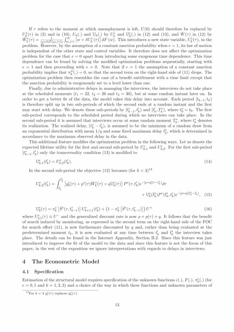
Finally, due to administrative delays in managing the interviews, the interviews do not take placeat the scheduled moments (t1 = 22, t2 = 26 and t3 = 30), but at some random instant later on. Inorder to get a better fit of the data, the model takes this delay into account. Each period [tk−1, tk)is therefore split up in two sub-periods of which the second ends at a random instant and the firstmay start with delay. We denote these sub-periods by [t∗k−1, t

′k) and [t′k, T

∗k ), where t∗0 = t0. The first

sub-period corresponds to the scheduled period during which no interviews can take place. In thesecond sub-period it is assumed that interviews occur at some random moment T ∗

k , where t∗k denotesits realization. The realized delay, (t∗k − t′k), is assumed to be the minimum of a random draw froman exponential distribution with mean 1/q and some fixed maximum delay t∗k, which is determined inaccordance to the maximum observed delay in the data.

This additional feature modifies the optimization problem in the following ways. Let us denote theexpected lifetime utility for the first and second sub-period by U e

k,1 and U ek,2. For the first sub-period

[t∗k−1, t′k) only the transversality condition (13) is modified to

Uek,1(t

′k) = U e

k,2(t′k). (14)

In the second sub-period the objective (12) becomes (for k < 3)13

U ek,2(t

′k) =

∫ t∗k

t′k

[

yeh(τ) + pe(τ)W e

k (τ) + qUek(τ)

]

P e(τ, t′k)e−[ρ+q](τ−t′

k)dτ

+ Uek(t

∗k)P

e(t∗k, t′k)e

−[ρ+q](t∗k−t′

k), (15)

Uek(τ) = πe

k

[

Se(τ, t∗k−1)]

U ek+1,1(t

∗k) +

(

1 − πek

[

Se(τ, t∗k−1)])

U+ (16)

where U e4,1(τ) ≡ U− and the generalized discount rate is now ρ + p(τ) + q. It follows that the benefit

of search induced by monitoring, as expressed in the second term on the right-hand side of the FOCfor search effort (11), is now furthermore discounted by q and, rather than being evaluated at thepredetermined moment tk, it is now evaluated at any time between t′k and t∗k the interview takesplace. The details can be found in the Internet Appendix, Section B.2. Since this feature was justintroduced to improve the fit of the model to the data and since this feature is not the focus of thispaper, in the rest of the exposition we ignore interpretations with regards to delays in interviews.

4 The Econometric Model

4.1 Specification

Estimation of the structural model requires specification of the unknown functions c(.), F (.), πek(.) (for

e = 0, 1 and k = 1, 2, 3) and a choice of the way in which these functions and unknown parameters of

13For k = 3 yeℓ (τ) replaces ye

h(τ).

13

the model (ρ, ν, δ and q) depend on individual characteristics. As to the latter, the level of benefits(bh, bl) is a first source of heterogeneity. In addition, the cost of search and the separation rate dependon gender and three levels of education (low, medium and high),14 which we denote - including theintercept - by x. Computational limitations did not allow for a more extensive dependence on observedor on unobserved characteristics. However, this does not seem that restrictive in this particular study,since the target group of the monitoring scheme is long-term unemployed. Consequently, through thedynamic selection over the unemployment spell, this group is already relatively homogeneous. This isconfirmed by the internal and external validation analysis reported in Sections 6.2 and 6.3.

The relative value of leisure and the job separation rate are specified respectively as ν = exp{ν}and δ(x) = exp{x′ζδ}. As explained in Section 2, the arrival rate of job offers is equal to the level ofsearch effort measured in effective units. This normalization of search effort affects the interpretationonce we allow for heterogeneous workers. Highly-educated workers for instance exert less effort thanlow-educated workers to attain the same effective search intensity. We account for this by allowingthe marginal cost of effective search to depend on individual characteristics. However, we maintainthe assumption that the monitoring is directly (but imperfectly) related to effective search intensityrather than to the underlying effort. The cost of search is chosen such that c(0) = 0, c′(.) > 0 andc′′(.) > 0:

c [s(τ)|x] = exp{

exp{x′ζc}s(τ)}

− 1. (17)

The net wage offer density f(w) is assumed to be log-normal: w ∼ LN (µ, σ). Observed net wagesare measured with a multiplicative error m: wo = w ·m, and the density function of the measurementerror h(m) is a unit-mean log-normal: m ∼ LN

(

−ω2/2, ω)

. Following Christensen and Kiefer (1994),it can be shown that the density function of observed wages fo(w

o; τ) if unemployment is left at τ isgiven by

fo(wo; τ) =

∫ wo/wer(τ)

0

f(wo/m)

F [wer(τ)]

1

mh(m)dm (18)

The probability of being sanctioned at the kth interview (k ∈ {1, 2, 3}) for someone who did notleave unemployment since notification (e = 0) and someone who returned to unemployment after atemporary job (e = 1) takes the following functional form:

π0k

[

S0(

t∗k, t∗k−1

)]

= exp{

−β0k · S0

(

t∗k, t∗k−1

)}

, with, β0k ≥ 0 (19)

π1k = exp{−β1

k}, with, β1k ≥ 0. (20)

In relation with Proposition 3, notice that Ψk = 0.

4.2 Identification

Individuals are sampled after 13 months of UI entitlement (ts ≡ t0 − 1 = 13). The data containinformation on the observed individual characteristics (x), on the UB level that is paid out to eachindividual and on the duration of the unemployment spell (du). For any observed unemploymentspell of length du the data provide information about the timing of monitoring within this spell:The unemployment duration at the moment of notification (t∗0) and the unemployment duration atthe moment of the kth interview ({t∗k}

3k=1), where t∗k = ∅ if the kth interview did not yet take place.

Furthermore, for each observed kth interview the data provide the outcome ({Ok}3k=1) of the evaluation

of job search effort, where Ok = 0 if the outcome is positive, Ok = 1 the outcome is negative andOk = ∅ if the interview did not yet take place.

Whenever the unemployed individual leaves to the destination other than full-time employmentwe right-censor the unemployment duration at the observed length du. Once the destination state is

14Respectively, (i) primary or lower secondary, (ii) upper-secondary education and (iii) higher education.

14

full-time employment, we record the net wage earned at the start of the employment spell (wo) andthe duration of the employment spell (dj). Similar to the duration of unemployment, the observedemployment spell is right-censored if one leaves for destinations other than unemployment.

The values for job search effort se(τ) and the reservation wage wer(τ) at time τ are obtained from

the solution of the optimal control problem as described in Appendix C. These control variables areconditional on functions of x and of all the parameters of the model. To avoid cumbersome expressionswe ignore this dependence in the notation.

Identification of most parameters is quite standard (Flinn and Heckman, 1982; Eckstein andvan den Berg, 2007; Keane et al., 2011). We briefly discuss identification for individuals with agiven set of observed characteristics x and a particular level of UB. Since the log-normal is recoverablefrom a truncated distribution, the observed wages and the parametric assumption on the measurementerror of wages is sufficient to identify the reservation wage, the complete wage offer distribution (µ andσ) and the variance of the measurement error (ω2). Given that the reservation wage and the wage offerdistribution are identified, one can recover the job arrival rate (and hence search intensity)15 from dataon the duration at which jobs are found. In a stationary setting, since the level of UB and the lengthof the scheduled and delay intervals are observed, the relative value of leisure (ν) and the marginalcost of search (and therefore ζc) can be identified from the FOC of the reservation wage and the searcheffort for any given job separation rate (δ), discount rate (ρ) and probability of negative evaluation(πe

k(.), for e ∈ {0, 1} and k ∈ {1, 2, 3}). The parameters of job separation rate ζδ are identified fromthe observed employment durations dj . Since behavior is non-stationary, the discount rate ρ can beidentified from the differential equations describing the time paths of the control variables.16 The pa-rameter βe

1 (for e ∈ {0, 1}) that determines the probability of negative evaluation at the first interviewis identified from the observed outcome (O1) at the first evaluation of job search effort (e = 0) andfrom the observation of an employment experience since notification (e = 1). Since the second andthird evaluation interviews are observed for very few individuals (see Table 4 in Section 5.2), βe

2 andβe

3 are identified from aggregate observations on the outcomes of these evaluations. How this is doneis explained in the next paragraph. Finally, q is identified from observed lengths of interview delays.

Identification of βe2 and βe

3 from aggregate observations of the probability of negative evaluationis achieved under the assumption that βe

k = κkβe1, where κk is a fixed constant independent of e,

and that the sample average of the probability of a negative evaluation at the kth interview (πk) isproportional to the aggregate observed probability of negative evaluation (πa

k) presented in Table 1,i.e. ∀k ∈ {1, 2, 3} : πk = f · πa

k , where f is a fixed constant independent of k. With these assumptionsκk (and therefore βk) for k = 2 and k = 3 can be found by solving the following implicit equation:πk(κk) = f ·πa

k = π1πa1πa

k , where it is made explicit that πk is a function of κk and where all terms on the

right-hand side are known or can be estimated (π1). A complication is that the aggregate probabilityof negative evaluation is conditional on being evaluated at the kth interview, while the sample averageis calculated for the sample of notified individuals for whom these evaluations are not all observed.The sample average probability of negative evaluation is therefore estimated by a weighted sum ofexpected individual probabilities of negative evaluation (all of which a function of κk). The weightsreflect that the likelihood of evaluation is not equal across notified individuals. In Appendix B it isshown how this weighted sum is constructed.

4.3 Likelihood Contributions

To write down the likelihood contribution of an unemployed individual consider first the probabilityof surviving in unemployment until some given moment t. For that, let p0(τ) be given by (4) with su-perscript e = 0 denoting that the worker did not leave unemployment since t0, and let p+ ≡ s+F (w+

r ).

15Since we have no information on the intensity of search effort, we identify search effort with the job arrival rate (seeSection 2).

16These differential equations provide over-identifying restrictions for the other parameters.

15

Furthermore define t′k ≡ min{t, t′k}, t∗k ≡ min{t, t∗k} and t′4 ≡ t∗4 ≡ ∞. With these definitions, theprobability of surviving in unemployment until t, being notified at t∗0 and being evaluated at {t∗k}

3k=1,

conditional on being unemployed at sample selection, i.e. at ts ≡ t∗0 − 1, and on the outcome of thenotification (O0 ≡ 1) and of the evaluations ({Ok}

3k=1) is

P(

t, {t∗k}3k=0 |ts, {Ok}

3k=0

)

= exp{

−(t∗0 − ts)p+}

× exp

{

−1[t ≥ t∗0]4

∑

k=1

Ok−1

[

∫ t′k

t∗k−1

p0(τ)dτ + 1[t ≥ t′k]

∫ t∗k

t′k

[p0(τ) + q]dτ

] }

×3

∏

k=1

q1[t≥t∗k] exp

{

−3

∑

k=1

(1 − Ok)(t − t∗k)p+

}

. (21)

Note that if O3 = 1,∀τ > t∗3, e ∈ {0, 1} : pe(τ) = p− ≡ s−F (w−r ). The first term on the right-hand

side in (21) is the survivor rate in unemployment between sample selection ts and t or the notificationt∗0, depending on which of the two comes first. The term following on the next line gives for each k thesurvivor rates in the scheduled interval [t∗k−1, t

′k) and in the delay interval [t′k, t

∗k). In the latter interval

re-employment and the occurrence of an evaluation are competing risks, which explains the presenceof q in the expression. However, if an evaluation takes place, the worker still remains unemployed.Consequently, the probability of surviving in unemployment after t∗k is the density of being evaluatedat t∗k times the probability of surviving in unemployment beyond t∗k. Since this density at t∗k is theproduct of the arrival rate of evaluation q and the corresponding survivor function, this explains thepresence of q in the last term on the third line on the right-hand side of (21). The last term alsocontains the survivor rate in unemployment after a positive evaluation at any interview k.

The duration data are grouped into monthly intervals. We account for this grouping by integratingover the corresponding time intervals and by assuming that at most one transition occurs within aninterval. With the result in (21), an individual contribution of an unemployment spell lasting du

months, conditional on the outcomes of the evaluations, writes

ℓ (du, dj , wo) =

∫ du

du−1p0(τ)P

(

τ, {t∗k}3k=0 |ts, {Ok}

3k=0

)

[fo(wo; τ)]cw dτ

× [exp {−δ(dj − 1)} − ce exp {−δde}] (22)

where ce = 0 if the employment spell that follows the transition from unemployment is right censored(ce = 1 otherwise), and cw = 0 if the wage upon this transition is unobserved (cw = 1 otherwise).Whenever the unemployment spell is right-censored, neither dj nor wo are observed any longer. Inthis case the contribution to the likelihood (22) reduces to the survivor probability (21) evaluated att = du.

Finally, the likelihood function for the realized evaluation outcomes at the first interview is

ℓ (O1, e) =[

exp{

−β01 S0(t∗1, t

∗0)

}O1(

1 − exp{

−β01 S0(t∗1, t

∗0)

})1−O1]1−e

×[

exp{

−β11

}O1(

1 − exp{

−β11

})1−O1]e

(23)

for e ∈ {0, 1}. Appendix C describes in detail how the model is solved and estimated.

5 Data

5.1 Sample Selection Criteria

The data originate from several administrative sources: (i) the federal UI agency for monthly infor-mation on UB claims and the new monitoring procedure; (ii) various Social Security institutions for

16

information about employment spells (including self-employment) and earnings (for salaried workers).Our model does not explain the choice of working hours. Hence, as in the theoretical part, we restrictattention to jobs registered as full-time occupations. This information is available from January 2001until the end of 2006.

As of July 2004, the notification in the new monitoring procedure was sent only to individuals whowere younger than 30 years old. Our sample ignores individuals who were at that moment youngerthan 25 years old. The standardized average unemployment rate lies in the range between 4 and 5%among the 25-49 years old during the period 2004-2006 in the region under consideration. Despitethese relatively good performances, about 45% of the total stock of unemployed was jobless for morethan a year.

In order to determine the population to whom notifications are sent in a particular month (e.g.in July), the administration actually selects individuals who have been unemployed 13 months ormore according to the information available at the end of the second month prior to the month ofdispatch of the notification (on May 31 in the example). Our sample contains individuals for whomthe entitlement duration was exactly 13 months at the end of each month between May and August2004 and to whom therefore a notification was sent between July and October, 2004 if they were stillUI claimants at that time. In accordance with the theoretical part of this paper, the notified peopleare entitled to a flat UB for an indefinite duration (except if they are sanctioned of course).17 Thesecriteria lead to a sample of 903 individuals. We also selected a sample according to exactly the samecriteria one year earlier, in 2003. This pre-program data set made of 883 individuals will be used inthe validation exercise in Subsection 6.3.

Note, since sampled individuals may have found a job between the selection date and the receiptof the notification, we can check whether claimants anticipate the notification. Cockx and Dejemeppe(2010) cannot find any evidence of such an anticipation (see their section 6.1.2). This means that wecan safely assume that the moment of notification corresponds to t0 in the theoretical model.

5.2 Descriptive Statistics

Table 2 reports summary statistics respectively for the sample selected in 2004 and 2003. Time-varyingvariables are evaluated at the sampling date. Monthly earnings are measured at the start of a salariedemployment spell. All monetary variables are measured in 2004 euros. Table 2 reports informationwith respect to the observed characteristics that we actually use: gender, the level of education, thehousehold type determining the benefit level (head of household, single or cohabitant) and the typeof entitlement (school-leaver or work experience). The monthly levels of benefits bh vary between325e and 1005e, with an average in 2004 of 646e and a coefficient of variation of 37%. Monthly netearnings amount to 1,200e on average (with a coefficient of variation of 23%). These statistics arenot very different for the sample selected in 2003. Table 3 provides the levels of the benefit, if any, incase of a sanction. Recall that there is no sanction after a first negative evaluation. The magnitudeof the sanction is the same after the second and third negative evaluation. However, the sanction istemporary after the second while the entitlement to UB is completely lost after the third evaluation.The magnitude of the loss bh − bl lies in the range [0, 385] e/month (the lowest and the highest valueof the sanction is presented for category in Table 3).18

Table 4 displays the number of claimants at the various steps of procedure and the outcomes ofeach evaluation in the 2004 sample. Since individuals in this sample may have found a job betweenthe selection date and the notification, only 723 of the 903 sampled individuals are notified. Amongthose notified, 162 attend the first interview. Due to the length of the evaluation procedure, as wellas delays in the scheduled timing and frequent exits out of unemployment before the interviews takes

17For cohabitants, this is not always the case. For them, we only retain those entitled to a flat benefit.18The absence of sanction for some school leavers is due to the equivalence between unemployment insurance benefits

and assistance benefits for this category. This concerns about 7% of the sample.

17

Table 2: Descriptive Statistics by Sample

2004 2003

Number of individuals 903 883

Gender

Women 45.2% 46.2%

Schooling levela

Primary or lower secondary 34.8% 36.8%Upper-secondary 40.0% 42.4%Higher education 25.2% 20.8%

Type of entitlementa (monthly UB level in 2004 e)

Entitled by work experience 69.2% 72.7%Head of household ([865e-1005e]) 22.1% 24.8%Single ([725e-835e]) 32.7% 33.7%Cohabitant (385e) 14.4% 14.2%

Entitled by schooling 30.8% 27.3%

Head of household (835e) 1.8% 2.3%Single (595e) 7.2% 6.8%Cohabitant (325e) 21.8% 18.2%

Unemployment benefitsa

Mean (2004 e) 646 666Standard deviation (242) (235)25% 385 385Median 725 75575% 835 845

Observed net monthly earnings (1st spell)

Number of individuals 427 358Mean (2004 e) 1,199 1,228Standard deviation (279) (265)25% 1,066 1,100Median 1,214 1,25075% 1,358 1,381

aAt the sample selection date.

18

Table 3: Benefit Levels in Case of a Sanction and Size of Sanction (Monthly Level in 2004e)

2nd and 3rd interview Min. sanction Max. sanction

Type of entitlementa

Entitled by work experience

Head of household ([865e-1005e]) 802 e 63e 203eSingle ([725e-835e]) 601 e 124e 234eCohabitant (385e) 0 385e 385e

Entitled by schooling

Head of household (835e) 802 e 33e 33eSingle (595e) 595 e 0 0Cohabitant (325e) 0 325e 325e

aAt the sample selection date.

place, only very few sampled individuals are evaluated for a second and third time. Subsection 4.2has explained how we deal with the low observed number of participants in these evaluations.

Table 4: Sampled Population at Each Step of the Monitoring Procedurea

Number of individuals 903

Steps of the monitoring procedure

Notification letter 723(80.1%)

First interview 162(17.9%)

Positive evaluation 112(69.1%)

Negative evaluation 50(30.9%)

Second interview 18(36.0%)

Positive evaluation 16Negative evaluation 2Third interview 1

(50.0%)Positive evaluation 1Negative evaluation 0

a% in the population at risk.

19

6 Results

6.1 Estimated Parameters

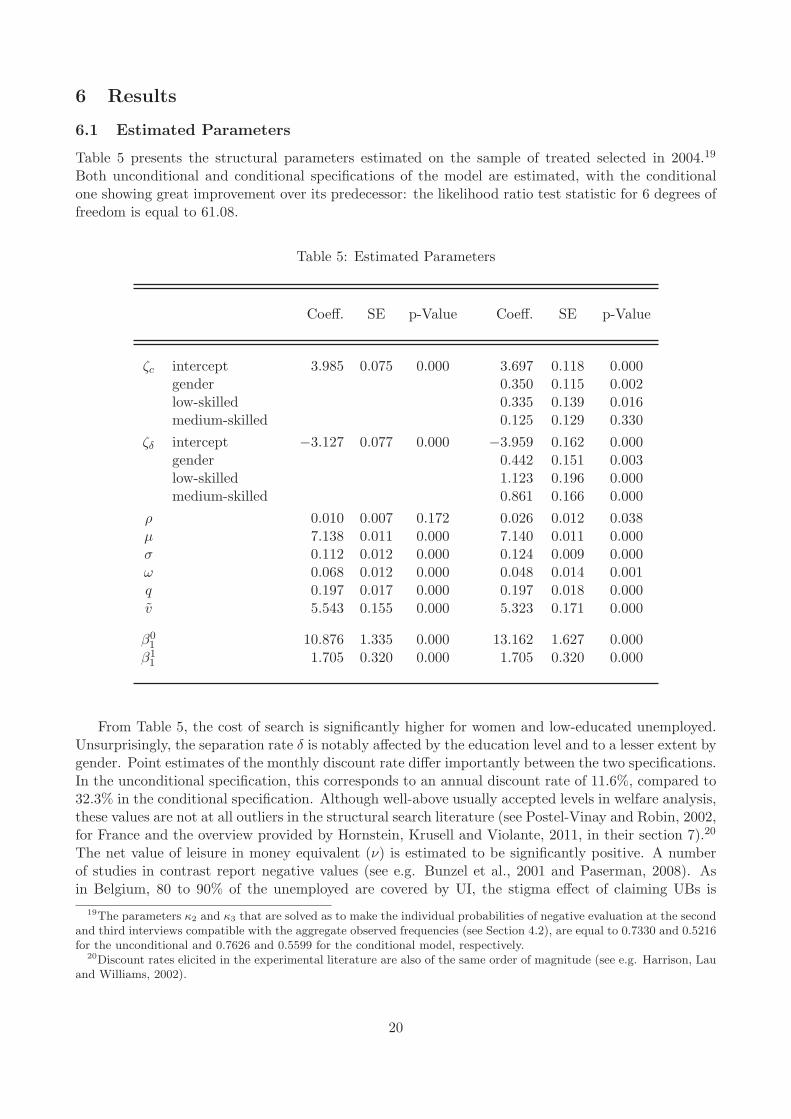
Table 5 presents the structural parameters estimated on the sample of treated selected in 2004.19

Both unconditional and conditional specifications of the model are estimated, with the conditionalone showing great improvement over its predecessor: the likelihood ratio test statistic for 6 degrees offreedom is equal to 61.08.

Table 5: Estimated Parameters

Coeff. SE p-Value Coeff. SE p-Value

ζc intercept 3.985 0.075 0.000 3.697 0.118 0.000gender 0.350 0.115 0.002low-skilled 0.335 0.139 0.016medium-skilled 0.125 0.129 0.330

ζδ intercept −3.127 0.077 0.000 −3.959 0.162 0.000gender 0.442 0.151 0.003low-skilled 1.123 0.196 0.000medium-skilled 0.861 0.166 0.000

ρ 0.010 0.007 0.172 0.026 0.012 0.038µ 7.138 0.011 0.000 7.140 0.011 0.000σ 0.112 0.012 0.000 0.124 0.009 0.000ω 0.068 0.012 0.000 0.048 0.014 0.001q 0.197 0.017 0.000 0.197 0.018 0.000v 5.543 0.155 0.000 5.323 0.171 0.000

β01 10.876 1.335 0.000 13.162 1.627 0.000

β11 1.705 0.320 0.000 1.705 0.320 0.000

From Table 5, the cost of search is significantly higher for women and low-educated unemployed.Unsurprisingly, the separation rate δ is notably affected by the education level and to a lesser extent bygender. Point estimates of the monthly discount rate differ importantly between the two specifications.In the unconditional specification, this corresponds to an annual discount rate of 11.6%, compared to32.3% in the conditional specification. Although well-above usually accepted levels in welfare analysis,these values are not at all outliers in the structural search literature (see Postel-Vinay and Robin, 2002,for France and the overview provided by Hornstein, Krusell and Violante, 2011, in their section 7).20

The net value of leisure in money equivalent (ν) is estimated to be significantly positive. A numberof studies in contrast report negative values (see e.g. Bunzel et al., 2001 and Paserman, 2008). Asin Belgium, 80 to 90% of the unemployed are covered by UI, the stigma effect of claiming UBs is

19The parameters κ2 and κ3 that are solved as to make the individual probabilities of negative evaluation at the secondand third interviews compatible with the aggregate observed frequencies (see Section 4.2), are equal to 0.7330 and 0.5216for the unconditional and 0.7626 and 0.5599 for the conditional model, respectively.

20Discount rates elicited in the experimental literature are also of the same order of magnitude (see e.g. Harrison, Lauand Williams, 2002).

20

presumably lower than elsewhere. Finally, the standard error of the measurement error of wages issmall (about 5%). This is a first evidence of the goodness-of-fit of the model, to which we turn now.

6.2 Internal Validation: Goodness-of-fit

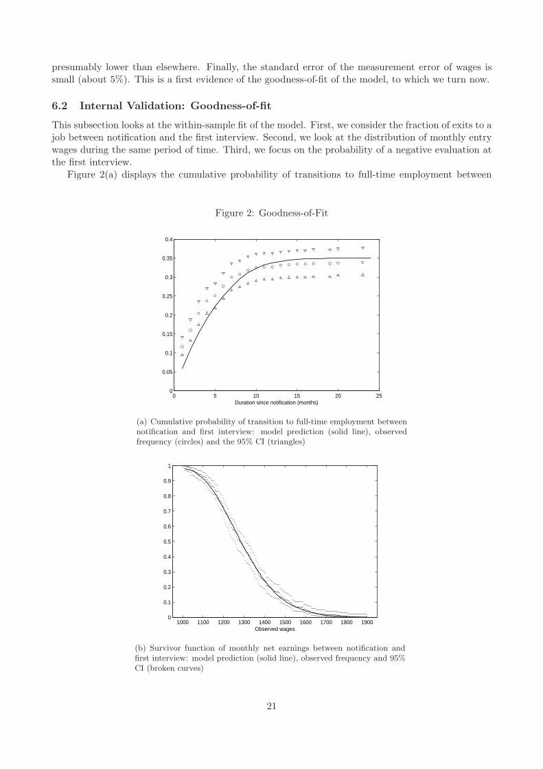
This subsection looks at the within-sample fit of the model. First, we consider the fraction of exits to ajob between notification and the first interview. Second, we look at the distribution of monthly entrywages during the same period of time. Third, we focus on the probability of a negative evaluation atthe first interview.

Figure 2(a) displays the cumulative probability of transitions to full-time employment between

Figure 2: Goodness-of-Fit

0 5 10 15 20 250

0.05

0.1

0.15

0.2

0.25

0.3

0.35

0.4

Duration since notification (months)

(a) Cumulative probability of transition to full-time employment betweennotification and first interview: model prediction (solid line), observedfrequency (circles) and the 95% CI (triangles)

1000 1100 1200 1300 1400 1500 1600 1700 1800 19000

0.1

0.2

0.3

0.4

0.5

0.6

0.7

0.8

0.9

1

Observed wages

(b) Survivor function of monthly net earnings between notification andfirst interview: model prediction (solid line), observed frequency and 95%CI (broken curves)

21

notification and the first interview. The horizontal axis measures actual duration since notification.Using the point estimates of the structural model, the theoretical distribution of exits to employmentcan be computed for each notified member of the sample. The solid line is the average of thesedistributions. This curve reaches a horizontal asymptote at about 0.35 because as time goes bymore and more unemployed become interviewed for the first time or exit to nonemployment. Toplot the circles, we have used the nonparametric estimate of the cumulative probability of transitionsto full-time employment in the absence of regressors. Confidence intervals (CI) were computed bynonparametric bootstrap. We have drawn 5000 times from the original sample with replacement.The upper and lower triangles in Figure 2(a) correspond to the 0.025 and the 0.975 percentiles of theaforementioned cumulative probability. The fit is reasonable overall, and with the 95% CI startingfrom the fourth month since notification.

Figure 2(b) displays the survivor function of monthly net accepted earnings. To compute it, oneneeds the reservation wage. Based on the point estimates, three theoretical duration distributionscan be computed for each individual, with respectively full-time employment, the first interview andthe residual state as destinations. Taking 50 random draws from these distributions for each notifiedindividual, an exit to employment obtains when the duration to this destination is the shortest one.Then, the reservation wage is calculated for the duration at which the unemployed exits to a job.With this information, the theoretical distribution of accepted earnings (with measurement errors) iscomputed. Finally, the average taken over all notified individuals leads to the solid and thick curve inFigure 2(b). The thin broken curve which is close to the latter is the Kaplan-Meier survivor functioncalculated on the basis of observed accepted earnings. The upper and lower broken curves providethe corresponding 95% CI. The fit of wage distribution turns out to be perfect throughout its entiresupport.

The correct specification of the probability of negative evaluation (at the first interview) is checkedby testing the equality of theoretical frequencies of negative evaluation at the first interview to theobserved frequencies. The Pearson chi-square goodness-of-fit test is asymptotically ∼ χ2

(1) and thep-value is 0.31, confirming the absence of significant difference between the data and the model pre-diction.

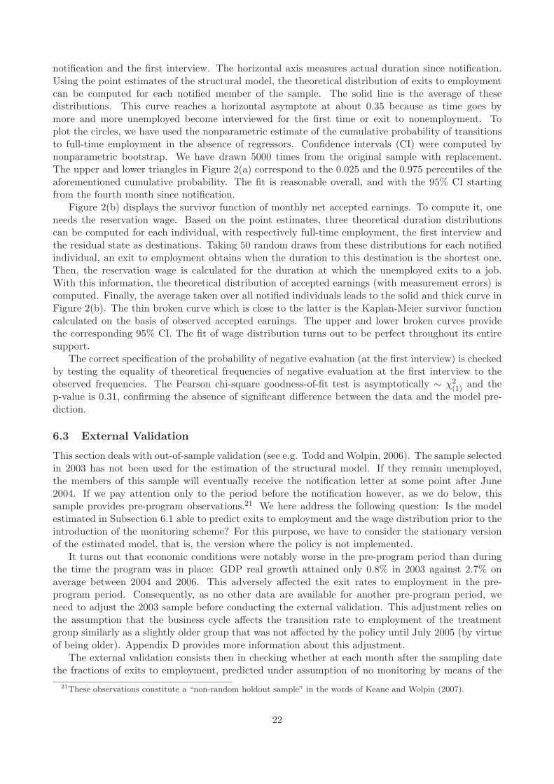
6.3 External Validation

This section deals with out-of-sample validation (see e.g. Todd and Wolpin, 2006). The sample selectedin 2003 has not been used for the estimation of the structural model. If they remain unemployed,the members of this sample will eventually receive the notification letter at some point after June2004. If we pay attention only to the period before the notification however, as we do below, thissample provides pre-program observations.21 We here address the following question: Is the modelestimated in Subsection 6.1 able to predict exits to employment and the wage distribution prior to theintroduction of the monitoring scheme? For this purpose, we have to consider the stationary versionof the estimated model, that is, the version where the policy is not implemented.

It turns out that economic conditions were notably worse in the pre-program period than duringthe time the program was in place: GDP real growth attained only 0.8% in 2003 against 2.7% onaverage between 2004 and 2006. This adversely affected the exit rates to employment in the pre-program period. Consequently, as no other data are available for another pre-program period, weneed to adjust the 2003 sample before conducting the external validation. This adjustment relies onthe assumption that the business cycle affects the transition rate to employment of the treatmentgroup similarly as a slightly older group that was not affected by the policy until July 2005 (by virtueof being older). Appendix D provides more information about this adjustment.

The external validation consists then in checking whether at each month after the sampling datethe fractions of exits to employment, predicted under assumption of no monitoring by means of the

21These observations constitute a “non-random holdout sample” in the words of Keane and Wolpin (2007).

22

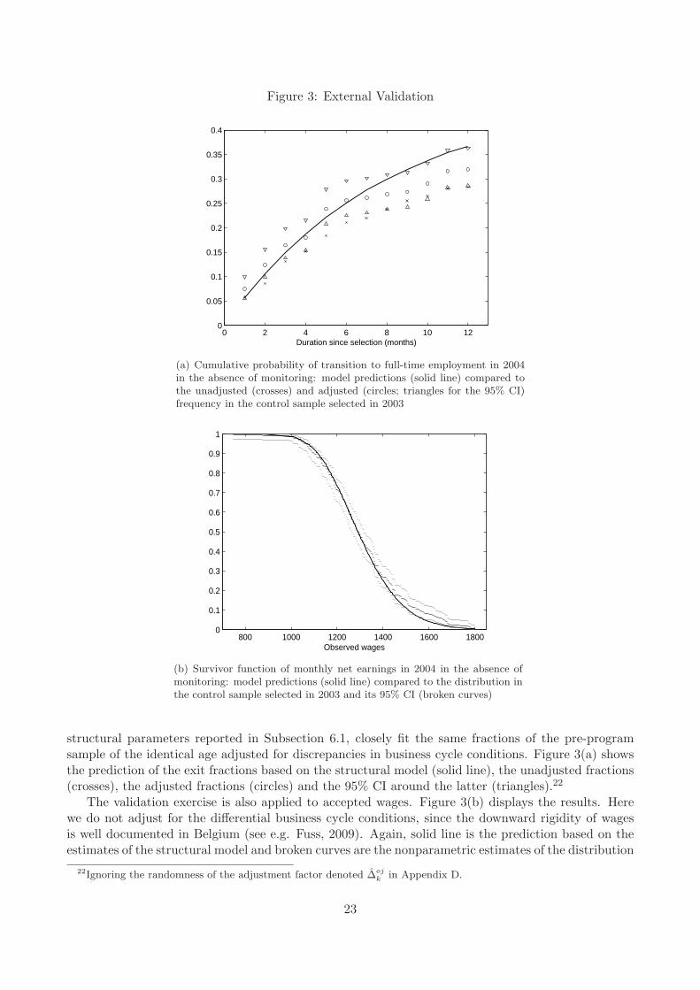
Figure 3: External Validation

0 2 4 6 8 10 120

0.05

0.1

0.15

0.2

0.25

0.3

0.35

0.4

Duration since selection (months)

(a) Cumulative probability of transition to full-time employment in 2004in the absence of monitoring: model predictions (solid line) compared tothe unadjusted (crosses) and adjusted (circles; triangles for the 95% CI)frequency in the control sample selected in 2003

800 1000 1200 1400 1600 18000

0.1

0.2

0.3

0.4

0.5

0.6

0.7

0.8

0.9

1

Observed wages

(b) Survivor function of monthly net earnings in 2004 in the absence ofmonitoring: model predictions (solid line) compared to the distribution inthe control sample selected in 2003 and its 95% CI (broken curves)

structural parameters reported in Subsection 6.1, closely fit the same fractions of the pre-programsample of the identical age adjusted for discrepancies in business cycle conditions. Figure 3(a) showsthe prediction of the exit fractions based on the structural model (solid line), the unadjusted fractions(crosses), the adjusted fractions (circles) and the 95% CI around the latter (triangles).22

The validation exercise is also applied to accepted wages. Figure 3(b) displays the results. Herewe do not adjust for the differential business cycle conditions, since the downward rigidity of wagesis well documented in Belgium (see e.g. Fuss, 2009). Again, solid line is the prediction based on theestimates of the structural model and broken curves are the nonparametric estimates of the distribution

22Ignoring the randomness of the adjustment factor denoted ∆ojk in Appendix D.

23

of observed wages, along with the corresponding CI.Figures 3(a-b) firmly establish an excellent out of sample fit of the model in the environment with

no policy. This validates that we can use the parameter estimates of the structural model to constructthe counterfactual no-treatment outcomes for the treated sample and underscores the reliability of theAverage Treatment Effects on the Treated (ATT) reported in Subsection 7.1.

6.4 Interpretation of Estimation Results Based on Simulations

Before reporting the average treatment effects, we simulate the estimated model for the treated sample.The aim is to gain insight into the behavioral adjustment of the unemployed as predicted by the model.The model is simulated for each unemployed in the sample under the assumption that each evaluationturns out to be negative. This choice is made here on purpose to keep the composition of the sampleunchanged all along the the different stages of the monitoring scheme. Figure 4 displays the sampleaverage of these paths. It comprises four panels. The upper-right panel displays average effective searcheffort levels. The measurement unit on the vertical axis is the monthly probability of a job-offer. Thelower panels display the monthly net reservation wage (in euros) and the acceptance rate. Finally theupper-left panel provides the monthly exit rate towards full-time employment. On the horizontal axis,duration, measured in months, is normalized to zero at notification. Solid lines represent the caseof an unemployed without an employment spell in the relevant period (e = 0) while the interruptedlines correspond to someone with such an employment spell (e = 1). Before notification, the averagemonthly exit rate equals 0.061 (implying an expected unemployment duration of 16.4 months in astationary environment) and the acceptance rate is on average somewhat above 85%.23

Let us first consider the case e = 1. If the unemployed is recruited after notification (k = 0)or after a negative evaluation (k ∈ {1, 2}) and if she returns to unemployment, the probability of anegative evaluation π1

k+1 is given by (20) and hence the expected utility before any interview (13) is notaffected by accumulated search effort S1(tk+1, tk). The interrupted line describes the average path foran individual who finds a job after each stage of the scheme and returns to unemployment immediatelyafter. Between notification and the first interview (where π1

1 = 0.18), search effort and the reservationwage varies only slightly. The fact that a first negative evaluation only results in signing an action planwithout any monetary sanction explains this. After the first negative assessment of search effort, thedecision variables adjust somewhat more than previously, since the individual approaches the secondevaluation at which she risks a temporary monetary sanction of the size indicated in Table 3. Theeffect of this sanction is especially apparent in the discontinuous jumps of the decision variables rightafter the second negative evaluation. Between the second and the third interview, however, searcheffort declines and the reservation increases. To understand this, remember that the level of benefitsis not further reduced if the unemployed is negatively evaluated at the third interview. Conversely, ifthis evaluation is positive, the unemployed regains her entitlement to the high benefit level. So, theexpected utility after the third evaluation is higher than the current expected utility between the secondnegative evaluation and the third interview. Consequently, as time evolves, the prospect of benefitingfrom this improvement gets closer and is increasingly valued because of discounting. The permanentloss of UB entitlement when the third evaluation is negative abruptly enhances further search effortand pushes the reservation wage further down. As of that moment, the average acceptance rate equals95%.24

Figure 4 also shows that the average paths are substantially different if no job is found throughoutthe monitoring process (e = 0) and the probability of negative evaluation π0

k

[

S0(

t∗k, t∗k−1

)]

for k ∈{1, 2, 3} is effort dependent, as in (19). The level of search effort (resp. reservation wage) is everywhere

23Note that these values also apply after a positive evaluation at any of the three interviews.24Comparing the exit rate after the third negative evaluation to the one before notification provides the ex-post

effect induced by an unanticipated withdrawal of UB. This would increase the exit rate to full-time employment by 1.3percentage points on average (namely, 0.074 − 0.061), which amounts to a relative increase of 21%.

24

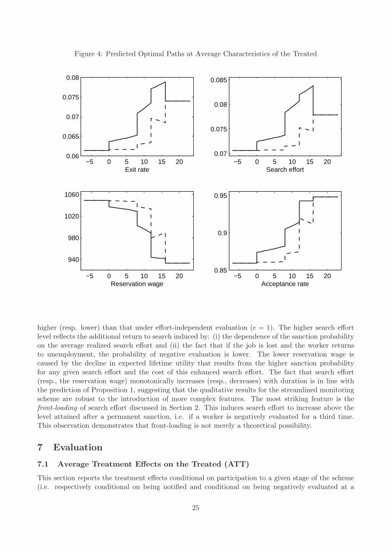
Figure 4: Predicted Optimal Paths at Average Characteristics of the Treated

−5 0 5 10 15 200.06

0.065

0.07

0.075

0.08

Exit rate−5 0 5 10 15 20

0.07

0.075

0.08

0.085

Search effort

−5 0 5 10 15 20

940

980

1020

1060

Reservation wage−5 0 5 10 15 20

0.85

0.9

0.95

Acceptance rate

higher (resp. lower) than that under effort-independent evaluation (e = 1). The higher search effortlevel reflects the additional return to search induced by: (i) the dependence of the sanction probabilityon the average realized search effort and (ii) the fact that if the job is lost and the worker returnsto unemployment, the probability of negative evaluation is lower. The lower reservation wage iscaused by the decline in expected lifetime utility that results from the higher sanction probabilityfor any given search effort and the cost of this enhanced search effort. The fact that search effort(resp., the reservation wage) monotonically increases (resp., decreases) with duration is in line withthe prediction of Proposition 1, suggesting that the qualitative results for the streamlined monitoringscheme are robust to the introduction of more complex features. The most striking feature is thefront-loading of search effort discussed in Section 2. This induces search effort to increase above thelevel attained after a permanent sanction, i.e. if a worker is negatively evaluated for a third time.This observation demonstrates that front-loading is not merely a theoretical possibility.

7 Evaluation

7.1 Average Treatment Effects on the Treated (ATT)

This section reports the treatment effects conditional on participation to a given stage of the scheme(i.e. respectively conditional on being notified and conditional on being negatively evaluated at a

25

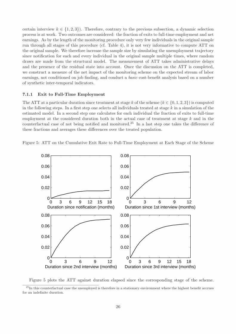
certain interview k ∈ {1, 2, 3}). Therefore, contrary to the previous subsection, a dynamic selectionprocess is at work. Two outcomes are considered: the fraction of exits to full-time employment and netearnings. As by the length of the monitoring procedure only very few individuals in the original samplerun through all stages of this procedure (cf. Table 4), it is not very informative to compute ATT onthe original sample. We therefore increase the sample size by simulating the unemployment trajectorysince notification for each and every individual in the original sample multiple times, where randomdraws are made from the structural model. The measurement of ATT takes administrative delaysand the presence of the residual state into account. Once the discussion on the ATT is completed,we construct a measure of the net impact of the monitoring scheme on the expected stream of laborearnings, not conditioned on job finding, and conduct a basic cost-benefit analysis based on a numberof synthetic inter-temporal indicators.

7.1.1 Exit to Full-Time Employment

The ATT at a particular duration since treatment at stage k of the scheme (k ∈ {0, 1, 2, 3}) is computedin the following steps. In a first step one selects all individuals treated at stage k in a simulation of theestimated model. In a second step one calculates for each individual the fraction of exits to full-timeemployment at the considered duration both in the actual case of treatment at stage k and in thecounterfactual case of not being notified and monitored.25 In a last step one takes the difference ofthese fractions and averages these differences over the treated population.

Figure 5: ATT on the Cumulative Exit Rate to Full-Time Employment at Each Stage of the Scheme

0 3 6 9 12 15 180

0.02

0.04

0.06

0.08

Duration since notification (months)0 3 6 9 12

0

0.02

0.04

0.06

0.08

Duration since 1st interview (months)

0 3 6 9 120

0.02

0.04

0.06

0.08

Duration since 2nd interview (months)0 3 6 9 12 15 18

0

0.02

0.04

0.06

0.08

Duration since 3rd interview (months)

Figure 5 plots the ATT against duration elapsed since the corresponding stage of the scheme.

25In this counterfactual case the unemployed is therefore in a stationary environment where the highest benefit accruesfor an indefinite duration.

26

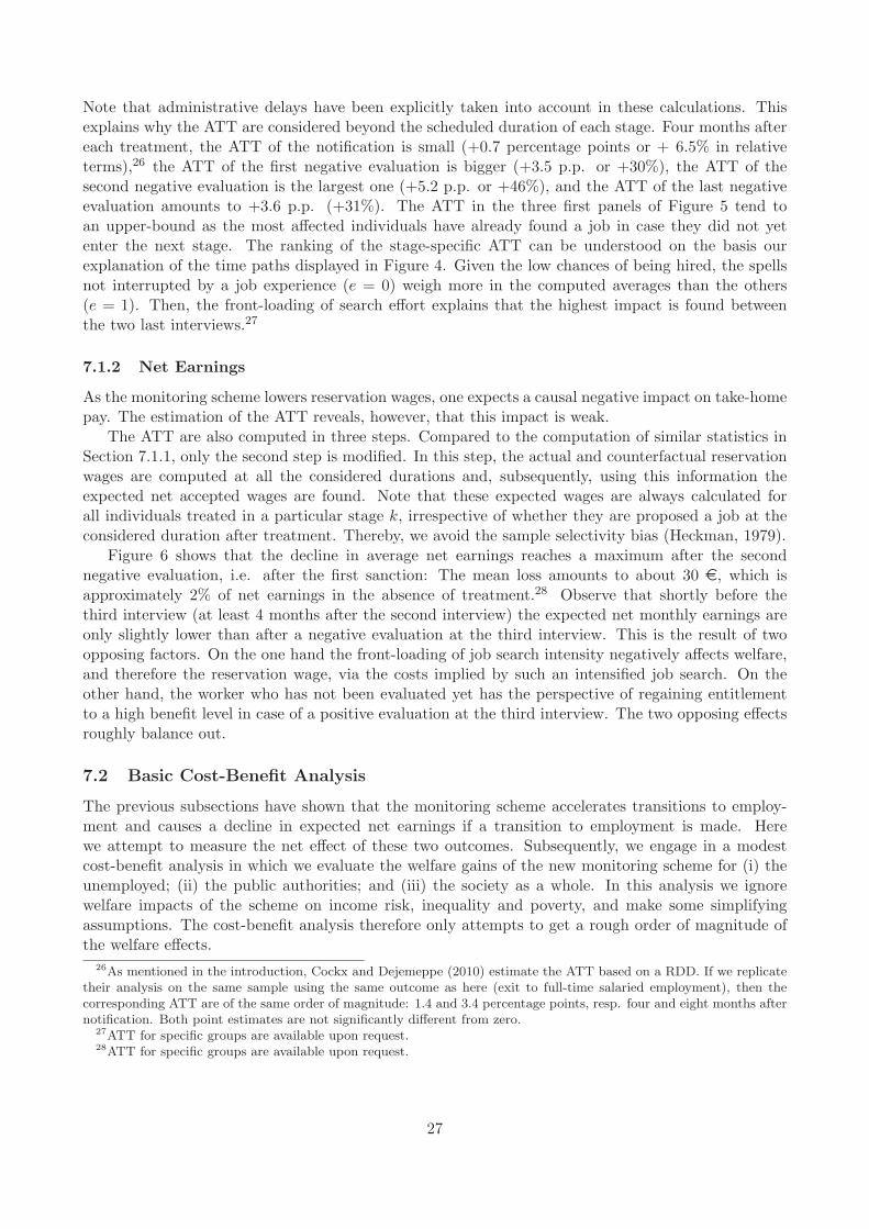
Note that administrative delays have been explicitly taken into account in these calculations. Thisexplains why the ATT are considered beyond the scheduled duration of each stage. Four months aftereach treatment, the ATT of the notification is small (+0.7 percentage points or + 6.5% in relativeterms),26 the ATT of the first negative evaluation is bigger (+3.5 p.p. or +30%), the ATT of thesecond negative evaluation is the largest one (+5.2 p.p. or +46%), and the ATT of the last negativeevaluation amounts to +3.6 p.p. (+31%). The ATT in the three first panels of Figure 5 tend toan upper-bound as the most affected individuals have already found a job in case they did not yetenter the next stage. The ranking of the stage-specific ATT can be understood on the basis ourexplanation of the time paths displayed in Figure 4. Given the low chances of being hired, the spellsnot interrupted by a job experience (e = 0) weigh more in the computed averages than the others(e = 1). Then, the front-loading of search effort explains that the highest impact is found betweenthe two last interviews.27

7.1.2 Net Earnings

As the monitoring scheme lowers reservation wages, one expects a causal negative impact on take-homepay. The estimation of the ATT reveals, however, that this impact is weak.

The ATT are also computed in three steps. Compared to the computation of similar statistics inSection 7.1.1, only the second step is modified. In this step, the actual and counterfactual reservationwages are computed at all the considered durations and, subsequently, using this information theexpected net accepted wages are found. Note that these expected wages are always calculated forall individuals treated in a particular stage k, irrespective of whether they are proposed a job at theconsidered duration after treatment. Thereby, we avoid the sample selectivity bias (Heckman, 1979).

Figure 6 shows that the decline in average net earnings reaches a maximum after the secondnegative evaluation, i.e. after the first sanction: The mean loss amounts to about 30 e, which isapproximately 2% of net earnings in the absence of treatment.28 Observe that shortly before thethird interview (at least 4 months after the second interview) the expected net monthly earnings areonly slightly lower than after a negative evaluation at the third interview. This is the result of twoopposing factors. On the one hand the front-loading of job search intensity negatively affects welfare,and therefore the reservation wage, via the costs implied by such an intensified job search. On theother hand, the worker who has not been evaluated yet has the perspective of regaining entitlementto a high benefit level in case of a positive evaluation at the third interview. The two opposing effectsroughly balance out.

7.2 Basic Cost-Benefit Analysis

The previous subsections have shown that the monitoring scheme accelerates transitions to employ-ment and causes a decline in expected net earnings if a transition to employment is made. Herewe attempt to measure the net effect of these two outcomes. Subsequently, we engage in a modestcost-benefit analysis in which we evaluate the welfare gains of the new monitoring scheme for (i) theunemployed; (ii) the public authorities; and (iii) the society as a whole. In this analysis we ignorewelfare impacts of the scheme on income risk, inequality and poverty, and make some simplifyingassumptions. The cost-benefit analysis therefore only attempts to get a rough order of magnitude ofthe welfare effects.

26As mentioned in the introduction, Cockx and Dejemeppe (2010) estimate the ATT based on a RDD. If we replicatetheir analysis on the same sample using the same outcome as here (exit to full-time salaried employment), then thecorresponding ATT are of the same order of magnitude: 1.4 and 3.4 percentage points, resp. four and eight months afternotification. Both point estimates are not significantly different from zero.

27ATT for specific groups are available upon request.28ATT for specific groups are available upon request.

27

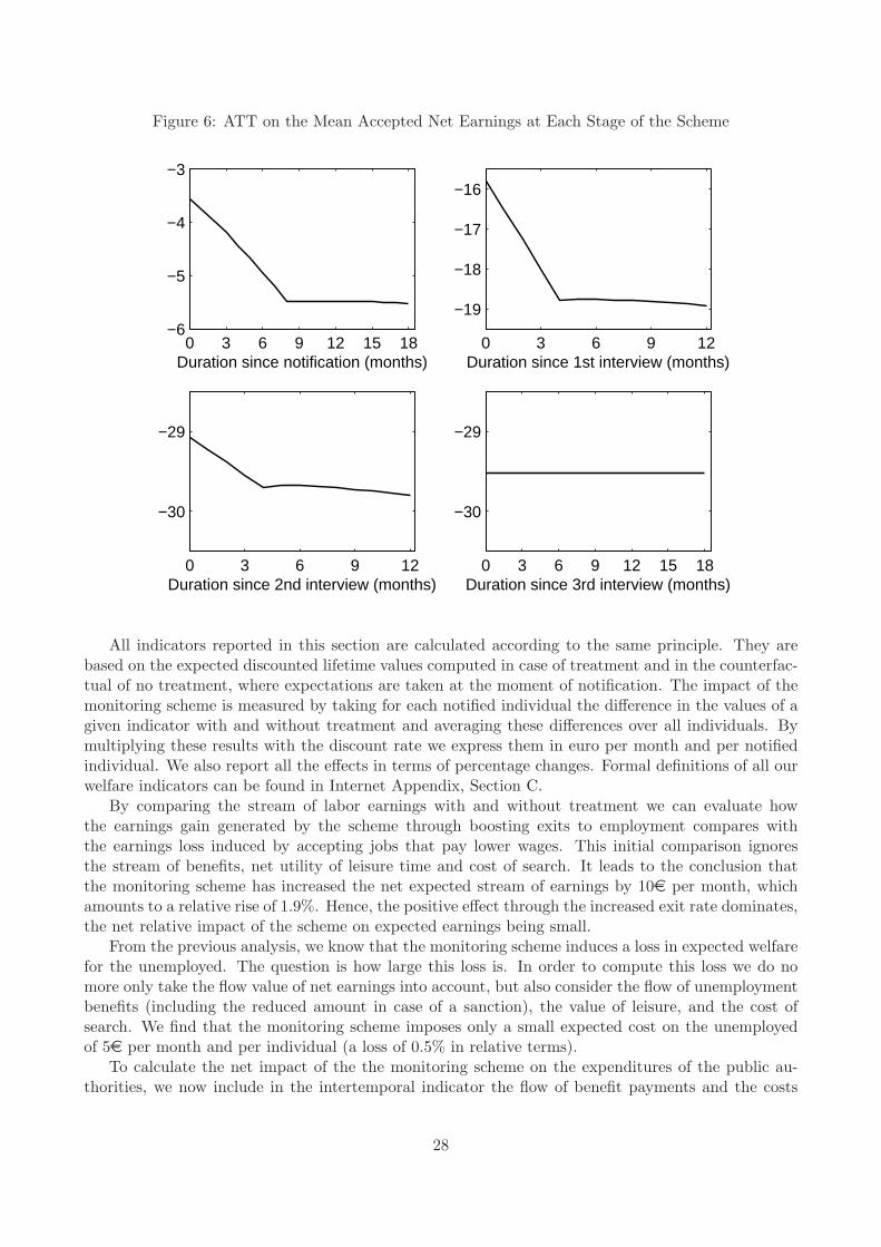
Figure 6: ATT on the Mean Accepted Net Earnings at Each Stage of the Scheme

0 3 6 9 12 15 18−6

−5

−4

−3

Duration since notification (months)0 3 6 9 12

−19

−18

−17

−16

Duration since 1st interview (months)

0 3 6 9 12

−30

−29

Duration since 2nd interview (months)0 3 6 9 12 15 18

−30

−29

Duration since 3rd interview (months)

All indicators reported in this section are calculated according to the same principle. They arebased on the expected discounted lifetime values computed in case of treatment and in the counterfac-tual of no treatment, where expectations are taken at the moment of notification. The impact of themonitoring scheme is measured by taking for each notified individual the difference in the values of agiven indicator with and without treatment and averaging these differences over all individuals. Bymultiplying these results with the discount rate we express them in euro per month and per notifiedindividual. We also report all the effects in terms of percentage changes. Formal definitions of all ourwelfare indicators can be found in Internet Appendix, Section C.

By comparing the stream of labor earnings with and without treatment we can evaluate howthe earnings gain generated by the scheme through boosting exits to employment compares withthe earnings loss induced by accepting jobs that pay lower wages. This initial comparison ignoresthe stream of benefits, net utility of leisure time and cost of search. It leads to the conclusion thatthe monitoring scheme has increased the net expected stream of earnings by 10e per month, whichamounts to a relative rise of 1.9%. Hence, the positive effect through the increased exit rate dominates,the net relative impact of the scheme on expected earnings being small.

From the previous analysis, we know that the monitoring scheme induces a loss in expected welfarefor the unemployed. The question is how large this loss is. In order to compute this loss we do nomore only take the flow value of net earnings into account, but also consider the flow of unemploymentbenefits (including the reduced amount in case of a sanction), the value of leisure, and the cost ofsearch. We find that the monitoring scheme imposes only a small expected cost on the unemployedof 5e per month and per individual (a loss of 0.5% in relative terms).

To calculate the net impact of the the monitoring scheme on the expenditures of the public au-thorities, we now include in the intertemporal indicator the flow of benefit payments and the costs

28

of the interviews at the moment that they take place29 as expenditures, and the social contributionsand income taxes paid on labor earnings as revenues. Based on this calculation we conclude that themonitoring scheme decreases the expenditures of the public authorities by 17e per month and pernotified unemployed. This amounts to a relative gain of 19%, which is quite important.

The benefits for the public authorities do not correspond to the benefits for society as a whole,however. The reason is that part of the reduced expenditures of the public authorities consists intransfers from the unemployed to tax payers and is therefore not a net gain to society (ignoringdistributional impacts). On the other hand, by inducing more individuals to work, more output isproduced which benefits to society. To proxy net output, we subtract the individual costs of jobsearch and the costs of the monitoring scheme from the wage costs (a lower-bound for the value ofoutput) and the net value of leisure time. Besides, we assume that the employment generated by themonitoring scheme does not induce substitution or displacement effects. Using these assumptions, theexpected discounted value of net output amounts to 16e per month and per individual. There are,however, additional benefits to society. The aforementioned reduced public expenditures of 17e lowerthe cost of public funding. Taking a value of 2 for the marginal cost of public funds (Kleven andKreiner, 2006), we then obtain on average a net efficiency gain for society of 50e (= 16 + 2 ∗ 17) permonth and per notified unemployed, or of 3.5% in relative terms.

8 Conclusion

Incentive schemes in which job search effort is monitored typically inform unemployed workers well inadvance about the future instant at which, or from which (as in the scheme studied here), evaluationstake place. At the same time, job search requirements are often not sharply defined or the measurementof search effort is imperfect, and evaluating caseworkers have some discretion in determining theoutcome of the evaluation. Consequently, the outcome of the evaluation process and, hence, whethera sanction is imposed, is not deterministic: There does not exist a search effort threshold that separatessharply a positive evaluation from a negative one. In the past researchers have either assumed thatjob search requirements are exactly determined in terms of job search effort or, if not, that the timingof the evaluations is completely random. A consequence of either assumption is that search behaviorof the unemployed worker is stationary. In the present paper we have relaxed these assumptionsby simultaneously taking into account that the timing of the evaluations is not completely random,while the outcome of the evaluation may depend on past search effort but never in a completelydeterministic way. In this institutional context, we have shown that the knowledge that at (or startingfrom) a particular future instant a sanction is potentially pending induces an unemployed worker toincrease her job search intensity and reduce her reservation wage as she approaches this instant (seeProposition 1). Job search behavior is thus genuinely non-stationary. In addition, if the unemployedworker can influence the sanction probability by increasing search effort, we have shown that she hasan incentive to front-load search effort such that, prior to the moment the evaluation takes place,search effort may even be higher than when the sanction is actually imposed (see Proposition 2 andthe simulated behavior that results from our estimations reported in Figure 4). This front-loading ofjob search effort reveals a new trade-off in the choice between a time limit on the entitlement to UBand a monitoring scheme as competing instruments to fight moral hazard in UI: compared to a timelimit, monitoring may enhance job search effort ex ante, but reduces it ex post. A detailed analysis ofthis trade-off is an avenue for future research.

In the light of these findings, we have developed and estimated a non-stationary job search modelto evaluate the recently introduced scheme that monitors job search effort of long-term unemployedworkers within the UI system in Belgium. The sample of treated individuals comprised young people

29Based on accounting information provided by the National Unemployment Office, we calculated that an interviewcosts on average 100e.

29

(aged between 25 and 30) living in a region where the average unemployment rate was rather low (lessthan 5%). After validating our model both internally and externally, we found that the subsequentstages of the monitoring scheme have boosted the job finding rate increasingly. Re-employment wageswere only affected marginally and never more than 2% lower than what they would have been in theabsence of the reform. On the basis of a simple cost-benefit analysis we conclude that as a consequenceof the reform (i) the unemployed workers loose slightly: on average 5e per month or 0.5% proportion-ally; (ii) public expenditures fall by 17e per month and per individual, or 19% proportionally; (iii) thesociety as a whole gains 50e per month and per individual, or 3.5% proportionally. These calculationsignore, however, welfare impacts of the scheme on income risk, inequality and poverty. Moreover, theresults of this paper have assumed that the unemployed discount the future in a standard way andhave correct perceptions about the return to their search effort. Introducing hyperbolic discounting(Paserman, 2008) or biased beliefs (Spinnewyn, 2010) would be another interesting research avenue.

Acknowledgements

This research has been financed by Belgian Science Policy through its programs Societe et Avenir(contract AP/04) and Interuniversity Poles of Attraction. We thank the Belgian UnemploymentAgency (ONEM) and the Banque Carrefour de Securite Sociale for their cooperation. We also thankfor their comments participants at workshops in Aarhus, Bonn (IZA), Mainz and Ghent, at conferences(the ESEM, the EALE conference and the Annual Meeting of the SED), at seminars at the Universityof Essex, the Ifo Institute, the University of Cyprus, the Paris School of Economics, the Universityof Tubingen, the Universita Cattolica del Sacro Cuore, the University of Mannheim, the Universitede Strasbourg, the Katholieke Universiteit Leuven, the Universite Paris II and CREST. We thank inparticular Marc Gurgand, Francois Langot and Klaus Walde for useful comments and discussions.

Appendix

In this Appendix all time derivatives of functions evaluated at t0 and t1, implicitly denote the left-handside, respectively right-hand side derivatives of these functions at these points.

A The Streamlined Monitoring Scheme

A.1 Derivation of U(t0)

Consider time intervals of length dτ . The lifetime utility of an unemployed worker at time τ can bewritten by the following recursive relation:

U(τ) =

{

yh(τ)dτ + [1 − s(τ)dτ ] U(τ + dτ) + s(τ)dτ[

F [wr(τ)]U(τ + dτ) + F [wr(τ)]W (τ + dτ)]}

1 + ρdτ

(A-1)

where s(τ)dτ is the probability that a job offer arrives between τ and τ + dτ . Rearrangement yields

ρdτU(τ) = yh(τ)dτ + s(τ)dτF [wr(τ)][

W (t + dτ) − U(t + dτ)]

+ [U(τ + dτ) − U(τ)] . (A-2)

Dividing by dτ , taking the limit for dτ → 0 and using that s(τ)F [wr(τ)] ≡ p(τ) leads to the followingdifferential equation:

U(τ) − [p(τ) + ρ] U(τ) = −[

yh(τ) + p(τ)W (τ)]

(A-3)

30

Multiplying by P (τ, t0)e−ρ(τ−t0) gives

1

dτ

(

U(τ)P (τ, t0)e−ρ(τ−t0)

)

= −[

yh(τ) + p(τ)W (τ)]

P (τ, t0)e−ρ(τ−t0) (A-4)

Finally, integrating from t0 to t1 results in

U(t1)P (t1, t0)e−ρ(t1−t0) − U(t0) = −

∫ t1

t0

[

yh(τ) + p(τ)W (τ)]

P (τ, t0)e−ρ(τ−t0)dτ , (A-5)

which after rearrangement yields equation (6), with U(t1) = U(t1) given by (7).

A.2 The Generalized Current Value Hamiltonian

In this section we show how the optimization problem can be restated in terms of the generalizedcurrent value Hamiltonian. We first restate the optimization problem:

maxs(τ),wr(τ)

U(t0) =

∫ t1

t0

[

yh(τ) + p(τ)W (τ)]

P (τ, t0)e−ρ(τ−t0)dτ + U(t1)P (t1, t0)e

−ρ(t1−t0)

s.t. : P (τ, t0) = −p(τ)P (τ, t0)

: ˙S(τ, t0) =[s(τ) − S(τ, t0)]

(τ − t0)

The Hamiltonian of this problem is

H(τ) =[

yh(τ) + p(τ)W (τ)]

P (τ, t0)e−ρ(τ−t0) − λP (τ)p(τ)P (τ, t0) + λS(τ)

s(τ) − S(τ, t0)

(τ − t0). (A-6)

where yh(τ) ≡ bh + ν − c[s(τ)] and λP (τ) and λS(τ) are the multiplier functions associated to thestate variables P (τ, t0) and S(τ, t0). Consider the FOC for P (τ, t0):

λP (τ) = −∂H(τ)/∂P (τ, t0) = λP (τ)p(τ) −[

yh(τ) + p(τ)W (τ)]

e−ρ(τ−t0)

Subtracting λP (τ)p(τ) from both sides and multiplying by P (τ, t0) yields

∂

∂τ(λP (τ)P (τ, t0)) = −

[

yh(τ) + p(τ)W (τ)]

P (τ, t0)e−ρ(τ−t0).

Integrating this equation from τ to t1 gives

λP (t1)P (t1, t0) − λP (τ)P (τ, t0) = −

∫ t1

τ

[

yh(x) + p(x)W (x)]

P (x, t0)e−ρ(x−t0)dx. (A-7)

The transversality condition for P (t1, t0) is

λP (t1) =∂

(

U(t1)P (t1, t0)e−ρ(t1−t0)

)

∂P (t1, t0)= U(t1)e

−ρ(t1−t0)

Inserting this in (A-7), rearranging and using the fact that P (x, t0)e−ρ(x−t0) = P (x, τ)e−ρ(x−τ)P (τ, t0)

e−ρ(τ−t0) delivers

λP (τ)eρ(τ−t0) =

∫ t1

τ

[

yh(x) + p(x)W (x)]

P (x, τ)e−ρ(x−τ)dx+U(t1)P (t1, τ)e−ρ(t1−τ) ≡ U(τ). (A-8)

31

By multiplying both sides by e−ρ(τ−t0) and inserting this in (A-6) one obtains

H(τ) =[

yh(τ) + p(τ)[

W (τ) − U(τ)]]

P (τ, t0)e−ρ(τ−t0) + λS(τ)

s(τ) − S(τ, t0)

(τ − t0).

Denoting the generalized current value of a variable x(τ) by x(τ) ≡ x(τ)eρ(τ−t0)/P (τ, t0), we candefine the generalized current value Hamiltonian as:

H(τ) = yh(τ) + p(τ)[

W (τ) − U(τ)]

+ λS(τ)s(τ) − S(τ, t0)

(τ − t0)(A-9)

Using the definition of yh(τ), (4), the fact that W (τ) ≡ E[W (w)|w > wr(τ)] and (3) allows to simplifythis expression as follows:

H(τ) = bh +ν−c[s(τ)]+s(τ)

ρ + δ

∫ ∞

wr(τ){w − ρU(τ) + δ [U(0) − U(τ)]} dF (w)+ λS(τ)

s(τ) − S(τ, t0)

(τ − t0).

(A-10)

One can easily see that the FOC for the control variables are not affected if one uses H(τ) ratherthan H(τ). The FOC of the state variables need, however, a slight modification. To see this, considerany state variable X(τ). The FOC for this state variable in H(τ) is

∂H

∂X(τ)=

∂H

∂X(τ)eρ(τ−t0)/P (τ, t0) = −λX(τ)eρ(τ−t0)/P (τ, t0) = [p(τ) + ρ] λX(τ) − ˙

λX(τ) (A-11)

where the second equality follows from the FOC for X(τ) in H(τ) and the third equality from the

relationship between˙λX(τ) and λX(τ). The transversality condition is modified as follows:

λX(t1) ≡ λX(t1)eρ(t1−t0)

P (t1, t0)=

∂U(t1)

∂X(t1)(A-12)

where the second equality follows from the transversality condition for λX(t1) in H(t1).

A.3 The Derivation of the FOC for wr(τ) and s(τ)

We can now define the remaining FOC of our problem on the basis of the generalized current valueHamiltonian defined in (A-10) using the adjustments stated in (A-11) and (A-12). The FOC for wr(τ)is obtained by setting ∂H(τ)/∂wr(τ) = 0:

wr(τ) = ρU(τ) − δ [U(0) − U(τ)] . (A-13)

Now consider (A-3) and use the same arguments as in the step between (A-9) and (A-10). If oneinserts (A-13) into this expression one obtains:

ρU(τ) = bh + ν − c[s(τ)] +s(τ)

∫ ∞

wr(τ)[w − wr(τ)]dF (w)

ρ + δ+ U(τ) (A-14)

Differentiating (A-13) wrt to τ gives the law of motion of the reservation wage:

wr(τ) = [ρ + δ]U(τ) (A-15)

Inserting (A-14) and (A-15) into (A-13) gives us the FOC for the reservation wage (10) in the maintext.

32

Next the FOC for s(τ) is obtained by setting ∂H(τ)/∂s(τ) = 0:

c′[s(τ)] =

∫ ∞

wr(τ) {w − ρU(τ) + δ [U(0) − U(τ)]} dF (w)

ρ + δ+

λS(τ)

(τ − t0). (A-16)

Next, using (A-11) for X = S(τ, t0), one obtains

∂H(τ)

∂S(τ, t0)= −

λS(τ)

(τ − t0)= [p(τ) + ρ]λS(τ) − ˙

λS(τ) (A-17)

Dividing by λS(τ), rearranging, noting that ∂ ln λS(τ)/∂τ =˙λS(τ)/λS(τ) and that (τ − t0)

−1 =∂ ln(τ − t0)/∂τ yields:

∂

∂τ(ln λS(τ)) =

∂

∂τln(τ − t0) + [p(τ) + ρ]

Integrating from τ to t1 and taking the exponential function of both sides simplifies this to

λS(t1)

λS(τ)=

t1 − t0τ − t0

e∫ t1

τ[p(x)+ρ]dx (A-18)

Applying the transversality condition (A-12) for X = S(τ, t0) and using (7) yields

λS(t1) =∂U(t1)

∂S(t1, t0)= π′[S(t1, t0)][U

− − U+] (A-19)

Inserting (A-19) into (A-18) and rearranging leads to

λS(τ) =τ − t0t1 − t0

π′[S(t1, t0)][U− − U+]P (t1, τ)e−ρ(t1−τ) ≥ 0. (A-20)

Inserting (A-13) and (A-20) into (A-16) yields the FOC for job search effort (11) stated in the maintext.

A.4 Proof of Proposition 1

The proof makes use of two lemmas: Lemmas 4 and 5. Lemma 4 is also required for the proof ofProposition 3.

Lemma 4 ∀τ ∈ [t0, t1], U(τ) ≤ 0 ∧ U(τ) ≤ U+.

Proof.

1. Introduce the following notation:

V [U(τ)] ≡

∫ ∞

[ρU(τ)+δ(U(0)−U(τ))] {w − [ρU(τ) + δ(U(0) − U(τ))]} dF (w)

ρ + δ

=

∫ ∞

wr(τ)[w − wr(τ)]dF (w)

ρ + δ(A-21)

where the second equality follows from (A-13). The following property will be repeatedly usedin the proofs in this Appendix:

V ′[U(τ)] = −F [wr(τ)] < 0 (A-22)

33

2. Four impossibilities for any τ ∈ [t0, t1] will turn out to be helpful. The proofs are always bycontradiction and are repeatedly based on Equation (A-14) in which (A-21) is inserted.

(ia) U(τ) > U+ ∧ U(τ) ≤ 0 is impossible. If it was true, the following inequalities would hold:

ρU+ = bh + ν − c(s+) + s+V [U+]

≥ bh + ν − c(s(τ)) + s(τ)V [U+] since s+ is optimally chosen

> bh + ν − c(s(τ)) + s(τ)V [U(τ)] + U(τ) = ρU(τ) since V ′ < 0.

(ib) U(τ) ≥ U+ ∧ U(τ) < 0 is impossible. The proof of impossibility (ia) still holds because ofthe sign of U(τ).

(ii) U(τ) ≤ U+ ∧ U(τ) > 0 is impossible. If it was true, the following inequalities would hold:

ρU(τ) = bh + ν − c(s(τ)) + s(τ)V [U(τ)] + U(τ)

> bh + ν − c(s+) + s+V [U(τ)]

≥ bh + ν − c(s+) + s+V [U+] = ρU+

(iii) U(τ) < U+ ∧ U(τ) ≥ 0 is impossible. If it was true, the following inequalities would hold:

ρU(τ) = bh + ν − c(s(τ)) + s(τ)V [U(τ)] + U(τ)

≥ bh + ν − c(s+) + s+V [U(τ)]

> bh + ν − c(s+) + s+V [U+] = ρU+ since V ′ < 0.

3. Next, we show that U(t1) ≤ U+. From Impossibility (ii), we can exclude that U(t1) > 0. For ifU(t1) > 0, according to (ii), we should have U(t1) > U+ or, using (7),

π[S(t1, t0)](U− − U+) > 0

which requires a (strictly) negative sanction probability.

Impossibility (iii) allows to exclude that U(t1) = 0 unless π[S(t1, t0)] = 0. For if U(t1) = 0,according to (iii), we should have U(t1) ≥ U+ or

π[S(t1, t0)](U− − U+) ≥ 0

which requires π[S(t1, t0)] = 0 i.e. U(t1) = U+.In sum, one can only have

• either U(t1) = 0 and U(t1) = U+

• or U(t1) < 0 and U(t1) < U+ by the Impossibility (ib).

4. Suppose ∃τ ∈ [t0, t1) : U(τ) > 0, then by Impossibility (ii), U(τ) > U+. This and the factthat U(t1) ≤ U+ implies that ∃ t∗ ∈ (τ , t1) : U(t∗) < 0 ∧ U(t∗) > U+, which cannot be true byImpossibility (ib). Therefore, ∀τ ∈ [t0, t1], U(τ) ≤ 0. Moreover, by Impossibility (ia), one hasU(τ) ≤ U+ , ∀τ ∈ [t0, t1].

Lemma 5 ∀τ ∈ [t0, t1], s(τ) ≥ 0

Proof. Differentiating (A-16) wrt τ and using (A-13), (A-15), (A-21), (A-17) and (A-22) results in

s(τ) =1

c′′[s(τ)]

{

[

s(τ)F [wr(τ)] + ρ] λS(τ)

τ − t0− F [wr(τ)]U(τ)

}

(A-23)

34

Lemma 4 and the non negative sign of λS(τ) (see (A-20)) imply that s(τ) ≥ 0.

Proof Proposition 1. Insert (A-21) in (A-14). Evaluate (A-14) for U(τ) = U+ and subtract itfrom (A-21). Noting that U+ = 0, this yields:

U(τ) = ρ[

U(τ) − U+]

+ c[s(τ)] − c[s+] − s(τ)V [U(τ)] + s+V [U+]

Using (A-16) and (A-21) this can be rewritten as follows:

U(τ) = ρ[

U(τ) − U+]

−[

c(s+) − c[s(τ)] − c′[s(τ)][s+ − s(τ)]]

− s+[

V [U(τ)] − V [U+]]

+λS(τ)

τ − t0[s(τ) − s+]

Expanding c[s(+)] in a second order Taylor expansion around c[s(τ)] then yields

U(τ) = −ρ[

U+ − U(τ)]

−c′′(s∗(τ))

2[s+ − s(τ)]2 − s+

[

V [U(τ)] − V [U+]]

+λS(τ)

τ − t0[s(τ) − s+] (A-24)

where s∗(τ) ∈ (s+, s(τ)).

1. Proof of Claim 1:

(a) ∃τ∗ < t1 such that ∀τ ∈ (τ∗, t1] : U(τ) < 0

If U(t1) < 0, claim (a) follows immediately. From Lemma 4, we know that U(t1) ≤ 0.Therefore, if U(t1) 6= 0, claim (a) must hold. Suppose instead that U(t1) = 0. We proveby contradiction. By Lemma 4, we know that U(t1) = U+ and π

[

S(t1, t0)]

= 0. This canonly be true if S(t1, t0) ≥ Ψ > s+. If s(t1) ≤ s+, by Lemma 5, s(τ) ≤ s(t1) ≤ s+, ∀τ ≤ t1,but this contradicts that S(t1, t0) > s+. Consequently, s(t1) > s+. Two cases can now bedistinguished:

i. Either λS(t1) = 0. Equality (A-24) implies that U(t1) < 0, which contradicts thatU(t1) = 0.

ii. Or λS(t1) > 0. Then s(t1) > 0 by (A-23). Using the definition in (A-21), differentiating(A-14) wrt τ and using (A-22) gives

ρU(τ) = s(τ)[V [U(τ)] − c′[s(τ)]] − s(τ)F [wr(τ)]U(τ) + U(τ)

where the double dot denotes the second derivative wrt τ . Inserting (A-16) leads to:

U(τ) = [ρ + p(τ)]U(τ) +λS(τ)

τ − t0s(τ) (A-25)

Therefore, as s(t1) > 0 and since by assumption U(t1) = 0, we must have that U(t1) >0. Consequently, ∃ ǫ > 0 such that ∀τ ∈ (t1 − ǫ, t1) : U(τ) < 0 and hence ∃ τ∗ < t1 :U(τ∗) > U(t1) = U+ which violates Part (ib) of Lemma 4.

(b) ∀τ ∈ [t0, t1] : U(τ) < 0.

We prove again by contradiction. Suppose that U(τ∗) = 0. Then, U(τ∗) ≥ 0 by (A-25) since∀τ : s(τ) ≥ 0 by Lemma 5. Consequently, ∃ ǫ > 0 such that ∀τ ∈ [τ∗, τ∗ + ǫ) : U(τ) ≥ 0,but this contradicts claim (a).

(c) If ∀τ ∈ [t0, t1] : U(τ) < 0, it follows from (A-23) and from (A-15) that ∀τ ∈ [t0, t1) : s(τ) >0 ∧ wr(τ) > 0.

35

2. Proof of Claim 2:

Since by (6) and (7) the lifetime utility is discontinuous at t1, unless π [S(t1, t0)] = 1, this mustalso be the case for the control variables. This can be directly deduced by evaluating the FOC(A-13) and (A-16) at the left-hand side and right-hand side of t1.

3. Proof of Claim 3:

By claim 1, U(t1) < 0. Therefore by impossibility (ib) in Lemma 4, U(t1) < U+. Using (7) itmust be that π[S(t1, t0)](U

+ − U−) > 0 and therefore π[S(t1, t0)] > 0.

A.5 Proof of Proposition 2

Proof. By (11), using the notation defined in (A-21), acknowledging that after a negative evaluationthe last term on the right-hand side of (11) is zero, and using that c′′(.) > 0, the following must hold:

s(t1) > s− ⇔ c′[s(t1)] − c′[s−] = V [U(t1)] − V [U−] +π′

[

S(t1, t0)]

t1 − t0

[

U− − U+]

> 0 (A-26)

Expanding V [U(t1)] in a Taylor series around V [U−], and using (A-22), (A-13) and that U(t1)−U− =(1 − π[S(t1, t0)])(U

+ − U−) by (6) and (7) yields:

V [U(t1)] = V [U−] − F (w−r )

(

1 − π[S(t1, t0)])

(U+ − U−) +f(w∗

r)(ρ + δ)

2

[

U(t1) − U−]2

(A-27)

where w∗r ∈ [w−

r , wr(t1)]. Inserting (A-27) in (A-26), noting that the second order term is alwayspositive, yields, if S(t1, t0) > Ψ and hence if π[S(t1, t0)] < 1, the following sufficient condition fors(t1) > s−:

∂ ln(

1 − π[S(t1, t0)])

∂S(t1, t0)> F (w−

r )(t1 − t0) (A-28)

A.6 Proof of Proposition 3

Proof. If s+ > 0, using (A-16) and (A-21), it must be that c′(0) < V (U+). Consequently, sinceby Lemma 4 ∀τ : U+ ≥ U(τ), it follows by (A-22) that ∀τ : c′(0) < V [U(τ)]. This cannot hold ifπ[S(t1, t0)] = 1. If Ψ = 0, this can only occur if S(t1, t0) = 0. But then, since ∀τ : s(τ) ≥ 0, by (1)∀τ ∈ [t0, t1] : s(τ) = 0 and therefore ∀τ : c′[s(τ)] = c′(0) < V [U(τ)]. But by (A-16), (A-20) and (A-21)∀τ : c′[s(τ)] ≥ V [U(τ)]. A contradiction. Therefore π[S(t1, t0)] < 1.

B Derivation of the Sample Average Probability of Negative Evaluation

In the main text it was explained that the sample average probability of negative evaluation at thekth interview πk is estimated by a weighted sum of the expected individual probability of a negativeevaluation for each notified individual in the sample. Subscript i refers to a notified individual char-acterized by a specific UB level, gender and schooling level. Eπki denotes the expected probability ofnegative evaluation for a notified individual i conditional on being evaluated for kth time (k ∈ {1, 2, 3})and irrespective of having experienced an employment spell since the last evaluation (e = 0 or e = 1).PEki denote the probability that the kth evaluation takes place for individual i. Then, if N denotes

36

the number of notified individuals, one can write the sample average probability as a weighted averageof expected individual probabilities:

πk =

N∑

i=1

PEki∑N

j=1 PEkj

Eπki (A-29)

where

PEki =k−1∏

l=0

Eπli (A-30)

and where Eπ0i ≡ 1. In the model one cannot escape a first evaluation (PE1i = 1), since theduration counter that determines whether an evaluation will take place is temporarily halted ratherthan reset to zero if an individual leaves unemployment for employment. Since employment spellsare exponentially distributed and since t∗1, the maximum duration at which the evaluation takesplace, is finite, individuals will always eventually return to unemployment and be evaluated withprobability one.30 A second evaluation can only take place if one is negatively evaluated at the first:PE2i = Eπ1i. Finally, a third evaluation takes place only if the evaluation at the previous two wasnegative: PE3i = Eπ1iEπ2i.

We now derive Eπki. The probability of negative evaluation depends on whether the unemploymentspell was interrupted by employment (e = 1) or not (e = 0), and if e = 0 on the timing τ of the interviewwithin the delay interval (τ ∈ [t′k, t

∗k]) and on the average search effort S0

i (τ, tk−1) of individual i:

π0ki

[

S0i (τ, tk−1)

]

= exp[

−κkβ01S0

i (τ, tk−1)]

(A-31)

π1k = exp(−κkβ

11) (A-32)

where κ1 ≡ 1. The expected probability of negative evaluation Eπki is a weighted average of theseprobabilities, where the weights depend on the probability of their realization:

Eπki =

{[

1 − e−

∫ t′k

tk−1p0

i (z)dz

]

+ e−

∫ t′k

tk−1p0

i (z)dz∫ t∗

k

t′k

p0i (τ)e

−∫ τ

t′k[p0

i (z)+q]dzdτ

}

π1k

+e−

∫ t′k

tk−1p0

i (z)dz

{

∫ t∗k

t′k

qe−

∫ τ

t′k[p0

i (z)+q]dzπ0

ki

[

S0i (τ, tk−1)

]

dτ + e−

∫ t∗k

t′k[p0

i (z)+q]dzπ0

ki

[

S0i (t∗k, tk−1)

]

}

(A-33)

The expression contains four terms. The first two terms weigh the probability of negative evaluationfor e = 1 (π1

k) by the probability of having found employment before the kth interview. This occursif employment is found during the scheduled interval [tk−1, t

′k) (first term) or if employment is found

during the delay interval [t′k, t∗k) before an interview takes place (second term). The third term weighs

for each τ ∈ [t′k, t∗k) the probability of negative evaluation for e = 0 (π0

ki

[

S0i (τ, tk−1)

]

) by the probabilitythat an evaluation occurs before employment is found and integrates (“sums”) this over the delayinterval. The last term is the probability of negative evaluation for e = 0 if it takes place at the endof the delay interval (

[

S0i (t∗k, tk−1)

]

) weighted by the probability of neither having the kth interviewnor a transition to employment before t∗k.

C Solving the Optimal Control Problem and Estimation

Estimation requires that the optimal control problem described in Section 3.2 has to be solved ateach iteration of the numerical optimization. Given a vector of all parameters of the model, for eachsampled individual the problem is solved, both for e = 0 and e = 1, by backward induction in thefollowing steps:

30This is an approximation, since in reality the duration counter determining the moment of evaluation is reset to zeroafter an uninterrupted full time employment spell of 12 months.

37

Step 0: The stationary problems are solved in case of a positive evaluation and in case of a sanctionafter a third interview; U+ and U− are calculated.

Step 1.1: Given U+ and U−, the FOC for control variables are solved at t∗3 to determine the endpointconditions for the paths of control variables at t∗3. First we solve for endpoint conditions undereffort-independent evaluation (e = 1), since for e = 1 FOC depend only on the knowledge of U+

and U−. Then we solve for endpoint conditions under effort-dependent evaluation (e = 0), asfor e = 0 FOC require knowledge of U1

3,2(t∗3), available now from the former solution. Moreover,

these FOC also require knowledge of π0[

S0(t∗3, t∗2)

]

, which itself contains an integral of the yetunknown path of the search effort. An initial guess for this probability is taken.

Step 1.2: Given the endpoint conditions of Step 1.1, the system of differential equations that describethe evolution of the optimal paths of control variables is solved in the interval [t′3, t

∗3). This system

is obtained by the differentiation of the FOC for control variables with respect to time. First wesolve for optimal paths under effort-independent evaluation (e = 1). Then we solve for optimalpaths under effort-dependent evaluation (e = 0), since the solution of the system of differentialequations in this case requires knowledge of the path of U1

3,2(τ), τ ∈ [t′3, t∗3), available now from

the former solution. Moreover, this system also requires knowledge of π0[

S0(t∗3, τ)]

, τ ∈ [t′3, t∗3),

for which the initial guess is maintained for the moment. Using both solutions, U13,2(t

′3) and

U03,2(t

′3) at the scheduled date of the third interview t′3 are computed.

Step 1.3: Given U13,2(t

′3) and U0

3,2(t′3) from Step 1.2, the FOC for control variables are solved at

t′3 to determine the endpoint conditions for the paths of control variables at t′3. The endpointconditions are solved first for the effort-independent evaluation, followed by the effort-dependentevaluation (for the same reason as in Step 1.1).

Step 1.4: Given the endpoint conditions of Step 1.3 the system of differential equations that describethe evolution of the optimal paths of control variables is solved in the interval [t∗2, t

′3). First

we solve for optimal paths under effort-independent evaluation, followed by effort-dependentevaluation (for the same reason as in Step 1.2). Likewise, the system of differential equationsunder effort-dependent evaluation requires knowledge of π0

[

S0(t′3, τ)]

, τ ∈ [t∗2, t′3), for which the

initial guess is currently maintained.

Step 1.5: The solution of Steps 1.1-1.4 provides us with the optimal path of search effort s0 (τ) on[t∗2, t

∗3). This is used to update the initial guess about π0

[

S0(t∗3, τ)]

, τ ∈ [t∗2, t∗3), and Steps 1.1-1.4

are repeated again until convergence in s0 (τ). Upon convergence the value of the lifetime utilityU0

3,1(t∗2) at the actual date of the second interview is evaluated.

Step 2: We go back to Step 1.1, replace U− by U03,1(t

∗2), as calculated in Step 1.5, and iterate until

convergence. The result is the lifetime utility U02,1(t

∗1) at the actual date of the first interview.

Step 3: We continue in this way until arriving at t∗0, the moment of notification.31

The above described solution algorithm takes the vector of all parameters of the model as given.Parameters of the model are described by two likelihood functions: (22) determines all parametersbut {βe

1}e=0,1, and (23) determines {βe1}e=0,1. Consequently the estimation is performed in two stages:

Stage 1: For the initial values of {βe1}e=0,1 and the rest of the parameters, (22) is maximized

conditional on {βe1}e=0,1. The resulting estimates are used to compute, based on Steps 0 to 3,

the average search effort at the first interview S0(t∗1, t∗0) for all individuals who are observed to

have the first interview.

31Detailed expressions of the systems of endpoint conditions and optimal paths at each step are provided in the InternetAppendix, Section B.

38

Stage 2: Given S0(t∗1, t∗0) from Stage 1, (23) is maximized with respect to {βe

1}e=0,1. {βe2}e=0,1 and

{βe3}e=0,1 are updated as described at the end of Section 4.2 and in Appendix B. Based on these

new parameter estimates Steps 0 to 3 are implemented as input for Stage 1.

Stages 1 and 2 are iteratively repeated until convergence in all parameters of the model.

D Adjustment of pre-program data

In addition to the sample of treated and the pre-program sample, we exploit two other samples: Asample selected in 2003 and another one in 2004, both according to exactly the same selection criteriaas in Section 5.1 except that the workers are now aged between 30 and 32 instead of between 25 and30 years. Let

• k = 1, 2..., 12 denote the number of months of unemployment since the sampling date;

• t = 0 if the sampling date is in 2003 and t = 1 if the sampling date is in 2004;

• j = e if exit is to employment and j = r if exit is to the residual state;

• l = y if one is aged between 25 and 30 and l = o if one is aged between 30 and 32.

For these four samples (for j ∈ {y, o} and t ∈ {0, 1}) the aggregate transition rate in the absence ofmonitoring to destination j ∈ {e, r} after k months of unemployment is assumed to be proportionalin calendar time at sample selection:

hljkt = exp{αlj

k + ∆jkt} (A-34)

Parameters αyjk can be identified from the 2003 sample of the younger group, while αoj

k and ∆jk can

be identified from the 2003 and 2004 samples of the older group. The estimated parameters ∆jk are

then used to adjust the cumulative fraction of exits to employment among young workers sampled in2003 in such a way that these exits reflect the business cycle conditions faced by the sample drawn in2004: hyj

k1 = exp{αyjk + ∆j

k}.

E Internet Appendix, Code and Instructions for Replication

Internet Appendix is available at:

http://www.empirical.economics.uni-mainz.de/Dateien/CDLViapp.pdf

Data and code ready for replication can be downloaded at:

http://www.empirical.economics.uni-mainz.de/Dateien/CDLV.zip

Instructions for using the code and replicating our key results are accessible at:

http://www.empirical.economics.uni-mainz.de/Dateien/CDLVusecode.pdf

References

Abbring, J. H., G. J. van den Berg, and J. C. van Ours (2005) ‘The Effect of Unemployment InsuranceSanctions on the Transition Rate from Unemployment to Employment.’ The Economic Journal115(505), 602–630

Ashenfelter, O., D. Ashmore, and O. Deschenes (2005) ‘Do Unemployment Insurance Recipients Ac-tively Seek Work? Evidence from Randomized Trials in Four U.S. States.’ Journal of Economet-rics 125(1-2), 53–75

39

Bloemen, H. G. (2005) ‘Job Search, Search Intensity, and Labor Market Transitions an EmpiricalAnalysis.’ The Journal of Human Resources 40(1), 231–269

Boone, J., A. Sadrieh, and J. van Ours (2009) ‘Experiments on Unemployment Benefit Sanctions andJob Search Behavior.’ European Economic Review 53, 937–951

Boone, J., and J. C. van Ours (2006) ‘Modeling Financial Incentives to Get Unemployed Back toWork.’ Journal of Institutional and Theoretical Economics 162(2), 227–252

Boone, J., P. Fredriksson, B. Holmlund, and J. C. van Ours (2007) ‘Optimal Unemployment Insurancewith Monitoring and Sanctions.’ The Economic Journal 117(518), 399–421

Borland, J., and Y.-P. Tseng (2007) ‘Does a Minimum Job Search Requirement Reduce the TimeSpent on Unemployment? Evidenc from the Job Seekers Diary in Australia.’ Industrial andLabor Relations Review 60(3), 357–378

Bunzel, H., B. Christensen, P. Jensen, N. Kiefer, L. Korsholm, L. Muus, and G. Neumann (2001)‘Specification and Estimation of Equilbrium Search Models.’ Review of Economic Dynamics 4, 90–216

Calvo-Armengol, A., and M. O. Jackson (2004) ‘The Effects of Social Networks on Employment andInequality.’ American Economic Review 94(3), 426–454

Card, D.E., R. Chetty, and A. Weber (2007) ‘The Spike at Benefit Exhaustion: Leaving the Unem-ployment System or Starting a New Job?’ American Economic Review Papers and Proceedings97(2), 113–118

Christensen, B., and N. Kiefer (1994) ‘Measurement Error in the Prototypal Job Search Model.’Journal of Labor Economics 12, 618–639

Cockx, B., and M. Dejemeppe (2010) ‘The Threat of Monitoring Job Search. A Discontinuity Design.’IZA discussion paper 5337

Dolton, P., and D. O’Neill (1996) ‘Unemployment Duration and the Restart Effect: Some ExperimentalEvidence.’ The Economic Journal 106(435), 387–400

(2002) ‘The Long-Run Effects of Unemployment Monitoring and Work-Search Programs: Exper-imental Evidence from the United Kingdom.’ Journal of Labor Economics 20(2), 381–403

Eckstein, Z., and G. J. van den Berg (2007) ‘Empirical Labor Search: A Survey.’ Journal of Econo-metrics 136, 531–564

Ferral, C. (1997) ‘Unemployment Insurance Eligibility and the Transition in Canada and the School-to-Work United States.’ Journal of Business and Economic Statistics 15(2), 115–129

Flinn, C., and J. Heckman (1982) ‘New Methods for Analyzing Structural Models of Labor MarketDynamics.’ Journal of Econometrics 18, 115–168

Fougere, D., J. Pradel, and M. Roger (2009) ‘Does the Public Employment Service Affect SearchEffort and Outcomes?’ European Economic Review 53, 846–869

Frijters, P., and B. van der Klaauw (2006) ‘Job Search with Nonparticipation.’ The Economic Journal

Fuss, C. (2009) ‘What Is the Most Flexible Component of Wage Bill Adjustment? Evidence fromBelgium.’ Labour Economics 16, 320–329

40

Garcia-Perez, J. I. (2006) ‘Job Separation in a Non-Stationary Search Model: A Structural Estimationto Evaluate Alternative Unemployment Insurance Systems.’ Journal of Applied Econometrics

Gorter, C., and G. R. J. Kalb (1996) ‘Estimating the Effect of Counseling and Monitoring the Unem-ployed Using a Job Search Model.’ Journal of Human Resources 31, 590–610

Harrison, G., M. Lau, and M. Williams (2002) ‘Estimating Individual Discount Rates in Denmark: AField Experiment.’ American Economic Review 92(5), 1606–1617

Heckman, J. J. (1979) ‘Sample Selection Bias as a Specification Error.’ Econometrica 46, 153–161

Hornstein, A., P. Krusell, and G. Violante (2011) ‘Frictional Wage Dispersion in Search Models: AQuantitative Assessment.’ American Economic Review 101, Forthcoming

Ioannides, Y., and L. Datcher Loury (2004) ‘Job Information Networks, Neighborhood Effects, andInequality.’ Journal of Economic Literature XLII, 1056–1093

Keane, M. P., and K. I. Wolpin (2007) ‘Exploring the Usefulness of a Nonrandom Holdout Sample forModel Validation: Welfare Effects on Female Behavior.’ International Economic Review 48, 1351–1378

Keane, M. P., P. E. Todd, and K. I. Wolpin (2011) ‘The Structural Estimation of Behavioral Mod-els: Discrete Choice Dynamic Programming Methods and Applications.’ In Handbook of LaborEconomics, ed. Orley Ashenfelter and David Card, O. Ashenfelter and D. Card ed., vol. IV.A(Elsevier) pp. 331–461

Klepinger, D. H., T. R. Johnson, and J. M. Joesch (2002) ‘Effects of Unemployment InsuranceWork Search Requirements: The Maryland Experiment.’ Industrial and Labor Relations Review56(1), 3–22

Klepinger, D. H., T. R. Johnson, J. M. Joesch, and J. M. Benus (1997) Evaluation of the MarylandUnemployment Insurance Work Search Demonstration (Seattle and Bethesda: Batelle MemorialInstiute and Abt Associates Inc.)

Kleven, H. J., and C. T. Kreiner (2006) ‘The Marginal Cost of Public Funds: Hours of Work versusLabor Force Participation.’ Journal of Public Economics 90, 1955–1973

Lalive, R., J. C. van Ours, and J. Zweimuller (2006) ‘How Changes in Financial Incentives Affect theDuration of Unemployment.’ The Review of Economic Studies 73, 1009–1038

Launov, A., and K. Walde (2011) ‘Estimating Incentive and Welfare Effects of Non-Stationary Un-employment Benefits.’ Working Paper, University of Mainz

Lollivier, S., and L. Rioux (2010) ‘An Empirical Examination of the Sources of Changes over Timein the Job Finding Rate Using Reservation Wages and Rejected Wage Offers.’ InternationalEconomic Review 51(4), 461–488

Manning, A. (2009) ‘You Can’t Always Get What You Want: The Impact of the UK Jobseeker’sAllowance.’ Labour Economics 16(3), 239–250

McVicar, D. (2008) ‘Job Search Monitoring Intensity, Unemployment Exit and Job Entry: Quasi-experimental Evidence from the UK.’ Labour Economics 15, 1451–1468

Meyer, B. D. (1990) ‘Unemployment Insurance and Unemployment Spells.’ Econometrica 58(4), 757–782

41

(1995) ‘Lessons from the U.S. Unemployment Insurance Experiments.’ Journal of Economic Lit-erature 33, 91–131

Mortensen, D. (1986) ‘Job Search and Labor Market Analysis.’ In Handbook of Labor Economics, Vol.II, ed. O. Ashenfelter and R. Layard (Amsterdam: North-Holland) pp. 849–919

OECD (2007) Employment Outlook (Paris: OECD)

Paserman, D. (2008) ‘Job Search and Hyperbolic Discounting: Structural Estimation and PolicyEvaluation.’ The Economic Journal 118, 1418–1452

Pavoni, N., and G. Violante (2007) ‘Optimal Welfare-to-Work Programs.’ Review of Economic Studies74, 283–318

Petrongolo, B. (2009) ‘The Long-Term Effects of Job Search Requirements: Evidence from the UKJSA Reform.’ Journal of Public Economics 93, 1234–1253

Postel-Vinay, F., and J.-M. Robin (2002) ‘Equilibrium Wage Dispersion with Worker and EmployerHeterogeneity.’ Econometrica 70, 2295–2350

Setty, O. (2010) ‘Optimal Unemployment Insurance with Monitoring.’ Working Paper, Tel AvivUniversity

Spinnewyn, F. (1990) ‘On the Funding of Unemployment Insurance.’ In Panel Data and Labor MarketStudies, ed. G. Ridder J. Hartog and J. Theeuwes, J. Hartog, G. Ridder and J. Theeuwes ed.(Amsterdam: North-Holland) pp. 313–333

Spinnewyn, J. (2010) ‘Unemployed but Optimistic: Optimal Design with Biased Beliefs.’ WorkingPaper, London School of Economics

Todd, P. E., and K. I. Wolpin (2006) ‘Assessing the Impact of a School Subsidy Program in Mexico:Using a Social Experiment to Validate a Dynamic Behavioral Model of Child Schooling andFertility.’ American Economic Review 96, 1384–1417

van den Berg, G. J. (1990) ‘Nonstationarity in Job Search Theory.’ Review of Economic Studies57(2), 255–277

van den Berg, G. J., and B. van der Klaauw (2006) ‘Counseling and Monitoring of UnemployedWorkers: Theory and Evidence from a Controlled Social Experiment.’ International EconomicReview 47(3), 895–936

(2009) ‘Structural Empirical Evaluation of Job Search Monitoring.’ Working Paper, Free Univer-sity of Amsterdam

van der Klaauw, B., and A. van Vuuren (2010) ‘Job Search and Academic Achievement.’ EuropeanEconomic Review

Wolpin, K. I. (1987) ‘Estimating a Structural Job Search Model: The Transition from School to Work.’Econometrica 55, 801–818

Wunsch, C. (2010) ‘Optimal Use of Labor Market Policies: The Role of Job Search Assistance.’ IZADiscussion Paper 4773

42