Embed Size (px)
Citation preview

WAYWARD SONSTHE EMERGING GENDER GAP IN LABOR MARKETS AND EDUCATION
David Autor and Melanie Wasserman

Our aim is to challenge, and ultimately change, some of the prevailing assumptions that routinely define, and often constrain, Democratic and progressive economic and social policy debates.
W H AT ’ S N E X T ?Well before the Great Recession, middle class Americans questioned the ability of the public sector to adapt to the wrenching forces re-shaping society. As we’ve begun to see a “new economic normal,” many Americans are left wondering if anyone or any institution can help them, making it imperative that both parties—but especially the self-identified party of government—re-think their 20th century orthodoxies.
With this report Third Way is continuing NEXT—a series of in-depth commissioned research papers that look at the economic trends that will shape policy over the coming decades. In particular, we’re bringing this deeper, more provocative academic work to bear on what we see as the central domestic policy challenge of the 21st century: how to ensure American middle class prosperity and individual success in an era of ever-intensifying globalization and technological upheaval. It’s the defining question of our time, and one that as a country we’ve yet to answer.
Each of the papers we commission over the next several years will take a deeper dive into one aspect of middle class prosperity—such as education, retirement, achievement, and the safety net. Our aim is to challenge, and ultimately change, some of the prevailing assumptions that routinely define, and often constrain, Democratic and progressive economic and social policy debates. And by doing that, we’ll be able to help push the conversation towards a new, more modern understanding of America’s middle class challenges—and spur fresh ideas for a new era.
This paper, by two MIT economists, David Autor and Melanie Wasserman, presents the reader with two of the biggest and most important trends in recent decades. The first is the growing disparity between men and women in both educational attainment and economic well-being; the second is the change in family structure. The growing disparity between men and women is easy to overlook given the fact that at the very top of our society power and money is still overwhelmingly held by men. And yet, when we move to the realm of more ordinary people we see, in the words of Autor and Wasserman, “...a tectonic shift. Over the last three decades, the labor market trajectory of males in the U.S. has turned downward along four dimensions: skills acquisition; employment rates; occupational stature; and real wage levels.”
One can look at these findings and see either a glass “half empty” or a glass “half full.” On the more optimistic side the gains of women have been nothing less than stunning; a testament to the success of the feminist movement and the dedication of progressive politicians
and activists to women’s rights. The paper documents a dramatic decline in the gender gap, a decline “...reflecting an increase in the skills and labor market experience of female workers as they have entered professional, managerial, and technical fields and reduced their concentration in traditionally female-dominated occupations such as teaching and nursing.” On the other hand the paper shows that women’s success has come about, in part, because of failure on the part of men. Over a period of time when the economic returns on education were increasing, male educational attainment—and therefore income—has stagnated.
As the authors admit, there are no easy answers to why the gender gap between men and women has opened up in such an unexpected direction. They show that “simple shifts in occupational structure are insufficient to explain the puzzle of declining real wages of non-college males in the U.S. during the last three decades. In reality, there is no single, widely accepted explanation for this phenomenon.” Three other labor market forces, “technological change, deunionization, and globalization” offer intriguing clues to what is happening to men. Technological change has obviously decreased the value of physical strength on the job and made it possible for manufacturing to be sent offshore. The decline of labor unions means that previously unionized jobs are now less well paid than they were and given that union membership in its heyday was primarily composed of men, the decline of unions can explain some of the decline in men’s wage.
But the most intriguing hypothesis presented in this paper occurs when the authors turn to the “pre-market” factors that may be at play in the growing disparity between men and women. During this same time frame in the study marriage has declined dramatically and has lost much of its economic value to women, leading many women to conclude that they can raise a child without a long-term partner. This is especially pronounced at the bottom of the socio-economic scale where the combination of low male wages and high incarceration rates among young men has affected the pool of potential partners for women.
Of course the absence of formal marriage would not be especially significant if it did not also often coincide with an absence of stable fathers from the home and thus from the lives of their children —a trend that has also increased in recent years. As the authors noted, the decline in marriage has not led to a decline in births. In many single-parent households the absent father may have a pernicious impact on children—particularly boys—because of factors like incarceration, abandonment, and fractured family structures. There is a great deal of evidence that children from single parent homes have worse outcomes on both academic and economic measures than children from two
Over a period of time when the economic returns on education were increasing, male educational attainment—and therefore income—has stagnated.
parent families. As the authors note, there is a vast inequality of both financial resources and parental time and attention between one- and two-parent families.
The trends in this paper will be debated for some time to come especially because there are no easy public policy answers to the issues raised. In fact, like most complex problems the data does not take the policy maker in one clear direction. For those on the left wing of the political spectrum it is clear that the demise of labor unions is an important factor in this story and it should lead us to investigate whether it is possible to re-vitalize unions for a 21st century economy. For those on the right wing of the political spectrum it is clear that the trend away from marriage and away from two-parent families is having an adverse effect on children, especially children from the poorest families. And for a greater number of policymakers, the push to legalize marriage for some same-sex couples is further buttressed by evidence that children—particularly boys—fare worse when only one parent is in the home. Dealing with this issue will test the political imagination of both political parties and should point policy makers in new directions.
Dr. Elaine C. Kamarck Resident Scholar, Third Way
Jonathan Cowan President, Third Way
Finally, most one parent families are headed by mothers not fathers, and boys appear to do relatively worse in these families, perhaps due to paternal absence.

It is widely assumed that the traditional male domination of post-secondary education, highly paid occupations, and elite professions is a virtually immutable fact of the U.S. economic landscape. But
in reality, this landscape is undergoing a tectonic shift. Although a significant minority of males continues to reach the highest echelons of achievement in education and labor markets, the median male is moving in the opposite direction. Over the last three decades, the labor market trajectory of males in the U.S. has turned downward along four dimensions: skills acquisition; employment rates; occupational stature; and real wage levels.
These emerging gender gaps suggest reason for concern. While the news for women is good, the news for men is poor. These gaps in educational attainment and labor market advancement will pose two significant challenges for social and economic policy. First, because education has become an increasingly important determinant of lifetime income over the last three decades—and, more concretely, because earnings and employment prospects for less-educated U.S. workers have sharply deteriorated—the stagnation of male educational attainment bodes ill for the well-being of recent cohorts of U.S. males, particularly minorities and those from low-income households. Recent cohorts of males are likely to face diminished employment and earnings opportunities and other attendant maladies, including poorer health, higher probability of incarceration, and generally lower life satisfaction.
Of equal concern are the implications that diminished male labor market opportunities hold for the well-being of others—children and potential mates in particular. Less-educated males are far less likely
THE EMERGING GENDER GAP IN LABOR MARKETS AND EDUCATION
WAYWARD SONS
8 T H I R D W AY N E X T
Although a significant minority of males continues to reach the highest echelons of achievement in education and labor markets, the median male is moving in the opposite direction.
than highly-educated males to marry, but they are not less likely to have children. Due to their low marriage rates and low earnings capacity, children of less-educated males face comparatively low odds of living in economically secure households with two parents present. In general, children born into such households face poorer educational and earnings prospects over the long term. Ironically, males born into low-income single-parent headed households—which, in the vast majority of cases are female-headed households—appear to fare particularly poorly on numerous social and educational outcomes. Thus, the poor economic prospects of less-educated males may create differentially large disadvantages for their sons, potentially reinforcing the development of the gender gap in the next generation.
The objective of this paper is to document and account for the evolution of gender gaps in education, labor force participation, and wages over the last thirty years. What will emerge is a nuanced portrait of the bifurcation of individuals’ educational and economic outcomes, largely along gender lines.
• Part 1 begins with a discussion of trends in education, income, and employment that show male progress stagnating even as women continue to make steady advances.
• Part 2 focuses on the deterioration of opportunities that the U.S. labor market offers to less-educated workers, especially less-educated males.
• Part 3 turns to some of the forces that affect individuals’ ability to acquire skills and attain work-readiness. Though the arguments in this section are tentative, they offer challenges for both research and public policy.
PART 1
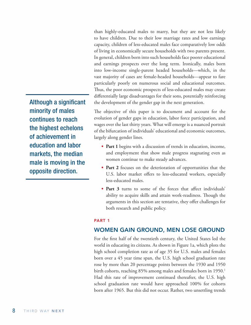
WOMEN GAIN GROUND, MEN LOSE GROUNDFor the first half of the twentieth century, the United States led the world in educating its citizens. As shown in Figure 1a, which plots the high school completion rate as of age 35 for U.S. males and females born over a 45 year time span, the U.S. high school graduation rate rose by more than 20 percentage points between the 1930 and 1950 birth cohorts, reaching 85% among males and females born in 1950.1 Had this rate of improvement continued thereafter, the U.S. high school graduation rate would have approached 100% for cohorts born after 1965. But this did not occur. Rather, two unsettling trends
9Wayward Sons: The Emerging Gender Gap in Labor Markets and Education
commenced with cohorts born after the late 1940s. The rapid secular improvement in U.S. high school graduation rates slowed dramatically. Simultaneously, a gap opened between the graduation rates of males and females.
Over the space of the next twenty cohorts—those born between 1951 and 1970—female high school graduation rates rose by a mere 5 percentage points while the graduation rate of males rose by half that amount. Looking forward an additional 5 years, the female high school graduation rate remained practically stagnant, exhibiting tangible growth only between 1974 and 1975, when it reached 91% for the 1975 birth cohort. Contemporaneously, the gender gap opened further to 3 percentage points. While the U.S. male high school graduation rate of 88% for the 1975 birth cohort is a substantial improvement relative to three decades earlier, it merely achieves parity with the high school graduation rate of females born in 1955.3 Thus, the gender gap in high school completion—which was virtually non-existent prior to the 1950 birth cohort—became a robust feature of the U.S. educational landscape during the ensuing 25 years.4
Since educational attainment is a cumulative process, one would expect the emerging gender gap in high school completion to yield a
0.60
0.65
0.70
0.75
0.80
0.85
0.90
0.95
Frac
tion
with
Hig
h Sc
hool
Deg
ree
1930 1935 1940 1945 1950 1955 1960 1965 1970 1975
Year of Birth
FemalesMales
Figure 1a: High School Graduation Rates at Age 35: U.S. Males and Females Born 1930-19752
Source: Census IPUMS 1 percent samples for years 1960 and 1970, Census IPUMS 5 percent samples for years 1980, 1990, and 2000 and American Community Survey (ACS) 2010.

10 T H I R D W AY N E X T
corresponding gender gap in college attendance and completion. In actuality, something far more dramatic occurred.
As with high school graduation, Americans born between 1930 and 1950 made remarkable gains in college attendance and completion relative to earlier cohorts: the fraction attending college rose by more than 25 percentage points while the fraction completing rose by approximately 15 percentage points (Figures 1b and 1c). Distinct from high school graduations, however, there was a substantial gender gap in college-going among those born between 1930 and the late 1940s, which in this case favored males.6
Similar to the deceleration seen in the high school graduation rate, this inter-cohort pattern of progress in college-going decelerated sharply among cohorts born after approximately 1946. Unlike the high-school graduation rate, which merely stagnated, male college attendance and college completion rates fell sharply for cohorts born from the late 1940s through the late 1950s. In the same interval, improvements in female college attendance and completion ground to a halt, but they did not reverse course.
When college-going rates again began to rise with cohorts born after the late 1950s, female college attendance and completion rates increased sharply while those of males lagged. Cumulating over twenty-five years, these divergent trends have produced a sizable gulf
0.20
0.25
0.30
0.35
0.40
0.45
0.50
0.55
0.60
0.65
0.70
Frac
tion
Atte
ndin
g An
y C
olle
ge
1930 1935 1940 1945 1950 1955 1960 1965 1970 1975
Year of Birth
FemalesMales
Figure 1b: Percent of Adults with Some College Education by Age 355
Source: Census IPUMS 1 percent samples for years 1960 and 1970, Census IPUMS 5 percent samples for years 1980, 1990, and 2000 and American Community Survey (ACS) 2010.
11Wayward Sons: The Emerging Gender Gap in Labor Markets and Education
The remarkable educational progress of females—and the equally stark stagnation of male educational attainment—have profound implications for the welfare of both sexes.
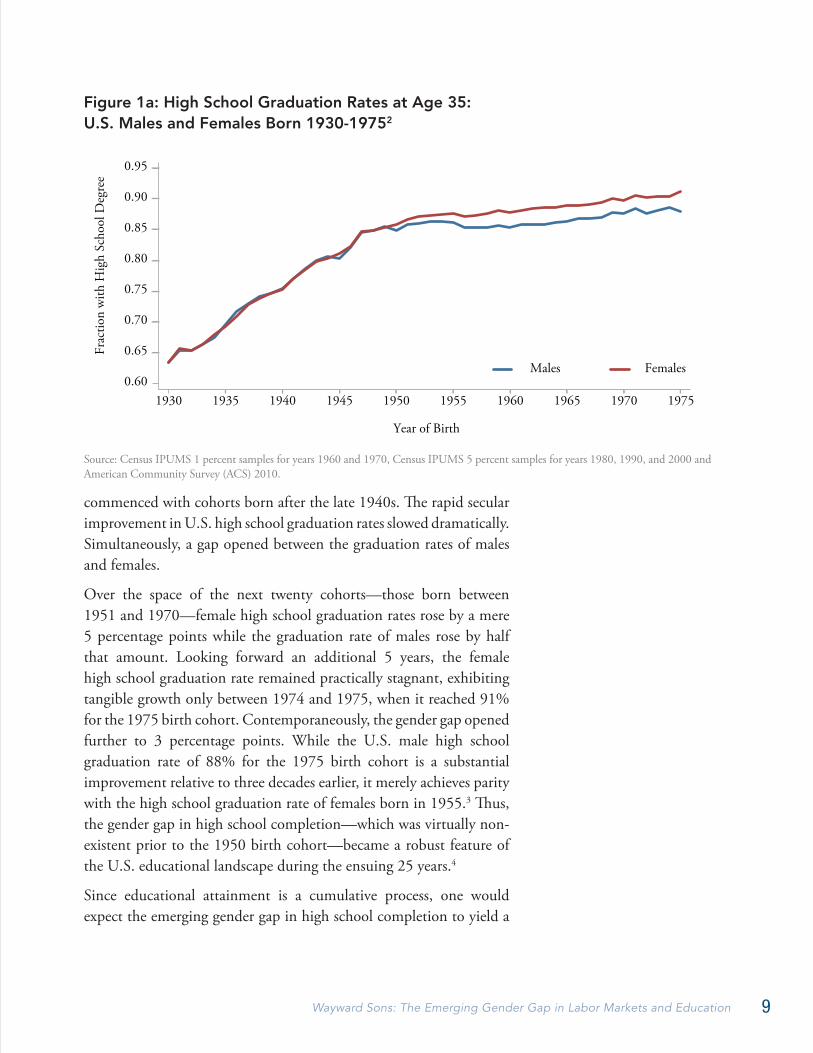
between the college attainment rates of recent cohorts of females and males. Among U.S. adults who were age 35 in 2010 (that is, born in 1975), the female-male gap in college attendance was approximately 10 percentage points, and the gap in four-year college completion was 7 percentage points. Thus, females born in 1975 were roughly 17% more likely than their male counterparts to attend college and nearly 23% more likely to complete a four-year degree. The remarkable educational progress of females—and the equally stark stagnation of male educational attainment—have profound implications for the welfare of both sexes, as we discuss below.
Falling Earnings of Non-College Males
A second dimension along which males have fared poorly in recent decades is earnings. Figure 2 plots changes in real hourly wage levels by sex and education group between 1979 and 2010 for two age groups: ages 25-39 and 40-54.8 The first category corresponds to young prime-age workers, and the latter represents workers in their peak earnings years. This figure highlights two key facts about the evolution of U.S. earnings. First, real earnings growth for U.S. males has been remarkably weak. For males with less than a four-year college education, earnings fell in real terms, declining between 5% and 25%. The steepest falls are found among the least-educated and youngest males, in particular, males under age 40 with high school or lower
0.05
0.10
0.15
0.20
0.25
0.30
0.35
0.40
Frac
tion
With
Col
lege
Deg
ree
1930 1935 1940 1945 1950 1955 1960 1965 1970 1975
Year of Birth
FemalesMales
Figure 1c: Percent of Adults with Four-Year College Degree by Age 357
Source: Census IPUMS 1 percent samples for years 1960 and 1970, Census IPUMS 5 percent samples for years 1980, 1990, and 2000 and American Community Survey (ACS) 2010.

12 T H I R D W AY N E X T
education. Only among males with four or more years of college education do we see real earnings growth in this 30-year period.
Equally apparent from the figure is that the earnings trajectory of U.S. women has been far more propitious. Females have fared better than males in every educational category, and highly educated women have made especially sharp gains in earnings. While real earnings gains among women without any college education have been modest—especially for younger workers—the trends are at least weakly positive for seven of eight female demographics (the exception being young, high-school dropout females).10
Polarizing Occupational Stature
Alongside education and earnings, another measure of workers’ labor market standing is their occupation. While some occupations offer comparatively steep earnings trajectories and a reasonable degree of employment stability, others typically provide limited opportunities for earnings advancement and tenuous employment security. By charting the movement of gender, age, and education groups amongst these occupational categories over time, we can roughly assess whether demographic groups are obtaining employment that offers strong
−25−20−15−10−505
101520253035
−25−20−15−10−505
101520253035
Ages 25−39 Ages 40−64
< High School
HighSchoolGrad
SomeCollege
CollegeGrad
Post-College
< High School
HighSchoolGrad
SomeCollege
CollegeGrad
Post-College
FemalesMales
Figure 2: Percent Changes in Real Hourly Wage Levels 1979-2010 (By Education and Sex)9
Source: May/Outgoing Rotation Groups Current Population Survey data for years 1979-2010.
13Wayward Sons: The Emerging Gender Gap in Labor Markets and Education
career prospects or, conversely, are moving along more precarious employment pathways.
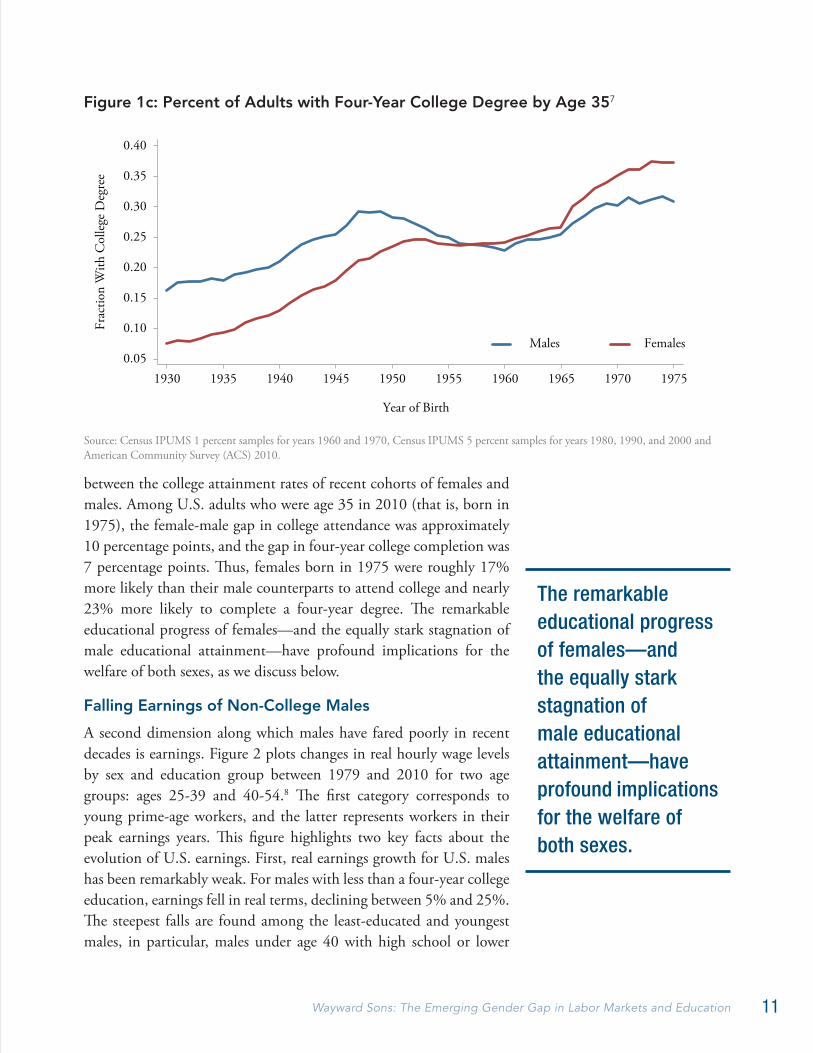
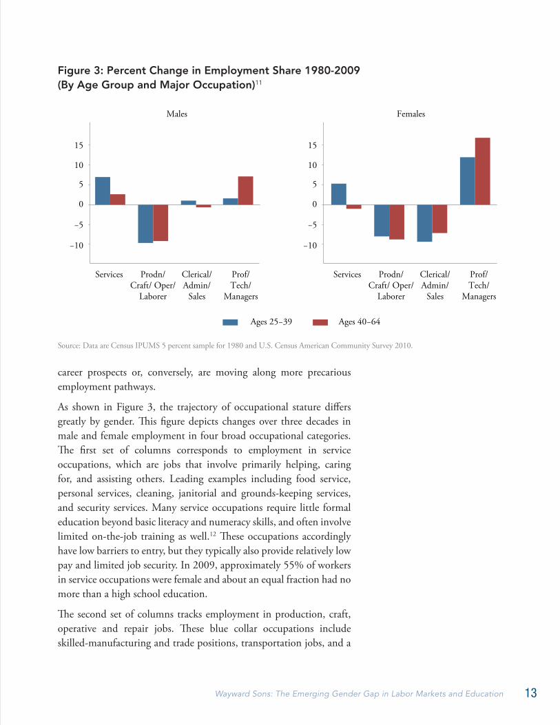
As shown in Figure 3, the trajectory of occupational stature differs greatly by gender. This figure depicts changes over three decades in male and female employment in four broad occupational categories. The first set of columns corresponds to employment in service occupations, which are jobs that involve primarily helping, caring for, and assisting others. Leading examples including food service, personal services, cleaning, janitorial and grounds-keeping services, and security services. Many service occupations require little formal education beyond basic literacy and numeracy skills, and often involve limited on-the-job training as well.12 These occupations accordingly have low barriers to entry, but they typically also provide relatively low pay and limited job security. In 2009, approximately 55% of workers in service occupations were female and about an equal fraction had no more than a high school education.
The second set of columns tracks employment in production, craft, operative and repair jobs. These blue collar occupations include skilled-manufacturing and trade positions, transportation jobs, and a
−10
−5
0
5
10
15
−10
−5
0
5
10
15
Males Females
Services Prodn/ Craft/ Oper/
Laborer
Clerical/ Admin/
Sales
Prof/ Tech/
Managers
Services Prodn/ Craft/ Oper/
Laborer
Clerical/ Admin/
Sales
Prof/ Tech/
Managers
Ages 40−64Ages 25−39
Figure 3: Percent Change in Employment Share 1980-2009 (By Age Group and Major Occupation)11
Source: Data are Census IPUMS 5 percent sample for 1980 and U.S. Census American Community Survey 2010.

14 T H I R D W AY N E X T
variety of less-skilled manual labor intensive jobs. Wages are generally higher in these positions than in service occupations. Traditionally, these jobs have been the province of non-college males, and even in 2009, approximately 85% of workers in these occupations were males and more than 60% had high school or lower education. Nevertheless, training and career advancement opportunities are typically greater in these blue-collar positions than in service occupations, and hence many economists would broadly classify this set of occupations as providing middle-skill and middle-wage positions.
The third set of columns depicts employment growth in clerical, administrative support, and sales occupations. Analogous to the blue-collar positions above, clerical, administrative support, and sales occupations have typically served as the middle-skill, middle-wage positions held by females without a four-year college degree. As of 2009, almost 65% of workers in these occupations were female, approximately 35% had high-school or lower education, and another 45% had some college but no degree.
The final set of columns corresponds to managerial, professional, and technical occupations, which are highly-educated and highly-paid. In 2009, more than 60% of workers in these occupations had at least a four-year college degree, and more than one quarter had graduate or professional education as well. A slight majority (52%) of workers in managerial, professional, and technical occupations were female in 2009.
A central pattern evident in Figure 3 is that there has been a substantial decline in middle-skill employment among both sexes. The share of male and female workers employed in production, operative, and laborer positions fell by 8 to 10 percentage points between 1980 and 2009. Simultaneously, females experienced an equally large fall in clerical, administrative support, and sales employment.13 The declining share of employment in these occupations reflects in large part the ongoing automation and offshoring of so-called ‘routine tasks’—job activities that are sufficiently well defined that they can be carried out successfully by a computer executing a program or by a comparatively less-educated worker overseas who carries out the task with minimal discretion.14 While the pattern of declining employment in routine task-intensive middle-skill jobs has been widely documented across industrialized countries,15 it is less frequently noted that this pattern is particularly pronounced for female workers.16
15Wayward Sons: The Emerging Gender Gap in Labor Markets and Education
The dramatic fall in female employment in routine task-intensive, middle-skill, middle-wage jobs might be expected to augur ill for the employment prospects of females over these three decades. Yet the right-hand panel of Figure 3 indicates otherwise. The very sharp declines in female employment in middle-skill jobs have been substantially offset by rising female employment in high-skill professional, technical, and managerial jobs. Among female workers under age 40, approximately two-thirds of the decline at the middle has been offset by rising employment in high-wage occupations. And among women ages 40 and above, employment gains in high-skill occupations are even larger than employment losses at the middle.
Figure 3 reveals, however, that men have adapted to this new labor market less successfully than women. Among younger males, almost the entirety of declining employment in traditional blue-collar occupations is offset by a rise of male employment in service occupations; gains by young males in professional, technical, and managerial occupations are less than one-quarter as large as their gains in service occupation employment. Among older males ages 40 and above, the pattern is more favorable but still substantially lags that of females. About two-thirds of the loss in middle-skill employment by older males is offset by rising employment in professional, technical, and managerial occupations; this stands in contrast to the more than full offset among females of the same age groups.
Declining Male Employment Rates
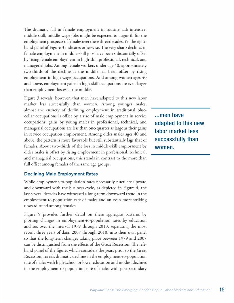
While employment-to-population rates necessarily fluctuate upward and downward with the business cycle, as depicted in Figure 4, the last several decades have witnessed a long-term downward trend in the employment-to-population rate of males and an even more striking upward trend among females.
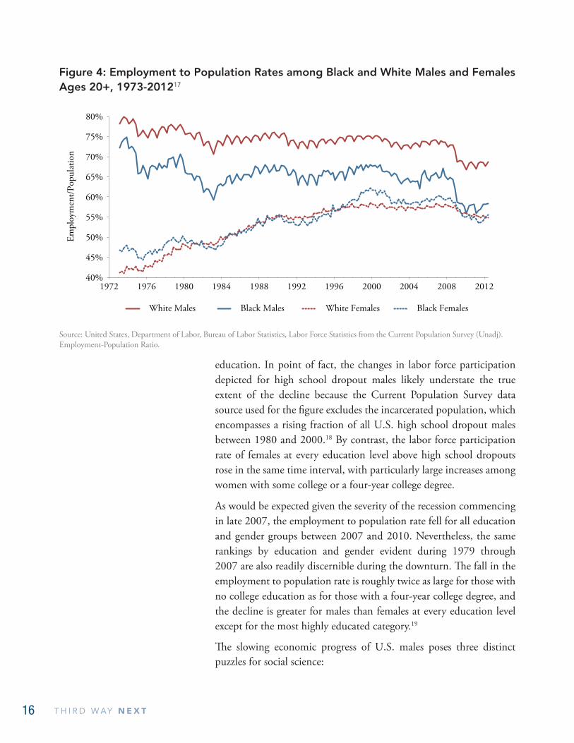
Figure 5 provides further detail on these aggregate patterns by plotting changes in employment-to-population rates by education and sex over the interval 1979 through 2010, separating the most recent three years of data, 2007 through 2010, into their own panel so that the long-term changes taking place between 1979 and 2007 can be distinguished from the effects of the Great Recession. The left-hand panel of the figure, which considers the years prior to the Great Recession, reveals dramatic declines in the employment-to-population rate of males with high-school or lower education and modest declines in the employment-to-population rate of males with post-secondary
...men have adapted to this new labor market less successfully than women.
16 T H I R D W AY N E X T
education. In point of fact, the changes in labor force participation depicted for high school dropout males likely understate the true extent of the decline because the Current Population Survey data source used for the figure excludes the incarcerated population, which encompasses a rising fraction of all U.S. high school dropout males between 1980 and 2000.18 By contrast, the labor force participation rate of females at every education level above high school dropouts rose in the same time interval, with particularly large increases among women with some college or a four-year college degree.
As would be expected given the severity of the recession commencing in late 2007, the employment to population rate fell for all education and gender groups between 2007 and 2010. Nevertheless, the same rankings by education and gender evident during 1979 through 2007 are also readily discernible during the downturn. The fall in the employment to population rate is roughly twice as large for those with no college education as for those with a four-year college degree, and the decline is greater for males than females at every education level except for the most highly educated category.19
The slowing economic progress of U.S. males poses three distinct puzzles for social science:
40%
45%
50%
55%
60%
65%
70%
75%
80%
1972 1976 1980 1984 1988 1992 1996 2000 2004 2008 2012
Empl
oym
ent/P
opul
atio
n
White Males Black Males White Females Black Females
Figure 4: Employment to Population Rates among Black and White Males and Females Ages 20+, 1973-201217
Source: United States, Department of Labor, Bureau of Labor Statistics, Labor Force Statistics from the Current Population Survey (Unadj). Employment-Population Ratio.
17Wayward Sons: The Emerging Gender Gap in Labor Markets and Education
• A first is why male educational attainment has slowed dramatically over the last four decades even as college-going and four-year college attainment among women of the same cohorts has surged.
• A second is why the labor force participation rates of non-college males have declined.
• A third is why the real earnings of non-college males have fallen, both in absolute terms and relative to females of the same age and education levels. While the slackening pace of male educational attainment would be expected to lead to a slowing rate of aggregate male earnings growth, slowing education attainment is clearly not by itself a sufficient explanation for declining earnings within education groups (among non-college males in particular).
We focus on these labor market puzzles in this section of the paper, beginning with the declining employment rates of non-college males and subsequently turning to the evolution of wages. We then widen our frame further to examine socioeconomic forces that may explain why male educational attainment has lagged.
−0.10
−0.05
0.00
0.05
0.10
0.151979−2007 2007−2010
< High School
HighSchoolGrad
SomeCollege
CollegeGrad
Post-College
< High School
HighSchoolGrad
SomeCollege
CollegeGrad
Post-College
Perc
enta
ge P
oint
Cha
nge
in
Empl
oym
ent t
o Po
pula
tion
Rat
e
−0.10
−0.05
0.00
0.05
0.10
0.15
Perc
enta
ge P
oint
Cha
nge
in
Empl
oym
ent t
o Po
pula
tion
Rat
e
FemalesMales
Figure 5: Changes in Employment to Population Rates by Sex and Education Group: Ages 25-64 (1979-2007 and 2007-2010)20
Source: May/Outgoing Rotation Groups Current Population Survey data for years 1979-2010.

18 T H I R D W AY N E X T
PART 2
WHAT HAS GONE WRONG IN THE LABOR MARKET FOR NON-COLLEGE MALES?
Declining Male Labor Force Participation and Declining Opportunity
While the declining employment-to-population rate of less educated workers would appear to be unambiguously bad news, the normative interpretation of this phenomenon depends in large part on whether these employment changes are driven by supply shifts or by demand shifts—that is, by increased desire for leisure by potential workers (a labor supply shift) or by reduced demand for labor by potential employers (a labor demand shift). A straightforward “Economics 101” test to differentiate these explanations is to assess whether a fall in employment for a demographic group is accompanied by a rise in its wages—which would occur if the group had chosen to reduce its labor supply—or whether instead a fall in employment for a demographic group is accompanied by a fall in its wages, which would occur if employer demand for that group’s skills had declined.
We implement this test by calculating the change in each decade in the employment-to-population ratio and average real hourly wage (expressed in logarithms) of 80 demographic groups, as defined by two sexes (male/female), three race categories (white, black, non-white other), four age groups (16-to-24, 25-to-39, 40-to-54, and 55-to- 64), and five education groups (high school dropout, high school graduate, some college, college graduate, and greater than college). The change in the employment-to-population rate over the respective time period is then regressed on the change in the mean logarithmic hourly wage over the same time period. Details of these regressions are relegated to Appendix Tables 1 and 2.
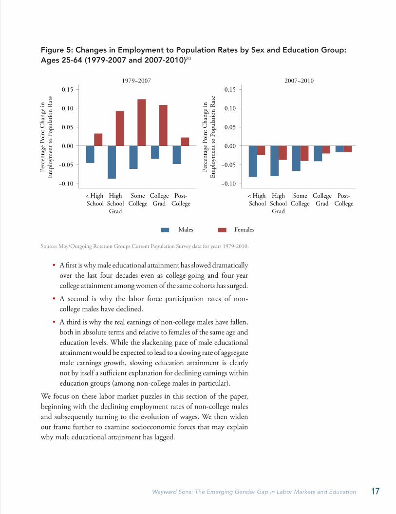
A summary conclusion may be gleaned from Figure 6, which plots changes in employment-to-population rates between 1979 and 2008 among males ages 25 through 39 by race and education group against changes in real hourly wages among these same groups. What this figure reveals is that employment rates have fallen by substantially more for demographic groups that have seen the largest fall in wages over the last three decades. Stated differently, changing real earnings and changing employment-to-population rate are strongly and significantly positively correlated.21 Although not shown in the figure, this positive correlation between rising (or falling) wages and rising (or falling) labor supply
...to understand the decline in labor force participation of less-educated males, we need to understand their declining earnings.
19Wayward Sons: The Emerging Gender Gap in Labor Markets and Education
holds in each of the last three decades (1979-89, 1989-99, and 2000-10), as well as before and during the Great Recession (2000-2007 and 2007-2010). Over the entire 1979-2010 period, a 10% rise in wages for a demographic group is robustly associated with a 5.7 percentage point rise in its employment to population rate. Conversely, a 10% decline in wages is associated with a 5.7 percentage point decline in employment to population. Appendix Table 2 further shows that this robust positive relationship between wage and employment changes is detected for all demographic subgroups: both sexes, all race groups, both younger and older workers, and both college and non-college workers. Demographic groups with declining earnings over the past three decades experienced declining employment-to-population rates, and vice versa for groups with rising earnings.23
This summary evidence strongly supports the view that the changing patterns of employment and earnings documented above are driven to a substantial extent by changes in employers’ demands for workers of various skill levels and occupational specialties, rather than by changes in the supply of workers to the labor market. Thus, to understand the decline in labor force participation of less-educated males, we need to understand their declining earnings.
Figure 6: Relationship between Male Employment to Population Rates and Male Earnings for Persons Ages 25-39, 1979-200822
W SMCW CLG
W GTC
B HSD
B HSG
B SMC
B CLG
B GTC
O HSD
O HSG
O SMC
O CLG
O GTC
−30
−25
−20
−15
−10
−5
0
5
10
W HSG
Perc
enta
ge P
oint
Cha
nge
in
Mal
e Em
ploy
men
t to
Popu
latio
n R
ates
−25 −20 −15 −10 −5 0 5 10 15 20 25 30 35 40
Percentage Change in Male Hourly Wages
Fitted ValuesBlackOther Non−WhiteWhite
W HSD
Source: Census IPUMS 5 percent samples for years 1980, 1990, and 2000 and American Community Survey (ACS) 2009.
20 T H I R D W AY N E X T
The Puzzling Decline in Male Earnings
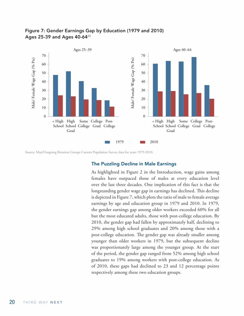
As highlighted in Figure 2 in the Introduction, wage gains among females have outpaced those of males at every education level over the last three decades. One implication of this fact is that the longstanding gender wage gap in earnings has declined. This decline is depicted in Figure 7, which plots the ratio of male to female average earnings by age and education group in 1979 and 2010. In 1979, the gender earnings gap among older workers exceeded 60% for all but the most educated adults, those with post-college education. By 2010, the gender gap had fallen by approximately half, declining to 29% among high school graduates and 20% among those with a post-college education. The gender gap was already smaller among younger than older workers in 1979, but the subsequent decline was proportionately large among the younger group. At the start of the period, the gender gap ranged from 52% among high school graduates to 19% among workers with post-college education. As of 2010, these gaps had declined to 23 and 12 percentage points respectively among these two education groups.
0
10
20
30
40
50
60
70
Mal
e/ F
emal
e W
age
Gap
(% P
ts)
0
10
20
30
40
50
60
70
Mal
e/ F
emal
e W
age
Gap
(% P
ts)
Ages 25−39 Ages 40−64
< High School
HighSchoolGrad
SomeCollege
CollegeGrad
Post-College
< High School
HighSchoolGrad
SomeCollege
CollegeGrad
Post-College
20101979
Figure 7: Gender Earnings Gap by Education (1979 and 2010) Ages 25-39 and Ages 40-6424
Source: May/Outgoing Rotation Groups Current Population Survey data for years 1979-2010.
21Wayward Sons: The Emerging Gender Gap in Labor Markets and Education
This remarkable decline in the gender earnings gap is to a substantial extent an indication of progress, reflecting an increase in the skills and labor market experience of female workers as they have entered professional, managerial, and technical fields and reduced their concentration in traditionally female-dominated occupations such as teaching and nursing.25 But the story is not exclusively about women’s advances. It also reflects male declines. As Figure 2 highlights, the closing of the gender gap among non-college workers is at least as much due to the falling wages of non-college males as it is due to the rising earnings of non-college females. These real earnings declines have had significant adverse consequences, spurring substantial falls in male labor force participation and potentially additional social costs discussed below. Understanding why male wages have fallen may help to interpret the changing opportunity sets faced by male and female workers.
To a surprising extent, however, the causal forces responsible for the sharp wage declines for low education males–and, more generally, the differential patterns of wage growth by education level—are challenging to pin down. Consider, for example, the following hypotheses:
• Wages of low-education males may have fallen while those of low-education females have risen because, within education groups, males have moved into lower-paying occupations while females have moved into higher-paying occupations. Indeed, this explanation is strongly suggested by Figure 3, which documents declining male employment in middle-skill production and operative positions and rising male employment in low-paid service occupations. Surprisingly, the data find that these occupational shifts explain only a minority of the fall in male wages or the rise in female wages. For both males and females, the bulk of the observed changes in wages by education group during this three decade period is proximately explained by changing wages within broad occupational categories rather than movements of employment across categories. Although it is certainly correct that the rising share of non-college male employment found in low-paying service occupations has contributed to declining non-college male wages, this typically explains less than 20% of the decline in non-college male wages, with the remainder due to wage changes within occupations.26
• This observation raises a second possibility: if males are over-represented in occupations with falling wages and females are
This remarkable decline in the gender earnings gap...is not exclusively about women’s advances. It also reflects male declines.

22 T H I R D W AY N E X T
similarly overrepresented in occupations with rising wages, then the gender earnings gap would contract even with no change in the set of occupations in which males and females are employed. Notably, this conjecture also finds at best modest support in the data. For example, between 1983 and 2010, the wage gap between male and female high school dropouts closed by 18.5 percentage points. Of this closure, 15 percentage points was due to falling male wages and 3.5 points to rising female wages. Some simple calculations using gender wage changes by occupation reveal that 75% of shrinkage of the gap was due to rising female relative to male wages within major occupations and only 25% due to male overrepresentation in occupations with falling overall wages. A similar pattern holds at every education level: the substantial closing of the gender gap in each educational category is almost entirely accounted for by rising female relative to male wages within broad occupation groups.27
In short, simple shifts in occupational structure are insufficient to explain the puzzle of declining real wages of non-college males in the U.S. during the last three decades. In reality, there is no single, widely accepted explanation for this phenomenon. A rich and rigorous literature in labor economics has, however, drawn attention to the confluence of three primary forces. A first is rapid and ongoing skill-biased technological change in the U.S. and other advanced countries, which has generally raised demand for highly-educated workers and reduced demand for non-college workers. Rapid improvements in information technology have raised the value of analytical, problem-solving, and managerial skills, leading to rising demand for college-educated workers. Simultaneously, the automation of routine, codifiable tasks has displaced employment in occupations that are intensive in such tasks, most particularly production, operative, clerical, administrative support, and sales jobs. Among non-college males, this force has particularly reduced demand in blue-collar production positions. But as noted above, the decline in middle-skill employment has been even larger among women than men, so declines in middle-skill jobs cannot be the primary explanation for why non-college male wages have fallen as female wages have risen.28
A second significant factor impinging on the earnings of non-college males is the decline in the penetration and bargaining power of labor unions in the United States. Labor unions have historically obtained relatively generous wage and benefit packages for blue-collar workers. Over the last three decades, however, U.S. private-sector union
In short, simple shifts in occupational structure are insufficient to explain the puzzle of declining real wages of non-college males in the U.S. during the last three decades.

23Wayward Sons: The Emerging Gender Gap in Labor Markets and Education
density—that is, the fraction of private-sector workers who belong to labor unions—has fallen by approximately 70%, from 24.2% in 1973 to 16.5% in 1983 to 11.1% in 1993 to 7.5% in 2007, and to 6.9% in 2011.29 While the precise contribution of declining unionization to the evolution of male wage levels and wage inequality is a subject of ongoing debate, a number of studies place this contribution at 20% to 30%.30 Notably, because union membership has been historically quite concentrated among blue-collar workers, the majority of whom are males, the decline in union membership may have differentially affected non-college male earnings.
A third prominent factor is the globalization of labor markets, seen particularly in the greatly increased U.S. trade integration with developing countries. Globalization has become particularly important for U.S. labor markets since the early 1990s when China began its extremely rapid integration into the world trading system. Between 1987 and 2007, the share of total U.S. spending on Chinese goods rose from under one-half of one percent to close to five percent.31 While the influx of Chinese goods lowered consumer prices,32 it also fomented a substantial decline in U.S. manufacturing employment, contributing directly to the decline in production worker employment.33
Notably, these three forces—technological change, deunionization, and globalization—work in tandem. Advances in information and communications technologies have directly changed job demands in U.S. workplaces while simultaneously facilitating the globalization of production by making it increasingly feasible and cost-effective for firms to source, monitor and coordinate complex production processes at disparate locations worldwide. The globalization of production has in turn increased competitive conditions for U.S. manufacturers and U.S. workers, eroding employment at unionized establishments and decreasing the capability of unions to negotiate favorable contracts, attract new members, and penetrate new establishments. 34
In recent years, researchers have also begun to take seriously the possibility that technological and organizational changes in the workplace have differentially raised the productivity, demand for, and earnings levels of women relative to men. Research in this vein posits that women disproportionately possess the combination of cognitive and interpersonal skills that is particularly valuable in information and technology-rich work environments—settings in which the importance of physically demanding and repetitive tasks has been greatly diminished.35 While this hypothesis is, to date, less established
Notably, these three forces—technological change, deunionization, and globalization—work in tandem.

24 T H I R D W AY N E X T
than the three above, some intriguing evidence lends it credibility. At an aggregate level, economists have long noted that the rapid narrowing of the gender gap in earnings over the last three decades has closely coincided with the rising return to higher education.36 This correlation need not be causal, but a recent study by Beaudry and Lewis offers more persuasive evidence, demonstrating that the aggregate relationship between the rising skill premium and the falling gender gaps is evident at the geographic level as well. Specifically, U.S. cities that saw the largest increase in the college/high-school earnings premium between 1980 and 2000 also exhibited a differentially large decline in the male-female wage differential.37 While these suggestive findings are far from the last word on the subject, they lend initial credibility to the hypothesis that the declining real wages of non-college males are in part driven by the same demand-side forces that have raised the premium to college education and narrowed the gender gap.
Does College Pay for Young Males?
The multiple strands of explanation offered above for the declining wages of non-college males—technological change, globalization, and deunionization—are similar on one key dimension: all imply that males have a great deal to gain from post-secondary education. This inference, however, takes as a given that the benefits of higher education exceed the costs. This assumption merits a reality check. Indeed, one natural hypothesis for why male educational attainment might have stagnated in the last three decades is that the return to education for males is simply inadequate to justify its cost. Since female educational attainment has surged during the same period, this argument would further imply that the return to education must be higher—or have risen by more—among females than males. Do the data support this hypothesis?
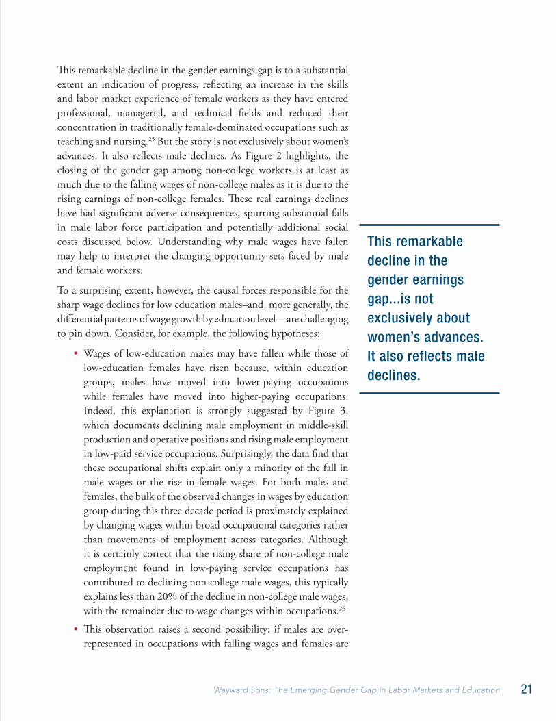
The answer is a resounding no. While wage levels of low-education males have fallen in real terms over the past three decades, the earnings differential between more and less-educated males has increased steeply since the late 1970s, as is visible in Figure 8. For example, among males ages 25 through 39, the earnings differential between four-year college graduates and high school graduates rose from approximately 18 percentage points in 1979 to 51 percentage points in 2010. While in 1979, the college/high-school differential among young females ages 25 through 39 was substantially higher than among males (32% vs. 18%), the 22 percentage point increase in the college/high-school
...the college premium is higher at present than it has been at any time since 1915...
25Wayward Sons: The Emerging Gender Gap in Labor Markets and Education
earnings differential among females was one-third smaller than the 31 percentage point increase among males.39 Moreover, longer historical evidence suggests that the college premium is higher at present than it has been at any time since 1915, when the first representative data on U.S. earnings by education group became available.40
Notably, these dramatic increases in the premium to college education translate into substantial differential gains in lifetime earnings for college graduates versus non-graduates. A recent analysis by Avery and Turner41 estimates that between 1979 and 2010, the present discounted value of a four-year college degree net of tuition costs rose by more than $300 thousand for men and more than $250 thousand for women.42 Thus, ironically, even as male college-going has stagnated and female college-going has soared, the payoff to a four-year college education has risen even more steeply for men than for women.
One might, however, object that although the college degree has become relatively more valuable since 1979, a substantial part of the relative increase—at least for males—stems from the falling wages of non-college workers rather than rising wages of college workers. Is it possible that despite their relative gains, college educated males
−30
−15
0
15
30
45
60
75
90Males Females
< High School/HS Grad
SomeCollege/HS Grad
CollegeGrad/
HS Grad
Post-College/HS Grad
< High School/HS Grad
SomeCollege/HS Grad
CollegeGrad/
HS Grad
Post-College/HS Grad
20101979
Wag
e G
ap R
elat
ive
to H
igh
Scho
ol G
radu
ates
(% p
ts)
−30
−15
0
15
30
45
60
75
90
Wag
e G
ap R
elat
ive
to H
igh
Scho
ol G
radu
ates
(% p
ts)
Figure 8: Educational Wage Differentials by Gender: 1979 and 2010 (Ages 25-39, Males and Females)38
Source: May/Outgoing Rotation Groups Current Population Survey data for years 1979-2010.
26 T H I R D W AY N E X T
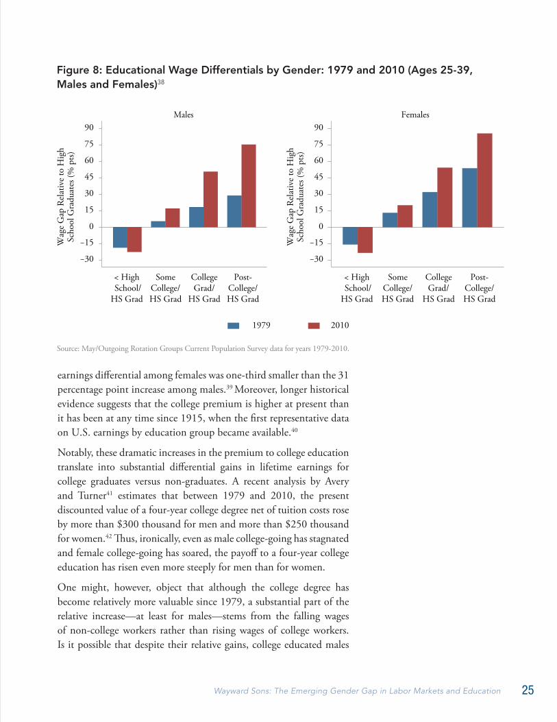
nevertheless do not earn decent wages? Again, the answer is no. Comparing real hourly wage levels among education and sex groups in 2010 (Figure 9) reveals a potentially surprising fact: despite the dramatic relative gains in female earnings, males continue to receive higher average hourly wages at every education level. Among young four year college graduates, males earn an average of $24.30 per hour versus $20.50 among females. Among 25 to 39 year old high school graduates with no college, males averaged $14.70 per hour in 2010 versus $11.90 among females.44
In summary, the opportunities that the U.S. labor market offers to less-educated workers, particularly less-educated males, have deteriorated substantially in the past thirty years. In the same period, the real earnings of college males and females have significantly improved, even accounting for the rising tuition cost of a four-year college education. The economic case for the four-year college degree for young U.S. adults—both male and female—has probably never been stronger. Seen in this light, the flagging college attainment of U.S. males is all the more puzzling.
0
5
10
15
20
25
30
35
40
0
5
10
15
20
25
30
35
40Ages 25−39 Ages 40−64
< High School
HighSchoolGrad
SomeCollege
CollegeGrad
Post-College
< High School
HighSchoolGrad
SomeCollege
CollegeGrad
Post-College
FemalesMales
Figure 9: Geometric Mean Real Hourly Wage Levels in 2010, By Education and Sex, Ages 25-39 and Ages 40-6443
Source: May/Outgoing Rotation Groups Current Population Survey data for years 1979-2010.
27Wayward Sons: The Emerging Gender Gap in Labor Markets and Education
PART 3
CHANGING FAMILY STRUCTURE AND THE EMERGING GENDER GAP
We now turn our attention from the labor market to ‘pre-market’ factors that may contribute to the emerging gender gaps documented above. By ‘pre-market,’ we mean factors that affect individuals’ skills acquisition and work-preparedness prior to the age of labor market entry. We offer two interdependent hypotheses that may help to explain why the gender gap has emerged. The first part of the hypothesis concerns the impact of changing economic opportunities for males and females on family structure. The second part concerns the impact of changing family structure on the educational attainment of children, particularly young males.
To preview, we argue first that sharp declines in the earnings power of non-college males combined with gains in the economic self-sufficiency of women—rising educational attainment, a falling gender gap, and greater female control over fertility choices—have reduced the economic value of marriage for women. This has catalyzed a sharp decline in the marriage rates of non-college U.S. adults—both in absolute terms and relative to college-educated adults—a steep rise in the fraction of U.S. children born out of wedlock, and a commensurate growth in the fraction of children reared in households characterized by absent fathers.
The second part of the hypothesis posits that the increased prevalence of single-headed households and the diminished child-rearing role played by stable male parents may serve to reinforce the emerging gender gaps in education and labor force participation by negatively affecting male children in particular. Specifically, we review evidence that suggests that male children raised in single-parent households tend to fare particularly poorly, with effects apparent in almost all academic and economic outcomes. One reason why single-headedness may affect male children more and differently than female children is that the vast majority of single-headed households are female-headed households. Thus, boys raised in these households are less likely to have a positive or stable same-sex role model present. Moreover, male and female children reared in female-headed households may form divergent expectations about their own roles in adulthood—with girls
...increased prevalence of single-headed households and the diminished child-rearing role played by stable male parents may serve to reinforce the emerging gender gaps in education.

28 T H I R D W AY N E X T
anticipating assuming primary childrearing and primary income-earning responsibilities in adulthood and boys anticipating assuming a secondary role in both domains. We next review the evidence bearing on these hypotheses.*
Changes in Family Structure: The Declining Value of Marriage
Arguably, the most salient change in the U.S. family structure over the past forty years has been the substantial decline in the prevalence of marriage. This decline is charted in Figure 10, which plots the fraction of young men and women ages 25-39 who are currently married at the start of each decade between 1970 and 2010. Though the downward trend is apparent in every sub-group, the magnitude of the change is largest for blacks and the least educated, and smallest for Hispanics and those with at least some college education.45 In 1970, 57% of black women with less than a high school diploma were married. By 2010, this number had plummeted to 18%. We observe an even sharper decline among black men: in 1970, 69% of black men with less than a high school diploma were married; in 2010, only 17% were married.46
In considering these figures, it is critical to bear in mind that individuals tend to cohabit and marry disproportionately within their own education and race groups (which social scientists term ‘assortative mating’), and this tendency has strengthened over time. For example, in 1970, approximately 40% of the spouses of four-year college graduate males ages 30 through 44 were themselves college graduates—a fraction that substantially exceeded the fraction of adult women who were college graduates in that year. In the ensuing decade, this association strengthened. By 2007, the fraction of spouses of four-year college males in the 30 through 44 age bracket who were also college graduates had risen to over 70%.47
Given the importance of assortative mating, the diminished capacity of non-college males to earn a salary sufficient to support a family would be expected to differentially reduce the value of marriage—and
* Our discussion above focuses on heterosexual household relationships since available studies do not offer detailed information on children in same-sex marriages. Future research will add to our knowledge of children’s outcomes in same-sex marriages, but initial research shows that children raised by two same-sex parents have similar psychological outcomes to those raised by male and female two-parent households (see endnote 75 for full source).
...the most salient change in the U.S. family structure over the past forty years has been the substantial decline in the prevalence of marriage.

29Wayward Sons: The Emerging Gender Gap in Labor Markets and Education
hence the marriage rate—for non-college women. This hypothesis finds support in Figure 10. What is particularly interesting in the figure is that, within race groups, marriage rates were initially similar among all education levels in 1970, and then diverged thereafter. As detailed above, though less-educated men have experienced a reduction in real wages, women of almost all education levels have made advances. That the least educated males and females have experienced the most rapid decline in marriage rates during a time of increasing returns for education and real wage declines among less-educated men provides suggestive evidence that the economic benefits of marriage have declined, particularly for less-educated women.48
One may gain further insight into the economic determinants of marriage by plotting changes in marriage rates among young women
White Men Black Men Hispanic Men
.2
.3
.4
.5
.6
.7
.8
.9
.2
.3
.4
.5
.6
.7
.8
.9
.2
.3
.4
.5
.6
.7
.8
.9
.2
.3
.4
.5
.6
.7
.8
.9
.2
.3
.4
.5
.6
.7
.8
.9
.2
.3
.4
.5
.6
.7
.8
.9
Year
White Women
Year
Black Women
Year
Hispanic Women
Less �an H.S. High School More than H.S.
1970 1980 1990 2000 2010 1970 1980 1990 2000 2010 1970 1980 1990 2000 2010
Year Year Year1970 1980 1990 2000 2010 1970 1980 1990 2000 2010 1970 1980 1990 2000 2010
Figure 10: Marriage Rate of Young Men and Women, By Race and Education, Ages 25-39, 1970-2010, White Men, Black Men, Hispanic Men, White Women, Black Women, and Hispanic Women49
Source: Census IPUMS 5 percent samples for years 1980, 1990, and 2000 and American Community Survey (ACS) 2010.
30 T H I R D W AY N E X T
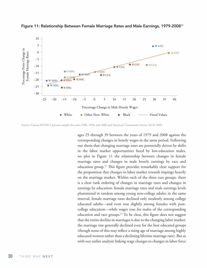
ages 25 through 39 between the years of 1979 and 2008 against the corresponding changes in hourly wages in the same period. Following our thesis that changing marriage rates are potentially driven by shifts in the labor market opportunities faced by low-education males, we plot in Figure 11 the relationship between changes in female marriage rates and changes in male hourly earnings by race and education group.51 This figure provides remarkably clear support for the proposition that changes in labor market rewards impinge heavily on the marriage market. Within each of the three race groups, there is a clear rank ordering of changes in marriage rates and changes in earnings by education: female marriage rates and male earnings levels plummeted in tandem among young non-college adults; in the same interval, female marriage rates declined only modestly among college educated adults—and even rose slightly among females with post-college education—while wages rose for males of the corresponding education and race groups.52 To be clear, this figure does not suggest that the entire decline in marriages is due to the changing labor market; the marriage rate generally declined even for the best educated groups (though some of this may reflect a rising age of marriage among highly educated women rather than a declining lifetime marriage rate). But as with our earlier analysis linking wage changes to changes in labor force
W HSD
W SMC
W CLG
W GTC
B HSD
B HSG
B SMC
B CLG
B GTC
O HSD
O HSG O SMC
O CLG
O GTC
−30
−25
−20
−15
−10
−5
0
5
10
W HSG
Perc
enta
ge P
oint
Cha
nge
in
Fem
ale
Mar
riage
Rat
es
−25 −20 −15 −10 −5 0 5 10 15 20 25 30 35 40
Percentage Change in Male Hourly Wages
Fitted ValuesBlackOther Non−WhiteWhite
Figure 11: Relationship Between Female Marriage Rates and Male Earnings, 1979-200850
Source: Census IPUMS 5 percent samples for years 1980, 1990, and 2000 and American Community Survey (ACS) 2009.

31Wayward Sons: The Emerging Gender Gap in Labor Markets and Education
participation (Figure 6), these data support the view that changes in earnings opportunities by education group have played a central role in reshaping both employment rates and family formation.53
A recent randomized evaluation of Career Academies—a career-oriented high school program that provides small learning communities, emphasis on career paths, and internship opportunities for disadvantaged high school students—lends additional credence to the potential causal link between male earnings capacity and marriage rates. Eight years after students graduated from high school, males who participated in Career Academies due to the experiment were earning on average $361 more per month and were employed almost three months more per year than males who were experimentally assigned to traditional high school programs.54 Equally remarkable were the differences among Career Academy participants and non-participants in measures of family formation: male participants were 33% more likely to be married and living with their spouse, 30% more likely to be living with their partner and children, and 35% more likely to be the custodial parent of their children.55
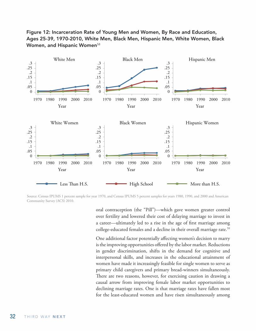
Alongside shifts in earnings capacity, a second force that has likely reduced the set of available males that are of “marriageable quality” is a substantial rise in the male incarceration rate during the last three decades. As documented by Figure 12, less than five percent of black men ages 25 to 39 without a high school degree were in prison in 1970. By 2010, this number had more than quintupled to 26%.56
Evidence of a causal link between male incarceration and female marriage rates comes from research by Charles and Luoh, 2010.57 Utilizing changes in federal and state criminal sentencing laws during the late 1980s and 1990s, which increased criminalization and punishment of drug offenses as part of the “war on drugs,” Charles and Luoh estimate that a 1 percentage point increase in the male incarceration rate reduces the probability that a female ever marries by 1 percentage point. The effect is most pronounced for women without a college degree who, logically, are more likely than college-educated women to marry within the pool of men who are incarcerated.
It is also likely that changes in legal and societal norms that permitted women greater control over fertility decisions have altered the decision to marry. Take, for example, the dramatic rise in age at marriage. For college-educated females born in 1940, a little over 70% were married by age 26. By the 1960 cohort, however, only 50% were married by age 26. There is growing evidence that the expansion of access to
...a second force that has likely reduced the set of available males that are of “marriageable quality” is a substantial rise in the male incarceration rate during the last three decades.
32 T H I R D W AY N E X T
oral contraception (the “Pill”)—which gave women greater control over fertility and lowered their cost of delaying marriage to invest in a career—ultimately led to a rise in the age of first marriage among college-educated females and a decline in their overall marriage rate.59
One additional factor potentially affecting women’s decision to marry is the improving opportunities offered by the labor market. Reductions in gender discrimination, shifts in the demand for cognitive and interpersonal skills, and increases in the educational attainment of women have made it increasingly feasible for single women to serve as primary child caregivers and primary bread-winners simultaneously. There are two reasons, however, for exercising caution in drawing a causal arrow from improving female labor market opportunities to declining marriage rates. One is that marriage rates have fallen most for the least-educated women and have risen simultaneously among
0.05
.1.15
.2.25
.3
0.05
.1.15
.2.25
.3
0.05
.1.15
.2.25
.3
0.05
.1.15
.2.25
.3
0.05
.1.15
.2.25
.3
0.05
.1.15
.2.25
.3
Year Year Year
Less �an H.S. High School More than H.S.
1970 1980 1990 2000 2010 1970 1980 1990 2000 2010 1970 1980 1990 2000 2010
White Men Black Men Hispanic Men
White Women Black Women Hispanic Women
Year Year Year1970 1980 1990 2000 2010 1970 1980 1990 2000 2010 1970 1980 1990 2000 2010
Figure 12: Incarceration Rate of Young Men and Women, By Race and Education, Ages 25-39, 1970-2010, White Men, Black Men, Hispanic Men, White Women, Black Women, and Hispanic Women58
Source: Census IPUMS 1 percent sample for year 1970, and Census IPUMS 5 percent samples for years 1980, 1990, and 2000 and American Community Survey (ACS) 2010.
33Wayward Sons: The Emerging Gender Gap in Labor Markets and Education
college-educated women.60 Since the former group has seen the smallest rise in earnings power and the latter group the largest, a self-sufficiency argument would have predicted precisely the opposite: a greater decline in the marriage rate among college-educated women. Secondly, it is likely that some portion of the increase in women’s education and investment in long-term careers is a symptom rather than a cause of declining marriage rates. As the earnings capacity of low-education males has fallen, women have had little choice but to invest in market skills. Thus, while we are comfortable in crediting part of the decline in marriage rates to the falling earnings power of non-college males, we are less confident in making the same causal claim for rising women’s earnings.
The Rising Prevalence of Men Not Living With Their Children
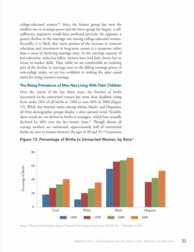
Over the course of the last thirty years, the fraction of births accounted for by unmarried women has more than doubled, rising from under 20% of all births in 1980 to over 40% in 2009 (Figure 13). While this fraction varies among whites, blacks, and Hispanics, all three demographic groups display a clear upward trend. Notably, these trends are not driven by births to teenagers, which have actually declined by 40% over the last twenty years.61 Though almost all teenage mothers are unmarried, approximately half of nonmarital births are now to women between the ages of 20 and 29.62 Consistent
0
20
40
60
80
Perc
enta
ge o
f Birt
hs
Total White Black Hispanic
1980 1990 2000 2009
Figure 13: Percentage of Births to Unmarried Women, by Race63
Source: “National Vital Statistics Report,”National Vital Statistics Data System, Vol. 60, No. 1, November 3, 2011.

34 T H I R D W AY N E X T
with our discussion above on the declining value of marriage, the rise of single parenthood is primarily the result of an increase in never-married women and nonmarital births, not due to higher divorce or widowing rates.65
If traditional marriages were simply giving way to cohabitation, one might infer that declining marriage rates and the concomitant rise in out-of-wedlock births represent a nominal rather than a substantive change in household structures.66 This, however, is not the case: the fraction of women cohabiting with the fathers of their children has fallen considerably. We observe in Figure 14 a sharp decline in the fraction of young men who report living with a related child.67
While approximately 75% of white men with a high school diploma or less were living with a child in 1970, by 2010 only 40% were. On the other hand, 65% of white women with a high school diploma
0
.25
.5
.75
1
0
.25
.5
.75
1
0
.25
.5
.75
1
0
.25
.5
.75
1
0
.25
.5
.75
1
0
.25
.5
.75
1
Year Year Year
Less �an H.S. High School More than H.S.
1970 1980 1990 2000 2010 1970 1980 1990 2000 2010 1970 1980 1990 2000 2010
White Men Black Men Hispanic Men
White Women Black Women Hispanic Women
Year Year Year1970 1980 1990 2000 2010 1970 1980 1990 2000 2010 1970 1980 1990 2000 2010
Figure 14: Fraction of Young Men and Women Reporting at Least One Child at Home, By Race and Education, Ages 25-39, 1970-2010, White Men, Black Men, Hispanic Men, White Women, Black Women, and Hispanic Women64
Source: Census IPUMS 1 percent sample for year 1970, and Census IPUMS 5 percent samples for years 1980, 1990, and 2000 and American Community Survey (ACS) 2010.
35Wayward Sons: The Emerging Gender Gap in Labor Markets and Education
or less were living with a related child in 2010, down from 85% in 1970. While this fall of 20 percentage points is substantial, it is only slightly more than half as large as the fall among white men of the same education level.
These gender differences are even more pronounced among young black men and women: between 1970 and 2010, the fraction of black men with a high school education living with biological children fell from over 65% to approximately 25% —a 60% drop—with an even larger decline among black high school dropout men. Among black women of the same education level, however, the fraction living with biological children declined only slightly, from 75% in 1970 to 65% in 2010. Given the strong patterns of assortative mating by race and education discussed above, it is a near certainty that the sharp fall in the fraction of males living with related children largely reflects a change in cohabitation rates rather than a fall in the fraction of males who have fathered children.69
0.25.5
.751
0.25.5
.751
0.25
.5.75
1
0.25
.5.75
1
1970 1980 1990 2000 2010 1970 1980 1990 2000 2010
All Children White
Black Hispanic
1970 1980 1990 2000 2010 1970 1980 1990 2000 2010
Two Parents Mother Only Father Only No Parents
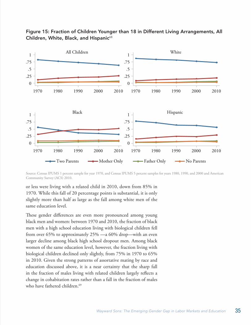
Figure 15: Fraction of Children Younger than 18 in Different Living Arrangements, All Children, White, Black, and Hispanic68
Source: Census IPUMS 1 percent sample for year 1970, and Census IPUMS 5 percent samples for years 1980, 1990, and 2000 and American Community Survey (ACS) 2010.
36 T H I R D W AY N E X T
Figure 15 further supports the view that men have become increasingly absent from the family living arrangements of their related children.70 The figure plots the percentage of children under eighteen who live with two parents (biological, adoptive, or step-parent), their mother only, their father only, or no parent. While 82% of children under eighteen were living with two parents in 1970, this figure had dropped to 63% by 2010. Over the same time period, there was a sharp rise in the percentage of children living with a single parent, from 14% to 33%, with the vast majority of these children living with their mother only.
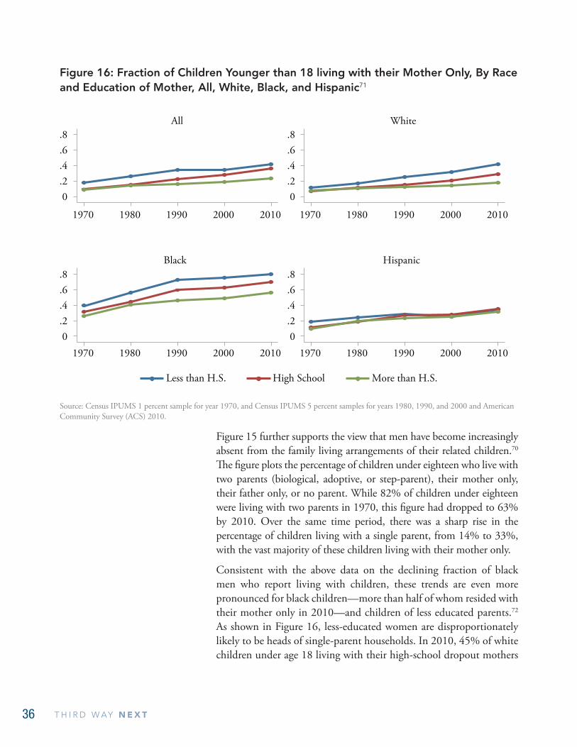
Consistent with the above data on the declining fraction of black men who report living with children, these trends are even more pronounced for black children—more than half of whom resided with their mother only in 2010—and children of less educated parents.72 As shown in Figure 16, less-educated women are disproportionately likely to be heads of single-parent households. In 2010, 45% of white children under age 18 living with their high-school dropout mothers
0.2.4.6.8
0.2.4.6.8
1970 1980 1990 2000 2010 1970 1980 1990 2000 2010
1970 1980 1990 2000 2010 1970 1980 1990 2000 2010
All White
Black Hispanic
Less than H.S. High School More than H.S.
0.2.4.6.8
0.2.4.6.8
Figure 16: Fraction of Children Younger than 18 living with their Mother Only, By Race and Education of Mother, All, White, Black, and Hispanic71
Source: Census IPUMS 1 percent sample for year 1970, and Census IPUMS 5 percent samples for years 1980, 1990, and 2000 and American Community Survey (ACS) 2010.
37Wayward Sons: The Emerging Gender Gap in Labor Markets and Education
were in households where the mother was the only adult. Among black children of the same age, this fraction exceeded 75%.
It would be a misreading of these data, however, to infer that a large fraction of U.S. children are reared in households where no adult male is present. The increasing prevalence of cohabitation, divorce, and remarriage among U.S. households means that many different adult males may be present during the various years of a child’s upbringing. By the same token, the average fraction of years in which the biological father is present is on the wane while the average fraction of years in which no adult male is present is on the rise. The sociologist Andrew Cherlin summarizes these changes eloquently:73
Marriage remains the most common living arrangement for raising children. At any one time, most American children are being raised by two parents. Marriage, however, is less dominant in parents’ and children’s lives than it once was. Children are more likely to experience life in a single-parent family, either because they are born to unmarried mothers or because their parents divorce. And children are more likely to experience instability in their living arrangements as parents form and dissolve marriages and partnerships.
Cherlin further emphasizes the divergence in family structures by class:74
A half-century ago, the family structures of poor and non-poor children were similar: most children lived in two-parent families. In the intervening years, the increase in single-parent families has been greater among the poor and near-poor. Women at all levels of education have been postponing marriage, but less-educated women have postponed childbearing less than better-educated women have. The divorce rate in recent decades appears to have held steady or risen for women without a college education but fallen for college-educated women. As a result, differences in family structure according to social class are much more pronounced than they were fifty years ago... Among the less educated, early childbearing outside of marriage has become more common, as the ideal of finding a stable marriage and then having children has weakened, whereas among the better educated, the strategy is to delay childbearing and marriage until after investing in schooling and careers.
In short, U.S. children born into low-education and minority households spend a substantial and rising share of their childhoods in single-parent, divorced, and remarried households; they are exposed
U.S. children born into low-education minority households...experience a comparatively smaller number of years in which a stable father is present in the household.
38 T H I R D W AY N E X T
to a disproportionate number of adult partner relationships through cohabitation and remarriage among their primary caregivers; and they experience a comparatively smaller number of years in which a stable father is present in the household.75
Inequality of Financial and Parental Resources
The above discussion highlights how the declining economic prospects of non-college men, combined with the anemic growth of male college attainment, have fomented profound changes in the structure of American families over the last forty years. We now consider a feedback mechanism that reverberates in the opposite direction—from changes in family structure to future economic challenges. Specifically, we review evidence that these profound changes in family structure reinforce and exacerbate the divergent educational and economic trends of males and females.
It is widely documented that children of single-parent homes fare worse on a broad range of outcomes relative to children of dual-parent homes. In comparison to children living with both biological parents, children living with a single mother score lower on academic achievement tests, have lower grades, have a higher incidence of behavioral problems, and display a greater tendency to engage in risky behaviors such as drug use and criminal activity.76 Notably, the effects of even relatively short periods of parental absence are detectable in children’s test scores.77
What accounts for these disparities? We focus on two consequences of the rise of single-headed households that are potentially responsible for emerging gender gaps: inequality of financial resources and inequality of parental resources, where by parental resources, we mean non-monetary factors impinging on parents’ ability to invest in and mentor their children, such as competing workplace and household time demands and unstable family relationships that inhibit the involvement of parents with children.
Inequality of Financial Resources
Children in the United States experience greater inequality of economic well-being than children in most other developed nations and this inequality has been growing over time.78 Consider, for example, the disproportionate share of U.S. children who are raised in poverty. While in 2010, 13.7% of non-elderly U.S. adults ages 18 through 64 were living below the poverty line, this fraction was 22.0% among children below the age of 18. For white, Hispanic, and black children,
...these profound changes in family structure reinforce and exacerbate the divergent educational and economic trends of males and females.
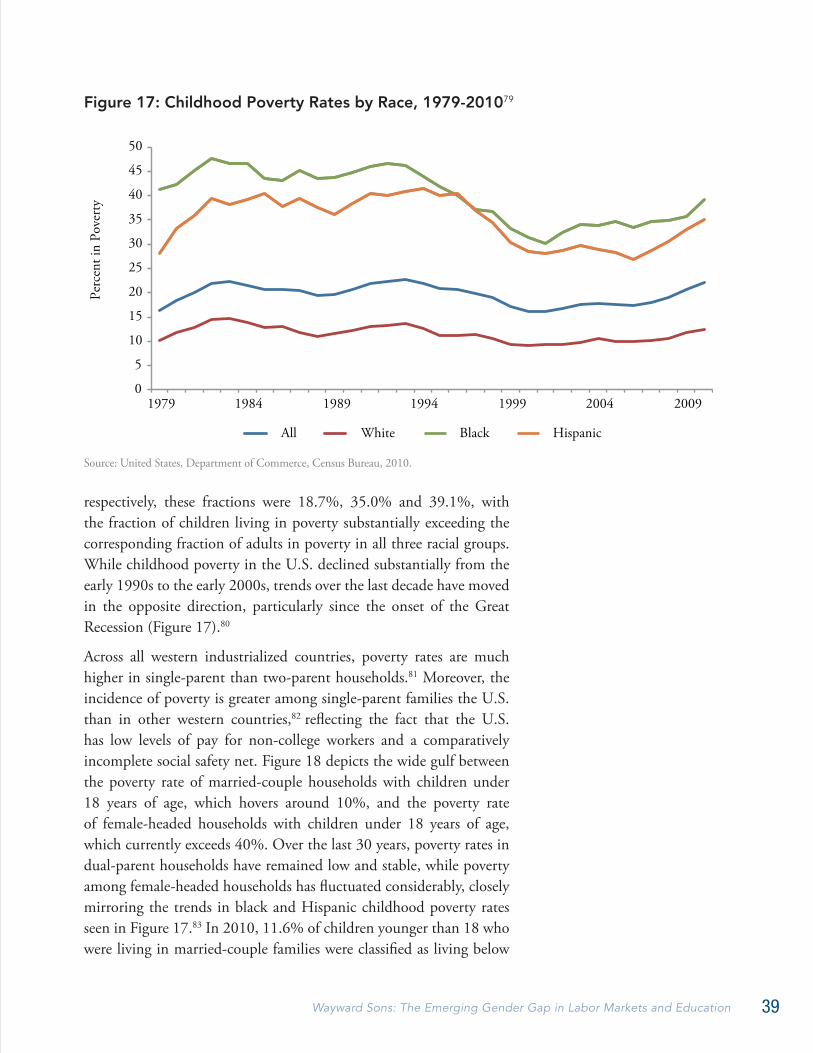
39Wayward Sons: The Emerging Gender Gap in Labor Markets and Education
respectively, these fractions were 18.7%, 35.0% and 39.1%, with the fraction of children living in poverty substantially exceeding the corresponding fraction of adults in poverty in all three racial groups. While childhood poverty in the U.S. declined substantially from the early 1990s to the early 2000s, trends over the last decade have moved in the opposite direction, particularly since the onset of the Great Recession (Figure 17).80
Across all western industrialized countries, poverty rates are much higher in single-parent than two-parent households.81 Moreover, the incidence of poverty is greater among single-parent families the U.S. than in other western countries,82 reflecting the fact that the U.S. has low levels of pay for non-college workers and a comparatively incomplete social safety net. Figure 18 depicts the wide gulf between the poverty rate of married-couple households with children under 18 years of age, which hovers around 10%, and the poverty rate of female-headed households with children under 18 years of age, which currently exceeds 40%. Over the last 30 years, poverty rates in dual-parent households have remained low and stable, while poverty among female-headed households has fluctuated considerably, closely mirroring the trends in black and Hispanic childhood poverty rates seen in Figure 17.83 In 2010, 11.6% of children younger than 18 who were living in married-couple families were classified as living below
0
5
10
15
20
25
30
35
40
45
50
1979 1984 1989 1994 1999 2004 2009
Perc
ent i
n Po
vert
y
All White Black Hispanic
Figure 17: Childhood Poverty Rates by Race, 1979-201079
Source: United States, Department of Commerce, Census Bureau, 2010.

40 T H I R D W AY N E X T
the poverty line, compared to a remarkable 46.9% of children living in single female-headed homes and 28.1% of children living in single male-headed homes. Thus, the rise in the number of single female-headed households in the U.S. implies that a substantial and rising fraction of U.S. children are potentially placed at a disadvantage from an early age.
Though there are numerous reasons to be concerned with childhood poverty, the most relevant for this paper is the robust relationship between household financial resources and the educational attainment of children. Consider for example Figure 19, reproduced from Bailey and Dynarski,85 which plots the relationship between family income, college-going, and college-completion for two cohorts of U.S. adults, those born in 1961 through 1964 (late Baby Boomers) and those born between 1979 and 1982 (early Millennials). Among Boomers, we see a steep positive relationship between household income and college attainment. Children born into the highest quartile of family incomes in 1961 through 1964 were 40 percentage points more likely to attend college and 30 percentage points more
0
10
20
30
40
50
60
1979 1984 1989 1994 1999 2004 2009
Perc
ent i
n Po
vert
y
All Married-Couple Male-householder, no wife present Female-householder, no husband present
Figure 18: Family Poverty Rates by Household Type, 1979-2010: Households with Children Under Age 1884
Source: United States, Department of Commerce, Census Bureau, 2010.
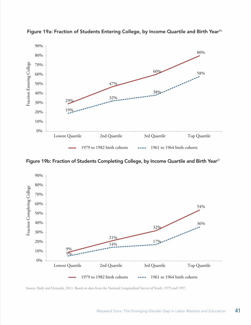
41Wayward Sons: The Emerging Gender Gap in Labor Markets and Education
29%
47%
60%
80%
19%
32% 38%
58%
0%
10%
20%
30%
40%
50%
60%
70%
80%
90%
Lowest Quartile 2nd Quartile 3rd Quartile Top Quartile
Frac
tion
Ente
ring
Col
lege
1979 to 1982 birth cohorts 1961 to 1964 birth cohorts
Figure 19a: Fraction of Students Entering College, by Income Quartile and Birth Year86
0%
10%
20%
30%
40%
50%
60%
70%
80%
90%
Lowest Quartile 2nd Quartile 3rd Quartile Top Quartile
Frac
tion
Com
plet
ing
Col
lege
1979 to 1982 birth cohorts 1961 to 1964 birth cohorts
9%
21%
32%
54%
5%
14% 17%
36%
Figure 19b: Fraction of Students Completing College, by Income Quartile and Birth Year87
Source: Baily and Dynarski, 2011. Based on data from the National Longitudinal Survey of Youth, 1979 and 1997.
42 T H I R D W AY N E X T
likely to complete college than children born into the lowest quartile of family incomes in the same years.
As highlighted by Figure 1 in the Introduction, the late Baby Boomer cohorts were at the low ebb of college-going relative to surrounding cohorts; college attendance and completion rose considerably in the intervening twenty years, particularly among women. One might have speculated that with the increasing rate of post-secondary education, household income might have become a less important determinant of college-going and college completion. In reality, Figure 19 reveals that the opposite occurred. Between the late Baby Boom and early Millennial generation, the gap in college-going between children of first and fourth quartile households rose sharply from 40 to 50 percentage points, while the gap in college-completions rose even more rapidly from 30 to 45 percentage points.
Although these disparities in college attainment between children of high and low-income families are not manifest until early adulthood, much evidence suggests that the underlying deficiencies in academic preparedness accrue much earlier. For example, recent work by Reardon88 finds that among cohorts born in the early 1960s, the gap in achievement on standardized readings tests between children raised in households at the 90th percentile versus 10th percentiles of the household income distribution was on the order of 0.85 standard deviations—comparable to the average black-white reading achievement gap in the same time period. Over the next four decades, this income-achievement gap widened by approximately an additional 40%, growing from 0.85 standard deviations among the 1960 cohorts to 1.20 standard deviations among the year 2000 birth cohort.89 These large and growing discrepancies in achievement between children of high and low-income households suggest that money matters—and, potentially, that it matters more than it used to.
It is natural to ask, however, whether the clear, positive relationship between family income and child achievement reflects a causal effect of family income on child achievement or merely a set of statistical associations that largely operate through other channels. Could it be the case, for example, that because higher income parents are also typically better-educated parents, the academic advantage of children of high income households stems primarily from parental education rather than parental income?
The effect of household resources per se on children’s outcomes is not a settled question in social science. Twenty years ago, the
These large and growing discrepancies in achievement between children of high and low-income households suggest that money matters—and, potentially, that it matters more than it used to.
43Wayward Sons: The Emerging Gender Gap in Labor Markets and Education
rough consensus view among economists was that the bulk of the relationship between income and achievement reflected factors other than the direct effect of income on children’s achievement.90 More recent evidence, however, has bolstered the view that family resources do play an important role in children’s outcomes. A paper by Dahl and Lochner,91 for example, analyzes changes in family income due to fluctuations in the generosity of the Earned Income Tax Credit. They find that a family income increase of $1000 raises children’s test scores in the short run by 6% of a standard deviation, with the largest effects found for boys, minority children, children of unmarried mothers, and children of less-educated mothers. Studying a set of welfare and antipoverty experiments conducted during the 1990s, a recent paper by Duncan, Morris, and Rodrigues92 finds effects of family income on children’s achievement of a similar magnitude to Dahl and Lochner. Given that the gaps in household incomes between poor and even middle-income families extend into the multiple tens of thousands of dollars, these results imply that differences in household resources may be a substantial contributor to the income-achievement gap. Though this research does not prove—or even suggest—that family income is the only important factor in determining children’s achievement, it establishes a strong case that money matters—material privation has a significant adverse causal effect on the skills development and ultimate educational attainment of U.S. children.93
Given the growing evidence that household resources affect children’s academic achievement—and particularly for children in disadvantaged households—the rising share of U.S. children reared in single-headed homes presents a prima facie cause for concern. The underlying concern is propagation of inequality. Education is the most effective mechanism available for promoting intergenerational economic mobility, and it is also one that enjoys widespread public support. The evidence above suggests that rising inequality of resources between children in affluent versus less-educated and minority households blunts this mechanism. This raises the concern that the current trajectory of inequality and the attendant changes in family structure will exacerbate the inequality of educational attainment and incomes in subsequent generations.
Inequality of Parental Resources
We finally turn our attention to the potentially profound implications of changing family structure with particularly adverse implications for boys: a diminished role for adult men in their biological children’s
The underlying concern is propagation of inequality.
44 T H I R D W AY N E X T
lives. We noted above that the shift in household structures among less-educated and minority adults towards resource-poor, female-headed households may propagate the intergenerational transmission of inequality. For boys, there is a further consequence: the diminished involvement of the related male parent may magnify the emerging gender gap in educational attainment and labor market outcomes. Although male and female children within a given household are theoretically exposed to the same environment—including schools, neighborhoods, and adult guardians—the increasing prevalence of female-headed households implies that the majority of girls continue to cohabit with their same-sex biological parent who will likely serve as a same-sex role model. By contrast, male children raised in female-headed households are less likely to have a positive male adult household member present that serves an analogous role. A growing body of evidence, summarized below, indicates that the absence of stable fathers from children’s lives has particularly significant adverse consequences for boys’ psychosocial development and educational achievement.
While it would be inaccurate to claim that social science has reached consensus on the differential effects that parents have on the social and educational development of their same-sex children, recent data suggest that the female advantage in educational attainment is substantially more pronounced in female-headed households and in households where the father is less educated than the mother. For example, comparing the educational attainments of children born in the late 1960s according to both the educational attainment of their parents and the presence of the father in the household, Buchman and DiPrete94 document a large female advantage in college completion—on the order of 10 to 14 percentage points—in households where the mother has at least some college education and the father is either less educated than the mother or is absent. By contrast, in households where the father is both present and highly educated (some college or above), boys and girls are about equally likely to complete college. Additionally, children of both sexes are substantially more likely to complete college when the mother and father both have some college education. Evidence from a study by Brian Jacob95 corroborates this regularity: after controlling for a host of individual and family characteristics, growing up in a single-parent home appears to significantly decrease the probability of college attendance for boys, yet has no similar effect for girls.96 Putting these pieces together, we tentatively conclude that boys perform less well academically than girls
...the diminished involvement of the related male parent may magnify the emerging gender gap in educational attainment and labor market outcomes.
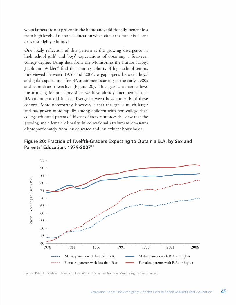
45Wayward Sons: The Emerging Gender Gap in Labor Markets and Education
when fathers are not present in the home and, additionally, benefit less from high levels of maternal education when either the father is absent or is not highly educated.
One likely reflection of this pattern is the growing divergence in high school girls’ and boys’ expectations of obtaining a four-year college degree. Using data from the Monitoring the Future survey, Jacob and Wilder97 find that among cohorts of high school seniors interviewed between 1976 and 2006, a gap opens between boys’ and girls’ expectations for BA attainment starting in the early 1980s and cumulates thereafter (Figure 20). This gap is at some level unsurprising for our story since we have already documented that BA attainment did in fact diverge between boys and girls of these cohorts. More noteworthy, however, is that the gap is much larger and has grown more rapidly among children with non-college than college-educated parents. This set of facts reinforces the view that the growing male-female disparity in educational attainment emanates disproportionately from less educated and less affluent households.
40
45
50
55
60
65
70
75
80
85
90
95
1976 1981 1986 1991 1996 2001 2006
Perc
ent E
xpec
ting
to E
arn
a B.
A.
Males, parents with less than B.A. Males, parents with B.A. or higher
Females, parents with less than B.A. Females, parents with B.A. or higher
Figure 20: Fraction of Twelfth-Graders Expecting to Obtain a B.A. by Sex and Parents’ Education, 1979-200798
Source: Brian L. Jacob and Tamara Linkow Wilder, Using data from the Monitoring the Future survey.
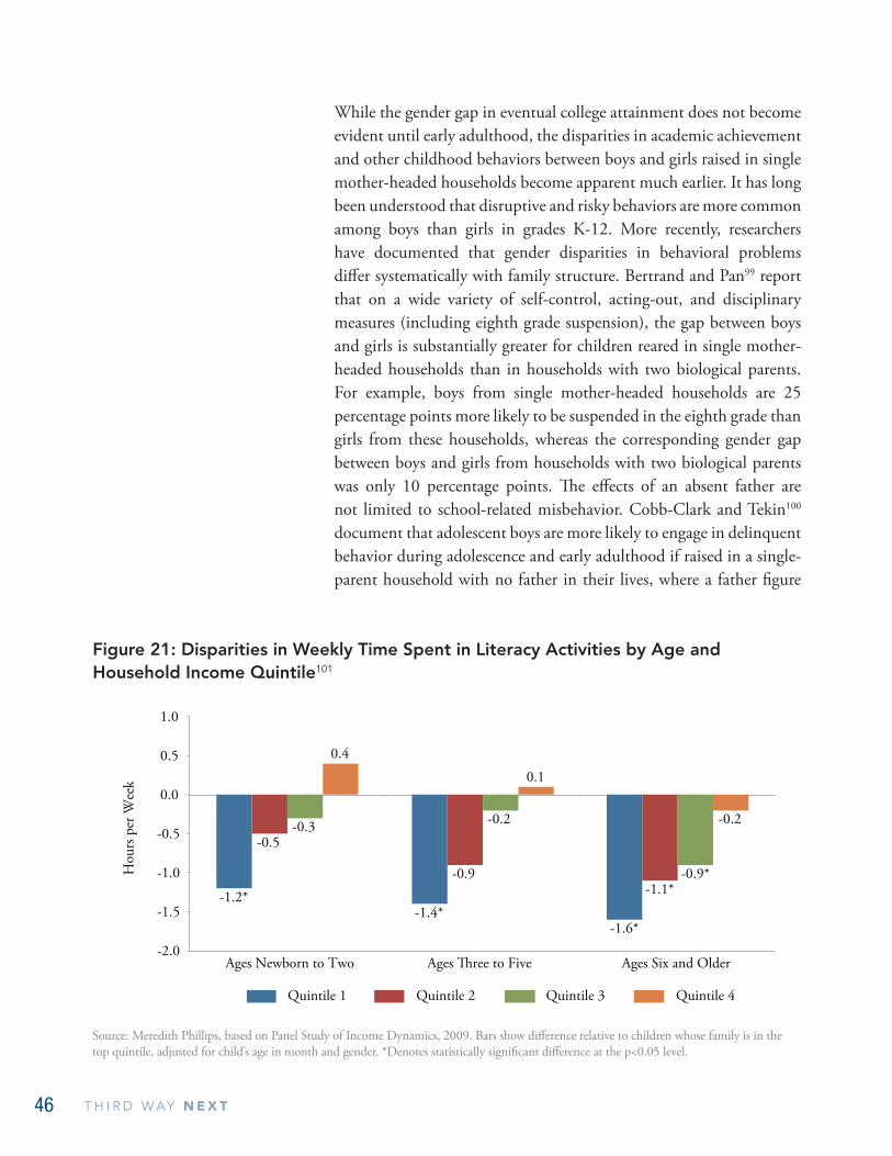
46 T H I R D W AY N E X T
While the gender gap in eventual college attainment does not become evident until early adulthood, the disparities in academic achievement and other childhood behaviors between boys and girls raised in single mother-headed households become apparent much earlier. It has long been understood that disruptive and risky behaviors are more common among boys than girls in grades K-12. More recently, researchers have documented that gender disparities in behavioral problems differ systematically with family structure. Bertrand and Pan99 report that on a wide variety of self-control, acting-out, and disciplinary measures (including eighth grade suspension), the gap between boys and girls is substantially greater for children reared in single mother-headed households than in households with two biological parents. For example, boys from single mother-headed households are 25 percentage points more likely to be suspended in the eighth grade than girls from these households, whereas the corresponding gender gap between boys and girls from households with two biological parents was only 10 percentage points. The effects of an absent father are not limited to school-related misbehavior. Cobb-Clark and Tekin100 document that adolescent boys are more likely to engage in delinquent behavior during adolescence and early adulthood if raised in a single-parent household with no father in their lives, where a father figure
-1.2* -1.4*
-1.6*
-0.5
-0.9 -1.1*
-0.3 -0.2
-0.9*
0.4
0.1
-0.2
-2.0
-1.5
-1.0
-0.5
0.0
0.5
1.0
Ages Newborn to Two Ages �ree to Five Ages Six and Older
Hou
rs p
er W
eek
Quintile 1 Quintile 2 Quintile 3 Quintile 4
Figure 21: Disparities in Weekly Time Spent in Literacy Activities by Age and Household Income Quintile101
Source: Meredith Phillips, based on Panel Study of Income Dynamics, 2009. Bars show difference relative to children whose family is in the top quintile, adjusted for child’s age in month and gender. *Denotes statistically significant difference at the p<0.05 level.
47Wayward Sons: The Emerging Gender Gap in Labor Markets and Education
category includes both biological (residential or nonresidential) and step-fathers.102
Why might living in a single mother-headed household exacerbate existing gender differences in behavioral problems? One potential channel is parental time use, with single parents presumably more limited in the amount of time they can devote to childcare activities. For example, Figure 21, sourced from a study by Meredith Phillips,103 documents substantial differences by household income level in the amount of time that parents devote weekly to literacy activities (primarily reading) with their children at all age levels. Children reared in the top quintile of the family income distribution are read to by their parents approximately 1.2 hours more per week than children from households in the bottom quintile.104 In fact, over the last twenty years, there has been a tremendous increase in the hours per week that more highly educated parents devote to childcare activities, with a much more moderate rise in the amount of time for less educated parents.105 If boys are more responsive to parental inputs (or the absence thereof ) than are girls, then it is possible that the gender gradient in behavioral and academic development could be magnified in single-parent households.106 In addition to the disparities in the amount and type of parental interaction by household type, single mothers also appear to interact differently with their sons and daughters. Bertrand and Pan107 find that single mothers spend an hour less per week with their sons than with their daughters, report feeling more emotionally distant from their sons, and engage in disciplinary action such as spanking more frequently with their sons. These disparities in parenting are largely absent from dual parent homes.
A complementary channel by which family structure may affect children’s outcomes and aspirations is through role modeling. If children aim to emulate the adult roles of their same-sex parent, then girls may increasingly expect to fully support both themselves and their children whereas, conversely, males may come to anticipate a less central or more transient role. Currently, in all but the highest socioeconomic quintile, females far outpace males in their expectations of obtaining college and graduate degrees.108 From 1990 until 2000, the gap in the percentage of tenth grade males and females who expected to obtain at least a bachelor’s degree widened substantially among the lowest three income quintiles.109 Female expectations of future labor force participation have also rapidly increased over the last thirty years.110 These patterns are broadly
If children aim to emulate the adult roles of their same-sex parent, then girls may increasingly expect to fully support both themselves and their children whereas, conversely, males may come to anticipate a less central or more transient role.
48 T H I R D W AY N E X T
consistent with the hypothesis that changes in household structure have fomented a gender divergence in educational expectations, but the evidence is far from definitive at present.
A central difficulty in distinguishing the direct effects of male parental absence per se on children’s psychosocial development apart from the effects of lower income levels, less advantageous school and neighborhood environments, reduced parental time availability, and higher household stress levels is that children raised in single mother-headed households are likely to be exposed to all of these potential risk factors. Accordingly, male parental absence may appear to differentially disadvantage boys because boys are more sensitive than girls to either male role models or to these other factors.
Perhaps the best available evidence that potentially distinguishes these two channels comes from an ambitious, large-scale randomized social experiment, the Moving to Opportunity (MTO) program that was initiated in the early 1990s. MTO was designed to improve the well-being of adults and children living in high poverty public housing by enabling them to move into outlying communities where poverty rates were substantially lower. One of the most surprising (and firmly established) set of results from the large body of research produced by the MTO experiment is that moving families to low-poverty neighborhoods outside of the central city had starkly different effects on boys and girls. Girls in treated households obtained better academic outcomes, engaged in fewer risky behaviors, and reported better physical health than girls in control households (that is, those who remained in public housing projects or received standard “Section 8” housing vouchers). By contrast, boys in treated households fared substantially worse on these same outcomes than did boys in control households,111 including experiencing higher rates of arrest, poorer health, and greater abuse of drugs and alcohols.
Because household participation in the MTO treatment versus control groups was randomly assigned, differences in household incomes or parental time availability between treatment and control households are unlikely to be the explanation for why girls benefited from the treatment while boys did not. Similarly, the quality of schools that children attended, the safety of the neighborhoods in which they resided, and even the mental health of the mothers who headed these households were all positively affected by the experiment—again suggesting that these factors are not likely to be the root of the gender disparity in treatment effects.
...moving families to low-poverty neighborhoods outside of the central city had starkly different effects on boys and girls.
49Wayward Sons: The Emerging Gender Gap in Labor Markets and Education
Almost by a process of elimination, researchers have recognized that one of the most cogent explanation for why boys in the treatment group fared worse than those in the control group is the effect that the experiment had on reducing the presence of male role models. Because essentially all MTO households were female-headed, and because the low-poverty neighborhoods into which families moved were typically not nearby to the inner-city locations where they previously resided, the MTO experiment reduced subsequent interactions between experimental household members and their friends and relatives from their prior neighborhoods. As Clampet-Lundquist, Kling, Edin, and Duncan112 observe, the MTO experiment significantly reduced the role of fathers and father-figures in children’s lives among households in the treatment group, which may in part explain the adverse impact of the experiment on boys.
We must stress, however, that this explanation should be taken as tentative and potentially incomplete. Clampet-Lundquist et al. also emphasize that boys belonging to MTO treatment households developed less successful mechanisms for fitting in with neighborhood norms, for interacting with peers, and for navigating risky neighborhood situations (including violence associated with drug-trafficking) than did boys in control households.113 One may speculate that these symptoms of maladjustment among boys in the treatment group could also be explained by the reduced presence of male role models in their lives. Alternatively, these adverse outcomes may reflect the particular difficulties that black inner-city youth face when moving into suburban neighborhoods.
While more research will be needed to gain a fuller understanding of the stark gender differences that emerged in developmental and educational outcomes in the course of the MTO experiment, one hypothesis that the MTO results do appear to support is this: boys in single female-headed families are particularly at risk for adverse outcomes across many domains, including high school dropout, criminality, and violence. This reinforces our view that the emerging gender gap in educational and labor market outcomes is explained in part by changes in U.S. household structures, which are themselves fomented by the declining labor market opportunities faced by non-college males. These developments appear to have inadvertently placed boys at particular risk for reduced academic achievement and diminished chances of obtaining stable employment with earnings levels sufficient to support a family.
...boys in single female-headed families are particularly at risk for adverse outcomes across many domains, including high school dropout, criminality, and violence.
50 T H I R D W AY N E X T
CONCLUSION The emerging gender gaps in educational attainment and labor market advancement will pose two considerable challenges for social and economic policy. First, due to the rising importance of education over the last three decades as a determinant of lifetime income—and, more concretely, due to the sharply deteriorating earnings and employment prospects of less-educated U.S. workers—the stagnation of male educational attainment bodes ill for the well-being of recent cohorts of U.S. males, particularly minorities and those from low-income households. Less-educated males of recent cohorts are likely to face diminished employment and earnings opportunities and other attendant maladies, including poorer health, higher probability of incarceration, and generally lower life satisfaction.
A second challenge posed by these developments is the impact that stagnating male educational attainment and diminished male labor market opportunities are likely to have on the well-being of children and potential mates. Due to lower marriage rates of less-educated males, their children face comparatively low odds of living in economically secure households with two parents present. Unsurprisingly, children born into such households also face poorer educational and earnings prospects over the long term. Even more concerning is that male children born into low-income, single-parent headed households—which, in the vast majority of cases are female-headed households—appear to fare particularly poorly on numerous social and educational outcomes. A vicious cycle may ensue, with the poor economic prospects of less-educated males creating differentially large disadvantages for their sons, thus potentially reinforcing the development of the gender gap in the next generation.
Sorting out the causal factors behind these trends is a challenging but nonetheless central topic for social science research and public policy. A growing body of evidence supports the hypothesis that the erosion of labor market opportunities for low-skill workers in general—and non-college males in particular—has catalyzed a fall in employment and earnings among less-educated males and a decline in the marriage rates of less-educated males and females. These developments in turn diminish family stability, reduce household financial resources, and subtract from the stock of parental time and attention that should play a critical role in fomenting the educational achievement and economic advancement of the next generation.
51Wayward Sons: The Emerging Gender Gap in Labor Markets and Education
The topic is sufficiently important in our view—and the trends sufficiently stark—that it is not premature to engage in productive discussion, even if the clarity of our knowledge is well short of the urgency of the subject. It also should be clear that while this paper focuses on the cloudy future of boys, we celebrate the progress of girls. As our discussion above highlights, the well-being of both sexes is linked through, among other factors, family formation, child-rearing, and economic interdependency.
As the importance of educational investments for earnings has magnified, differences in educational attainment and family formation among socioeconomic, racial, and gender groups have become an increasingly important differentiator in the life chances of children. Developing mechanisms to foment educational opportunity and economic mobility, and to mitigate the role of initial birth disparities in shaping the life course of current and future generations of young Americans, is an increasingly critical agenda item for social policy.
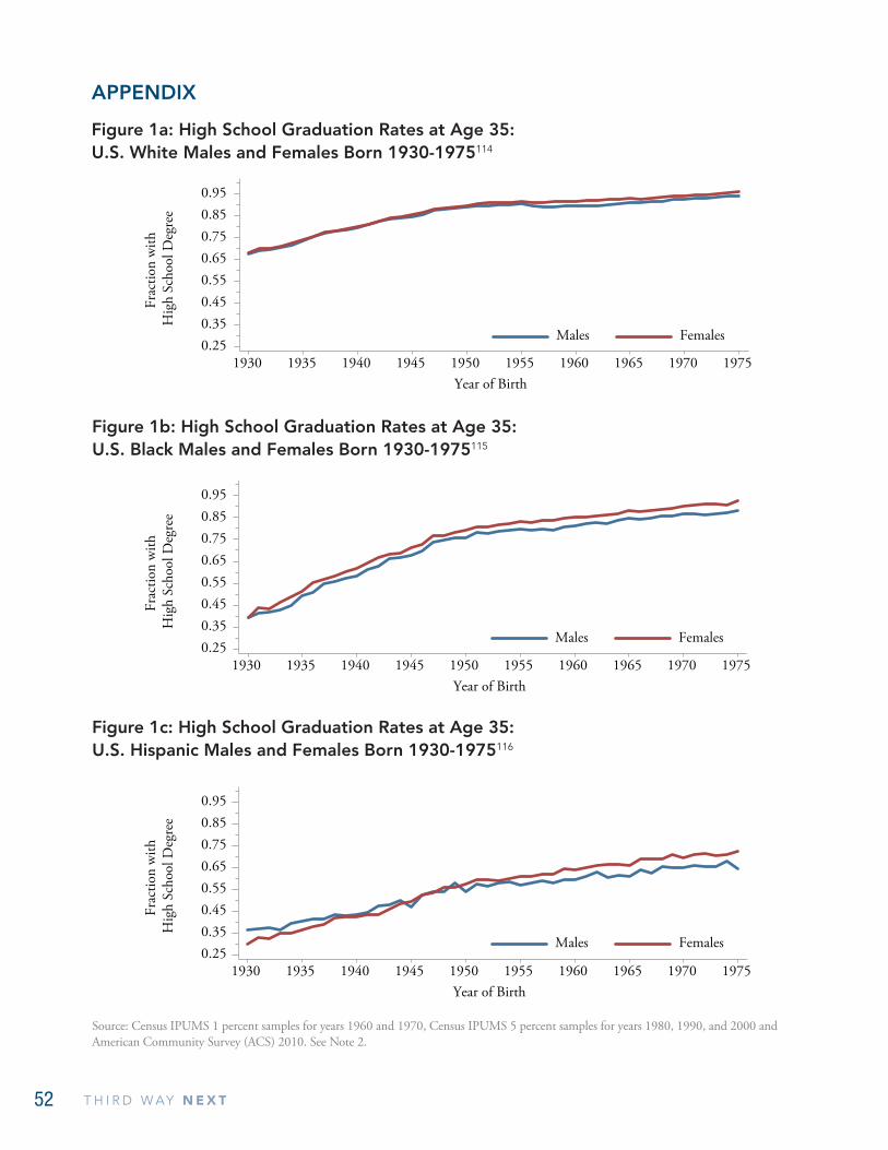
52 T H I R D W AY N E X T
0.250.350.450.550.650.750.850.95
Frac
tion
with
H
igh
Scho
ol D
egre
e
1930 1935 1940 1945 1950 1955 1960 1965 1970 1975Year of Birth
Males Females
1930 1935 1940 1945 1950 1955 1960 1965 1970 1975Year of Birth
Males Females0.250.350.450.550.650.750.850.95
1930 1935 1940 1945 1950 1955 1960 1965 1970 1975Year of Birth
Males Females0.250.350.450.550.650.750.850.95
Frac
tion
with
H
igh
Scho
ol D
egre
eFr
actio
n w
ith
Hig
h Sc
hool
Deg
ree
APPENDIX
Figure 1a: High School Graduation Rates at Age 35: U.S. White Males and Females Born 1930-1975114
Figure 1b: High School Graduation Rates at Age 35: U.S. Black Males and Females Born 1930-1975115
Figure 1c: High School Graduation Rates at Age 35: U.S. Hispanic Males and Females Born 1930-1975116
Source: Census IPUMS 1 percent samples for years 1960 and 1970, Census IPUMS 5 percent samples for years 1980, 1990, and 2000 and American Community Survey (ACS) 2010. See Note 2.
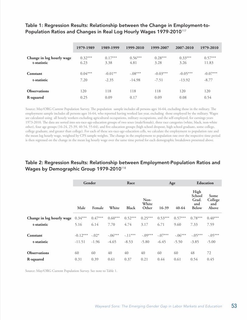
53Wayward Sons: The Emerging Gender Gap in Labor Markets and Education
Table 1: Regression Results: Relationship between the Change in Employment-to-Population Ratios and Changes in Real Log Hourly Wages 1979-2010117
Source: May/ORG Current Population Survey. The population sample includes all persons ages 16-64, excluding those in the military. The employment sample includes all persons ages 16-64, who reported having worked last year, excluding those employed by the military. Wages are calculated using all hourly workers excluding agricultural occupations, military occupations, and the self-employed, for earnings years 1973-2010. The data are sorted into sex-race-age-education groups of two sexes (male/female), three race categories (white, black, non-white other), four age groups (16-24, 25-39, 40-54, 55-64), and five education groups (high school dropout, high school graduate, some college, college graduate, and greater than college). For each of these sex-race-age-education cells, we calculate the employment to population rate and the mean log hourly wage, weighted by CPS sample weights. The change in the employment to population rate over the respective time period is then regressed on the change in the mean log hourly wage over the same time period for each demographic breakdown presented above.
1979-1989 1989-1999 1999-2010 1999-2007 2007-2010 1979-2010
Change in log hourly wage 0.32*** 0.17*** 0.56*** 0.28*** 0.33*** 0.57***t-statistic 6.23 3.38 4.81 3.28 3.26 11.83
Constant 0.04*** -0.01** -.08*** -0.03*** -0.05*** -0.07***t-statistic 7.20 -2.35 -14.98 -7.51 -13.92 -8.77
Observations 120 118 118 118 120 120R-squared 0.25 0.09 0.17 0.09 0.08 0.54
Table 2: Regression Results: Relationship between Employment-Population Ratios and Wages by Demographic Group 1979-2010118
Source: May/ORG Current Population Survey. See note to Table 1.
Gender Race Age Education
Male Female White Black
Non-White Other 16-39 40-64
High School Grad. and
Below
Some College
and Above
Change in log hourly wage 0.34*** 0.47*** 0.60*** 0.52*** 0.25*** 0.53*** 0.57*** 0.78*** 0.40***t-statistic 5.16 6.14 7.70 4.74 3.17 6.71 9.60 7.33 7.59
Constant -0.12*** -.02* -.06*** -.11*** -.09*** -.07*** -.06*** -.05*** -.05***t-statistic -11.51 -1.96 -4.65 -8.53 -5.80 -6.45 -5.50 -3.85 -5.00
Observations 60 60 40 40 40 60 60 48 72R-squared 0.31 0.39 0.61 0.37 0.21 0.44 0.61 0.54 0.45
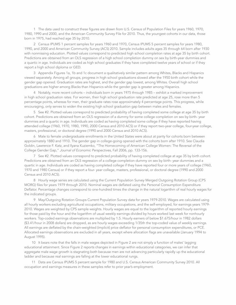
1 The data used to construct these figures are drawn from U.S. Census of Population Files for years 1960, 1970, 1980, 1990 and 2000, and the American Community Survey File for 2010. Thus, the youngest cohorts in our data, those born in 1975, had reached age 35 by 2010.
2 Census IPUMS 1 percent samples for years 1960 and 1970, Census IPUMS 5 percent samples for years 1980, 1990, and 2000 and American Community Survey (ACS) 2010. Sample includes adults ages 35 through 64 born after 1930 with nonmissing education. Plotted values correspond to predicted high school completion rates at age 35 by birth cohort. Predictions are obtained from an OLS regression of a high school completion dummy on sex by birth-year dummies and a quartic in age. Individuals are coded as high school graduates if they have completed twelve years of school or if they report a high school diploma or GED.
3 Appendix Figures 1a, 1b and 1c document a qualitatively similar pattern among Whites, Blacks and Hispanics viewed separately. Among all groups, progress in high school graduations slowed after the 1950 birth cohort while the gender gap opened. Graduation rates are highest, and the gender gap lowest, among Whites. Overall high school graduations are higher among Blacks than Hispanics while the gender gap is greater among Hispanics.
4 Notably, more recent cohorts – individuals born in years 1975 through 1985 – exhibit a marked improvement in high school graduation rates. For women, their high school graduation rate predicted at age 25, rose more than 5 percentage points, whereas for men, their graduate rates rose approximately 4 percentage points. This progress, while encouraging, only serves to widen the existing high school graduation gap between males and females.
5 See #2. Plotted values correspond to predicted probability of having completed some college at age 35 by birth cohort. Predictions are obtained from an OLS regression of a dummy for some college completion on sex by birth- year dummies and a quartic in age. Individuals are coded as having completed some college if they have reported having attended college (1960, 1970, 1980, 1990, 2000 Census and 2010 ACS) or if they report two-year college, four-year college, masters, professional, or doctoral degree (1990 and 2000 Census and 2010 ACS).
6 Male to female undergraduate enrollments in the United States were about at parity for cohorts born between approximately 1880 and 1910. The gender gap in college-going opened with the cohorts born after 1910. See Claudia Goldin, Lawrence F. Katz, and Ilyana Kuziemko, “The Homecoming of American College Women: The Reversal of the College Gender Gap,” Journal of Economic Perspectives, Fall 2006, pp. 133-156.
7 See #2. Plotted values correspond to predicted probability of having completed college at age 35 by birth cohort. Predictions are obtained from an OLS regression of a college completion dummy on sex by birth- year dummies and a quartic in age. Individuals are coded as having completed college if they have reported four or more years of college (1960, 1970 and 1980 Census) or if they report a four- year college, masters, professional, or doctoral degree (1990 and 2000 Census and 2010 ACS).
8 Hourly wage series are calculated using the Current Population Survey Merged Outgoing Rotation Group (CPS MORG) files for years 1979 through 2010. Nominal wages are deflated using the Personal Consumption Expenditure Deflator. Percentage changes correspond to one-hundred times the change in the natural logarithm of real hourly wages for the indicated groups.
9 May/Outgoing Rotation Groups Current Population Survey data for years 1979-2010. Wages are calculated using all hourly workers excluding agricultural occupations, military occupations, and the self-employed, for earnings years 1979-2010. Wages are weighted by CPS sample weights. Hourly wages are equal to the logarithm of reported hourly earnings for those paid by the hour and the logarithm of usual weekly earnings divided by hours worked last week for nonhourly workers. Top-coded earnings observations are multiplied by 1.5. Hourly earners of below $1.675/hour in 1982 dollars ($3.41/hour in 2008 dollars) are dropped, as are hourly wages exceeding 1/35th the top-coded value of weekly earnings. All earnings are deflated by the chain-weighted (implicit) price deflator for personal consumption expenditures, or PCE. Allocated earnings observations are excluded in all years, except where allocation flags are unavailable (January 1994 to August 1995).
10 It bears note that the falls in male wages depicted in Figure 2 are not simply a function of males’ lagging educational attainment. Since Figure 2 reports changes in earnings within educational categories, we can infer that aggregate male wage growth is stagnating both because men are not advancing particularly rapidly up the educational ladder and because real earnings are falling at the lower educational rungs.
11 Data are Census IPUMS 5 percent sample for 1980 and U.S. Census American Community Survey 2010. All occupation and earnings measures in these samples refer to prior year’s employment.
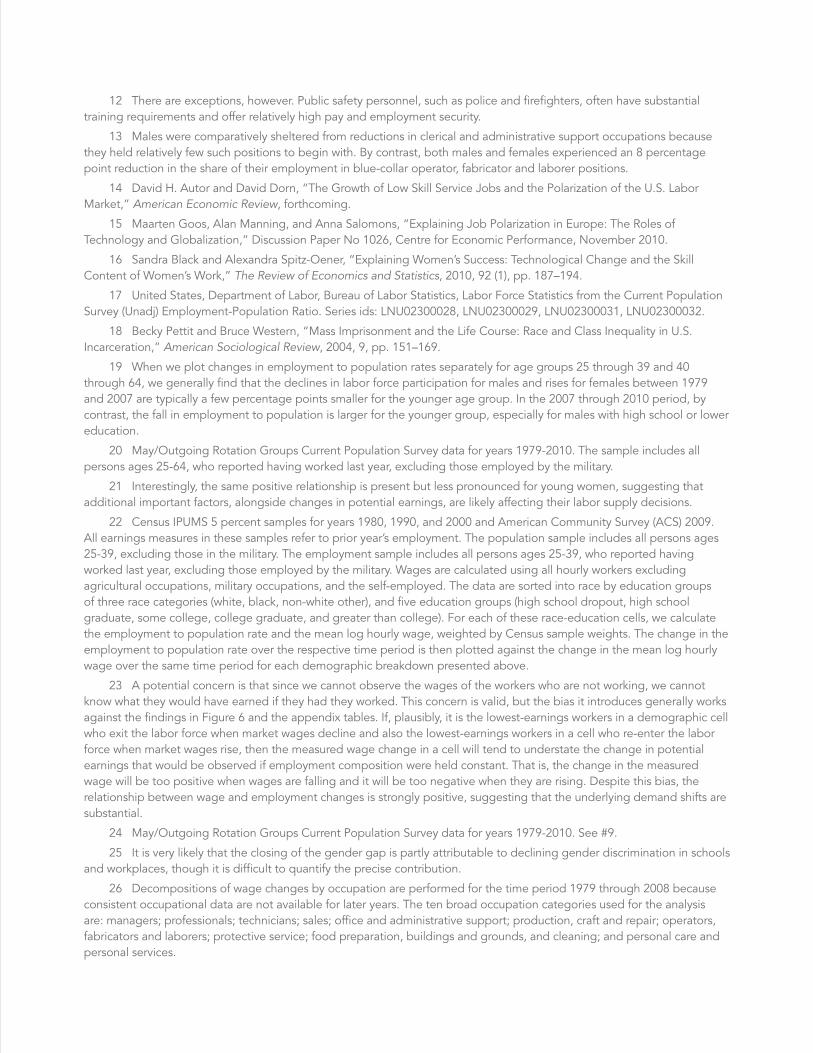
12 There are exceptions, however. Public safety personnel, such as police and firefighters, often have substantial training requirements and offer relatively high pay and employment security.
13 Males were comparatively sheltered from reductions in clerical and administrative support occupations because they held relatively few such positions to begin with. By contrast, both males and females experienced an 8 percentage point reduction in the share of their employment in blue-collar operator, fabricator and laborer positions.
14 David H. Autor and David Dorn, “The Growth of Low Skill Service Jobs and the Polarization of the U.S. Labor Market,” American Economic Review, forthcoming.
15 Maarten Goos, Alan Manning, and Anna Salomons, “Explaining Job Polarization in Europe: The Roles of Technology and Globalization,” Discussion Paper No 1026, Centre for Economic Performance, November 2010.
16 Sandra Black and Alexandra Spitz-Oener, “Explaining Women’s Success: Technological Change and the Skill Content of Women’s Work,” The Review of Economics and Statistics, 2010, 92 (1), pp. 187–194.
17 United States, Department of Labor, Bureau of Labor Statistics, Labor Force Statistics from the Current Population Survey (Unadj) Employment-Population Ratio. Series ids: LNU02300028, LNU02300029, LNU02300031, LNU02300032.
18 Becky Pettit and Bruce Western, “Mass Imprisonment and the Life Course: Race and Class Inequality in U.S. Incarceration,” American Sociological Review, 2004, 9, pp. 151–169.
19 When we plot changes in employment to population rates separately for age groups 25 through 39 and 40 through 64, we generally find that the declines in labor force participation for males and rises for females between 1979 and 2007 are typically a few percentage points smaller for the younger age group. In the 2007 through 2010 period, by contrast, the fall in employment to population is larger for the younger group, especially for males with high school or lower education.
20 May/Outgoing Rotation Groups Current Population Survey data for years 1979-2010. The sample includes all persons ages 25-64, who reported having worked last year, excluding those employed by the military.
21 Interestingly, the same positive relationship is present but less pronounced for young women, suggesting that additional important factors, alongside changes in potential earnings, are likely affecting their labor supply decisions.
22 Census IPUMS 5 percent samples for years 1980, 1990, and 2000 and American Community Survey (ACS) 2009. All earnings measures in these samples refer to prior year’s employment. The population sample includes all persons ages 25-39, excluding those in the military. The employment sample includes all persons ages 25-39, who reported having worked last year, excluding those employed by the military. Wages are calculated using all hourly workers excluding agricultural occupations, military occupations, and the self-employed. The data are sorted into race by education groups of three race categories (white, black, non-white other), and five education groups (high school dropout, high school graduate, some college, college graduate, and greater than college). For each of these race-education cells, we calculate the employment to population rate and the mean log hourly wage, weighted by Census sample weights. The change in the employment to population rate over the respective time period is then plotted against the change in the mean log hourly wage over the same time period for each demographic breakdown presented above.
23 A potential concern is that since we cannot observe the wages of the workers who are not working, we cannot know what they would have earned if they had they worked. This concern is valid, but the bias it introduces generally works against the findings in Figure 6 and the appendix tables. If, plausibly, it is the lowest-earnings workers in a demographic cell who exit the labor force when market wages decline and also the lowest-earnings workers in a cell who re-enter the labor force when market wages rise, then the measured wage change in a cell will tend to understate the change in potential earnings that would be observed if employment composition were held constant. That is, the change in the measured wage will be too positive when wages are falling and it will be too negative when they are rising. Despite this bias, the relationship between wage and employment changes is strongly positive, suggesting that the underlying demand shifts are substantial.
24 May/Outgoing Rotation Groups Current Population Survey data for years 1979-2010. See #9.
25 It is very likely that the closing of the gender gap is partly attributable to declining gender discrimination in schools and workplaces, though it is difficult to quantify the precise contribution.
26 Decompositions of wage changes by occupation are performed for the time period 1979 through 2008 because consistent occupational data are not available for later years. The ten broad occupation categories used for the analysis are: managers; professionals; technicians; sales; office and administrative support; production, craft and repair; operators, fabricators and laborers; protective service; food preparation, buildings and grounds, and cleaning; and personal care and personal services.
27 It is of course possible that a more detailed breakdown of employment into narrow industry and occupation categories would indicate that a larger share of the observed female-male wage convergence is explained by gender differences in employment across categories with rising versus falling wages rather than by gender differences in wage changes within categories. It is nevertheless remarkable that almost none of the wage convergence seen here can be explained by the pronounced gender differences in occupational employment by education within the ten broad categories used for this exercise.
28 David H. Autor, Frank Levy, and Richard J. Murnane, “The Skill Content of Recent Technological Change: An Empirical Exploration,” The Quarterly Journal of Economics, 2003, 118 (4), pp. 1279–1333; See also Claudia Goldin and Lawrence F. Katz, The Race Between Education and Technology, Belknap Press, 2008.
29 Barry T. Hirsch, “Sluggish Institutions in a Dynamic World: Can Unions and Industrial Competition Coexist?” Journal of Economic Perspectives, March 2008, 22 (1), pp. 153–176. Updated data to 2011 online at www.unionstats.com. High rates of union penetration in the public sector, averaging over 35%, in part mask the private sector union decline when public and private sector unionization rates are combined. In 2011, the aggregate union membership rate (averaging over public and private sector workers) was 11.4%, which is nearly twice the private sector rate of 6.9%.
30 Sergio Firpo, Nicole M. Fortin, and Thomas Lemieux, “Occupational Tasks and Changes in the Wage Structure,” 2011; See also John E. DiNardo, Nicole M. Fortin, and Thomas Lemieux, “Labor Market Institutions and the Distribution of Wages, 1973-1992: A Semiparametric Approach,” Econometrica, 1996, 64 (5), pp. 1001–1044; See also Brigham R. Frandsen, “Why Unions Still Matter : The Effects of Unionization on the Distribution of Employee Earnings” 2012, pp.1–45; See also David Card, Thomas Lemieux, and W. Craig Riddell, “Unions and Wage Inequality,” in James T. Bennett and Bruce E. Kaufman, eds., What Do Unions Do? A Twenty-Year Perspective, New Brunswick, NJ: Transaction Publishers, 2007, pp. 114–159. Most studies of the impact of deunionization on wage structure focus on impacts on wage inequality—that is, the dispersion of wages—rather than real wage levels. While we loosely equate the two in the text above, there is even less certainty about the effect of deunionization on wage levels than on wage inequality.
31 David H. Autor, David Dorn, and Gordon H. Hanson, “The China Syndrome: Local Labor Market Effects of Import Competition in the United States,” American Economic Review, forthcoming.
32 Christian Broda and David E. Weinstein, “Globalization and the Gains from Variety,” Quarterly Journal of Economics, 2006, 121 (2), pp. 541–585.
33 Autor, Dorn and Hanson, forthcoming.
34 Daron Acemoglu, Philippe Aghion, and Giovanni L. Violante, “Deunionization, Technical Change and Inequality,” Carnegie-Rochester Conference, 2001, 55, pp. 229–264.
35 Paul Beaudry and Ethan Lewis, “Do Male-female Wage Differentials Reflect Differences in the Return to Skill?” NBER Working Paper 18159, 2012; See also Black and Spitz-Oener, 2010; See also Casey B. Mulligan and Yona Rubinstein, “Selection, investment, and women’s relative wages over time,” Quarterly Journal of Economics, August 2008; See also Finis Welch, “Growth in Womens Relative Wages and Inequality Among Men: One Phenomenon or Two?” American Economic Review, 2000, 90 (2), pp. 444–449.
36 Casey B. Mulligan and Yona Rubinstein, “Selection, investment, and women’s relative wages over time,” Quarterly Journal of Economics, August 2008.
37 In addition to the hypotheses discussed above, two other factors may explain in part why wage trends for non-college females have been more favorable than among similarly educated males: one is that non-college women have effectively ‘swam upstream’ against falling demand for non-college workers by improving their skills and workplace experience (See Francine D. Blau and Lawrence M. Kahn, “Swimming Upstream: Trends in the Gender Wage Differential in the 1980s” Journal of Labor Economics , Vol. 15(1), January 1997, pp. 1-42; a second possibility is that the prevalence of employer discrimination against women has fallen even as demand for less-educated labor has eroded. Either or both forces may contribute to an explanation for why wages of non-college females have risen modestly even as wages of similarly-educated males have declined sharply.
38 May/Outgoing Rotation Groups Current Population Survey data for years 1979-2010. See #9.
39 If we instead focus on older workers ages 40-64, the initial difference in the college/high-school earnings gap is closely comparable between males and females, while the growth in this differential is substantial for both sexes, smaller than among younger workers, and slightly greater among older females than older males. We highlight the patterns among younger workers in Figure 7 since these earnings differentials should be most relevant to young adults when considering their educational investments.
40 Claudia Goldin and Lawrence F. Katz, The Race between Education and Technology, Belknap Press, 2008.
41 Christopher Avery and Sarah Turner, “Student Loans: Do College Students Borrow Too Much, Or Not Enough?” Journal of Econonmic Perspectives, 2012, 26 (1), pp. 165–192.
42 Popular press accounts often portray a so-called college debt bubble wherein young adults emerge from their baccalaureate studies with crushing debt and poor job prospects. These stories are deeply misleading. With the U.S. labor market enduring its longest employment slump since the Great Depression, it is no surprise that almost all recent labor market entrants are doing badly. But both prior to and during the Great Recession, young college graduates have had substantially lower unemployment rates and substantially higher earnings than non-college grads. As the labor market improves in the years ahead, the chasm in earnings and opportunity between young adults who have completed college and those who have not will only grow wider.
43 May/Outgoing Rotation Groups Current Population Survey data for years 1979-2010. See #9.
44 Notably, the male earnings advantage at each education level among younger workers is substantially smaller in relative and absolute terms than among older workers, underscoring the fact that these gender differentials are eroding. Also surprising is that the proportional male earnings advantage among young adults is lowest among the most educated and highest among the least educated. For example, males ages 25-39 with a post-college education earned 11% more per hour in 2010 than post-college females, whereas among high school dropouts ages 25-39, the male earnings advantage was substantially larger at 24%.
45 Since this figure depicts the share of adults who are currently married at a point in time, it does not distinguish among declines in the fraction married that are due to a fall in the marriage rate, a rise in the divorce rate, or an increase in the average age at which people marry. Indeed, all three have occurred over the last fifty years (See Betsey Stevenson and Justin Wolfers, “Marriage and Divorce: Changes and their Driving Forces,” Journal of Economic Perspectives, May 2007, 21 (2), pp. 27–52; See also Andrew J. Cherlin, The Marriage-Go-Round: The State of Marriage and the Family in America Today, New York: Knopf, 2009). However, they have occurred in differing proportions among different groups (See Sara McLanahan, “Diverging Destinies: How Children Are Faring under the Second Demographic Transition,” Demography, 2004, 41 (4), pp. 607–627). For better-educated, non-minority adults, a substantial share of the decline in the fraction married is due to rising age at first marriage. For less-educated and black Americans, a greater share is due to falling marriage rates and rising divorce rates.
46 It deserves emphasis that the institution of marriage does not appear to be on the wane in the United States. As Cherlin (2005) emphasizes, Americans marry at a considerably higher rate than citizens of other western European countries—but they divorce at higher rates as well. In net, Americans typically experience significantly more transitions into and out of marriages than do citizens of other wealthy, industrialized western democracies.
47 Paul Taylor, Richard Fry, D’Vera Cohn, Wendy Wang, Gabriel Velasco, and Daniel Dockterman, “Women, Men and the New Economics of Marriage,” Technical Report, Pew Research Center, 2010.
48 This point is forcefully argued here: A. Sum, I. Khatiwada, J. McLaughlin, and S. Palma, “No Country for Young Men: Deteriorating Labor Market Prospects for Low-Skilled Men in the United States,” The ANNALS of the American Academy of Political and Social Science, April 2011, 635 (1), pp. 24–55.
49 Census IPUMS 5 percent samples for years 1980, 1990, and 2000 and American Community Survey (ACS) 2010. The sample includes all individuals ages 25-39, excluding those in the military.
50 Census IPUMS 5 percent samples for years 1980, 1990, and 2000 and American Community Survey (ACS) 2009. See note 22 for information on the treatment of wages. The marriage rate sample includes all individuals ages 25-39, excluding those in the military.
51 The three race groups are white, black and other non-white, and the five education groups are high school dropouts, high school graduates, some college, four-year college graduate, and post-college educated.
52 Regression models confirm that the relationship depicted in Figure 10 relating changes in female marriage rates to changes in wages are robust across race groups and decades. Notably, if we regress changes in female marriage rates on changes in female (rather than male) wages, we find a comparable positive relationship to that depicted in Figure 10. However, if we include both male and female wages in the regression, changes in male wages are a significant positive predictor of changes in female marriage rates, while changes in female wages become statistically and economically insignificant.
53 Our argument here is opposite to the thrust of the recent book by Murray (See Charles M. Murray, Coming Apart: The State of White America, 1960-2010, New York: Crown Forum, 2012), which offers the thesis that poorly conceived social policies and eroding social norms explain changes in labor force participation and marriage patterns among non-college white males. For example, Murray (p. 181) writes, “There is no evidence that men without jobs in the 2000s before the 2008 recession hit were trying hard to find work but failing. It was undoubtedly true of some, but not true of the average jobless man. The simpler explanation is that white males of the 2000s were less industrious than they had been twenty, thirty, or fifty years ago.”
54 James J. Kemple, “Career Academies: Long-Term Impacts on Labor Market Outcomes, Educational Attainment, and Transitions to Adulthood,” Technical Report, June 2008, MDRC, New York.
55 Ibid.
56 According to statistics compiled by the International Centre for Prison Studies, the United States in 2010 had the largest fraction of its population imprisoned of any country. The U.S. imprisonment rate of 730 prisoners per 100,000 population was at least four times as high as any major European democracy (e.g., the UK at 154 prisoners per 100K population, Spain at 153, Italy at 109, France at 101, Germany at 83. Also notably, Canada’s imprisonment rate was 117 per 100K in 2009). See “Entire world - Prison Population Rates per 100,000 of the national population” Table, International Centre for Prison Studies. Accessed February 2012. Available at: http://www.prisonstudies.org/info/worldbrief/wpb_stats.php?area=all&category=wb_poprate.
57 Kerwin Kofi Charles and Ching-Ming Luoh, “Male incarceration, the marriage market, and female outcomes,” Review of Economics and Statistics, 2010, 92 (August), pp. 614–627.
58 Census IPUMS 5 percent samples for years 1980, 1990, and 2000 and American Community Survey (ACS) 2010. The sample includes all individuals ages 25-39, excluding those in the military.
59 Claudia Goldin and Lawrence F. Katz, “The Power of the Pill: Oral Contraceptives and Women’s Career and Marriage Decisions,” Journal of Political Economy, 2002, 110 (4), pp. 730– 770; See also Martha J. Bailey, “More Power to the Pill: The Impact of Contraceptive Freedom on Women’s Lifecyle Labor Supply,” The Quarterly Journal of Economics, February 2006, 121, pp. 289–320.
60 Betsey Stevenson and Justin Wolfers, “Marriage and Divorce: Changes and their Driving Forces,” Journal of Economic Perspectives, May 2007, 21 (2), pp. 27–52.
61 Melissa S. Kearney and Phillip B. Levine, “Why is the Teen Birth Rate in the United States So High and Why Does It Matter?” Journal of Economic Perspectives, May 2012, 26 (2), pp. 141–166.
62 Stephanie J. Ventura, “Changing Patterns of Nonmarital Childbearing in the United States,” Data Brief No. 18, National Center for Health Statistics, May 2009.
63 “National Vital Statistics Report,”National Vital Statistics Data System, Vol. 60, No. 1, November 3, 2011.
64 Census IPUMS 5 percent samples for years 1980, 1990, and 2000 and American Community Survey (ACS) 2010. The sample includes all individuals ages 25-39, excluding those in the military.
65 Sara McLanahan and Christine Percheski, “Family Structure and the Reproduction of Inequalities,” Annual Review of Sociology, August 2008, 34 (1), pp. 257–276. The majority of nonmarital births, however, are still to women with a high school diploma or less. Married women who reported giving birth within the last year are on average five years older and significantly more educated than their unmarried counterparts (American Community Survey, 2010). Many births to unmarried women occur in the context of cohabiting couples. Cherlin (2005) estimates that as of 1995, unmarried, noncohabiting women accounted for approximately 20% of all births.
66 An important difference between cohabiting versus married parental unions concerns their stability. Comparing children born in 1995 and 2002 into cohabiting versus married unions, Kennedy and Bumpass estimate that approximately 50 percent of those born into cohabiting unions versus only 15 percent of those born into marital unions experience parental separation by age five. See Sheela Kennedy and Larry Bumpass, “Cohabitation and children’s living arrangements,” Demographic Research, September 2008, 19, pp. 1663–1692.
67 A man is coded as living with a related child if either a biological or adopted child of his resides in the household. Childless men are coded by this measure as not living with a related child.
68 Census IPUMS 5 percent samples for years 1980, 1990, and 2000 and American Community Survey (ACS) 2010. The sample includes all children ages 0-17. A child is coded as living with a parent if the parent is recorded as present in the household.
69 For changes in male fertility to drive the increasing gender disparity in the presence of own-children in the household, it would require two demographic shifts: a fall in the fraction of males who father any children and a rise in the fraction of males who father children with multiple women. While it is not impossible that this has occurred, it is unlikely to be the primary explanation.
70 In reality, the composition of households is quite complex, and may involve biological parents, step parents, cohabiting intimate partners and extended family. This figure provides only a coarse breakdown.
71 Census IPUMS 5 percent samples for years 1980, 1990, and 2000 and American Community Survey (ACS) 2010. See #68.
72 McLanahan and Percheski, 2008; See also Megan M. Sweeney, “Family-Structure Instability and Adolescent Educational Outcomes: A Focus on Families with Stepfathers,” in Greg Duncan and Richard J. Murnane, eds., Whither Opportunity, Russell Sage Foundation, 2011, chapter 11, pp. pp. 229–252.
73 Andrew J. Cherlin, “American Marriage in the Early Twenty-first Century,” The Future of Children, Center for the Future of Children, the David and Lucile Packard Foundation, January 2005, 15 (2), p. 37
74 Ibid, pp.37-38
75 Our discussion focuses on heterosexual household relationships since available studies do not offer detailed information on children in same-sex marriages. Future research will add to our knowledge of children’s outcomes in samesex marriages, but initial research shows that children raised by two same-sex parents have similar psychological outcomes to those raised by male and female two-parent households. See Henny Bos, Naomi Goldberg, Loes Van Gelderen, and Nanette Gartrell, “Adolescents of the U.S. National Longitudinal Lesbian Family Study: Male Role Models, Gender Role Traits, and Psychological Adjustment,” Gender & Society, 2012. Available at: http://gas.sagepub.com/content/early/2012/05/30/0891243212445465.
76 McLanahan and Percheski, 2008.
77 David S. Lyle, “Using Military Deployments and Job Assignments to Estimate the Effect of Parental Absences and Household Relocations on Childrens Academic Achievement,” Journal of Labor Economics, 2006, 24 (2), pp. 319–350.
78 Andrew J. Cherlin, “American Marriage in the Early Twenty-first Century,” The Future of Children, Center for the Future of Children, the David and Lucile Packard Foundation, January 2005, 15 (2), pp. 33–55.
79 United States, Department of Commerce, Census Bureau,“Income, Poverty, and Health Insurance Coverage in the United States: 2010,” Report P60, 2011, No. 239, Tables B-1 and B-2, pp. 62-73. Available at: http://www.census.gov/prod/2011pubs/p60-239.pdf.
80 Ibid.
81 Sara McLanahan, “Diverging Destinies: How Children Are Faring under the Second Demographic Transition,” Demography, 2004, 41 (4), pp. 607–627.
82 Andrew J. Cherlin, “American Marriage in the Early Twenty-first Century,” The Future of Children, Center for the Future of Children, the David and Lucile Packard Foundation, January 2005, 15 (2), pp. 33–55.
83 The steep decline in the poverty rate among female-headed households with children commencing in the early 1990s is likely due in substantial part to the expansion of the federal Earned Income Tax Credit (EITC) in 1993. See Jeffrey Liebman, “The Impact of the Earned Income Tax Credit on Incentives and Income Distribution,” Tax Policy and the Economy, 1998, 12, pp. 83–119.
84 United States, Department of Commerce, Census Bureau, 2010.
85 Martha J. Bailey and Susan M. Dynarski, “Inequality in Post-Secondary Education,” in Greg J. Duncan and Richard J. Murnane, eds., Whither Opportunity, Russell Sage Foundation, 2011.
86 Baily and Dynarski, 2011. Based on data from the National Longitudinal Survey of Youth, 1979 and 1997.
87 Ibid.
88 Sean F. Reardon, “The Widening Academic Achievement Gap Between the Rich and the Poor: New Evidence and Possible Explanations,” in Greg J. Duncan and Richard J. Murnane, eds., Whither Opportunity, Russell Sage Foundation, 2011.
89 Thus, the youth income-achievement gap in reading achievement in the year 2000 was substantially larger than the youth black-white achievement gap in reading in 1960, and larger still than the contemporaneous black-white achievement gap in 2000. Though we focus on reading scores, income and race achievement gaps on standardized math scores tabulated in Reardon (2011) tell a similar story.
90 Susan E. Mayer, What Money Can’t Buy: Family Income and Children’s Life Chances, Cambridge, MA: Harvard University Press, 1997.
91 Gordon B. Dahl and Lance Lochner, “The Impact of Family Income on Child Achievement: Evidence from Changes in the Earned Income Tax Credit,” American Economic Review, 2012, 102(5), pp. 1927-1956.
92 Greg J. Duncan, Pamela A. Morris, and Chris Rodrigues, “Does Money Really Matter? Estimating Impacts of Family Income on Young Children’s Achievement with Data from Random-Assignment Experiments,” Developmental Psychology, September 2011, 47 (5), pp. 1263–79.
93 Philippe Belley and Lance Lochner, “The Changing Role of Family Income and Ability in Determining Educational Achievement,” Journal of Human Capital, Vol. 1(1), 2007, pp. 37-89. See also Lance Lochner and Alexander Monge-Naranjo, “Credit Constraints in Education,” Annual Review of Economics, Vol. 4(1), 2012, pp. 225-256, 07. They highlight the increasing the importance of credit constraints—that is, of parents’ inability to finance cost-effective investments in their children’s education—in explaining the rising role of family income in children’s outcomes. The Reardon (2011) analysis, discussed above, finds that both parental education and household income are strong predictors of children’s academic achievement during K-12. However, his analysis suggests that income has become an increasingly strong predictor of children’s achievement over the last four decades while the relationship between parental education and children’s achievement has been largely stable.
94 Claudia Buchman and Thomas A. DiPrete, “The Growing Female Advantage in College Completion: The Role of Family Background and Academic Achievement,” American Sociological Review, 2006, 71 (4), pp. 515–541.
95 Brian A. Jacob, “Where the Boys Aren’t: Non-cognitive Skills, Returns to School and the Gender Gap in Higher Education” Economics of Education Review, 21: 589–598, 2002.
96 Puzzlingly, research by Gould and Simhon (2011) finds that one extreme form of parental absence—the untimely death of a parent–appears to affect girls’ outcomes more than boys’. See Eric D. Gould and Avi Simhon, “Does Quality Time Produce Quality Children? Evidence on the Intergenerational Transmission of Human Capital Using Parental Deaths,” IZA Discussion Papers 5487, Institute for the Study of Labor (IZA), 2011.
97 Brian L. Jacob and Tamara Linkow Wilder, “Educational Expectations and Attainment,” in Greg J Duncan and Richard J Murnane, eds., Whither Opportunity, Russell Sage Foundation, 2011, pp. 133–162.
98 Ibid. Using Monitoring the Future data.
99 Marianne Bertrand and Jessica Pan, The Trouble with Boys: Social Influences and the Gender Gap in Disruptive Behavior, 2011.
100 Deborah A. Cobb-Clark, “Fathers and Youth’s Delinquent Behavior,” Working Paper 17507, National Bureau of Economic Research, October 2011. Available at: http://www.nber.org/papers/w17507.
101 Delinquent behavior here refers to property crime, violent crime, selling drugs and participating in gang activity.
102 Meredith Phillips, “Parenting, Time Use, and Disparities in Academic Outcomes,” in Greg J. Duncan and Richard J. Murnane, eds., Whither Opportunity, Russell Sage Foundation, 2011, Ch. 10, pp. 207–228. Based on Panel Study of Income Dynamics, 2009. Notes: Bars show difference relative to children whose family income is in the top quintile, adjusted for child’s age in month and gender. *Denotes statistically significant difference at the p<0.05 level.
103 Ibid.
104 Over a ten-year interval, this amounts to a substantial 750 hour differential in total parental reading time, which is potentially large enough to meaningfully affect children’s cognitive development.
105 Garey Ramey and Valerie A. Ramey, “The Rug Rat Race,” Brookings Papers on Economic Activity, 2010, 2010 (1), pp. 129–176.
106 Following this hypothesis, it is possible that what is equally or more important than the presence of a male in the household is simply the presence of a second stable parent figure. Unfortunately, existing research does not offer sufficiently large samples of non-traditional two-parent households (e.g., two same-sex parents) to make meaningful comparisons of children’s outcomes along these dimensions.
107 Marianne Bertrand and Jessica Pan, The Trouble with Boys: Social Influences and the Gender Gap in Disruptive Behavior, 2011.
108 Brian L. Jacob and Tamara Linkow Wilder, “Educational Expectations and Attainment,” in Greg J Duncan and Richard J. Murnane, eds., Whither Opportunity, Russell Sage Foundation, 2011, pp. 133–162; See also Nicole M. Fortin, Philip Oreopoulos, and Shelley Phipps, “Leaving Boys Behind: Gender Disparities in High Academic Achievement,” University of British Columbia, August 2012. Available at: http://faculty.arts.ubc.ca/nfortin/LeavingBoysBehind.pdf.
109 Brian L. Jacob and Tamara Linkow Wilder, “Educational Expectations and Attainment,” in Greg J. Duncan and Richard J. Murnane, eds., Whither Opportunity, Russell Sage Foundation, 2011, pp. 133–162.
110 Claudia Goldin, Lawrence F. Katz, and Ilyana Kuziemko, “The Homecoming of American College Women: The Reversal of the College Gender Gap,” Journal of Economic Perspectives, Fall 2006, pp. 133-156.
111 Jeffrey R. Kling, Jeffrey B. Liebman, and Lawrence F. Katz, “Experimental Analysis of Neighborhood Effects,” Econometrica, 2007, 75 (1), pp. 83–119.
112 Susan Clampet-Lundquist, Jeffrey R. Kling, Kathryn Edin, and Greg J. Duncan, “Moving Teenagers out of High-risk Neighborhoods: How Girls Fare Better than Boys,” American Journal of Sociology, January 2011, 116 (4), pp. 1154–89.
113 Ibid.
114 Census IPUMS 1 percent samples for years 1960 and 1970, Census IPUMS 5 percent samples for years 1980, 1990, and 2000 and American Community Survey (ACS) 2010. See #2.
115 Ibid.
116 Ibid.
117 May/ORG Current Population Survey. The population sample includes all persons ages 16-64, excluding those in the military. The employment sample includes all persons ages 16-64, who reported having worked last year, excluding those employed by the military. Wages are calculated using all hourly workers excluding agricultural occupations, military occupations, and the self-employed, for earnings years 1973-2010. The data are sorted into sex-race-age-education groups of two sexes (male/female), three race categories (white, black, non-white other), four age groups (16-24, 25-39, 40-54, 55-64), and five education groups (high school dropout, high school graduate, some college, college graduate, and greater than college). For each of these sex-race-age-education cells, We calculate the employment to population rate and the mean log hourly wage, weighted by CPS sample weights. The change in the employment to population rate over the respective time period is then regressed on the change in the mean log hourly wage over the same time period for each demographic breakdown presented above.
118 May/ORG Current Population Survey. See note to Table 1.
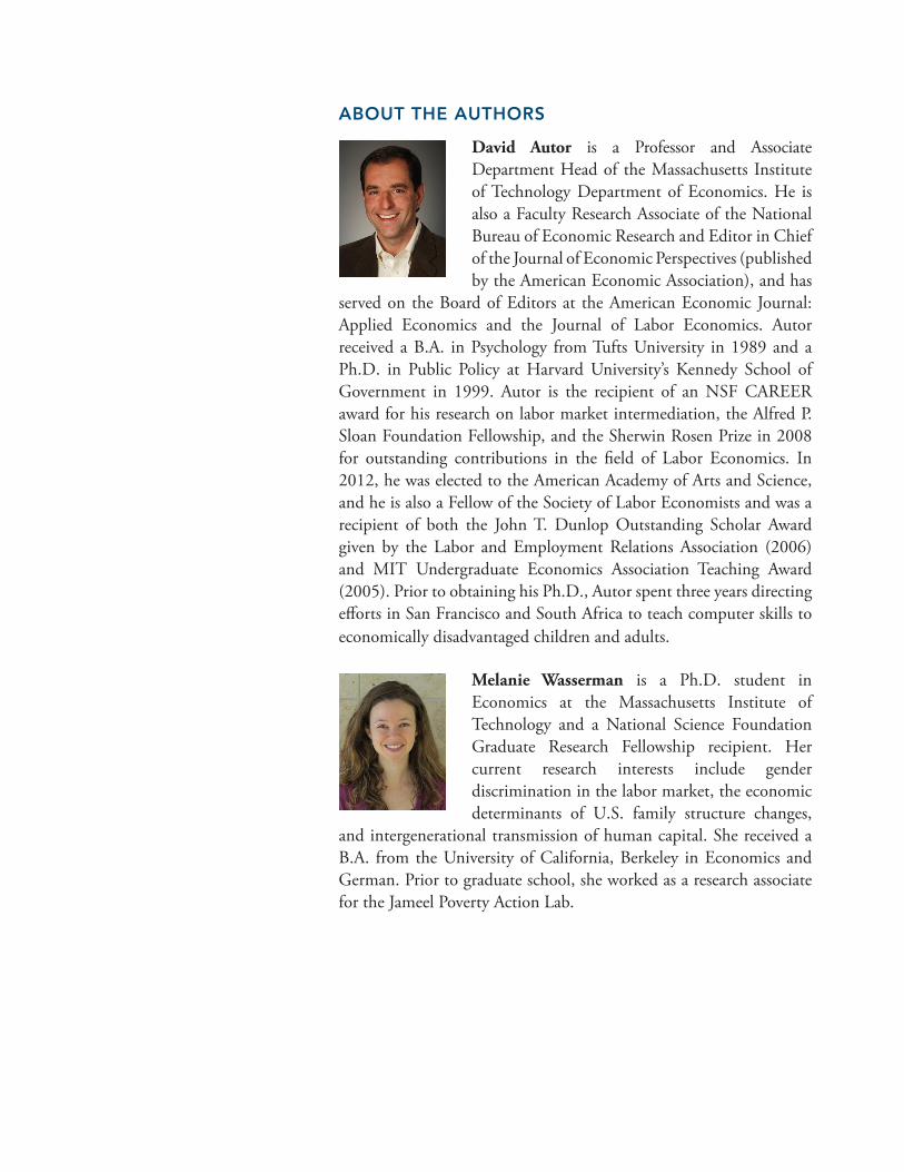
ABOUT THE AUTHORS
David Autor is a Professor and Associate Department Head of the Massachusetts Institute of Technology Department of Economics. He is also a Faculty Research Associate of the National Bureau of Economic Research and Editor in Chief of the Journal of Economic Perspectives (published by the American Economic Association), and has
served on the Board of Editors at the American Economic Journal: Applied Economics and the Journal of Labor Economics. Autor received a B.A. in Psychology from Tufts University in 1989 and a Ph.D. in Public Policy at Harvard University’s Kennedy School of Government in 1999. Autor is the recipient of an NSF CAREER award for his research on labor market intermediation, the Alfred P. Sloan Foundation Fellowship, and the Sherwin Rosen Prize in 2008 for outstanding contributions in the field of Labor Economics. In 2012, he was elected to the American Academy of Arts and Science, and he is also a Fellow of the Society of Labor Economists and was a recipient of both the John T. Dunlop Outstanding Scholar Award given by the Labor and Employment Relations Association (2006) and MIT Undergraduate Economics Association Teaching Award (2005). Prior to obtaining his Ph.D., Autor spent three years directing efforts in San Francisco and South Africa to teach computer skills to economically disadvantaged children and adults.
Melanie Wasserman is a Ph.D. student in Economics at the Massachusetts Institute of Technology and a National Science Foundation Graduate Research Fellowship recipient. Her current research interests include gender discrimination in the labor market, the economic determinants of U.S. family structure changes,
and intergenerational transmission of human capital. She received a B.A. from the University of California, Berkeley in Economics and German. Prior to graduate school, she worked as a research associate for the Jameel Poverty Action Lab.


![Wayward Children EZEK. 18:10-13 [By Ron Halbrook]](https://img.pdfslide.us/doc/110x75/56649cf55503460f949c4a32/wayward-children-ezek-1810-13-by-ron-halbrook.jpg)