PHYSICS OF FLUIDS 26, 027105 (2014)

Wave–vortex interactions in the nonlinearSchrodinger equation

Yuan Guoa) and Oliver BuhlerCourant Institute of Mathematical Sciences, New York University, New York,New York 10012, USA

(Received 13 October 2013; accepted 3 February 2014; published online 21 February 2014)

This is a theoretical study of wave–vortex interaction effects in the two-dimensionalnonlinear Schrodinger equation, which is a useful conceptual model for the limitingdynamics of superfluid quantum condensates at zero temperature. The particularwave–vortex interaction effects are associated with the scattering and refraction ofsmall-scale linear waves by the straining flows induced by quantized point vorticesand, crucially, with the concomitant nonlinear back-reaction, the remote recoil, thatthese scattered waves exert on the vortices. Our detailed model is a narrow, slowlyvarying wavetrain of small-amplitude waves refracted by one or two vortices. Weakinteractions are studied using a suitable perturbation method in which the nonlinearrecoil force on the vortex then arises at second order in wave amplitude, and iscomputed in terms of a Magnus-type force expression for both finite and infinitewavetrains. In the case of an infinite wavetrain, an explicit asymptotic formula forthe scattering angle is also derived and cross-checked against numerical ray tracing.Finally, under suitable conditions a wavetrain can be so strongly refracted that itcollapses all the way onto a zero-size point vortex. This is a strong wave–vortexinteraction by definition. The conditions for such a collapse are derived and thevalidity of ray tracing theory during the singular collapse is investigated. C© 2014 AIPPublishing LLC. [http://dx.doi.org/10.1063/1.4865837]

I. INTRODUCTION

Wave–vortex interactions are a classical topic in fluid dynamics, with well-known applicationsincluding vortices created by dissipating sound waves as in acoustic streaming and the so-called“quartz wind,”1 longshore currents and rip currents created by breaking surface waves on beaches,2

or the micro-mixing of fluid droplets based on stirring by waves.3 Arguably, the field in which therelevant interaction theory is most advanced is that of atmosphere ocean fluid dynamics, becausethere it is well recognized that the nonlinear interactions between unresolved small-scale wavesand the resolved large-scale mean flow are crucial for the long-term dynamics of the system, andtherefore are crucial to climate prediction. This has led to a very detailed study of many wave–meaninteraction effects in this field, accounts of which can now be found in standard textbooks andresearch monographs.4–6

Another physical scenario in which wave–vortex interactions are well known to be clearlyimportant is the quantum superfluid dynamics of dilute Bose–Einstein condensates, in which there arelively interactions between various forms of dispersive waves and the peculiar quantum line vorticesthat allow the superfluid fluid component to perform a kind of vortex dynamics that in many waysis closely analogous to that of classical line vortices in incompressible fluid dynamics.7–9 Of course,a detailed description of quantum superfluid dynamics at finite temperature is a complicated field-theoretic affair, which goes significantly beyond fluid dynamics.10 Still, going back to the pioneeringwork of Landau,26 there are practically useful two-fluid models, in which an intimate mixture of

a)Email: yuanguo@cims.nyu.edu

1070-6631/2014/26(2)/027105/22/$30.00 C©2014 AIP Publishing LLC26, 027105-1

027105-2 Y. Guo and O. Buhler Phys. Fluids 26, 027105 (2014)

a “normal” and a “super” fluid component joined together through various coupling mechanismsis considered. However, the complexity of these two-fluid models11, 12 makes it somewhat hard toextract fundamental fluid-dynamical information from them, especially as the coupling mechanismin them are themselves models for more microscopic, fundamental wave–vortex interactions.

A special conceptual place is therefore reserved for the very simple but powerful superfluidmodels based on the (defocusing) nonlinear Schrodinger equation (NLS), also known as the Gross–Pitaevskii equation in this field.13, 14 Whatever the context, the NLS equation has a well-known fluid-dynamical interpretation via the Madelung transformation, which allows comparing and contrastingclassical and quantum fluid dynamics on an even footing.15 Strictly speaking, the NLS equation canonly model the Bose–Einstein condensate, which is closely related to superfluid behaviour16 at zerotemperature, but as a model for this limiting case it is of striking simplicity. Moreover, the NLSequation appears as a model equation in many other fields, ranging from nonlinear fibre optics tomodulated surface waves, so fundamental studies of its intrinsic dynamical behaviour are valuablein its own right. This motivated the present study.

The particular wave–vortex interactions considered here are two-dimensional problems in whicha slowly varying wavetrain of linear waves is scattered due to refraction by the straining flow inducedby point vortices, which are located at a large distance from the wavetrain. In particular, we computeboth the scattering of the linear waves as well as the concomitant nonlinear back-reaction ontothe vortices that arises at second order in wave amplitude, and which manifests itself as a certainsideways advection of the vortex by a wave-induced mean flow. This builds on an earlier study intwo-dimensional classical compressible fluid dynamics reported in Buhler and McIntyre17(hereafterreferred to as BM03),17 in which this novel interaction effect was called the remote recoil. Thepresent setting with the NLS equation differs in several important aspects from this earlier study, inwhich the wave dynamics was restricted to non-dispersive acoustic waves and in which the vorticesin question were compactly supported, but finite-sized patches of vorticity. In contrast, in the NLSequation the waves are strongly dispersive and the vortices are necessarily point vortices of zerosize. This necessitates a significant adjustment of the tools required to study this process.

Our main theoretical result is a description of the detailed wavenumber-dependence of thewave scattering process as well as of the concomitant recoil felt by the point vortices. Moreover,there is a novel possibility of extremely strong wave refraction by the point vortex that leads to asingular collapse of the wavetrain all the way into the location of the point vortex. The possibilityof such a wavetrain collapse in classical acoustic problem had been noted long ago,18 but only inthe NLS equation can the collapse proceed all the way to the zero-size vortex line. We investigateapproximately the linear wave dynamics of this fascinating wave collapse case in the NLS equation,but we were not able to compute the nonlinear wave–vortex interaction in this singular case. Somespeculations as to what these interactions might be based on experience with classical fluid dynamicsare offered in Sec. VII.

The paper is organized as follows. In Sec. II, governing equations are derived and the standardray-tracing theory is summarized. Sec. III gives the setup for a finite wavetrain scattered by a singlevortex and Sec. IV extends this to the scattering of infinite wavetrains. Theoretical results are derivedand cross-checked by numerical integration of ray-tracing equations. Sec. V then expands the resultsto situations with multiple vortices. Sec. VI contains a study of rays being trapped by a vortex andSec. VII offers concluding remarks.

II. GOVERNING EQUATIONS AND LINEAR WAVES

A. Nonlinear Schrodinger equation

The (defocusing) NLS, also called the Gross–Pitaevskii equation, is a well-known idealizedmodel for the dynamics of a quantum system of weakly interacting identical bosons near absolute zerotemperature, such as dilute Bose–Einstein condensates,9, 13 which are often realized experimentallyusing alkali gases.

The equation governs the complex-valued wave function ψ defined such that |ψ |2 is the numberdensity of the particles. Our detailed analysis will be in two space dimensions, but the general

027105-3 Y. Guo and O. Buhler Phys. Fluids 26, 027105 (2014)

equations hold in any number of spatial dimensions. In dimensional form, the NLS is

i�∂ψ

∂t= − �

2

2m∇2ψ + [U0|ψ |2 + V ]ψ, (1)

where � is Planck’s constant divided by 2π , U0 is a positive constant modeling particle repulsion, m isthe mass of a particle, and V (x, t) is an external potential, which we choose as V = −U0n0(1 + ϕ)with n0 being the density |ψ |2 at infinity and ϕ being a forcing potential discussed later. Thedimensional healing or coherence length9 is defined by

ξ = �√mn0U0

. (2)

It is the characteristic length over which the density relaxes from zero at solid walls or vortexlocations to its background value n0.

All the dimensional parameters can be eliminated by using non-dimensional variables. Forexample, denoting non-dimensional variables with a prime we may choose

x = �√mn0U0

x ′ = ξ x ′, t = �

n0U0t ′, and ψ = √

n0ψ′. (3)

Dropping the primes, the non-dimensional NLS equation is

i∂ψ

∂t= −1

2∇2ψ + (|ψ |2 − 1)ψ − ψϕ. (4)

If ϕ = 0, then the following integrals for mass, momentum, and energy are conserved:

N =∫

|ψ |2dx, P =∫

Im(ψ∗∇ψ)dx, (5)

and E =∫ {

1

2|∇ψ |2 + 1

2(|ψ |2 − 1)2

}dx. (6)

Here, * denotes complex conjugation. If ϕ �= 0, then the mass is still conserved, but the momentumand energy may change as described in (14) below.

B. Madelung transformation

The well-known Madelung transformation19 allows a fluid-dynamical interpretation of the NLSequation, but the physical nature of the “fluid” of course depends on the specific application at hand.In the present context, there is an actual fluid present, namely, the dilute Bose–Einstein condensate,so here the interpretation is straightforward. The transform is based on the polar representation

ψ = √h exp(iθ ), (7)

where h(x, t) ≥ 0 and θ (x, t) are real-valued functions describing the particle density and the phaseof the wave function, respectively. In terms of h = |ψ |2 and the velocity vector

u = ∇θ = Im(ψ∗∇ψ)

|ψ |2 , (8)

the three integrals in (6) become

N =∫

h dx, P =∫

hu dx,

and E =∫ (

h

2|u|2 + |∇h|2

8h+ (h − 1)2

2

)dx. (9)

027105-4 Y. Guo and O. Buhler Phys. Fluids 26, 027105 (2014)

Substituting (7) into (4) and separating real and imaginary parts yields

∂h

∂t+ ∇ · (hu) = 0 (continuity equation), (10)

∂θ

∂t+ |u|2

2+ (h − 1) − ϕ = ∇2

√h

2√

h= −

( |∇h|28h2

− ∇2h

4h

). (11)

Taking the gradient of (11) one obtains the associated momentum equation

∂u∂t

+ (u · ∇)u + ∇(h − 1) + ∇( |∇h|2

8h2− ∇2h

4h

)= F (12)

with the body force F = ∇ϕ. The third term is similar to the pressure gradient term in shallowwater equation while the fourth term known as “quantum pressure” resembles the effect of surfacetension. However, it needs to be borne in mind that the definition of u as the gradient of θ impliesthat the constraint

∇ × u = 0 (13)

holds in all regions where ψ �= 0. This constraint can be circumvented pointwise at vortex locations,where ψ = 0. We will use the transformed equations (10), (12), and (13) as the governing equationsfrom now on.

Finally, we may also note the exact equations for momentum and energy in flux form as

∂(hu)

∂t+ ∇ ·

{huu + ∇h∇h

4h+

(h2

2− ∇2h

4

)I}

= h F, (14)

∂e

∂t+ ∇ ·

{eu + h2 − 1

2u − ∇2h

4u + ∇ · (hu)

4h∇h

}= hu · F. (15)

Here, the energy density e = h|u|2/2 + |∇h|2/(8h) + (h − 1)2/2 is the integrand in (9).

C. Linear waves and ray tracing

The transformed equations will be studied with a regular perturbation expansion to second orderin a suitable small-wave-amplitude parameter a � 1, i.e., there will be a (steady) O(1) backgroundflow {U, H}, O(a) linear waves {u′, h′}, and an O(a2) nonlinear mean-flow response to the waves.Eventually, we will assume that the waves form a slowly varying wavetrain, which allows averagingand the use of ray-tracing theory. Of course, one could also perform the perturbation expansion interms of the wave function ψ in the original, untransformed NLS equation. For example, to O(a)accuracy the asymptotic relations u ∼ U + u′ and h ∼ H + h′ are consistent with ψ ∼ � + ψ ′,say, provided that � = √

H exp(iα) and ψ ′/� = h′/2H + iθ ′, where θ ∼ α + θ ′ such that U = ∇α

and u′ = ∇θ ′ hold. However, it is much easier to study the nonlinear interplay between waves andvortices at O(a2) in the fluid variables, which is why we proceed in this manner.

Now, the full O(a) equations for u′ and h′ are

∂h′

∂t+ ∇ · (H u′ + h′U) = 0, (16)

∂u′

∂t+ (U · ∇)u′ + (u′ · ∇)U + ∇h′

−1

4∇

[∇2

(h′

H

)]− 1

4∇

[∇H

H· ∇

(h′

H

)]= F′. (17)

Here, the irrotational linear force F′ serves to represent wave emission and absorption. We willonly solve these equations using the standard ray-tracing approximation, which is valid for a slowlyvarying wavetrain in a slowly varying background environment. Hence, we assume that the linearfields are given by the real part of the product between a slowly varying amplitude function and the

027105-5 Y. Guo and O. Buhler Phys. Fluids 26, 027105 (2014)

rapidly varying oscillatory function exp (i). Here, the rapidly varying wave phase is not to beconfused with the phase θ of the original wave function ψ in (7)!

The derivatives of the wave phase define the local wavenumber vector and frequency in theusual way and both must satisfy the standard dispersion relation based on a uniform backgroundwith constant density H and constant velocity U

k = ∇, ω = −t , ω = ω + U · k, ω =√

Hκ2 + κ4

4. (18)

Here, k is the local wavenumber vector, ω is the absolute wave frequency, and the intrinsic frequencyω is given in terms of κ = |k| by the dispersion relation in (18). From now on we restrict totwo-dimensional dynamics such that x = (x, y) and k = (k, l). It then turns out that the dispersionrelation in (18) is identical to that of the shallow water equations with surface tension.20 Hence,for small wave numbers or long wavelengths, ω ≈ √

Hκ is a non-dispersive sound wave dispersionrelation, whereas for higher wave numbers or short waves, ω ≈ κ2/2, which in quantum mechanicsis the dispersion relation for free particles. This wave-number-dependent asymptotic behavior willbe seen to give rise to the wave-number-dependence of the wave scattering angle due to vortices(see Sec. IV), which is different from the simpler classical theory in BM03.17

The standard ray-tracing equations for x = (x, y) and k = (k, l) as functions of time alonggroup-velocity rays are given in terms of the absolute frequency function

(x, k, t) = ω + U · k =√

Hκ2 + κ4/4 + U · k (19)

by the standard Hamiltonian equations20

dxdt

= +∂

∂kand

dkdt

= −∂

∂x, (20)

where the time derivative along a ray is defined as

d

dt= ∂

∂t+ (cg ·∇) (21)

acting on slowly varying functions of (x, t). The group velocity cg is defined by

cg = (ug, vg) = dxdt

= cg + U = 2H + κ2

2ωk + U . (22)

For steady background fields, the ray-tracing equations imply that dω/dt = 0, i.e., the absolutefrequency is constant along any group-velocity ray. In addition, if the background flow has azimuthalsymmetry around the origin of the coordinate system, then there is another ray invariant, namely,

M = (r × k)z = lx − ky. (23)

This will be the case in Secs. III and VI below. The evolution of wave amplitude along a ray isgoverned by the conservation law for the wave action A at O(a2)21

∂(H A)

∂t+ ∇ · (H Acg) = H

ωu′ · F′, (24)

where

A = E

ωand E = u′2

2+ h′2

2H+ 1

8

∣∣∣∣∇(

h′

H

)∣∣∣∣2

(25)

is the wave energy per unit mass. The wave action is conserved in region where F′ = 0. For a steadyunforced wavetrain, (24) reduces to

∇ · (H Acg) = 0. (26)

A very important quantity in wave–mean interaction theory is the pseudomomentum vector6

p = kA = kE

ω(27)

027105-6 Y. Guo and O. Buhler Phys. Fluids 26, 027105 (2014)

per unit mass. For irrotational velocity fields and a slowly varying wavetrain,6 we also havep = h′u′/H. The pseudomomentum evolution can be shown to satisfy

∂(H p)

∂t+ ∇ · (H pcg) = H A

dkdt

+ h′ F′ = −H A∂

∂x+ h′ F′. (28)

Unlike wave action, pseudomomentum can be created or destroyed without forcing or dissipationprovided the background flow is inhomogeneous as measured by non-vanishing ∂ /∂x. Physically,this corresponds to wave refraction caused by non-uniform H or U: such refraction conserves waveaction but not pseudomomentum.

III. REMOTE RECOIL WITH A SINGLE VORTEX

We follow BM0317 and consider the refraction of a finite wavetrain passing a single vortex asdepicted in Fig. 1. The O(1) vortex is placed at the origin of the coordinate system and an O(a)wavetrain of finite length 2L is passing it at a distance D, with a � 1 being the small wave amplitude.We assume that L and D have comparable size and that both are large compared to the healing length,which is unity, so the waves are passing the vortex remotely. The word remotely is used to emphasisthat there is no physical overlap between the vortex and waves. To make the wavetrain length finite,we employ a suitably chosen linear force field F′ that generates and absorbs the waves in thelocations marked symbolically by the loudspeakers. There are two linked wave–vortex interactioneffects in this situation, as discussed in detail in BM03.17 First, the linear waves are refracted bythe non-uniform background vortex flow. Second, the vortex experiences a remote recoil, namely,the vortex is expected to move slowly to the left due to advection by a nonlinear O(a2) mean flowinduced by the finite wavetrain. Both effects combine to balance the global momentum budget.

The present superfluid situation differs in several important aspects from the classical fluidsituation studied in BM03.17 First, the strength of the vortex circulation cannot be chosen arbitrarilybut is quantized.22 Also, in BM0317 the vortex had a finite size whereas here it is necessarily a pointvortex. Second, here the dynamics of the linear waves depends on their wavelength whereas they

FIG. 1. A background vortex with circulation � = 2π is passed at a distance D � 1 by a finite train of waves that aregenerated and absorbed in the locations marked by the loudspeakers. The waves are refracted by the O(1) background vortexflow (dashed curves) and at the same time the vortex is exposed to an O(a2) large-scale return flow induced by the waves(solid curves). Specifically, the background velocity of the vortex pushes the waves toward decreasing y at the source andpulls them toward increasing y at the sink. To keep y = constant along the rays, the phase lines have to tilt slightly as indicated.This leads to tilted recoil forces RA and RB at the loudspeakers and to a compensating remote recoil RV at the vortex,see (29).

027105-7 Y. Guo and O. Buhler Phys. Fluids 26, 027105 (2014)

did not in BM03.17 Third, in BM0317 the vortex was held steady by a suitable holding force withnonzero curl and the integral over that holding force then provided the definition of the total recoilforce RV , say, that is felt by the vortex. Here, this is not possible because only irrotational forces canarise in the equations. However, we are free to imagine a thought experiment in which the vortex iskept fixed by covering the vortex region with a small cylinder, say, and keeping the cylinder steadyby some external holding force, thereby allowing the background flow to remain steady. We identifythis holding force with (minus) the vortex recoil force RV , and we calculate it by integrating themomentum-flux equation (14) over a suitable control volume, which we take to be the large circler = D/2. On this circle the flow is unforced and steady, the wave field is zero and the height fieldis close to its undisturbed value, which is unity. The momentum flux across the circle must thenbalance the holding force on the imagined cylinder. Specifically, we define the exact recoil force by

RV = −∮

r=D/2

{huu · n + ∇h∇h

4h· n −

((h − 1)2

2+ h

2|u|2 + |∇h|2

8h

)n}

ds, (29)

where ds and n are the line element and outward normal on the large circle. This follows from (14)after eliminating a term containing ∇2h by using the steady unforced version of the Bernoulli theoremin (11) and discarding an irrelevant constant. As we shall see, this extra step greatly simplifies theperturbation expansion of the integral.

A. Background flow

The background vortex is a point vortex located at the coordinate origin and its associatedvelocity field is axisymmetric with circumferential velocity U (r ) = �/(2πr ), where � > 0 is thecirculation. Because U is the gradient of the phase of a single-valued wave function, the circulationof the vortex is necessarily quantized as � = 2kπ, k ∈ Z. Higher-order vortices are unstable and arelikely to split into several first-order vortices. We will consider � = 2π in detail but retain a general� in some of the expressions below. The background velocity field is

U = (U, V ) = �

2π

(−y

r2,+x

r2

)=

(−y

r2,+x

r2

). (30)

The density field H(r) goes to zero at the vortex location r = 0 and it asymptotes toward unity forlarge r. Specifically, in the far field r � 1 the density profile H is well approximated23 from theBernoulli equation by

H (r ) ∼ 1 − U 2(r )

2= 1 − 1

2r2. (31)

For intermediate values of r, the shape of H(r) is easily found numerically and, if wanted, a uniformlyaccurate expression for H(r) is readily provided by the Pade approximation24

H (r ) ≈(

1116 + 11

96r2)

r2

1 + 23r2 + 11

96r4. (32)

This is illustrated in Fig. 2. As in BM03,17 a suitable small parameter measuring the remoteness ofthe wave–vortex interaction is

ε = |�|2π D

= 1

D� 1. (33)

Now there are two small parameters, a � 1 for wave amplitude and ε � 1 for vortex remoteness.It is necessary that ε � a such that the O(ε) background vortex can still be considered as a largebackground flow compared with the O(a) linear waves. Notably, the far-field approximation (31) iscorrect to O(ε2) on the circle r = D/2 in (29), and ∇H = O(ε3) there.

027105-8 Y. Guo and O. Buhler Phys. Fluids 26, 027105 (2014)

0 1 2 3 4 5−0.2

0

0.2

0.4

0.6

0.8

1

1.2

r

H(r

)

numericalPadefar−field

FIG. 2. Density field H(r) of a single vortex. The solid line is the numerical solution, the dashed line is the Pade approximationin (32), and the dotted line is the far-field approximation in (31).

B. Linear waves

There is no general analytical method for solving the ray-tracing equations in the case of strongbackground flow gradients. However, as in BM03,17 we will exploit the fact that these gradients areweak, of O(ε), along rays if the waves pass the vortex remotely. For example, this allows using thefar-field approximation (31) to obtain the absolute frequency function up to O(ε2) in the form

ω = ω + U · k ≈√

κ2 + κ4

4+ U · k − 1

4

U 2√1 + κ2/4

κ. (34)

Here, κ still needs to be computed along the ray, of course. The absolute group velocity function tothe same approximation is

cg = cg + U ≈ 2 + κ2

2√

κ2 + κ4/4k + U − U 2

4

κ2(κ2 + κ4/4

)3/2 k. (35)

We will assume that ω has the same value on all rays, which is consistent with a normal-modeapproach. Now, the ray-tracing equations are still difficult to solve even truncated to O(ε2). We willagain follow BM0317 and arrive at a useful wave solution by exploiting two important facts. First, itwill turn out that knowing the wave field to O(εn) is enough to find the recoil force to O(εn + 1). Forinstance, ignoring the effect of the vortex for the wave structure is sufficient to compute the recoilforce to O(ε), and using a first-order, O(ε) approximation for the waves is sufficient to computethe recoil force to O(ε2). We will therefore be content if we can compute the wave field correctlyonly up to O(ε). At this level of approximation the far-field height field is simply H ∼ 1 and theproblem reduces to ray tracing through a weak irrotational incompressible mean flow. Here, weexploit the second fact, namely, we use the extension to dispersive waves6, 25 of the classical26 resultthat non-dispersive wave rays through an irrotational incompressible flow are straight lines to O(ε).This result means that while k and hence the intrinsic group velocity cg are changed by refraction dueto U, the absolute group velocity cg remains pointing in the same direction. Hence, if the wavemakeron the left is slightly tilted toward the vortex to make vg = 0 at the source, vg = 0 will continueto be zero along the ray, i.e., the ray is just y = const. As in BM03,17 by combining this argumentwith the general constraint ∇ × k = 0 and evaluating (35) to O(ε), the wavenumber vector to O(ε)is easily computed to be

k = (k0, 0) − 2ω0

2 + k20

U, with ω0 =√

k20 + k4

0

4. (36)

027105-9 Y. Guo and O. Buhler Phys. Fluids 26, 027105 (2014)

The corresponding absolute group velocity to O(ε) is

cg = U + 2H + κ2

2ωk =

(2 + k2

0

2ω0k0 + 8

(2 + k20)(4 + k2

0)U, 0

)(37)

and then the corresponding wave action density A follows from (26) with H = 1, which reduces toconstant Aug along rays away from the wave source or sink. The result to order O(ε) is

A(x, y) = As(y)

(1 + �

2πγ

y(L2 − x2)

(x2 + y2)(L2 + y2)

)χx∈[−L ,L]. (38)

Here, χ is the characteristic function and As(y) is the wave action profile across the wave train atthe wave source or sink, which are equal by symmetry here. This wave action expression omits finedetails such as the smooth matching to zero underneath the wave source and sink, but these finedetails will not be relevant for the recoil computation. Finally, the parameter γ depends on k0 via

γ = (2 + k20)2(4 + k2

0)

16ω0k0 =

(1 + k2

0

2

)2√

1 + k20

4. (39)

Note that γ ∼ k50/8 if k0 is large and that γ ∼ 1 if k0 is small, which is the shallow-water limit of

BM03.17

C. Mean-flow response

We define the mean flow by averaging over the rapidly varying wave phase in the usual wayand denote the averaging process by an overbar, so, for example, u is the mean velocity andu′ = 0. The background flow is part of the mean flow and the leading-order nonlinear mean-flowresponse arises at O(a2). By the assumptions 1 � ε � a, it is convenient to introduce the followingnotations to distinguish the contributions at different powers of a and ε. A single subscript denotesthe contribution at the corresponding power of a while a second subscript, if present, denotes thecontribution at corresponding power of ε, thus

h = H + h20 + h21 + h22 + · · · , (40)

u = U + u20 + u21 + u22 + · · · . (41)

This is also the relevant expansion of the complete flow field (h, u) needed for the integral in (29),simply because the wave field is zero on r = D/2. It is now easy to verify by inspection that, assaid before, to obtain the recoil force RV from (29) at O(a2ε) requires only the wave fields and themean-flow response to zeroth order in ε. In fact, only u20 is needed in the integral because H ≈ 1and therefore h20 does not contribute to (29) at O(a2). Two terms contribute at O(a2ε), which can becombined using a vector identity to yield

RV = −∮

r=D/2u20 × (U × n) ds = − �

2πz ×

∫ 2π

0u20|r= D

2dθ. (42)

To find u20, we combine the constraint ∇ × u20 = 0 with the average of the continuity equation (10)at O(a2), which for a steady mean flow is

U · ∇h2 + ∇ · (H u2) = −∇ · (h′u′). (43)

At zeroth order in ε, this implies

∇ · u20 = − 1

H∇ · (h′u′) = −∇ · p20 = −k0

∂ A

∂x, (44)

and now u20 can be computed. Before doing this we note an important simplification of (42)that follows from the fact that the restriction of u20 to the disk r ≤ D/2 is both irrotational andnon-divergent, which means that the components of u20 are harmonic functions on this restriction:

027105-10 Y. Guo and O. Buhler Phys. Fluids 26, 027105 (2014)

∇2u20 = 0. Therefore, we can apply the mean-value property of harmonic functions to (42) and getthe exact simplification

RV = −� z × u20(0, 0). (45)

This shows that the effective recoil force RV at O(a2ε) is given by the usual Magnus forceexpression27 based on the value of the mean-flow response velocity at the vortex location. Now, u20

is computed from ∇ × u20 = 0 and (44) using the standard Green’s function as

u20(x, y) = 1

2π

∫ ∫(x − x ′, y − y′)

(x − x ′)2 + (y − y′)2

[−k0

∂ A

∂x(x ′, y′)

]dx ′dy′. (46)

One can apply action density expression (38) to zeroth order in ε and approximate the slowly varyingpre-factor in the integrand by its value at the source (sink). With (x, y) = (0, 0) this yields

u20(0, 0) ≈ −k0

π

(L , 0)

L2 + D2

∫ +∞

−∞As(y)dy. (47)

The recoil force at O(a2ε) is then given by

RV = yk0�

π

L

L2 + D2

∫ +∞

−∞As(y)dy. (48)

This is precisely the same as the classical fluids result (4.24) in BM03.17 The reason for this is thatthe wavenumber-dependent modulation of the action density A at O(ε) in (38) does not enter at thislevel of approximation. This will be different in Sec. IV, where wave scattering and recoil forces atO(a2ε2) are considered.

IV. SCATTERING WITH A SINGLE VORTEX

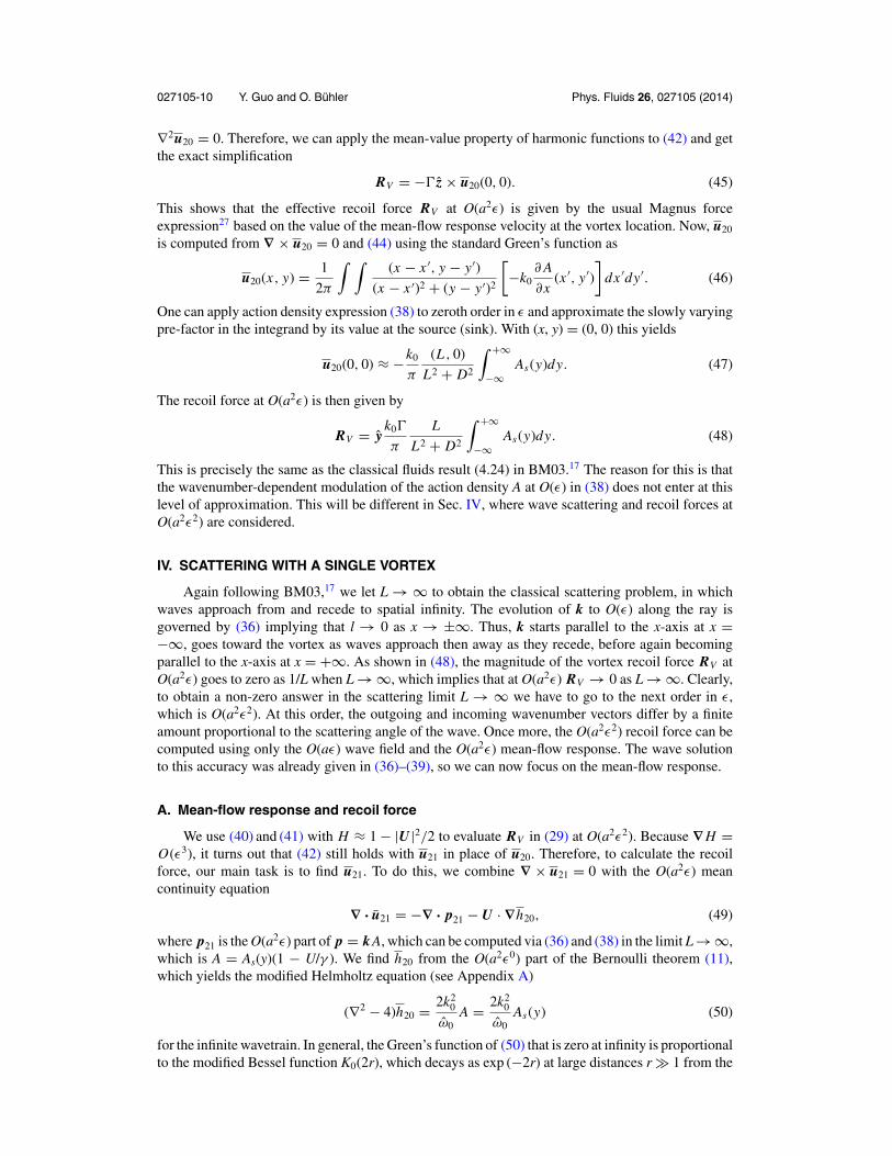
Again following BM03,17 we let L → ∞ to obtain the classical scattering problem, in whichwaves approach from and recede to spatial infinity. The evolution of k to O(ε) along the ray isgoverned by (36) implying that l → 0 as x → ±∞. Thus, k starts parallel to the x-axis at x =−∞, goes toward the vortex as waves approach then away as they recede, before again becomingparallel to the x-axis at x = +∞. As shown in (48), the magnitude of the vortex recoil force RV atO(a2ε) goes to zero as 1/L when L → ∞, which implies that at O(a2ε) RV → 0 as L → ∞. Clearly,to obtain a non-zero answer in the scattering limit L → ∞ we have to go to the next order in ε,which is O(a2ε2). At this order, the outgoing and incoming wavenumber vectors differ by a finiteamount proportional to the scattering angle of the wave. Once more, the O(a2ε2) recoil force can becomputed using only the O(aε) wave field and the O(a2ε) mean-flow response. The wave solutionto this accuracy was already given in (36)–(39), so we can now focus on the mean-flow response.

A. Mean-flow response and recoil force

We use (40) and (41) with H ≈ 1 − |U |2/2 to evaluate RV in (29) at O(a2ε2). Because ∇H =O(ε3), it turns out that (42) still holds with u21 in place of u20. Therefore, to calculate the recoilforce, our main task is to find u21. To do this, we combine ∇ × u21 = 0 with the O(a2ε) meancontinuity equation

∇ · u21 = −∇ · p21 − U · ∇h20, (49)

where p21 is the O(a2ε) part of p = kA, which can be computed via (36) and (38) in the limit L → ∞,which is A = As(y)(1 − U/γ ). We find h20 from the O(a2ε0) part of the Bernoulli theorem (11),which yields the modified Helmholtz equation (see Appendix A)

(∇2 − 4)h20 = 2k20

ω0A = 2k2

0

ω0As(y) (50)

for the infinite wavetrain. In general, the Green’s function of (50) that is zero at infinity is proportionalto the modified Bessel function K0(2r), which decays as exp (−2r) at large distances r � 1 from the

027105-11 Y. Guo and O. Buhler Phys. Fluids 26, 027105 (2014)

−20 −10 0 10 20−20

−10

0

10

20

x

y (s

cale

d)

−20 −10 0 10 20−20

−10

0

10

20

x

y (s

cale

d) k0 = 1

k0 = 2

k0 = 4

(b)(a)

FIG. 3. (a) Numerical ray-tracing results for k0 = 1 and various y0 = −D. Rays are started from |y0| = {5, 10, 20} withthe corresponding values for ε are {0.2, 0.1, 0.05}. The y-axis is rescaled by y0 + (y(t) − y0)/0.05 to show the scattering;(b) numerical ray-tracing results for ε = 0.1 (or |y0| = 10) and different k0. The initial wavenumber k0 are chosen to be {1,2, 4}. The y-axis is rescaled by y0 + (y(t) − y0)/0.02 to show the scattering.

source. This makes obvious that h20 is nonzero only in the vicinity of the wavetrain. Moreover, byassumption the action density A is slowly varying compared to the healing length, which is unity inour scaled variables, and therefore the solution of (50) inside r = D/2 is well approximated by theslowly varying expression

h20 = − k20

2ω0A = − k2

0

2ω0As(y) such that − U · ∇h20 = k2

0

2ω0V

d As

dy. (51)

The accuracy of (51) is discussed in more detail in Appendix B. We can now repeat the earlierargument and conclude that the components of u21 are harmonic on the restriction r ≤ D/2, andhence the recoil force at O(a2ε2) is again given by a Magnus formula, namely,

RV = −� z × u21(0, 0). (52)

Inverting (49) with ∇ × u21 = 0 then provides the velocity at the vortex as

u21(0, 0) = 1

2π

∫ ∫(−x,−y)

x2 + y2

[k0

γ

∂U

∂xAs(y) +

(2ω0

2 + k20

+ k20

2ω0

)V

d As

dy

]dxdy

= x�k0sgn(D)

16π D2

(1

γ+ k0

ω0+ (2 + k2

0)(4 + k20)

4γ

) ∫ +∞

−∞As(y)dy (53)

with γ given in (39). Consequently, the recoil force at O(a2ε2) for scattered waves is

RV = − y�2sgn(D)

16π D2

(1

γ+ k0

ω0+ (2 + k2

0)(4 + k20)

4γ

)k0

∫ +∞

−∞As(y)dy. (54)

The sign of the circulation does not matter for RV , but it does matter whether the waves pass to theright or the left of the vortex. We use D > 0 if the waves pass to the right, as exemplified by thelower rays in Fig. 3. Now, for small k0 the bracket in (54) goes to 4, which recovers the classicalshallow-water results in BM03.17 Moreover, in this limit k0 A = k0 E/ω0 → E and therefore at fixedwave energy density the recoil force goes to a nonzero limit as k0 → 0. Conversely, for large k0 thebracket goes to 4/k0, which means the recoil force becomes proportional to the action density A inthis limit. At fixed wave energy density E = ω0 A, this means the recoil force tends to zero as 1/k2

0as k0 → ∞.

B. Scattering angle and scale-selective refraction

From the recoil force at O(a2ε2), we can compute the global scattering angle θ∗ of the waves.As described in BM03,17 this is based on a global momentum budget argument, which gives anequality between −RV and the total rate of change of pseudomomentum. The starting point is the

027105-12 Y. Guo and O. Buhler Phys. Fluids 26, 027105 (2014)

expression of RV in (29). We will investigate the O(a2) terms in the limit r → ∞ where r comesfrom the line element ds = rdθ . It can be shown that (permitting H = 1 here)

RV = − limr→∞

∫ 2π

0

(u′u′ + 1

4∇h′∇h′

)· nrdθ = − lim

r→∞

∫ 2π

0pcg · nrdθ. (55)

This implies that the recoil force is equal to minus the difference between outgoing and incomingpseudomomentum fluxes, i.e., the recoil force is equal to minus the rate of change of pseudomo-mentum due to refraction by the vortex flow. The total wave action is conserved, hence the total rateof change of pseudomomentum is equal to the change in wavenumber vector times the total flux ofconserved wave action along the wavetrain

RV = −(k− − k+)(total wave action flux along wavetrain), (56)

where k− and k+ are the incoming and outgoing wavenumber vectors, respectively. We use (56) tocompute the scattering angle at O(ε2) and since the wavenumber vector change is O(ε2), the waveaction flux need only to be computed at leading order O(a2ε0), which is

total wave action flux along wavetrain = 2 + k20

2ω0k0

∫ +∞

−∞As(y)dy. (57)

Because of ray-invariance of absolute frequency, we have |k−| = |k+| and therefore

k− − k+ = θ∗ z × k− (58)

for small θ∗. Now using (54), (56), and (57) and k− = (k0, 0) we obtain the nice expression

θ∗ = πε2sgn(D)

{2

(2 + k20)3

+ 1

(2 + k20)2

+ 1

2 + k20

}. (59)

For small k0 this is consistent with the result θ∗ = πε2sgn(D) found in BM03.17 For larger k0 thescattering angle decrease sharply, as illustrated in Fig. 3. This should have notable consequences evenin less idealized situations. For example, this suggests that if a broadband wave field were to passthe vortex, then one should find that the small-wavenumber components have been preferentiallyscattered into the lee of the vortex.

C. Numerical ray-tracing results

Numerical results are presented to test the theoretical predictions by integrating the ray-tracingequations (20) numerically with a standard Runge–Kutta scheme. This is done without any explicitexpansion in ε � 1 although the density field is approximated by (31) such that ∇H = (x, y)/r4.This yields

dx

dt= 2H + κ2

2ωk + U = 2H + κ2

2ωk − �

2π

y

r2,

dy

dt= 2H + κ2

2ωl + V = 2H + κ2

2ωl + �

2π

x

r2,

dk

dt= − κ2

2ω

∂ H

∂x− Ux k − Vxl = − κ2

2ω

x

r4− �

2π

2xy

r4k − �

2π

y2 − x2

r4l,

dl

dt= − κ2

2ω

∂ H

∂y− Uyk − Vyl = − κ2

2ω

y

r4− �

2π

y2 − x2

r4k + �

2π

2xy

r4l.

(60)

The first column holds for any H and U while the second column uses H and U in (30) and (31). Theinitial conditions are x(0) = −∞ (or a large enough negative number), y(0) = −D, k(0) = k0 > 0,and l(0) = 0. Fig. 3(a) shows the results of a number of runs with varying y(0) = −D and fixedk0 = 1 with � = 2π . The figure is rescaled in the y-axis as described in the caption to highlightthe scattering angle. The symmetry between waves passing to the left or to the right of the vortexcan be observed. The scattering angle θ r was computed for various values of ε and compared withthe analytical predictions θ∗ from (59). The results are collected in Table I. The last column clearly

027105-13 Y. Guo and O. Buhler Phys. Fluids 26, 027105 (2014)

TABLE I. Scattering results for k0 = 1, � = 2π , and y0 = −D = −1/εis varied between runs. The predicted scattering angle θ∗ is from (59), theangle θ r comes from numerical integration of ray-tracing equations (60).The relative error Rel is defined by (θ∗ − θ r)/θ r.

D ε θ∗ θ r (θ∗ − θ r)/θ r Rel/ε

5 0.20 0.065 0.046 0.42 2.110 0.10 0.016 0.013 0.21 2.120 0.05 0.0041 0.0037 0.11 2.150 0.02 0.00065 0.00063 0.043 2.1

shows that the relative error scales as ε, which suggests that the next term in the expansion of θ∗would be ∝ε3. Such a term would break the symmetry between waves passing to the left or right ofthe vortex that holds at O(ε2).

Of course, what is special in superfluids is that the dispersion relation in (18) has differentasymptotic behaviour for small and large wavenumber, so the important task is to vary k0. Fig. 3(b)shows the results of a number of runs with varying k0 while ε is kept constant. Numerical results ofthe scattering angle θ r for various values of k0 and comparison with analytical predictions θ∗ from(59) are summarized in Table II. The last column suggests that the coefficient of the next term in theε-expansion of θ∗ might be proportional to 1/k0.

V. SCATTERING WITH MULTIPLE VORTICES

Our method also applies to scattering problem with multiple vortices. Similar to the singlevortex case, we can cover each vortex region with a small cylinder and keep the cylinder steady bysome external holding force. In this way, we can therefore assume n vortices are kept unmoved atlocation (xi, yi) with circulation �i. As mentioned earlier, the vortex is quantized as �i = 2kπ, k ∈ Zand is stable for k = ±1 only. In order to have similar small parameter as ε in the single vortex case,we assume all vortices are far away from the wavetrain and define

1 � εi = |�i |2π (yi + D)

= 1

yi + D� a, (61)

where all εi are of the same size, which is comparable to ε.

A. Theoretical prediction

Previous results (36), (38), (49), and (50) are still valid, except that we need to change thevelocity field U to

(U, V ) = U =n∑

i=1

U i =n∑

i=1

(Ui , Vi ) =n∑

i=1

�i

2π

(−(y − yi ), x − xi )

(x − xi )2 + (y − yi )2, (62)

TABLE II. Results for ε = 0.05, � = 2π , and k0 vary between runs. Thepredicted scattering angle θ∗ is from (59), the angle θ r comes from numericalintegration of ray-tracing equations (60). The relative error Rel is definedvia (θ∗ − θ r)/θ r.

k0 θ∗ θ r (θ∗ − θ r)/θ r Rel/ε

1 0.0041 0.0037 0.11 2.12 0.0016 0.0015 0.056 1.14 0.00046 0.00045 0.026 0.508 0.00012 0.00012 0.013 0.25

027105-14 Y. Guo and O. Buhler Phys. Fluids 26, 027105 (2014)

the superposition of the velocity fields induced by each vortex. Applying the inversion formula to(49) with the irrotational condition ∇ × u21 = 0 gives

u21(x j , y j ) = 1

2π

∫ ∫(x j − x, y j − y)

(x j − x)2 + (y j − y)2

×n∑

i=1

[k0

γ

∂Ui

∂xAs(y) +

(2ω0

2 + k20

+ k20

2ω0

)Vi

d As

dy

]dxdy (63)

with constants γ given in (39). Then following the Magnus force formula, total force felt by allvortices is

RV = −n∑

j=1

� j z × u21(x j , y j ), (64)

from which one can compute the scattering angle of the waves. To do this, we continue using theglobal momentum budget argument, which says the recoil force is equal to minus the rate of changeof pseudomomentum. Then by (56)–(58) the total recoil force is

RV = −θ∗ z × k−2 + k2

0

2ω0k0

∫ +∞

−∞As(y′)dy′. (65)

Combine (63) and (64) we obtain the scattering angle of the wavetrain

θ∗ =[

2

(2 + k20)3

+ 1

(2 + k20)2

+ 1

2 + k20

] {n∑

i=1

πε2i sgn(yi + D)

+∑i �= j

2�i� j

π2

∫(yi + D)(x ′ − xi )(x ′ − x j )

[(x ′ − xi )2 + (D + yi )2]2[(x ′ − x j )2 + (D + y j )2]dx ′

⎫⎬⎭ . (66)

The integral in the formula can be explicitly calculated since the integrant is an integrable rationalfunction. Detailed calculation can be found in Appendix C. Compared with the scattering anglefor a single vortex in (59), the scattering angle in multiple vortices case contains two parts: one isthe simple addition of the effects of every vortex with ε replaced by εi and D by D + yi, whileremains to be the distance between each vortex and the wavetrain; the other is the interactive effectbetween different vortices (the i-j term in the formula). Though a little weird, the interaction is notdifficult to understand: in (49) the mean-flow response u21 contains the contribution from all vorticesmanifested by the total velocity field U. Therefore, in addition to feeling itself’s mean-flow as in thesingle vortex case, each vortex is also in the responsive mean-flow induced by all other vortices.

B. Numerical results

As usual, we can numerically integrate the ray-tracing equations to double check our theoreticalprediction in (66). Since the wavetrain is far away from all vortices, we use the far-field approximatebackground density H in (31) which is

H = 1 − |U |22

hence ∇H = −(U ·∇)U (67)

by chain rule with U given in (62). Then the ray-tracing equations are given by the first equality in(60) with H and U following (62) and (67). To check the theoretical prediction θ∗, we focus on twohorizontal (vertical) vortices of equal distance from the origin with opposite (same) circulation. Ormore specifically, the vortex at (− xd, 0) or (0, xd) has circulation 2π in both cases while the one at(xd, 0) or (0, −xd) has circulation −2π for opposite circulation and 2π for same circulation case.The wavetrain starts from x(0) = −∞ (or a large enough negative number), y(0) = −D with initialwavevector k(0) = (k0, 0). Fig. 4 shows the results of a number of runs with varying y(0) = −D withall other parameters being kept constants. The figure magnifies the scattering angles by rescaling

027105-15 Y. Guo and O. Buhler Phys. Fluids 26, 027105 (2014)

−50−25 0 25 50−50

−25

0

25

50

y (s

cale

d)

−50−25 0 25 50−50

−25

0

25

50

y (s

cale

d)

−50−25 0 25 50−50

−25

0

25

50

y (s

cale

d)

−50−25 0 25 50−50

−25

0

25

50

y (s

cale

d)

(a) (b)

(c) (d)

x x

xx

FIG. 4. Numerical ray-tracing results for (a) two vortices with opposite circulation ±2π are at (−5, 0) and (5, 0). (b) Twovortices with positive circulation 2π are at (−5, 0) and (5, 0). (c) Two vortices with opposite circulation ±2π are at (0, 5)and (0, −5). (d) Two vortices with positive circulation 2π are at (0, 5) and (0, −5). The initial wavenumber is k0 = 2. Wavesare started from |y0| = {10, 20, 40}. The y-axis is rescaled by y0 + (y(t) − y0)/0.02 to highlight the scattering.

the y-axis as described in the caption. The symmetry between the left and right passing waves canbe easily observed, which corresponds to being quadratic in terms of � in (66).

We can also calculate the relative error by comparing the numerical and analytic results. Butunlike the single vortex case where the relative error is proportional to ε, there is no simple predictionof the next term in the asymptotic expansion because it also depends on the relative position of thewavetrain and all vortices.

VI. RAY COLLAPSE ONTO A VORTEX

If the waves get close to a vortex, then the interaction parameter ε is obviously not small anymoreand the previous scattering analysis does not apply. The extreme case is where the wave ray actuallyspirals into the vortex and collapses to its centre in finite time. Clearly, ray collapse is a drastic changefrom the previous weak scattering and weak wave–vortex interaction situation. Its possibility wasapparently first pointed out by Salant18 in the context of two-dimensional acoustic waves outside apoint vortex, with a later extension to three-dimensional acoustic waves by others.28, 29

We will investigate the possibility for ray collapse in the nonlinear Schrodinger equation byusing the NLS dispersion relation (70) below, and while taking the detailed density structure of thecore into account. Using standard methods, we will find the criterion for ray collapse and investigatethe structure of the collapsing rays. This is an extension of the earlier studies, which in their explicitresults were restricted to acoustic waves and constant core density, so the underlying dispersionrelation was ω = κ + U · k. As κ grows without bound during collapse, this inevitably fails to bea good approximation to the NLS dispersion relation (70), and this has significant consequencesfor the ray structure. We then discuss a necessary condition for ray tracing to remain valid even asthe ray collapses onto a vortex and finally consider the inevitable wave amplitude growth duringcollapse.

A. Ray collapse condition

We assume the stationary axially symmetric vortex flow introduced in (30) with � = 2π

U = Uφφ = �

2π

1

rφ = 1

rφ, H = H (r ). (68)

Since the ray can get arbitrarily close to the vortex, we use (32) or the numerical solution of theNLS equation to approximate the density field H(r). Here, r is the unit vector in the direction ofr = (x, y) while φ is the unit azimuthal vector complying with the right-hand rule. By this choice,

027105-16 Y. Guo and O. Buhler Phys. Fluids 26, 027105 (2014)

one can decompose the wavenumber vector locally into

k = κr r + κφφ. (69)

The Hamiltonian ray-tracing system (20) is integrable because it has two pairs of variables and alsotwo independent invariants, which are here given by absolute frequency

ω =√

Hκ2 + κ4/4 + U · k =√

Hκ2 + κ4/4 + κφ/r, (70)

and the z-component of the aforementioned “angular momentum” invariant

M = (r × k)z = lx − ky = rκφ. (71)

The previously studied acoustic case is included by setting H = 1 and ignoring the κ4 term in (70).Substituting (69) and (71) into (70) yields

ω =

√√√√H

(κ2

r +(

M

r

)2)

+ 1

4

(κ2

r +(

M

r

)2)2

+ M

r2(72)

or in terms of κ2r ,

κ2r = 2

√H 2 +

(ω − M

r2

)2

− 2H − M2

r2. (73)

Now, the standard argument for a collapse condition is based on the fact that r decreases along theray only if the intrinsic group velocity points inward, which means κr < 0. Hence, a wavepacket willcollapse onto the vortex if κr < 0 initially and if |κr| remains bounded away from zero for all valuesof r ≥ 0. Conversely, if κr goes through zero and changes sign, then the ray is simply scattered andescapes again to infinity. Therefore, the collapse condition is precisely the non-existence of a radiusr∗ ≥ 0 where κr = 0. Assuming κr = 0 in (72) yields

ω =√

HM2

r2∗+ 1

4

M4

r4∗+ M

r2∗(74)

and hence the ray collapses precisely if this equation has no real positive solution for r∗. Byconstruction the frequency ω is positive, but M may have either sign. As detailed in Appendix Dit is easy to extract the necessary conditions −2 ≤ M ≤ 0 for collapse from (74). In other words,collapsing rays must propagate intrinsically against the spinning direction of the vortex, and theazimuthal progression of the wave phase, which is the physical interpretation of M, must be fairlymodest and less than that of a mode-2 wave. The remaining condition on ω is found numericallyand the full result is shown in Fig. 5, which depicts a convex-shaped parameter region of collapsingrays in the Mω-plane. Fig. 6 illustrates the rays of several collapsing and non-collapsing wave rays,which cross-checks the theory in Fig. 5.

B. Comparison with acoustic rays

The structure of the collapsing rays in the present Schrodinger equation differs significantlyfrom those in the previously studied acoustic equations. To begin with, as Fig. 6 illustrates, hererays can collapse onto the vortex by winding around the vortex in either a prograde or retrogradedirection relative to the circulation sense of the vortex. This is in contrast with the acoustic case, inwhich the rays always wind in a prograde direction around the vortex. This occurs in the acousticcase because the azimuthal vortex velocity diverges as r → 0 and therefore the prograde vortex flowmust eventually dominate the intrinsic group velocity, which is bounded by the fixed acoustic wavespeed. Not so in the Schrodinger case, where the intrinsic group velocity for large κ is proportionalto κ , which by inspection of (70) and (72) obeys the scaling κ ∝ 1/r if M �= 0. Therefore, the intrinsicretrograde group velocity (assuming M < 0) and the prograde vortex flow Uφ = 1/r are comparablein the present case, which allows one or the other to dominate during the collapse. Specifically,retrograde collapse occurs if M < −1 for the unit vortex with Uφ = 1/r.

027105-17 Y. Guo and O. Buhler Phys. Fluids 26, 027105 (2014)

−2.5−0.2

−2 −1.5

0.2

−1

0.4

−0.5

0.6

0.8

0.5

1

1

1.2

0

ω

M

non−collapse region

collapse region

non−collapse region

C

A

B

(−2, 0.616)

FIG. 5. Collapse region based on the dispersion relation (70). The boundary consists of the straight lines M = 0 and M =−2 and the connecting lower curve, which has been found numerically. The right boundary M = 0 is included in the collapseregion, but not the others. For example, the lower-left point on the boundary is at (−2, 0.616), which satisfies (74) withturning radius r∗ = 1.383. Points A, B, and C correspond to the three panels in Fig. 6, respectively.

Another difference between the acoustic and the NLS case follows from the observation thatif M �= 0, then the intrinsic frequency ω ∝ 1/r2 and kφ ∝ 1/r in both cases, but kr ∝ 1/r2 in theacoustic case while kr ∝ 1/r in the NLS case. This means that in the acoustic case kr dominatesover kφ and hence the wavenumber vector always turns precisely into the vortex as r → 0, whereasin the NLS case kr and kφ are comparable and hence the wave crests come into the vortex with afinite angle of attack, which is a function of M. Finally, in both the acoustic and the NLS case therays make an infinite number of revolutions around the vortex before reaching r = 0, but only inthe acoustic case is the geometric length of the rays also infinite in any finite neighbourhood of thevortex. This is another repercussion of the asymptotically much faster intrinsic group velocity, andhence much more rapid collapse, in the NLS case compared to the acoustic case.

Of course, there are no true point vortices in any compressible fluid model such as the Navier-Stokes equations, for example, and hence there the actual, finite-size vortex structure must eventuallybe taken into account, which prohibits the strict collapse of acoustic rays onto a compressible vortex.The situation is different in the NLS equations, where true point vortices are natural and essentialcomponents of the dynamics. This warrants looking into the possible validity of ray tracing duringthe collapse in the NLS equations.

C. Validity of ray tracing during wave collapse

Ray tracing approximates linear wave theory under the assumption that the waves form a slowlyvarying wavetrain, so when ray tracing predicts a singular solution such as the formation of a wave

−1 0 1−1

−0.5

0

0.5

1

−2 0 2−2

−1

0

1

2

−1 0 1−1

−0.5

0

0.5

1

FIG. 6. A positive unit vortex is placed at (0, 0) and the circle r = 1/√

2 broadly marks the vortex core region, in which H ≤0.07. Three different rays are shown, with initial conditions corresponding to the three points in Fig. 5. All rays are started at(x, y) = (−5, 0). Left (point A): retrograde collapsing ray with M = −1.998, ω = 0.7373, and k = (0.6574, 0.3996). Middle(point B): non-rotating ray with M = −1.000, ω = 0.2913, and k = (0.2626, 0.2). Right (point C): prograde collapsing raywith M = 0, ω = 0.515, and k = (0.5, 0).

027105-18 Y. Guo and O. Buhler Phys. Fluids 26, 027105 (2014)

caustic, where neighboring rays intersect, then this prediction may merely indicate that ray tracinghas broken down, but not linear theory. On the other hand, ray tracing may remain valid all the wayto the caustic, which then implies a singularity even in the full linear theory. This kind of situation isprobably most familiar from the study of critical layers for dispersive waves, where ray tracing mayor may not remain valid as the critical layer is approached, depending on the details of the dispersionrelation.6 Of course, this is a partial analogy at best. For example, experience with dispersive causticsat critical layers shows that the travel time to reach those caustics is infinite, whereas the travel timefor collapsing waves to reach the vortex is decidedly finite.

In light of this difficult theoretical situation, we will simply consider here a necessary conditionfor the validity of ray tracing during wave collapse, which is that the slowly varying criterion κr �1 remains valid along the ray as r → 0. This criterion measures whether the distance to the vortexappears “large” compared to the local wavelength; it is also easy to show that during one wave periodthe fractional change along group-velocity rays of both ω and κ is proportional to 1/(κr)2 as r → 0.

First off, we notice the simple bound

rκ = r√

κ2r + κ2

φ ≥ r |κφ| = |M |, (75)

but the equality holds only when κr = 0, i.e., when the ray does not collapse. For collapsing rays(75) is not very sharp and we can improve on it. Specifically, near the vortex r � 1 and hence by(73) and the approximation for H(r) in (32) one can get

κ2 = 2

√H 2 +

(ω − M

r2

)2

− 2H = 2ω − 2M

r2+ O(r2) ⇒ κ2r2 ≥ −2M. (76)

This makes clear that ray tracing fails in the limiting case M = 0. As we know that for collapsingrays −2 < M ≤ 0, these bounds suggest that ray tracing has the best chance of remaining valid forrays with M close to the limiting case M = −2, in which case κr ≥ 2. Of course, this is merely afinite-size bound, but ray tracing is often found to be surprisingly accurate in practice even if slowlyvarying criterion is not strongly satisfied. Our tentative conclusion is therefore that for values of Mnear M = −2, the collapse observed in ray tracing probably indicates a singular absorption of waveseven in full linear theory.

This does raise further questions about collapsing waves that we unfortunately cannot answerhere. For example, we ran some numerical experiments in which we followed neighbouring raysinto the vortex in order to find out whether these rays will touch at some finite r > 0 and therebyform an external caustic, which would also invalidate ray tracing. Direct numerical integration of theray-tracing equations shows the distance between neighbouring rays decays linearly in r and doesnot indicate any external caustic, but this is far from conclusive.

D. Asymptotic wave amplitude evolution during collapse

We can work out the wave amplitude predicted from ray tracing via the standard procedureof assuming a steady wavetrain and considering an infinitesimal ray tube formed of neighbouringrays such that the cross-sectional width of the tube is given by w, say. The (unforced) wave actionconservation law (24) applied to the ray tube then yields

∇ · (H Acg) = 0 ⇒ H A|cg|w = const (77)

along the tube. Now, in order to make progress, we assume that as r → 0 the cross-sectional width w

scales with r in the simplest self-similar way, which is w ∝ r . (This appears almost inevitable giventhe azimuthal symmetry of the situation, where we could create a family of neighbouring collapsingrays by the simple device of rotating a single collapsing ray around the origin.) However, we alsoknow that |cg| ∝ 1/r , so the tendencies in these two terms cancel each other asymptotically in (77).This leads to the asymptotic structure of the action density as

H A = const ⇒ A ∝ 1/H ∝ 1/r2. (78)

027105-19 Y. Guo and O. Buhler Phys. Fluids 26, 027105 (2014)

Similarly, using κ ∝ 1/r and ω ≈ κ2/2, the pseudomomentum density p = kA and the wave energydensity E = ωA are found to diverge even faster as

| p| = κ A ∝ 1/(Hr ) ∝ 1/r3 and E ∝ κ2 A ∝ 1/(Hr2) ∝ 1/r4. (79)

The validity of linear theory depends on the smallness of a suitable non-dimensional wave amplitudethat measures the size of the ignored nonlinear terms against the size of the retained linear terms.The amplitude of nearly plane waves is typically given by the square root of |u′|2κ2/ω2 or of therelative depth disturbance h′2/H 2. Both lead to the same result in the present case, which using (25)is

amp2 ∝ |u′|2 κ2

ω2∝ E

ω

κ2

ω∝ A ⇒ amp ∝

√A ∝ 1/

√H ∝ 1/r. (80)

This divergence of the amplitude implies the breakdown of linear theory in some neighbourhood ofthe vortex location r = 0, which is quite consistent with the singular nature of the wave collapse.

VII. CONCLUDING REMARKS

Mutatis mutandis, our considerations of the remote recoil in the nonlinear Schrodinger equationhas followed closely the previous computations in classical acoustic fluid dynamics that weredescribed in BM03.17 For the refraction of the linear waves by isolated vortices, the most significantdifference was the wavenumber-dependence of the scattering process in the NLS system, whichdistinguished between the low-wavenumber regime, in which the classical acoustic results wererecovered, and the high-wavenumber regime, in which the scattering behaviour was very different.Using the NLS as a simple mean-field model for the quantum mechanics of a Bose–Einsteincondensate, the large-scale regime corresponds to collective particle motions while the small-scaleregime corresponds to individual particle motions.

As far as the concomitant nonlinear back-reaction on the vortices is concerned, the maindifference was that the use in BM0317 of a vortical holding force could not be transferred to theNLS equation, where external forces are necessarily irrotational. Instead, we employed the standardmethod of computing the momentum budget for a large control volume r = D/2 surroundingthe vortex, together with the observation that the O(a2) mean-flow response was harmonic onthe restriction to this control volume, which allowed the use of the averaging theorem for harmonicfunctions. This construction again facilitated computing the wave scattering angle from a momentumbudget, with results similar to the classical acoustic results in BM03.17

This contrasts with the phenomenon of collapsing rays onto a point vortex, which does not occurin classical acoustic fluids because there the vortex size is necessarily finite. Of course, the oppositerestriction is true in the NLS system, in which all vortices are line vortices, or point vortices in thepresent two-dimensional situation. As shown in Sec. VI D, such a wave collapse must inevitablybe accompanied by the divergence of the wave amplitude and therefore by a breakdown of lineartheory near the vortex. It is fascinating to speculate about the nonlinear wave–vortex interactionsthat might take place in this case. For example, it is well understood that a divergent wave amplitudein classical fluid dynamics would lead to wave dissipation via nonlinear wave breaking and theconcomitant generation of a dipolar mean-flow vorticity pattern at the edges of the breaking zone.30

In this process, the pseudomomentum of the waves is converted into the hydrodynamical impulseof the freshly created dipolar vorticity field.15 This kind of process is not exactly possible in theNLS equation because of its inherent restriction to point vortices, but it seems reasonable to expectthat bundles of point vortices can be formed by breaking waves in the NLS equation, mimickingthe analogous process in classical fluids and recovering the aforementioned conversion of wavepseudomomentum into vortical impulse. If this speculation is correct, then a collapsing wave raywould shower the original vortex with newly created vortex dipoles within a small wave breakingzone surrounding the original vortex! Investigating these strongly nonlinear aspects of the wave–vortex interactions in the NLS equation is of course outside the kind of theory we have availablehere.

027105-20 Y. Guo and O. Buhler Phys. Fluids 26, 027105 (2014)

Finally, we reiterate that real superfluid dynamics at finite temperature goes far beyond theNLS equation, even in the case of a dilute Bose–Einstein condensate. So from this point of viewit is questionable whether the effects we have described here have observable counterparts in suchsuperfluid systems. On the other hand, the NLS equation is a self-consistent and self-contained modelparadigm for many physical systems, ranging from classical wave envelope dynamics to quantummechanics, and therefore seeking to further our understanding of the intrinsic NLS dynamics isimportant in its own right.

ACKNOWLEDGMENTS

Financial support for Y.G. and O.B. under the U.S. National Science Foundation (NSF) GrantNos. DMS-1009213, 1312159 and OCE-1024180 is gratefully acknowledged. We also thank thehelpful comments from two anonymous referees for helping us improve the paper.

APPENDIX A: DEVIATION OF EQ. (50)

The Bernoulli equation (11) at O(a2) reads (let ϕ = 0)

(∇2 − 4)h20 = 2u′ · u′ + h′∇2h′ + |∇h′|22

. (A1)

We can write the linear fields explicitly by ψ ′/� = C1ei + C2e−i. Since we are only interested inthe O(a) waves, we can use the approximation H = 1. Therefore, the RHS of (A1) is

− 2κ2(C1C2 + C∗1 C∗

2 ) = 4κ2

(ω + κ2

2+ 1

)|C2|2, (A2)

and the O(a2) energy is

E = u′2

2+ h′2

2H+ 1

8

∣∣∣∣∇(

h′

H

)∣∣∣∣2

= 2ω2

(ω + κ2

2+ 1

)|C2|2. (A3)

With the definition of wave action A = E/ω, we can get Eq. (50), which is

(∇2 − 4)h20 = 2κ2

ω2E = 2κ2

ωA ≈ 2κ2

0

ω0As(y). (A4)

APPENDIX B: ACCURACY OF (51) IN DETERMINING u21

The exact solution of (50) is

h20 = − k20

2ω0

{∫ ∞

ye2(y−ξ ) As(ξ )dξ +

∫ y

−∞e−2(y−ξ ) As(ξ )dξ

}. (B1)

The difference between this exact solution and the approximate one in (51) will decay as−exp (−2|y + D|) away from the wavetrain y = −D, which is a very small number inside r ≤D/2. Moreover, the difference integrates to 0 when calculating u21.

APPENDIX C: INTEGRATION FOR MULTIPLE VORTICES

In (66), we need to calculate an integral of the form∫(x ′ − xi )(x ′ − x j )

[(x ′ − xi )2 + (D + yi )2]2[(x ′ − x j )2 + (D + y j )2]dx ′. (C1)

027105-21 Y. Guo and O. Buhler Phys. Fluids 26, 027105 (2014)

In order to simplify notation, let a = xi − xj, b = D + yi, and c = D + yj. Change variable using x= x′ − xi, (C1) reads ∫

x(x + a)

(x2 + b2)2[(x + a)2 + c2]dx . (C2)

According to partial fraction decomposition, the integrant can be written as

αx + β

(x2 + b2)2+ Ax + B

x2 + b2+ −Ax + C

(x + a) + c2(C3)

while each part can be integrated explicitly, giving the results

βπ

2b3sgn(b) + Bπ

bsgn(b) + (C + a A)π

csgn(c), (C4)

with the following constants:

F = a4 + 2a2b2 + b4 + 2a2c2 − 2b2c2 + c4,

α = (a3 + ab2 + ac2)/F, β = (a2b2 − b2c2 + b4)/F,

A = (a5 − 2a3c2 − 3ac4 + 2a3b2 + 2ab2c2 + ab4)/F2,

B = (−a6 − a4c2 + a2c4 + c6 − 2a4b2 − 4a2b2c2 − 2c4b2 − a2b4 − c2b4)/F2,

C = (−a6 + 5a4c2 + 5a2c4 − c6 − 2a4b2 + 2b2c4 − a2b4 − b4c2)/F2.

APPENDIX D: COLLAPSING CONDITION IN (M, ω) PLANE

We seek to find under what condition the equation

f (r ) =√

HM2

r2+ 1

4

M4

r4+ M

r2= ω (D1)

has a finite positive solution 0 < r < ∞ or not, the latter being the criterion for wave collapse. If M> 0, then

f (r ) → 0 as r → ∞ and f (r ) → ∞ as r → 0. (D2)

Therefore, by the intermediate value theorem, there is at least one finite r that satisfies (D1), so M ≤0 is a necessary condition for collapse. Similarly, if M < −2, then

f (r ) → 0 as r → ∞ and f (r ) >M2 + 2M

2r2→ ∞ as r → 0, (D3)

since the numerator is bigger than zero for M < −2. Hence, the necessary condition for collapse is−2 ≤ M ≤ 0. If M = 0, then f(r) ≡ 0 and therefore (D1) does not have a solution for any ω > 0, sothese rays will collapse. For −2 ≤ M < 0, let M = −αω so that (D1) reads

α

(√H

r2+ M2

4r4− 1

r2

)= 1. (D4)

We call the function inside the brackets g(r; M) and denote it maximum value over r by G(M) =max g(r; M), obtained at r = r*. To have the equality in (D4), the minimum value of α can take is

α∗(M) = 1

G(M). (D5)

This means, if α < α*, for any r > 0 the left-hand side in (D4) is always smaller than 1, i.e., there isno positive r satisfies (D4) or equivalently (D1). The wave packet will spiral in and finally collapseonto the vortex. For α > α*, there is some r > 0 satisfies (D4) and the wave packet will traveltoward the vortex till r = r and then begin leaving the vortex region — it would not collapse ontothe vortex. The maximum value G can be easily found numerically using the numerical density H(r)

027105-22 Y. Guo and O. Buhler Phys. Fluids 26, 027105 (2014)

and once known, using M = −αω, one arrives at the collapse condition in the Mω-plane shown inFig. 5.

1 J. Lighthill, Waves in Fluids (Cambridge University Press, 1978), p. 469.2 O. Buhler and T. E. Jacobson, “Wave-driven currents and vortex dynamics on barred beaches,” J. Fluid Mech. 449, 313

(2001).3 J. Vanneste and O. Buhler, “Streaming by leaky surface acoustic waves,” Proc. R. Soc. A 467, 1779–1800 (2011).4 R. Salmon, Lectures on Geophysical Fluid Dynamics (Oxford University Press, 1998), p. 362.5 G. K. Vallis, Atmospheric and Oceanic Fluid Dynamics: Fundamentals and Large-Scale Circulation (Cambridge University

Press, Cambridge, UK, 2006), p. 745.6 O. Buhler, Waves and Mean Flows (Cambridge University Press, 2009).7 R. Donnelly, Quantized Vortices in Helium II (Cambridge University Press, 1991).8 Quantized Vortex Dynamics and Superfluid Turbulence, Lecture Notes in Physics Vol. 571, edited by C. Barenghi, R.

Donnelly, and W. Vinen (Springer, 2001).9 C. J. Pethick and H. Smith, Bose-Einstein Condensation in Dilute Gases (Cambridge University Press, 2002).

10 A. J. Leggett, Quantum Liquids: Bose Condensation and Cooper Pairing in Condensed-Matter Systems (Oxford UniversityPress, Oxford, 2006), Vol. 34.

11 D. J. Thouless, P. Ao, and Q. Niu, “Transverse force on a quantized vortex in a superfluid,” Phys. Rev. Lett. 76, 3758(1996).

12 M. Stone, “Iordanskii force and the gravitational Aharonov-Bohm effect for a moving vortex,” Phys. Rev. B 61, 11780(2000).

13 N. G. Berloff, “Quantum vortices, traveling coherent structures and superfluid turbulence,” in Contemporary Mathematics:Stationary and Time Dependent Gross-Pitaevskii Equations, edited by A. Farina and J.-C. Saut (AMS, 2008), Vol. 473,p. 27.

14 S. G. L. Smith, “Scattering of acoustic waves by a superfluid vortex,” J. Phys. A 35, 3597 (2002).15 O. Buhler, “Wave-vortex interactions in fluids and superfluids,” Annu. Rev. Fluid Mech. 42, 205 (2010).16 F. London, “The λ-phenomenon of liquid helium and the Bose-Einstein degeneracy,” Nature (London) 141, 643 (1938).17 O. Buhler and M. E. McIntyre, “Remote recoil: A new wave-mean interaction effect,” J. Fluid Mech. 492, 207 (2003).18 R. F. Salant, “Acoustic rays in two-dimensional rotating flow,” J. Acoust. Soc. Am. 46, 1153 (1969).19 E. Madelung, “Quanten theorie in hydrodynamischer form,” Z. Phys. 40, 322 (1927).20 G. B. Whitham, Linear and Nonlinear Waves (Wiley-Interscience, 1974).21 F. P. Bretherton and C. J. R. Garrett, “Wavetrains in inhomogeneous moving media,” Proc. R. Soc. A 302, 529 (1969).22 L. Onsager, “Statistical hydrodynamics,” Nuovo Cimento Suppl. 6, 279 (1949).23 J. C. Neu, “Vortices in complex scalar fields,” Physica D 43, 385 (1990).24 N. G. Berloff, “Pade approximations of solitary wave solution of the Gross-Pitaevskii equation,” J. Phys. A 37, 1617

(2004).25 K. B. Dysthe, “Refraction of gravity waves by weak current gradients,” J. Fluid Mech. 442, 157–159 (2001).26 L. D. Landau and E. M. Lifshitz, Fluid Mechanics (Pergamon, 1987).27 E. B. Sonin, “Magnus force in superfluids and superconductors,” Phys. Rev. B 55, 485 (1997).28 S. V. Nazarenko, “Absorption of sound by vortex filaments,” Phys. Rev. Lett. 73, 1793 (1994).29 S. V. Nazarenko, N. J. Zabusky, and T. Scheidegger, “Nonlinear sound-vortex interactions in an inviscid isentropic fluid:

A two fluid model,” Phys. Fluids 7, 2407 (1995).30 O. Buhler, “On the vorticity transport due to dissipating or breaking waves in shallow-water flow,” J. Fluid Mech. 407,

235–263 (2000).