Embed Size (px)
Citation preview

Chapter 4
Waves I
In the last sections we have shown how we can build up a view of the motion of an oscillating
system by considering mass elements that oscillate along either a string or a spring-mass
system. It is then the superposition of all of the normal modes in these systems that de-
scribes the overall motions of the system. The motion in these systems is then dependent on
the initial conditions, and how many normal modes are active at the start of the oscillations.
In this section we move away from the discretised analysis of mass elements in a string
or spring system, and progress towards a completelt continuous description of waves.
4.1 The wave equation
4.1.1 The Stretched String
Consider a segment of string of constant linear density ⇢ that is stretched under tension T ,
as shown in Fig. 4.1.1.
Figure 4.1: Zoom in of a segment of a stretched string.
48

49
If we consider the net force acting on the string in both the vertical and horizontal
directions we find,
F
y
= T sin(✓ + �✓)� T sin ✓
F
x
= T cos(✓ + �✓)� T cos ✓.(4.1)
If we assume that �✓ is small, then
F
y
⇡ T �✓
F
x
⇡ 0,(4.2)
and expressing the force in terms of the linear density and the acceleration, we obtain
F
y
= ma
y
= (⇢�x)ay
= T �✓ = (⇢�x)@
2
y
@t
2
(4.3)
Note that here we have used the partial derivative, rather than the y, which implies
a normal derivative (d2y/dt2). This is because we know that the amplitude of the dsiplace-
ment in the y-direction is dependent on both the time t and the distance along the x-axis.
A lot of the work thaht follows will use partial di↵erential equations.
Fig. 4.1.1 also helps us to describe the relationship between the vertical displacement
and the position along the horizonal x axis.
For example, we can easily see that
tan ✓ =@y
@x
and@ tan ✓
@✓
= sec2 ✓ =@
2
y
@x@✓
therefore sec2 ✓@✓
@x
=@
2
y
@x
2
.
(4.4)
As before, if ✓ and �✓ are small, then sec ✓ ⇡ 1 and
sec2 ✓@✓
@x
⇡ �✓
�x
. (4.5)
Therefore,
�✓
�x
⇡ @
2
y
@x
2
and using Eq. 4.3,
=) @
2
y
@x
2
=⇢
T
@
2
y
@t
2
(4.6)
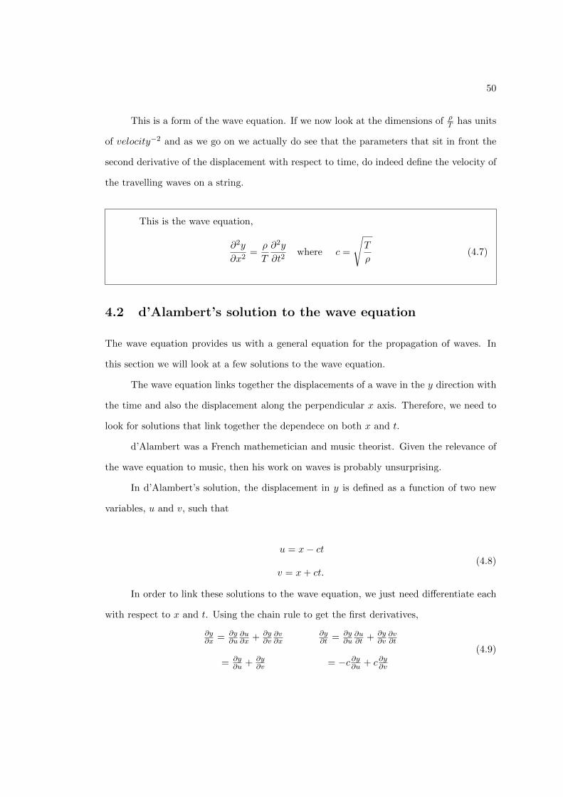
50
This is a form of the wave equation. If we now look at the dimensions of ⇢
T
has units
of velocity�2 and as we go on we actually do see that the parameters that sit in front the
second derivative of the displacement with respect to time, do indeed define the velocity of
the travelling waves on a string.
This is the wave equation,
@
2
y
@x
2
=⇢
T
@
2
y
@t
2
where c =
s
T
⇢
(4.7)
4.2 d’Alambert’s solution to the wave equation
The wave equation provides us with a general equation for the propagation of waves. In
this section we will look at a few solutions to the wave equation.
The wave equation links together the displacements of a wave in the y direction with
the time and also the displacement along the perpendicular x axis. Therefore, we need to
look for solutions that link together the dependece on both x and t.
d’Alambert was a French mathemetician and music theorist. Given the relevance of
the wave equation to music, then his work on waves is probably unsurprising.
In d’Alambert’s solution, the displacement in y is defined as a function of two new
variables, u and v, such that
u = x� ct
v = x+ ct.
(4.8)
In order to link these solutions to the wave equation, we just need di↵erentiate each
with respect to x and t. Using the chain rule to get the first derivatives,
@y
@x
= @y
@u
@u
@x
+ @y
@v
@v
@x
@y
@t
= @y
@u
@u
@t
+ @y
@v
@v
@t
= @y
@u
+ @y
@v
= �c
@y
@u
+ c
@y
@v
(4.9)

51
and the second derivatives,
@
2y
@x
2 = @
@x
⇣
@y
@u
@u
@x
+ @y
@v
@v
@x
⌘
@
2y
@t
2 = @
@t
⇣
@y
@u
@u
@t
+ @y
@v
@v
@t
⌘
=⇣
@
2u
@x@u
+ @
2v
@x@v
⌘
@y
@x
=⇣
@
2u
@t@u
+ @
2v
@t@v
⌘
@y
@t
using the equation for the first derivative (Eq. 4.9),
@
2y
@x
2 =�
@u
@x
@
@u
+ @v
@x
@
@v
�
⇣
@y
@u
+ @y
@v
⌘
@
2y
@t
2 =�
@u
@t
@
@u
+ @v
@t
@
@v
�
⇣
�c
⇣
@y
@u
� @y
@v
⌘⌘
Rearranging and substituting in the fact that (Eq. 4.8),
@u
@x
=@v
@x
= 1 and � @u
@t
=@v
@t
= c (4.10)
we find,
@
2y
@x
2 = @
2y
@u
2 + 2 @
2y
@u@v
+ @
2y
@v
2@
2y
@t
2 = c
2
⇣
@
2y
@u
2 � 2 @
2y
@u@v
+ @
2y
@v
2
⌘
. (4.11)
Substituting this in to the wave equation, we find that
@
2
y
@u@v
= 0.
We see that y is separable into functions of u and v,
=) y(u, v) = f(u) + g(v)
So the general solution to the wave equation is,
y(x, t) = f(x� ct) + g(x+ ct) (4.12)
Here, f and g are any functions of (x� ct) and (x+ ct), with the values determined
by the initial conditions.
4.2.1 Interpretation of d’Alambert’s solution
In the last section we found that the general solution to the wave equation (Eq. 4.7) is
provided by the linear combination of a function in (x� ct) and (x+ ct).
If we just focus on the f(x� ct) part of the solution, i.e.
y(x, t) = f(x� ct), (4.13)

52
then at time t = t
1
we have y(x, t1
) = f(x� ct
1
) and at time t
2
, y(x, t2
) = f(x� ct
2
). We
can rewrite this as
y(x, t2
) = f(x+ ct
1
� ct
2
� ct
1
)
= f([x� c(t2
� t
1
)]� ct
1
).
Looking at this equation in terms of what is happening physically, we can see that the
displacement at time t
2
and position x is equal to the displacement at time t
1
displaced by
a distance c(t2
� t
1
) to the left of x.
Therefore, the f(x� ct) solution describes a wave travelling to the right with velocity
c.
Figure 4.2: Motion of a triangle waveform for a solution with y(x, t) = f(x� ct). The wavemoves to the right with velocity c, therefore in time �t the wave moves a distance c�t tothe right.
Similarly, g(x+ ct) describes wave travelling to the left with velocity c.
4.2.2 d’Alambert’s solution with boundary conditions
In order to obtain a particular solution for any given system that is described by the wave
equation we have to consider the initial or boundary conditions of that system. Here we will
consider implementing boundary conditions for d’Alambert’s solution to the wave equation.
So we have,
y(x, t) = f(x� ct) + g(x+ ct).

53
Figure 4.3: Motion of a triangle waveform for a solution with y(x, t) = f(x+ ct). The wavemoves to the left with velocity c, therefore in time �t the wave moves a distance c�t tothe left.
At time t = 0 the wave has an initial displacement U(x) and velocity V (x), such that
y(x, 0) = U(x) = f(x) + g(x) (4.14)
Having one of the boundary conditions for the velocity should immediately alert us
to taking the derivative of y displacement with respect to t. Therefore,
@y(x, 0)
@t
= V (x) =@(x� ct)
@t
df
d(x� ct)+
@(x+ ct)
@t
dg
d(x+ ct)
= �c
d(x� ct)
dx
+ c
d(x+ ct)
dx
= �c
df(x)
dx
+ c
dg(x)
dx
.
(4.15)
Integrating this we find,
Z
df(x)
dx
� dg(x)
dx
= f(x)� g(x) = �1
c
Z
x
b
V (x).dx. (4.16)
Combining with Eq. 4.14,
g(x) =1
2U(x) +
1
2c
Z
x
b
V (x).dx
f(x) =1
2U(x)� 1
2c
Z
x
b
V (x).dx(4.17)
Therefore the solution would be,
54
y(x, t) =1
2[U(x� ct) + U(x+ ct)] +
1
2c
Z
x+ct
b
V (x).dx�Z
x�ct
b
V (x).dx
�
=1
2[U(x� ct) + U(x+ ct)] +
1
2c
Z
x+ct
x�ct
V (x).dx
(4.18)
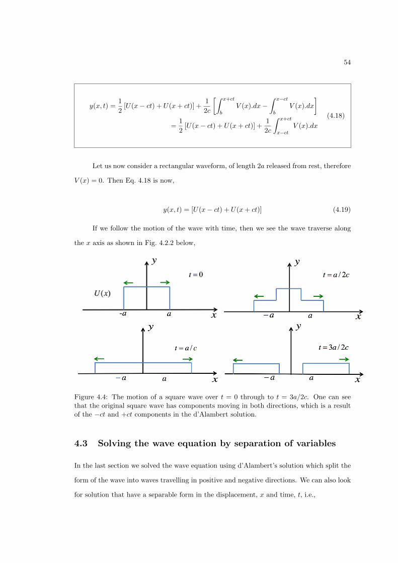
Let us now consider a rectangular waveform, of length 2a released from rest, therefore
V (x) = 0. Then Eq. 4.18 is now,
y(x, t) = [U(x� ct) + U(x+ ct)] (4.19)
If we follow the motion of the wave with time, then we see the wave traverse along
the x axis as shown in Fig. 4.2.2 below,
Figure 4.4: The motion of a square wave over t = 0 through to t = 3a/2c. One can seethat the original square wave has components moving in both directions, which is a resultof the �ct and +ct components in the d’Alambert solution.
4.3 Solving the wave equation by separation of variables
In the last section we solved the wave equation using d’Alambert’s solution which split the
form of the wave into waves travelling in positive and negative directions. We can also look
for solution that have a separable form in the displacement, x and time, t, i.e.,

55
y(x, t) = X(x)T (t) (4.20)
Substituting this solution into the wave equation (Eq. 4.7), we find
T (t)d
2
X(x)
dx
2
=1
c
2
X(x)d
2
T (t)
dt
2
=) X
X
=1
c
2
T
T
(4.21)
This equation can only be satisfied if both sides equal a constant, the so-called separation
constant.
T (t)d
2
X(x)
dx
2
=1
c
2
X(x)d
2
T (t)
dt
2
= C
(4.22)
We can consider general assumptions about the constants, i.e. positive, negative or
zero, to see what this means physically.
4.3.1 Negative C
So let us first consider the case where C is negative, such that C = �k
2.
d
2
X(x)
dx
2
= �k
2
X andd
2
T (t)
dt
2
= �(ck)2T.
These have a familiar form, in this case the 2nd derivative of the displacement and the time
terms are equal to the negative of the displacement and time respectively, i.e. they are
SHM equations. We therefore can write down the solutions we know for such a equations,
namely the sine waves.
X(x) = A cos kx+B sin kx and T (t) = D cos ckt+ E sin ckt (4.23)
Plugging this back into Eq. 4.20 we obtain,
y(x, t) = X(x)T (t) = (A cos kx+B sin kx)(D cos ckt+ E sin ckt)
= AD cos kx cos ckt+BE sin kx sin ckt+AE cos kx sin ckt+BD sin kx sin ckt
56
which using some trig identities just reduces to,
y(x, t) = F sin(kx+ ckt) +G cos(kx� ckt)
y(x, t) = F sin(kx+ !t) +G cos(kx� !t) with ! = ck.
(4.24)
This is exactly the same as d’Alambert’s solution where we have a positive and negative
components of a travelling wave, and the functions f and g are just the sine and cosine
terms.
4.3.2 Positive C
If C is positive we can express in terms of the exponential in exactly the same way as we
could have done for the �k
2 case. But as we do not require the second derivative to be
equal to the negative of a constant then we do not require the complex exponential form.
y(x, t) = (Aekx +Be
�kx)(De
kct + Ee
�kct) (4.25)
4.3.3 C=0
For C = 0 then there is no variation in the second derivative, and we find a linear form,
such that
y(x, t) = (A+Bx)(D + Et). (4.26)
We have only considered three broad examples for the separation constant C, but an
infinite number exist in reality, and this purely depends on the physical situation. In this
course we are generally interested in oscillatory solutions, i.e.C is negative. But there are
obviously many di↵erent negative solutions which give di↵erent values for k. We will see
later that we can describe the motions of waves by superpositions of individual k’s.
4.4 Sinusoidal waves
By looking at the solutions found using d’Alambert’s method and also using the separation
of variables we can see that some relations naturally fall out. So we have
y(x, t) = A cos(kx� !t) +B cos(kx+ !t),

57
with constants k, !, along with the usual amplitude constants A and B. We could equally
replace the cosines with sines, unless we are comparing one wave with another and thus the
relative phase becomes important. We also then find that
• the speed of the wave is a constant value and is linearly related by c = !/k. It must
also be equal to whatever constant appears in the wave equation e.g.p
T/⇢. If this
relation was not true than we get dispersive waves (see Sec. 6.1), where ! 6= ck.
• the frequency f = 1/T = !/2⇡, where ! is the angular frequency.
• the wavelength � = 2⇡/k, where k is the wave number or wave vector is used to
indicate the direction of the wave.
4.5 Phase Di↵erences
When we are comparing two or more waves then it is not su�cient to describe such waves
with just their kx and !t terms, as this does not provide enough information to relate
where one wave is to another at any given time. An extra term is needed that describes
the o↵set of one wave with respect to another at time t = 0. This is the phase di↵erence,
usually denoted by �.
Let us consider two waves, such that
y
1
(x, t) = A cos(kx� !t),
y
2
(x, t) = A cos(kx� !t+ �).(4.27)
In this case the second wave leads the first wave if � < 0, and lags the first wave if
� > 1. This is demonstrated in Fig. 4.5 where we show the two waves along the !t axis,
and Wave 2 reaches it maxima and minima by ⇡/2 earlier than Wave 1.
As all the waves that we have considered so far, this can also be expressed in complex
notation,
y
2
(x, t) = <h
Ae
i(kx�!t+�)
i
, (4.28)

58
Figure 4.5: Example of Wave 2 leading Wave 1 by ⇡/2, i.e. the phase di↵erence � = �⇡/2,along the !t axis.
and we could also subsume the phase into the amplitude,
y
2
(x, t) = <h
Ae
i(kx�!t)
i
, with A = |A|ei�. (4.29)
4.6 Energy stored in a mechanical wave
A vibrating string, such as that described in Sec. 4.1.1 must carry energy, but how much?
In this section we will look at the relation between kinetic energy and potential energy as
the string vibrates.
Consider a small segment of string (Fig. 4.6) of linear density ⇢ between x and x+dx,
displaced in the y direction. Assuming the displacement is small then we can calculate the
kinetic energy density (the K.E. per unit length) and the potential energy density.
4.6.1 Kinetic Energy
The kinetic energy is just given by,
K =1
2
⇣
m
l
.dx
⌘
u
2
y
=1
2(⇢.dx)u2
y
=1
2⇢.dx
✓
@y
@t
◆
2
. (4.30)
Therefore, the kinetic energy density is,

59
Figure 4.6: Zoom in of a segment of a stretched string.
KE density =dK
dx
=1
2⇢
✓
@y
@t
◆
2
. (4.31)
4.6.2 Potential Energy
The potential energy, U , is equivalent to the work done by deformation,
U = T (ds� dx) (4.32)
and
(ds)2 = (dx)2 + (dy)2 = (dx)2
1 +
✓
@y
@x
◆
2
!
12
(4.33)
Using a Binomial series expansion,
ds ⇡ dx
1 +1
2
✓
@y
@x
◆
2
+ ...
!
(4.34)
Therefore,
U =1
2T
✓
@y
@x
◆
2
.dx (4.35)
and

60
PE density =dU
dx
=1
2T
✓
@y
@x
◆
2
(4.36)
We know that the solutions to the wave equation take the form
y(x, y) = f(x± ct),
therefore
@y
@x
= f
0(x± ct), and@y
@t
= ±cf
0(x± ct).
Therefore,
dK
dx
=1
2⇢
⇥
f
0(x± ct)⇤
2
anddU
dx
=1
2T
⇥
f
0(x± ct)⇤
2
. (4.37)
We also know that c =p
T/⇢, therefore we find that the kinetic energy density
is equal to potential energy density. This is one manifestation of the Virial Theorem.
If we substitute a solution for the wave equation into these equations for the KE and
PE density of the form y = A sin(kx�!t), we can evaluate the energy over n wavelengths.
K =1
2⇢
Z
x+n�
x
A
2
!
2 cos2(kx� !t).dx U =1
2T
Z
x+n�
x
A
2
k
2 cos2(kx� !t).dx
K =1
2⇢A
2
!
2
Z
x+n�
x
1
2(1 + cos[2(kx� !t)]) .dx U =
1
2TA
2
k
2
Z
x+n�
x
1
2(cos[2(kx� !t)]) .dx
K =1
2⇢A
2
!
2
n�
2U =
1
2TA
2
k
2
n�
2(4.38)
As c =p
T/⇢ = !/k ) ⇢!
2 = Tk
2, therefore these expressions for the kinetic and
potential energy are equal.
61
Therefore the total energy per unit length = 1
2
⇢A
2
!
2.
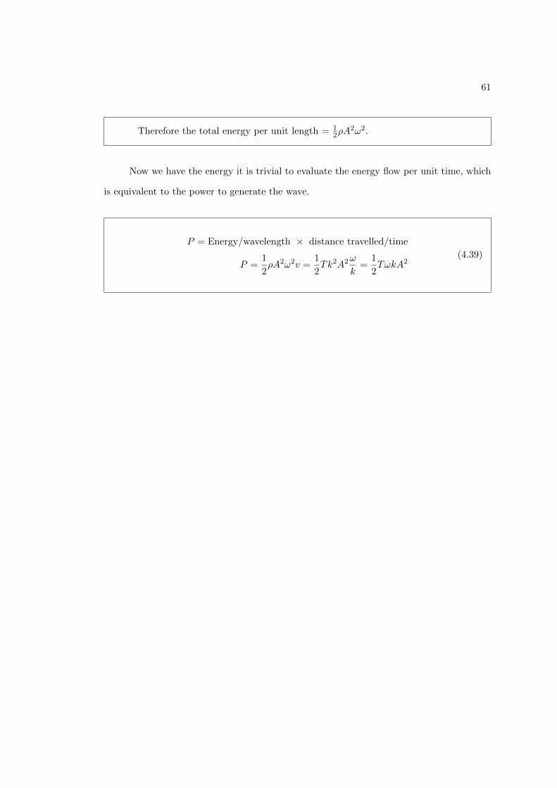
Now we have the energy it is trivial to evaluate the energy flow per unit time, which
is equivalent to the power to generate the wave.
P = Energy/wavelength ⇥ distance travelled/time
P =1
2⇢A
2
!
2
v =1
2Tk
2
A
2
!
k
=1
2T!kA
2
(4.39)