Wavelets

Chris Perkins, Tobin Fricke

Department of Electrical Engineering

University of California at Berkeley

December 1, 2000

1 Introduction

Convential time- and frequency- domain analysis have met with enormoussuccess in modern science and engineering. However, the scientific commu-nity is becoming increasingly aware that signals found in nature often exhibitcomplex, sometimes self-similar, even fractal characteristics. Wavelets are abroad class of new tools developed with the specific intent of being betterable to analyse these properties of real signals.

2 Background

2.1 The Fourier Transform

In the early 1800’s, Joseph Fourier discovered that nearly any function canbe expressed as a (possibly infinite) sum of sines and cosines, or, equivalently,complex exponentials (equivalent because of Euler’s identity: ejωt = j sinω+cosω, where j =

√−1).

A function f(t) is traditionally represented by defining its value for eachvalue of t in the domain of the function. In the terms of Linear Algebra, wecan say that the function is represented as a linear combination (a weightedsum) of delta functions. The discrete-time (Kronecker) delta function isdefined as follows:

δ(x) =

{

1 if x = 0,0 if x 6= 0.

(1)

Thus, for instance, we might define a simple sampled function imple-menting the mapping {0, 1, 2, 3} 7−→ {2, 7, 1, 8} as a linear combination of

1

delta functions:

f(x) = 2 · δ(x − 0) + 7 · δ(x− 1) + 1 · δ(x− 2) + 8 · δ(x− 3) + · · · (2)

The Fourier Transform allows us to find a new representation for thefunction, given by the coefficients of complex exponentials of integer multi-ples of some fundamental frequency. In other words, the Fourier Transformis simply a change of basis from the basis of delta functions {δ(x)} to thebasis of complex sinusoids {ejωn}. The basis of delta functions is usuallycalled the time (or space) domain, while the basis of complex exponentialsis called the frequency domain. The continuous-time transform to the fre-quency domain is:

f(ω) = F{f(t)} =

∫

∞

−∞

f(t)e−jωtdt (3)

To continue our example, we can use the Discrete Fourier Transform(not shown) to transform from the basis of delta functions to the basis ofcomplex sinusoids. The resulting linear combination implements the samefunction, just via a different representation:

f(x) =9

2· e0·jπn/2 +

1 + j

4· e1·jπn/2 + (−3) · e2·jπn/2 +

1− j

4· e3·jπn/2 (4)

The frequency domain has one serious shortcoming, however: it hasno time resolution. True, the frequency domain will tell us exactly whatfrequency components are present in a signal, but it tells us nothing aboutthe locality of those frequency components in time. For practical purposes,the Fourier Transform is only useful on steady-state, or “stationary” signals.

2.2 A Bit of Progress: The Windowed Fourier Transform

The basis functions of the frequency domain extend in time from negativeinfinity to positive infinity, oscillating forever in both directions. We say thatthese functions have “global extent”. In an attempt to add some locality oftime to the Fourier Transform, we can choose a new basis, one of sines andcosines modulated by the Gaussian.

We now have a transform that takes a one-dimensional function andreturns a two dimensional function: time on one axis, frequency on theother. This allows us to construct “spectrograms”, showing the relativefrequency content of a signal versus time.

2

While this can be extremely useful, it too has a serious shortcoming:the uncertainty principle. There is a fundamental trade-off between localityin the frequency domain and locality in the time domain. As we gain one,we lose the other. For instance, the frequency content localized at a singlepoint in a function is completely meaningless.

3 The Wavelet Transform

The Wavelet transform was inspired by the idea that we could vary thescale of the basis functions instead of their frequency: a subtle yet powerfulmodification. In the words of Amara Graps, “The fundamental idea behindwavelets is to analyze according to scale.” [1] Instead of representing afunction as a sum of weighted delta functions (as in the time domain), or asa sum of weighted sinusoids (as in the frequency domain), we represent thefunction as a sum of time-shifted (translated) and scaled (dilated) represen-tations of some arbitrary function, which as we shall see is called a wavelet.The power of this idea is that it examines the structure of information onall scales. The wavelet transform first compares the entire function to thewavelet, then compares smaller pieces of the function to the wavelet. Thisprocess is completed on successively smaller and smaller scales. This pro-cess forms a representation of the original function as a sum of wavelets ofvarious scales and positions in time, acheiving a balance between locality intime and locality in frequency/scale.

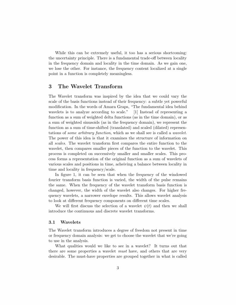
In figure 1, it can be seen that when the frequency of the windowedfourier transform basis function is varied, the width of the pulse remainsthe same. When the frequency of the wavelet transform basis function ischanged, however, the width of the wavelet also changes. For higher fre-quency wavelets, a narrower envelope results. This allows wavelet analysisto look at different frequency components on different time scales.

We will first discuss the selection of a wavelet ψ(t) and then we shallintroduce the continuous and discrete wavelet transforms.

3.1 Wavelets

The Wavelet transform introduces a degree of freedom not present in timeor frequency domain analysis: we get to choose the wavelet that we’re goingto use in the analysis.

What qualities would we like to see in a wavelet? It turns out thatthere are some properties a wavelet must have, and others that are verydesirable. The must-have properties are grouped together in what is called

3

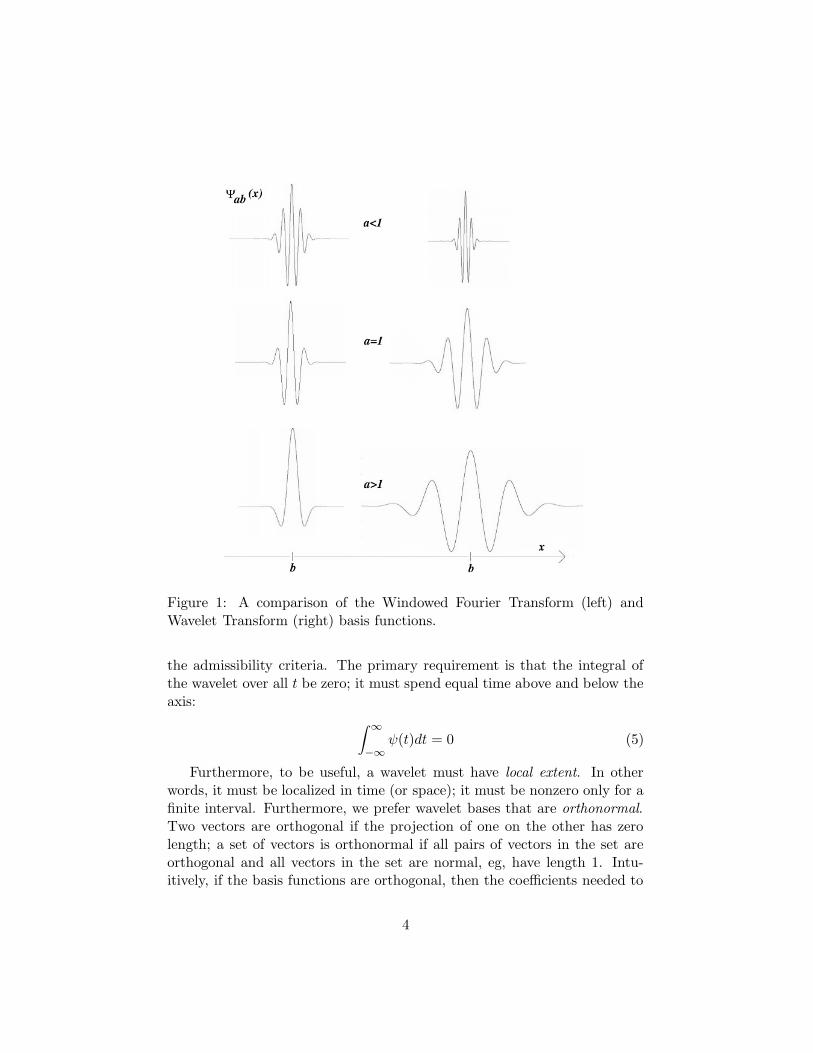
Figure 1: A comparison of the Windowed Fourier Transform (left) andWavelet Transform (right) basis functions.

the admissibility criteria. The primary requirement is that the integral ofthe wavelet over all t be zero; it must spend equal time above and below theaxis:

∫

∞

−∞

ψ(t)dt = 0 (5)

Furthermore, to be useful, a wavelet must have local extent. In otherwords, it must be localized in time (or space); it must be nonzero only for afinite interval. Furthermore, we prefer wavelet bases that are orthonormal.Two vectors are orthogonal if the projection of one on the other has zerolength; a set of vectors is orthonormal if all pairs of vectors in the set areorthogonal and all vectors in the set are normal, eg, have length 1. Intu-itively, if the basis functions are orthogonal, then the coefficients needed to

4

represent a linear combination will all represent independent information.With an orthonormal wavelet basis, it is possible that more information willbe compressed into fewer coefficients.

The first wavelet with these properties was discovered (or invented, de-pending on your weltanschauung) in 1910 by Alfred Haar [2], a Hungarianmathematician. The Haar wavelet is very simple; it just just a step function.Nonetheless it forms an orthonormal wavelet basis, and due to its simplic-ity and place in history it has also become the canonical example used inintroducing wavelets.

ψ(x) =

1 for 0 ≤ x < 1

2

−1 for 1

2≤ x < 1

0 otherwise(6)

The Haar wavelet is simple, but it is not ideal. It produces a basis setof predominantly flat functions, large numbers of which are required in lin-ear superposition to approximate a non-flat function. A better, smootherwavelet is needed. Yet, we would like to preserve the orthonormality of thewavelet basis. We need a mother wavelet that is localized in time and in fre-quency, is reasonably smooth, and ideally produces orthonormal translationsand dilations.

Only recently was such a wavelet found, by Ingrid Daubechies, now aprofessor at Princeton, in 1988 at AT&T Bell Laboratories. This function isnow known as the Daubechies Wavelet after its discoverer and has becomethe canonical “real” wavelet.

To understand the Daubechies wavelet, we must first introduce the scal-

ing equation. The scaling equation is a recursive expression that is usedto generate wavelets, so in some sense it is a “grandmother wavelet”. Inthe emphatic words of Gilbert Strang, “All good wavelet calculations use

recursion.” The scaling equation is given as [3]:

φj(t) =∑

ckφj−1(2x− k) (7)

To use the scaling equation to generate a mother wavelet, we must specifyseveral parameters. First, we must specify the the base case of the recursion,the function φ0(t). Second, we must specify coefficients {c0, c1, · · · , cN}. Forφ0 we use the box function, which is zero everywhere except the interval[0, 1]:

φ0(t) =

{

1 for 0 ≤ x ≤ 10 otherwise

(8)

5

The summation is over k: one term in the sum for each of the coefficients.It remains to specify what these “magic” coefficients are. The special valuesfound by Daubechies in 1998 are [3]:

{

c0 =1

4(1 +

√3), c1 =

1

4(3 +

√3), c2 =

1

4(3−

√3), c3 =

1

4(1−

√3)

}

(9)

Plugging these coefficients into the scaling equation and iterating, weget the Daubechies Wavlet (the Daubechies Wavlet is actually a class ofwavelets; this is the member that is generated from four coefficients.). Itshould not come as a suprise that the Daubechies Wavelet, generated in thisway, has fractal properties! Fractals arise in systems involving iteration orrecursion, and the generation of the Daubechies Wavelet very much followsthe recipe for generating fractals. In fact, the Daubechies Wavlet has anamazing property of self similarity: it actually contains a scaled down versionof itself! And this scaled down version in turn contains a scaled down version,ad infinitim. [4]

It is very easy to write a short computer program to demonstrate this,as we did. The source code is attached in the appendics.

-0.4

-0.2

0

0.2

0.4

0.6

0.8

1

1.2

1.4

0 0.5 1 1.5 2 2.5 3

"daub4"

-0.02

-0.01

0

0.01

0.02

0.03

0.04

0.05

0.06

0.07

2.3 2.4 2.5 2.6 2.7 2.8 2.9 3

"daub4_blowup"

Figure 2: T¯he Daubechies-4 wavelet. On the left, the complete Daubechies

wavelet is shown. The self-similarity of this wavelet is easily seen whenlooking more closely at the region between 2.4 and 3.0, as shown on theright.

When choosing a wavelet to use, it is advantageous to use a waveletthat resembles the signal to be analyzed. If such a wavelet is chosen, thesignal can be represented using significantly fewer coefficients than if a non-similar wavelet were used. In addition, choosing a wavelet that possessesself-similarity is also useful.

6

3.2 The Continuous Wavelet Transform

To use the Continuous Wavelet Transform (CWT), we first select a “motherwavelet” function, ψ(t). This could be the Haar wavelet, the Daubechieswavelet, or any other wavelet. We then form the vector projections of thefunction under analysis f(t) with dilations and translations of the motherwavelet:

W{x(t)} =

∫

∞

−∞

f(t)ψµν (t)dt ∀ν, µ (10)

where ψµν represents a specific dilation (µ) and translation (ν) of the

mother wavelet, ψ(t):

ψµν (t) =

√µψ

(

t− ν

µ

)

(11)

Although the continuous wavelet transform is very useful for theoreticalpurposes, in practice most signals are sampled, forming discrete data series.For these series we must use the Discrete Wavelet Transform.

3.3 The Discrete Wavelet Transform

The result of the Continuous Wavelet Transform of a one-dimensional signal(say, a time series for example) is a two-dimensional signal, with independentaxes of scale, and of time. Thus the CWT has introduced redundancy intothe representation of the signal. In the discrete case, the mother waveletis only scaled and dilated in discrete steps. “Dyadic” scalings are usuallychosen: one translation on the largest scale, two translations on a scale halfas large, four translations on a scale one quarter as large, etc. Thus thetranslation and dilation parameters in the wavelet transform become:

{

µ = 2−m

ν = n2−m (12)

For a data series of lengthN = N02M samples, the transform is evaluated

for the following scales and translations:

{

m = 1, 2, ...,Mn = 0, 1, ..., N02

m−1 − 1(13)

Notice that m chooses the scale (dilation) of the wavelet, and n choosesthe location (translation) of the wavelet. The value m = 1 corresponds tothe largest, most general scale, corresponding to the general shape of f(t)

7

over all t. Thus, we only have to evaluate one translation of the wavelet. Form = 2, we’ve halved the scale of our analysis, so it is necessary to evalue twotranslations. Hopefully this conveys an intuitive view of the dyadic scaling.

Using these relationships, we can form a set of orthogonal basis functionsfrom the mother wavelet ψ(t) and the relationships given above as:

ψmn (t) = 2m/2ψ(2mt− n) (14)

We then perform the wavelet transform as given in the continuous case,but with the integral reduced to a summation over a finite number ofterms [5].

4 Applications of Wavelet Analysis

Wavelet Analysis has found applications in numerous fields.Perhaps the most widespread use of Wavelets is in data compression in

general and in image compression in particular. The poster child of thisapplication cannot be anything other than the FBI fingerprint database,and the success of Wavelet analysis can also be seen in its adoption asthe compression technology to be used in the upcoming JPEG-2000 imagecompression standard. We will discuss image compression in some detail,and then summarize other applications of Wavelet technology.

4.1 Image Compression

The wavelet representation is extremely well suited for image compressionbecause it does not require the image to be broken down into sub-blocksfor processing. Furthermore, with Wavelet compression, an image can betransmitted as a data stream allowing progressive display of an image. Thefirst coefficients contain information about the image on the broadest scale;successive coefficients contain information about successively finer details.A user will have a good idea of what an image looks like after only a fewcoefficeints have been received, and may stop the transmission at any time.

In Wavelet-based image compression, the source image is first trans-formed to the Wavelet domain using the Discrete Wavelet Transform. Thesource is already of finite size, discretely sampled (into pixels), and quan-tized into a discrete set of colors (say, 256 levels of gray, red, green, or blue).Thus, the transformation into the wavelet domain is only a change-of-basis;no information is gained nor lost, and the resulting data takes up exactlythe same amount of space. We now quantize the data. To each wavelet

8

coefficient, we allocate a number of bits proportional to that coefficient’simportance in reconstruction. Low valued coefficients, by definition, con-tribute little to the reconstructed image. It is in this quantization step thatsome information is lost. Finally, the resulting quantized, Wavelet-domainrepresentation of the image is compressed using conventional, loss-less tech-niques, usually Huffman compression. The wavelet transform rearrangesthe information in an image so that the variations on differing scales aregrouped together. Usually the high-numbered coefficients, corresponding tovariation on the smallest scales, are very small: very often zero. Conven-tional compression is highly effective in compressing these regions of littlevariation. [6]

4.2 FBI Fingerprint Database

The American FBI has been collecting fingerprint cards since 1924 and inthis time has accumulated more than 200 million cards. The FBI digitizesthese cards for electronic storage, at a resolution of 500 dots per inch with256 levels of gray. A single fingerprint card results in about 10 megabytes ofdata; thus the entire collection would require 3000 terabytes, a truly hugeamount of data. Furthermore, about 40,000 new cards are now being addedper day. Add to this the needs to search for and retrieve cards from thedatabase on a daily basis, and it’s clear there’s a problem.

The FBI investigated the use of JPEG as a compressed image formatfor fingerprint data, but after some consultations with their friends at theUK Home Office Police Research Group, the conclusion was reached thatJPEG, and even custom JPEG variants, are unsuitable for compressionof fingerprints at ratios greater than about 10:1. The blocking artifactsproduced by JPEG at high levels of compression inhibited the interpretationof fingerprint data.

Eventually the FBI settled on a Wavelet based compression scheme de-veloped at Los Alamos National Laboratory, called Wavelet Scalar Quanti-zation. WSQ is a fairly typical wavelet image compression algorithm and hasproven to be enormously successful in storing fingerprint information. Withthe adoption of WSQ by the FBI as a standard data format for fingerprintinformation, it has become a de-facto standard worldwide as well. [7] [1] [8]

4.3 JPEG 2000

With the upcoming JPEG 2000 standard set to use wavelets as the founda-tion of its image compression mechanism, wavelets will soon enter the homes

9

of millions of people worldwide.JPEG 2000 will offer many improvements over the current generation of

JPEG compression. It will offer both lossy and lossless compression. It willfully exploit the desirable properties of the wavelet domain. Users will beable to view images at different resolutions corresponding to their needs andcapabilities. If only a preview of an image is needed, the wavelet datastreamcan be terminated very early, but when a higher quality image is needed,more of the wavelet datastream can be decoded. [9]

4.4 Audio Compression

It will be interesting to see what fields Wavelet Analysis shall next infiltrate.MP3, a Fourier-based audio compression technology, coupled with relativelywide access to high-bandwidth internet connectivity, is poised to cause acomplete reorganization of the music industry as well as American copyrightlaw. Could wavelets be applied to audio for even greater compression or lessdegradation in quality?

Unfortunately one of the qualities that makes Wavelets so incredibly wellsuited for image compression is a drawback when audio compression is con-sidered. When we view images, we take in the entire image at once. Firstwe perceive general features of the image, and then we look at the finerdetails. The wavelet transform allows images to be displayed progressivelyin a way very suited to the human visual system. The more coefficients arereceived, the higher the quality of the resulting image. Audio, on the otherhand, the human brain processes linearly. When listening to a song, we donot comprehend the entire song in its entirety all at once; we comprehendthe song moment-by-moment, and how it develops over time is important.Thus the wavelet approach – where the “general idea” of the song wouldbe available first, followed by the details, would not be appropriate for pro-gressive, real-time transmission of audio, for example over the internet. Wewould have to wait for a sufficient number of coefficentsto be received beforestarting playback.

This practical detail aside, we speculate that audio is well suited towavelet compression. Music traditionally exhibits a high degree of self-similarity, and, moreover, self-similarity on a multitude of scales. Thesefeatures are exactly those that the wavelet transform exploits, so it wouldbe interesting to examine the application of wavelet analysis to audio inanother project at another time.

10

4.5 Other Applications

Wavelet analysis has permeated nearly every region of modern science. Inany field where data needs to be analyzed, wavelet analysis is often ableto give insights that more traditional data analysis techniques cannot pro-vide. In the field of astronomy and cosmology, wavelet analysis is usefulin analyzing stellar and solar data and has provided information about thesun and other stellar processes that methods such as Fourier analysis havenot been able to provide. Wavelet analysis is also used in these fields tocompress telescopic image data (such as that from the Hubble Space Tele-scope). Wavelet analysis is also useful in analyzing seismic data. Algorithmsare needed to determine when an earthquake begins and to study variousproperties of the motion. Wavelet analysis is a natural candidate to analyzesuch data. Wavelet analysis has also provided new insights in the studyof turbulence. Wavelets are also used extensively in computer graphics toperform edge-detection, texture analysis, and denoising of image data. [10]

Wavelet analysis has also been incorporated into so-called “Fractal Mod-ulation”, a new scheme for modulating data for transmission over a wire.Officially known as DWMT, or Discrete Wavelet Multi-Tone Modulation,and developed by Aware, Inc., this technology is one of several being inves-tigated for use in next-generation Digital Subscriber Line technology. DigitalSubscriber Line (DSL) is a means of sending and receiving high-speed dig-ital data to and from residences over the same copper wires that are usedfor regular telephone service – indeed, the system operates simultaneously

with regular telephone service. With greater and greater needs for high-bandwidth internet connectivity at home, being able to squeeze every lastbit per second out of existing infrastructure is also increasing in importance,and Wavelets may have a significant influence in this field. [11]

One reason that wavelet analysis is so useful in such a wide range ofphysical applications is that physical signals usually have different frequencycomponents on different spatial scales. There are usually very short, highfrequency signals mixed with longer, low frequency signals. Wavelet analysislends itself perfectly to such signals because of its ability to look at differentspatial regions using different scales.

11

5 An Experiment In Image Compression

5.1 Motivation

There is a vast amount of literature available on the subject of wavelets, how-ever most consists of mathematical text with little information on practicalapplication of wavelet technology. Outrageous claims are made regardingthe capabilities of wavelet-based techniques, yet it is difficult to find ele-gant, compelling examples of the success of wavelet analysis.

We set out to verify whether or not wavelets could do everything theypromised, specifically in the area of image compression.

5.2 Procedure

We first selected a test image. We could not resist the temptation to usethe professor’s portrait as it appears on his webpage, instead of a more tra-ditional IEEE test image of some sort. We first converted this image fromJPEG format to the much-simpler Portable Greymap (PGM) image file for-mat, which is essentially a list of pixel values in plain, human-readable text.To do this we used a free software program developed at UC Berkeley’seXperimental Computing Facility (the XCF), the GNU Image Manipula-tion Program (more affectionately known as The GIMP). The next step wasto implement the two-dimensional Discrete Wavelet Transform. We werepleased to find an implementation available in the popular reference, Nu-

merical Recipes In C [12]. We wrote a C program that reads in the PGMformat image of the professor into a row-major linear array. Next, we usethe Numerical Recipes routines to compute the discrete wavelet transformalong two dimensions. Now, we make a copy of the resulting array, and weuse the C standard library routine qsort() to sort it. This allows us to findthe value of the nth highest coefficient. We then set to zero some percent-age of the lowest-valued coefficients. Finally, we take the inverse discretewavelet transform resulting in a regular image once again. The programoutputs the pixel values of the image to a file, which we then load in Matlaband compare to the original. To summarize, the procedure is as follows:

1. Load the source image data from a file into an array

2. Compute the Discrete Wavelet Transform of the data

3. Remove (set to zero) all coefficients whose value is below a threshold.(This is the compression step.)

12

4. Reconstruct the image by computing the Inverse Discrete WaveletTransform

5. Compare the resulting reconstruction of the compressed image to theoriginal image

The C source code to this software is listed in the appendix.

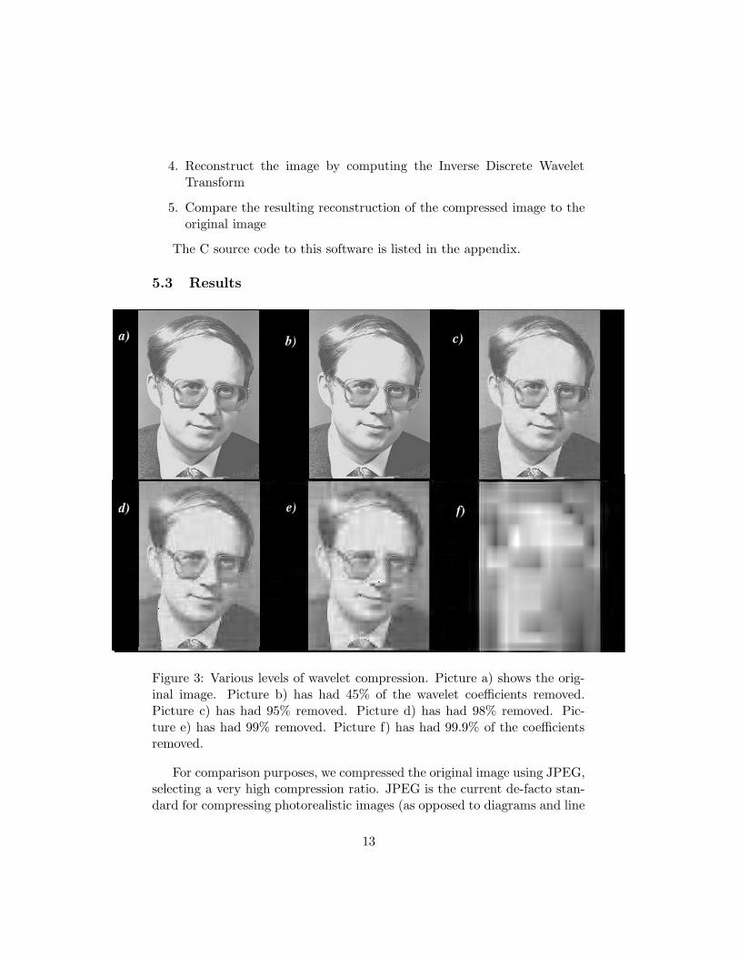
5.3 Results

Figure 3: Various levels of wavelet compression. Picture a) shows the orig-inal image. Picture b) has had 45% of the wavelet coefficients removed.Picture c) has had 95% removed. Picture d) has had 98% removed. Pic-ture e) has had 99% removed. Picture f) has had 99.9% of the coefficientsremoved.

For comparison purposes, we compressed the original image using JPEG,selecting a very high compression ratio. JPEG is the current de-facto stan-dard for compressing photorealistic images (as opposed to diagrams and line

13

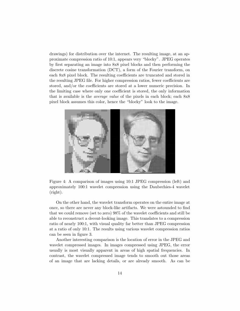
drawings) for distribution over the internet. The resulting image, at an ap-proximate compression ratio of 10:1, appears very “blocky”. JPEG operatesby first separating an image into 8x8 pixel blocks and then performing thediscrete cosine transformation (DCT), a form of the Fourier transform, oneach 8x8 pixel block. The resulting coefficients are truncated and stored inthe resulting JPEG file. For higher compression ratios, fewer coefficients arestored, and/or the coefficients are stored at a lower numeric precision. Inthe limiting case where only one coefficient is stored, the only informationthat is available is the average value of the pixels in each block; each 8x8pixel block assumes this color, hence the “blocky” look to the image.

Figure 4: A comparison of images using 10:1 JPEG compression (left) andapproximately 100:1 wavelet compression using the Daubechies-4 wavelet(right).

On the other hand, the wavelet transform operates on the entire image atonce, so there are never any block-like artifacts. We were astounded to findthat we could remove (set to zero) 98% of the wavelet coefficients and still beable to reconstruct a decent-looking image. This translates to a compressionratio of nearly 100:1, with visual quality far better than JPEG compressionat a ratio of only 10:1. The results using various wavelet compression ratioscan be seen in figure 3.

Another interesting comparison is the location of error in the JPEG andwavelet compressed images. In images compressed using JPEG, the errorusually is most visually apparent in areas of high spatial frequencies. Incontrast, the wavelet compressed image tends to smooth out those areasof an image that are lacking details, or are already smooth. As can be

14

seen in figure 3, even with a compression ratio of approximately 100:1, highresolution regions can still be seen, such as the areas around the glasses,mouth, necktie, and hair, while lower frequency regions, such as the suitand other facial regions have been smoothed out. This mix of sharp andsmooth regions demonstrates how the wavelet transform is able to analyzedifferent spatial regions using different scales.

0

1e+06

2e+06

3e+06

4e+06

5e+06

6e+06

7e+06

8e+06

9e+06

1e+07

0 0.1 0.2 0.3 0.4 0.5 0.6 0.7 0.8 0.9 1

"error"

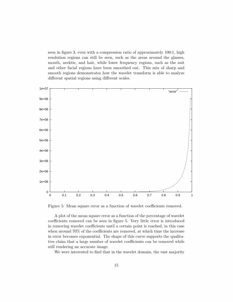
Figure 5: Mean square error as a function of wavelet coefficients removed.

A plot of the mean square error as a function of the percentage of waveletcoefficients removed can be seen in figure 5. Very little error is introducedin removing wavelet coefficients until a certain point is reached, in this casewhen around 70% of the coefficients are removed, at which time the increasein error becomes exponential. The shape of this curve supports the qualita-tive claim that a large number of wavelet coefficients can be removed whilestill rendering an accurate image.

We were interested to find that in the wavelet domain, the vast majority

15

of coefficients are very small. Indeed, the highest coefficient in our test caseexceeded the lowest coefficient by five orders of magnitude!

16

6 Conclusion

Wavelet analysis is able to transform a time- or space- domain signal toa new basis, the wavelet domain, that takes advantage of the character ofreal signals. Most real-life data cannot be concisely modeled using onlytime series or fourier series, but the wavelet transform has been remarkablysuccessful in exploiting the fractal characteristics of these signals. Becauseof this, wavelet-based compression is phenominally effective, and as timegoes on will become more and more pervasive. Furthermore, knowledgegained through wavelet analysis in diverse fields may lead to significant newknowledge of the world. Wavelet theory is maturing rapidly and is becomingmore and more widely known. This will likely lead to even more applicationsof wavelet analysis in years to come.

References

[1] Amara Graps. “An Introduction to Wavelets”. IEEE Computational

Science and Engineering, vol. 2, num. 2 (Summer 1995).

[2] Gilbert Strang. “Wavelets”. American Scientist, 82 (1994) 250-255.

[3] Gilbert Strang. “Wavelets and Dilation Equations: A Brief Introduc-tion”. Siam Review, 31 (1989) 613-627.

[4] Ingrid Daubechies. “Ten Lectures On Wavelets”. Society for Industrialand Applied Mathematics, (1992).

[5] Gregory W. Wornell. “Signal Processing With Fractals: A Wavelet-

Based Approach”. Prentice Hall, (1996).

[6] Subhasis Saha. “Image Compression -from DCT to Wavelets”. ACM Crossroads.http://www.acm.org/crossroads/xrds6-3/sahaimgcoding.html.

[7] Chris Brislawn. The FBI Fingerprint Image Compression Standard.http://www.c3.lanl.gov/~brislawn/FBI/FBI.html.

[8] Chris Brislawn. Fingerprints Go Digital, vol. 42 no. 11 (Nov. 1995)1278-1283.

[9] Michael J. Gormish. “JPEG 2000: Worth the Wait?”.

17

[10] J.C. van den Berg. “Wavelets in Physics”. Cambridge University Press,(1999).

[11] Stuart D. Sandberg and Michael A. Tzannes. “Overlapped DiscreteMultitone Modulations for High Speed Copper Wire Communications”.Aware, Inc., (1995).

[12] William H. Press et al. “Numerical Recipes in C”. Cambridge Univer-sity Press, (1992).

18