1

Wavelet Transform Theory

Prof. Mark FowlerDepartment of Electrical Engineering

State University of New York at Binghamton

2

What is a Wavelet Transform?

• Decomposition of a signal into constituent parts• Note that there are many ways to do this. Some are:

– Fourier series: harmonic sinusoids; single integer index– Fourier transform (FT): nonharmonic sinusoids; single real index– Walsh decomposition: “harmonic” square waves; single integer index– Karhunen-Loeve decomp: eigenfunctions of covariance; single real index– Short-Time FT (STFT): windowed, nonharmonic sinusoids; double index

• provides time-frequency viewpoint– Wavelet Transform: time-compacted waves; double index

• Wavelet transform also provides time-frequency view– Decomposes signal in terms of duration-limited, band-pass components

• high-frequency components are short-duration, wide-band• low-frequency components are longer-duration, narrow-band

– Can provide combo of good time-frequency localization and orthogonality• the STFT can’t do this

– More precisely, wavelets give time-scale viewpoint• this is connected to the multi-resolution viewpoint of wavelets

3

General Characteristics of Wavelet Systems

• Signal decomposition: build signals from “building blocks”, where the building blocks (i.e. basis functions) are doubly indexed.

• The components of the decomposition (i.e. the basis functions) are localized in time-frequency

– ON can be achieved w/o sacrificing t-f localization • The coefficients of the decomposition can be computed efficiently (e.g.,

using O(N) operations).

Specific Characteristics of Wavelet Systems• Basis functions are generated from a single wavelet or scaling function

by scaling and translation• Exhibit multiresolution characteristics: dilating the scaling functions

provides a higher resolution space that includes the original• Lower resolution coefficients can be computed from higher resolution

coefficients through a filter bank structure

4

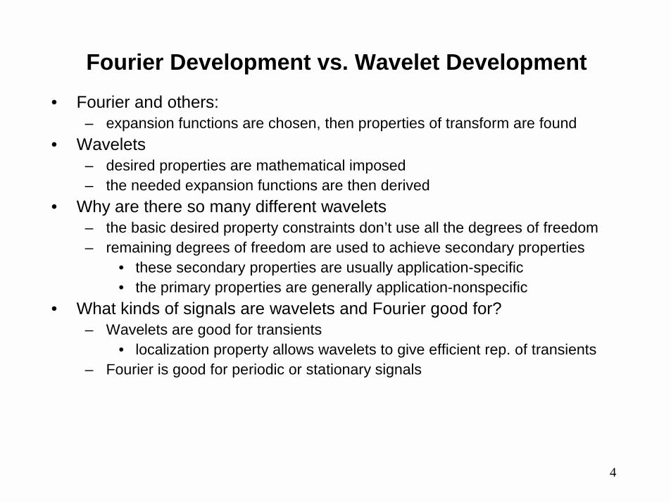
Fourier Development vs. Wavelet Development• Fourier and others:

– expansion functions are chosen, then properties of transform are found• Wavelets

– desired properties are mathematical imposed– the needed expansion functions are then derived

• Why are there so many different wavelets– the basic desired property constraints don’t use all the degrees of freedom– remaining degrees of freedom are used to achieve secondary properties

• these secondary properties are usually application-specific• the primary properties are generally application-nonspecific

• What kinds of signals are wavelets and Fourier good for?– Wavelets are good for transients

• localization property allows wavelets to give efficient rep. of transients– Fourier is good for periodic or stationary signals

5

Why are Wavelets Effective?• Provide unconditional basis for large signal class

– wavelet coefficients drop-off rapidly– thus, good for compression, denoising, detection/recognition– goal of any expansion is

• have the coefficients provide more info about signal than time-domain• have most of the coefficients be very small (sparse representation)

– FT is not sparse for transients• Accurate local description and separation of signal characteristics

– Fourier puts localization info in the phase in a complicated way– STFT can’t give localization and orthogonality

• Wavelets can be adjusted or adapted to application– remaining degrees of freedom are used to achieve goals

• Computation of wavelet coefficient is well-suited to computer– no derivatives of integrals needed– turns out to be a digital filter bank

6

Multiresolution Viewpoint

7

Multiresolution Approach• Stems from image processing field

– consider finer and finer approximations to an image• Define a nested set of signal spaces

• We build these spaces as follows:• Let be the space spanned by the integer translations of a

fundamental signal φ(t), called the scaling function:

that is, if f(t) is in then it can be represented by:

• So far we can use just about any function φ(t), but we’ll see that to get the nesting only certain scaling functions can be used.

221012 LVVVVV ⊂⊂⊂⊂⊂⊂⊂ −− !!

0V

0V

∑ −=k

k ktatf )()( φ

8

Multiresolution Analysis (MRA) Equation• Now that we have how do we make the others and ensure that they

are nested?• If we let be the space spanned by integer translates of φ(2t) we get

the desired property that is indeed a space of functions having higher resolution.

• Now how do we get the nesting?• We need that any function in also be in ; in particular we need

that the scaling function (which is in ) be in , which the requires that

where the expansion coefficient is • This is the requirement on the scaling function to ensure nesting: it

must satisfy this equation– called the multiresolution analysis (MRA) equation– this is like a differential equation that the scaling function is the solution to

0V

1V1V

0V 1V

0V 1V

∑ −=n

ntnht )2(2)()( φφ

2)(nh

9

The h(n) Specify the Scaling Function• Thus, the coefficients h(n) determine the scaling function

– for a given set of h(n), φ(t)• may or may not exist• may or may not be unique

• Want to find conditions on h(n) for φ(t) to exist and be unique, and also:– to be orthogonal (because that leads to an ON wavelet expansion)– to give wavelets that have desirable properties

h(n)

n

φφφφ(t)

tMRA Equation

h(n) must satisfy

conditions

h(n) must satisfy

conditions

10

Whence the Wavelets?• The spaces Vj represent increasingly higher resolution spaces• To go from Vj to higher resolution Vj+1 requires the addition of “details”

– These details are the part of Vj+1 not able to be represented in Vj

– This can be captured through the “orthogonal complement of Vj w.r.t Vj+1

• Call this orthogonal complement space Wj– all functions in Wj are orthogonal to all functions in Vj

– That is:

• Consider that V0 is the lowest resolution of interest• How do we characterize the space W0 ?

– we need to find an ON basis for W0, say where the basis functions arise from translating a single function (we’ll worry about the scaling part later):

Z∈∀=>=< ∫ lkjdttttt ljkjljkj ,,0)()()(),( ,,,, ψφψφ

{ })(,0 tkψ

)()(,0 kttk −=ψψ

11

Finding the Wavelets• The wavelets are the basis functions for the Wj spaces

– thus, they lie in Vj+1

• In particular, the function lies in the space V1 so it can be expanded as

• This is a fundamental result linking the scaling function and the wavelet– the h1(n) specify the wavelet, via the specified scaling function

)(tψ

∑ ∈−=n

nntnht Z),2(2)()( 1 φψ

h1(n)

n

ψψψψ(t)

t

h1(n) must satisfy

conditions

h1(n) must satisfy

conditions

Wavelet Equation

(WE)

12

Wavelet-Scaling Function Connection• There is a fundamental connection between the scaling function and its

coefficients h(n) , the wavelet function and its coefficients h1(n):

h1(n)

n

ψψψψ(t)

t

h(n)

n

φφφφ(t)

t

How are h1(n) and h(n) related?

Wavelet Equation

(WE)

MR Equation

(MRE)

13

Relationship Between h1(n) and h(n)

• We state here the conditions for the important special case of– finite number N of nonzero h(n)– ON within V0:– ON between V0 and W0 :

• Given the h(n) that define the desired scaling function, then the h1(n) that define the wavelet function are given by

• Much of wavelet theory addresses the origin, characteristics, and ramifications of this relationship between h1(n) and h(n)

– requirements on h(n) and h1(n) to achieve ON expansions– how the MRE and WE lead to a filter bank structure– requirements on h(n) and h1(n) to achieve other desired properties– extensions beyond the ON case

∫ =− )()()( kdtktt δφφ

∫ =− )()()( kdtktt δφψ

)1()1()(1 nNhnh n −−−=

14

The Resulting Expansions• Let f(t) be in L2(R)• There are three ways of interest that we can expand f(t)

1 We can give an limited resolution approximation to f(t) via

– increasing j gives a better (i.e., higher resolution) approximation

– this is in general not the most useful expansion

∑ −=k

jjkj ktatf )2(2)( 2/ φ

221012 LVVVVV ⊂⊂⊂⊂⊂⊂⊂ −− !!

15

The Resulting Expansions (cont.)

2 A low-resolution approximation plus its wavelet details

– Choosing j0 sets the level of the coarse approximation

– This is most useful in practice: j0 is usually chosen according to application• Also in practice, the upper value of j is chosen to be finite

∑∑∑∞

=

−+−=0

000

)2(2)()2(2)()( 2/2/

jj

jjj

kk

jjj ktkdktkctf ψφ

!⊕⊕⊕⊕= ++ 212

0000 jjjj WWWVL

Low-Resolution Approximation

Wavelet Details

16

The Resulting Expansions (cont.)

3 Only the wavelet details

– Choosing j0=-∞ eliminates the coarse approximation leaving only details

– This is most similar to the “true” wavelet decomposition as it was originally developed

– This is not that useful in practice: j0 is usually chosen to be finite according to application

∑∑∞

−∞=

−=j

jjj

k

ktkdtf )2(2)()( 2/ ψ

!! ⊕⊕⊕⊕⊕⊕= −− 210122 WWWWWL

17

The Expansion Coefficients cj0(k) and dj(k)

• We consider here only the simple, but important, case of ON expansion– i.e., the φ’s are ON, the ψ’s are ON, and the φ’s are ON to the ψ’s

• Then we can use standard ON expansion theory:

• We will see how to compute these without resorting to computing inner products

– we will use the coefficients h1(n) and h(n) instead of the wavelet and scaling function, respectively

– we look at a relationship between the expansion coefficients at one level and those at the next level of resolution

dtttfttfkc kjkjj ∫== )()()(),()( ,, 000ϕϕ

dtttfttfkd kjkjj ∫== )()()(),()( ,, ψψ

18

Summary of Multiresolution View• Nested Resolution spaces:

• Wavelet Spaces provide orthogonal complement between resolutions

• Wavelet Series Expansion of a continuous-time signal f(t):

• MR equation (MRE) provides link between the scaling functions atsuccessive levels of resolution:

• Wavelet equation (WE) provides link between a resolution level and its complement

∑∑∑∞

=

−+−=0

000

)2(2)()2(2)()( 2/2/

jj

jjj

kk

jjj ktkdktkctf ψφ

221012 LVVVVV ⊂⊂⊂⊂⊂⊂⊂ −− !!

!⊕⊕⊕⊕= ++ 212

0000 jjjj WWWVL

Z∈−=∑ nntnhtn

,)2(2)()( φφ

∑ ∈−=n

nntnht Z),2(2)()( 1 φψ

19

Summary of Multiresolution View (cont.)• There is a fundamental connection between the scaling function and its

coefficients h(n) , the wavelet function and its coefficients h1(n):

h1(n)

n

ψψψψ(t)

t

h(n)

n

φφφφ(t)

tMR Equation

(MRE)

How are h1(n) and h(n) related?

Wavelet Equation

(WE)

20

Filter Banks and DWT

21

Generalizing the MRE and WE• Here again are the MRE and the WE:

• We get:

∑ −=n

ntnht )2(2)()( φφ ∑ −=n

ntnht )2(2)()( 1 φψ

scale & translate: replace ktt j −→ 2

∑ −−=− +

m

jj mtkmhkt )2(2)2()2( 1φφ

Connects Vj to Vj+1

MRE

∑ −−=− +

m

jj mtkmhkt )2(2)2()2( 11 φψ

Connects Wj to Vj+1

WE

22

Linking Expansion Coefficients Between Scales • Start with the Generalized MRA and WE:

∑ −−=− +

m

jj mtkmhkt )2(2)2()2( 1φφ ∑ −−=− +

m

jj mtkmhkt )2(2)2()2( 11 φψ

)(),()( , ttfkc kjj ϕ= )(),()( , ttfkd kjj ψ=

)()2()( 1 mckmhkc jm

j +∑ −=

∑ −−= ++

m

jjj mttfkmhkc )2(2),()2()( 12/)1( ϕ

)()2()( 11 mckmhkd jm

j +∑ −=

∑ −−= ++

m

jjj mttfkmhkd )2(2),()2()( 12/)1(

1 ϕ

)(1 mc j+

23

Convolution-Decimation Structure

)()2()( 10 mckmhkc jm

j +∑ −= )()2()( 11 mckmhkd jm

j +∑ −=

New Notation For Convenience: h(n) →→→→h0(n)

)()(

)()()(

10

010

mcnmh

nhncny

jm

j

+

+

∑ −=

−∗=

)()(

)()()(

11

111

mcnmh

nhncny

jm

j

+

+

∑ −=

−∗=Convolution

Decimation

k=0 1 2 3 4

n=0 1 2 3 4 5 6 7 8 9

n = 2k =0 2 4 6 8

24

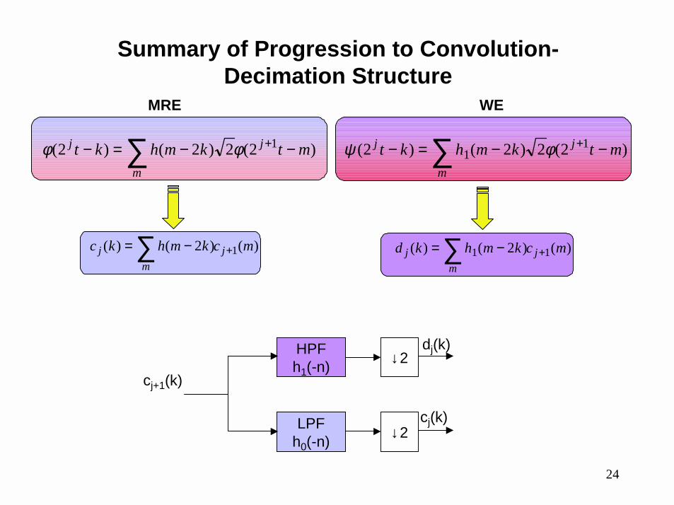
Summary of Progression to Convolution-Decimation Structure

∑ −−=− +

m

jj mtkmhkt )2(2)2()2( 1φφ

MRE

∑ −−=− +

m

jj mtkmhkt )2(2)2()2( 11 φψ

WE

)()2()( 1 mckmhkc jm

j +∑ −= )()2()( 11 mckmhkd jm

j +∑ −=

LPF h0(-n)

HPF h1(-n)

cj+1(k)

cj(k)

dj(k)↓2

↓2

25

Computing The Expansion Coefficients• The above structure can be cascaded:

– given the scaling function coefficients at a specified level all the lower resolution c’s and d’s can be computed using the filter structure

LPF h0(-n)

HPF h1(-n)

cj+1(k)

cj(k)

dj(k)↓2

↓2

LPF h0(-n)

HPF h1(-n)

cj-1(k)

↓2

↓2

LPF h0(-n)

HPF h1(-n)

cj-2(k)

↓2

↓2

dj-1(k)

dj-2(k)

Vj+1

Vj

Vj-1

Vj-2

Wj

Wj-1

Wj-2

26

Filter Bank Generation of the Spaces

LPF h0(-n)

HPF h1(-n) ↓2

↓2

LPF h0(-n)

HPF h1(-n) ↓2

↓2

LPF h0(-n)

HPF h1(-n) ↓2

↓2

Vj+1

Vj

Vj-1

Vj-2

Wj

Wj-1

Wj-2

WjWj-1Wj-2Vj-2

Vj+1

ππ/2π/4π/8

27

Time

Freq

DISCRETE FOURIER TRANSFORM

28

Time

Freq

WAVELET TRANSFORM

29

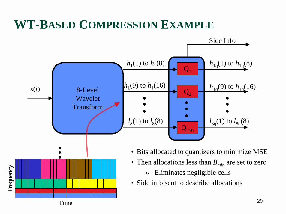
Q256

Q1

Q28-LevelWavelet

Transform

h1(1) to h1(8)

h1(9) to h1(16)

l8(1) to l8(8)

h1q(1) to h1q(8)

h1q(9) to h1q(16)

l8q(1) to l8q(8)

Side Info

s(t)

• Bits allocated to quantizers to minimize MSE• Then allocations less than Bmin are set to zero

» Eliminates negligible cells• Side info sent to describe allocations

WT-BASED COMPRESSION EXAMPLE

Time

Freq

uenc

y