Embed Size (px)
Citation preview
Wavelet Galerkin FEM
for
Operator Equations with Stochastic Data
Ch. Schwab
Seminar fur Angewandte Mathematik
ETH Zurich, Switzerland
Joint with Tobias von Petersdorff, UM College ParkCEMRACS06 July+August 2006, Luminy, France.
IHP Network “Breaking Complexity” EC contract number HPRN-CT-2002-00286Swiss Federal Office for Science and Education grant No. BBW 02.0418.

Numerical models in engineering can be solved with high accuracy
if input data are known exactly.
Often, however,
input data are not known exactly
and
accurate numerical solutions are of limited use.
•Mathematical description of uncertainty in input data and solution?
• How to propagate data uncertainty through an engineering FEM simulation?
• How to process statistical information in FEM?
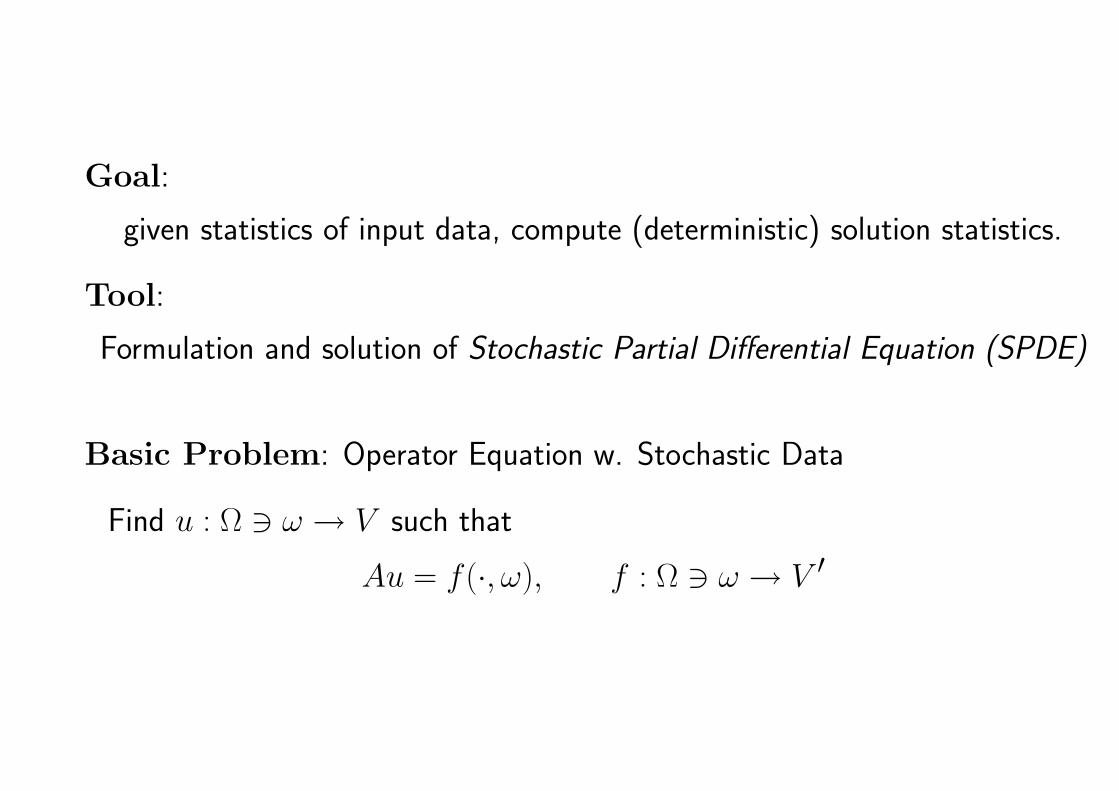
Goal:
given statistics of input data, compute (deterministic) solution statistics.
Tool:
Formulation and solution of Stochastic Partial Differential Equation (SPDE)
Basic Problem: Operator Equation w. Stochastic Data
Find u : Ω 3 ω → V such that
Au = f (·, ω), f : Ω 3 ω → V ′

literature
References
Perturbation Methods; “First Order Second Moment” (FOSM)
J. B. Keller (1964)
M. Kleiber, T.D. Hien (1992)
CS and R.A. Todor (2003)
Stochastic Galerkin; Wiener Polynomial Chaos (Karhunen-Loeve)
R. G. Ghanem, P. D. Spanos (1991)
I. Babuska , J.T. Oden et al. (2001)
G. E. Karniadakis, D. Xiu (2002)
Matthies and Keese (2005)

Outline
1 Random fields, statistics
2 Stochastic boundary value problem (sBVP)
3 Stochastic Operator Equations
4 Example: Stochastic boundary integral equation (sPDE)
5 Sparse Monte Carlo FEM
6 Sparse Tensor Product FEM
7 Conclusions
8 Application: 2nd Moment Analysis in Random Domains

random fields
Random fields, statistics
D ⊂ Rd bounded domain, Γ = ∂D = Γ0 ∪ Γ1 Lipschitz,
(Ω,Σ, P ) probability space
Random fields on Γ, D:
X separable Hilbert space. u(x, ω) random field iff
u ∈ L0(Ω, X) := u(x, ω) : Ω→ X| Ω 3 ω → ‖u(·, ω)‖X is P -measurable
A random field u : Ω→ X is in L1(Ω, X) if ω 7→ ‖u(ω)‖X is integrable so that
‖u‖L1(Ω,X) :=Ω
‖u(ω)‖X dP (ω) <∞
In this case the Bochner integral
Eu :=Ω
u(ω)dP (ω) ∈ X
exists and we have
‖Eu‖X ≤ ‖u‖L1(Ω,X) . (1)
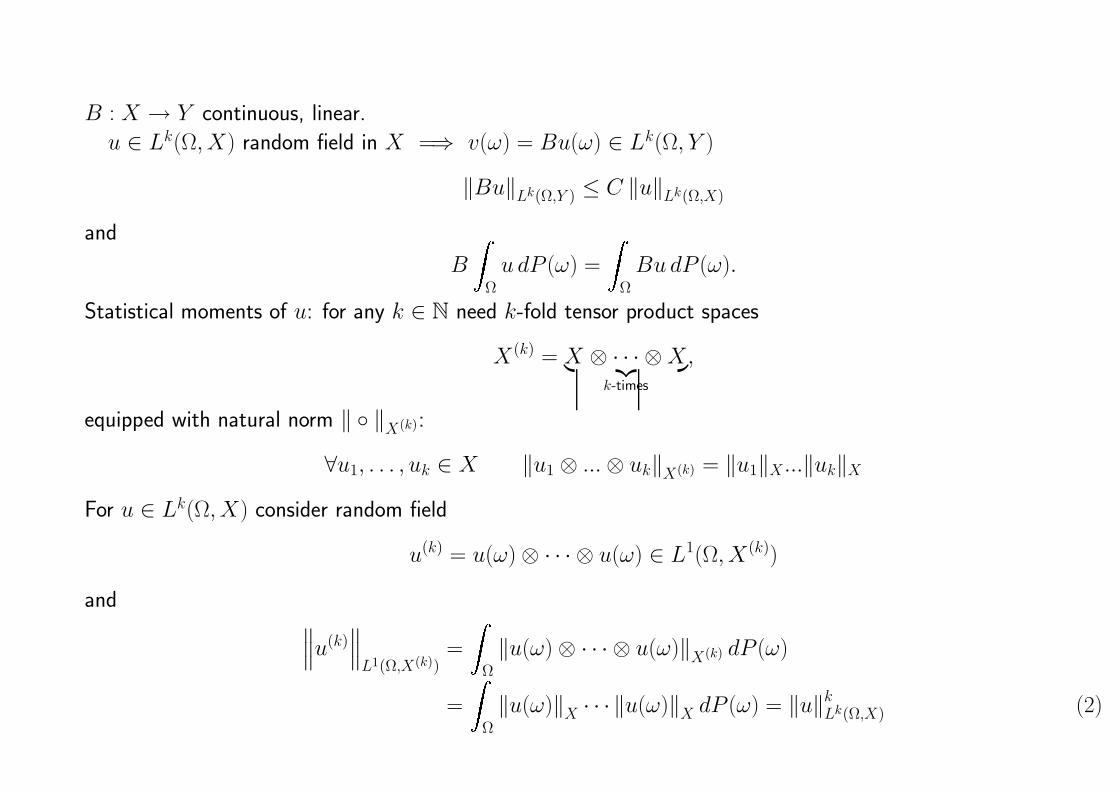
B : X → Y continuous, linear.
u ∈ Lk(Ω, X) random field in X =⇒ v(ω) = Bu(ω) ∈ Lk(Ω, Y )
‖Bu‖Lk(Ω,Y ) ≤ C ‖u‖Lk(Ω,X)
and
BΩ
u dP (ω) =Ω
BudP (ω).
Statistical moments of u: for any k ∈ N need k-fold tensor product spaces
X(k) = X ⊗ · · · ⊗X︸ ︷︷ ︸k-times
,
equipped with natural norm ‖ ‖X(k):
∀u1, . . . , uk ∈ X ‖u1 ⊗ ...⊗ uk‖X(k) = ‖u1‖X ...‖uk‖XFor u ∈ Lk(Ω, X) consider random field
u(k) = u(ω)⊗ · · · ⊗ u(ω) ∈ L1(Ω, X(k))
and∥∥∥u(k)
∥∥∥L1(Ω,X(k))
=Ω
‖u(ω)⊗ · · · ⊗ u(ω)‖X(k) dP (ω)
=Ω
‖u(ω)‖X · · · ‖u(ω)‖X dP (ω) = ‖u‖kLk(Ω,X) (2)

Define k-th moment (k-point correlation function) Mku as expectation of u⊗ · · · ⊗ u:
Definition 0
For u ∈ Lk(Ω, X) for some integer k ≥ 1, the k-th moment of u(ω) is defined by
Mku = E[u⊗ ...⊗ u︸ ︷︷ ︸k−times
] =
ω∈Ω
u(ω)⊗ ...⊗ u(ω)︸ ︷︷ ︸k−times
dP (ω) ∈ X (k) (3)
Application: Covariance of u ∈ L2(Ω, V ), V separable and reflexive.
Cov[u] = E [(u− Eu)⊗ (u− Eu)] ∈ V ⊗ V
If u “sufficiently regular”:
Covariance:
Cov[u](x, x′) =Ω
(u(x, ω)− Eu(x))(u(x′, ω)− Eu(x′))dP (ω), x, x′ ∈ D.
k-th Moment (k-point correlation function): if u ∈ Lk(Ω, V ), thenM(k)u = E[u⊗ ...⊗ u] ∈ V (k) := V ⊗ ...⊗ V :
M(k)u(x1, ..., xk) :=Ω
u(x1, ω)⊗ ...⊗ u(xk, ω) dP (ω)

stochastic operator equation
Stochastic Operator Equation
Given A : V → V ′ linear, bounded, f ∈ L1(Ω, V ′), find u ∈ L1(Ω, V ):
Au = f
Assume ex. α > 0 and T : V → V ′ compact such that
∀v ∈ V :⟨(A + T ) v, v
⟩≥ α ‖v‖2
V (4)
and
kerA = 0 (5)
Proposition 1
Assume (4) and (5). Then for every f ∈ L0(Ω, V ′) exists a unique u ∈ L0(Ω, V ) solution of Au = f .

moments, statistics
Statistics
Mean Field: if u ∈ L1(Ω, V )
Eu ∈ V :
Eu(x) :=Ω
u(x, ω) dP (ω)
Covariance: if u ∈ L2(Ω, V )
C[u] ∈ V ⊗ V :
C[u](x, y) :=Ω
(u(x, ω)−Eu(x))(u(y, ω)− Eu(y)) dP (ω)
Variance: (Varu)(x) = E[u2](x)− (E[u](x))2 = (M(2)[u])(x, x)− (E[u](x))2
kth Moment: if u ∈ Lk(Ω, V )
M(k)u ∈ V (k) := V ⊗ ...⊗ V :
M(k)u(x1, ..., xk) :=Ω
u(x1, ω)⊗ ...⊗ u(xk, ω) dP (ω)
Proposition 2
Assume (4) and (5). Then for every f ∈ Lk(Ω, V ′) holds u ∈ Lk(Ω, V ).

Example
Example: Stochastic Dirichlet Problem
D ⊂ R3 bounded, Lipschitz.
∆U = 0 in D
subject to Dirichlet boundary conditions
γ0U = U |Γ = u on Γ.
Given
u ∈ Lk(Ω, H 12(Γ)), k ≥ 0,
ex. unique solution
U(x, ω) ∈ Lk(Ω, H1(D)) (Sch. & Todor 2003).

Example
Example: BEM for Stochastic Dirichlet Problem
U(x, ω) = (SLσ)(x, ω) :=
Γ
e(x, y) σ(y, ω)dsy.
V = H−1/2(Γ), σ(x, ω) : Ω→ H−1/2(Γ) random flux
Fubini: SL and M(1) commute. Hence
E[U ] =M(1)[U ] =M(1)[SLσ] = SL[M(1)[σ]
]= SL [E[σ]]
where the mean field E[σ] =M(1)[σ] ∈ H−12 (Γ) satisfies first kind deterministic BIE
SE[σ] = E[u] ∈ H 12(Γ) . (6)
Unique Solvability (Nedelec and Planchard (1973)): ex. γ > 0 such that
∀σ ∈ H−1/2(Γ) : 〈σ, Sσ〉 ≥ γ ‖σ‖2H−1/2(Γ)

Example
Example: BEM for Stochastic Dirichlet Problem
If in the stochastic Dirichlet problem u ∈ L2(Ω, H
12(Γ)
)and E[u] = 0, then U ∈ L2
(Ω, H1(D)
)and
C[U ] =M(2)U =M(2)(SLψ) = (SL⊗ SL)M(2)ψ =
Γ Γ
e(x, z) e(y, w)C[σ](z, w)dsz dsw ,
where
C[σ] ∈ H−12 ,−1
2(Γ× Γ) := H−12(Γ)⊗H−1
2(Γ)
satisfies the first kind BIE
(S ⊗ S)C[σ] = C[u] ∈ H 12 ,
12(Γ× Γ) .
Solvability:
∀C[σ] ∈ H−12 ,−1
2 (Γ× Γ) : 〈(S ⊗ S)C[σ], C[σ]〉 ≥ c2S‖C[σ]‖2
H−12 ,−
12 (Γ×Γ)

goal
Goal of Computation
For the operator equation
Au = f
with f ∈ Lk(Ω, V ),
given M(k)f , find M(k)
u .
Approaches:
• Monte-Carlo Galerkin FEM (“Collocation in ω”): dense and sparse
• Sparse Wavelet FEM for deterministic approximation of M(k)
MonteCarlo
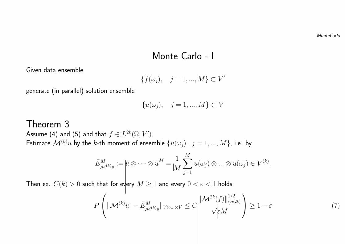
Monte Carlo - I
Given data ensemble
f(ωj), j = 1, ...,M ⊂ V ′
generate (in parallel) solution ensemble
u(ωj), j = 1, ...,M ⊂ V
Theorem 3Assume (4) and (5) and that f ∈ L2k(Ω, V ′).
Estimate M(k)u by the k-th moment of ensemble u(ωj) : j = 1, ...,M, i.e. by
EMM(k)u
:= u⊗ · · · ⊗ uM =1
M
M∑
j=1
u(ωj)⊗ ...⊗ u(ωj) ∈ V (k).
Then ex. C(k) > 0 such that for every M ≥ 1 and every 0 < ε < 1 holds
P
‖M(k)u − EM
M(k)u‖V⊗...⊗V ≤ C
‖M2k(f)‖1/2
V ′(2k)√εM
≥ 1− ε (7)

FEM
Monte Carlo - II
Lemma (Law of iterated logarithm in Hilbert spaces):
V separable Hilbert and X ∈ L2(Ω, V ). Then
lim supM→∞
∥∥∥XM − E(X)∥∥∥V
(2M−1 log logM)1/2≤ ‖X −E(X)‖L2(Ω,V ) with probability 1. (8)
Proof: Classical law of iterated logarithm: for real valued Y (ω) holds
lim supM→∞
∣∣∣Y M −E(Y )∣∣∣2
2M−1 log logM= VarY with probability 1.
Let Z := X−E(X). V separable⇒ w.l.o.g V = `2 = spanej∞j=1 and Y := (ej, Z) = Zj ∈ R. Apply (8) with
VarY = (ej ⊗ ej,M2Z) = (M2Z)j,j.
Add estimates for j = 1, 2, . . . and obtain
lim supM→∞
∑∞j=1 |Zj|2
2M−1 log logM≤
∞∑
j=1
(M2Z)j,j with probability 1.
Estimate ∞∑
j=1
(M2Z)j,j = E( ∞∑
j=1
(Z ⊗ Z)j,j
)=
Ω
∞∑
j=1
|Zj|2 dP (ω) = ‖Z‖2L2(Ω,V ) .

FEM
Monte Carlo - II
Application: P -a.s. convergence of MCM (Semidiscrete Case !)
Theorem 4
Let f ∈ L2k(Ω, V ′). Then
lim supM→∞
∥∥EMMku−Mku
∥∥V (k)
(2M−1 log logM)1/2≤ C ‖f‖kL2k(Ω,V ′) with probability 1.

FEM
Monte Carlo - IIIMCM - convergence in the absence of 2nd Moments
Theorem 5
Let k ≥ 1 and assume
f ∈ Lαk(Ω, V ′) for some α ∈ (1, 2].
Then ex. C such that for every M ≥ 1 and every 0 < ε < 1
P
(‖EMMku−Mku‖V (k) ≤ C
‖f‖kLαk(Ω,V ′)
ε1/αM 1−1/α
)≥ 1− ε (9)
So far: MCM assuming that Au = f solved exactly (“Semidiscrete MCM”).
Next: Galerkin FEM in V .

FEM
Galerkin FEM
Dense sequence of subspaces:
V0 ⊂ V1 ⊂ V2 ⊂ · · · ⊂ V` ⊂ V`+1 ⊂ . . . V
Galerkin FEM: given f ∈ Lk(Ω, V ′), find
uL(ω) ∈ Lk(Ω, V L) such that 〈vL, AuL(ω)〉 = 〈vL, f(ω)〉 ∀vL ∈ VL
Galerkin Projection: GL : V → VL defined by
∀v ∈ VL : 〈AGLu, v〉 = 〈f, v〉
is stable: ex. L0 > 0 s.t.
∀L ≥ L0 : ‖GLu‖V ≤ C‖u‖Vand converges quasioptimally:
∀L ≥ L0 ∀v ∈ VL : ‖u(ω)− uL(ω)‖V ≤ C‖u(ω)− v‖V P − a.e.ω ∈ Ω.
ConvRates
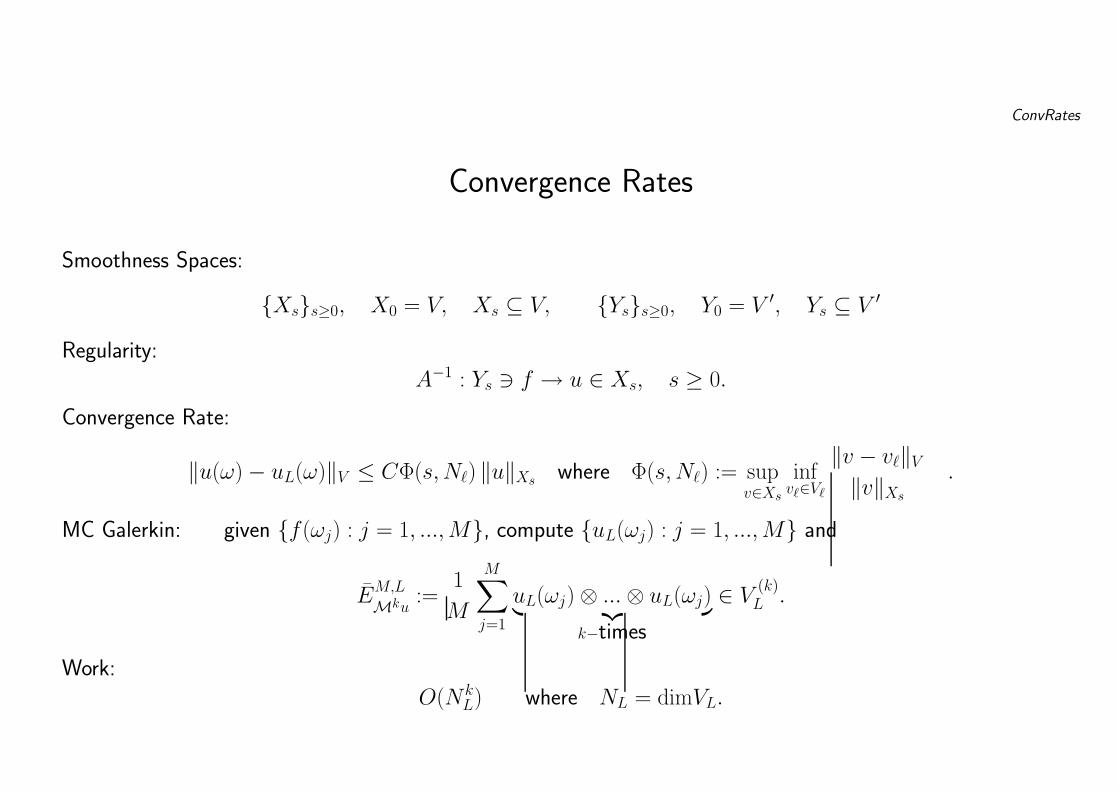
Convergence Rates
Smoothness Spaces:
Xss≥0, X0 = V, Xs ⊆ V, Yss≥0, Y0 = V ′, Ys ⊆ V ′
Regularity:
A−1 : Ys 3 f → u ∈ Xs, s ≥ 0.
Convergence Rate:
‖u(ω)− uL(ω)‖V ≤ CΦ(s,N`) ‖u‖Xs where Φ(s,N`) := supv∈Xs
infv`∈V`
‖v − v`‖V‖v‖Xs
.
MC Galerkin: given f(ωj) : j = 1, ...,M, compute uL(ωj) : j = 1, ...,M and
EM,L
Mku:=
1
M
M∑
j=1
uL(ωj)⊗ ...⊗ uL(ωj)︸ ︷︷ ︸k−times
∈ V (k)L .
Work:
O(N kL) where NL = dimVL.

WaveletFEM
Wavelet FEM (Cohen, Dahmen, Kunoth, Schneider, ...)
Wavelet Scale:
W0 := V0, V` = V`−1 ⊕W`, ` = 1, 2, . . . ,
Sparse Tensor Product Space (Smol’yak, Teml’yakov, Zenger, Griebel,...):
V(k)L =
∑
~∈Nk0|~|≤L
W`1 ⊗W`2 ⊗ · · · ⊗W`k .
Sparse Projection (quasi-interpolation):
P(k)L : V (k) → V
(k)L given by (P
(k)L v)(x) :=
∑
0≤`1+···+`k≤L1≤jν≤n`ν ,ν=1,...,k
v`1...`jj1...jk
ψ`1j1(x1) . . . ψ`kk (xk)
or
P(k)L =
∑
0≤`1+···+`k≤LQ`1 ⊗ · · · ⊗Q`k where Q` := P` − P`−1, ` = 0, 1, ... and P−1 := 0.

Wavelets
Biorthogonal Spline Wavelets in 1− d, degree p = 1.
V3
(Nodal basis)
W0
ψ10
W1
ψ11 ψ
21
W2
ψ12 ψ
22 ψ
32 ψ
42
W3
ψ13 ψ
23 ψ
33 ψ
43 ψ
53 ψ
63 ψ
73 ψ
83

WaveletFEM
Sparse Tensor Product Space(Zenger 1990, Griebel & Bungartz Acta Numerica 2004)
x
y
W0⊗ W
0W
1⊗ W
0
W0⊗ W
1

MCWaveletFEM
Monte Carlo IV – Sparse Monte Carlo FEM
Sparse Tensor Product MC estimate of Mku :
EM,L
Mku:=
1
M
M∑
j=1
P(k)L [uL(ωj)⊗ ...⊗ uL(ωj)] ∈ V (k)
L .
Work:
M × O(NL(log2NL)k−1) operations and NL(log2NL)k−1 memory
Theorem 6Assume 0 < α ≤ 1 and
f ∈ Lk(Ω, Ys) ∩ Lαk(Ω, V ′) for some 0 ≤ s < s0.
Then
Mku ∈ Xs ⊗ ...⊗Xs =: X(k)s
and there is C(k) > 0 such that for all M ≥ 1, L ≥ L0 and all 0 < ε < 1 holds
P(‖EM,L
Mku−Mku‖V (k) < λ
)≥ 1− ε
with λ = C(k)[Φ(s,NL)(logNL)(k−1)/2 ‖f‖kLk(Ω,Ys)
+ ε−1/αM−(1−1/α) ‖f‖kLαk(Ω,V ′)
].

SparseGalerkinFEM
Sparse Tensor Product FEM
Idea:
Compute Mku directly, without MC
Proposition 7Assume A satisfies (4), (5) and f ∈ Lk(Ω, V ′) for k > 1.
Then
(A⊗ ...⊗A)Z =Mkf , (10)
has a unique solution Z ∈ V (k) and
Z =Mku.
For f ∈ Lk(Ω, Ys), s > 0, holds
‖Mku‖Xs⊗...⊗Xs ≤ Ck,s ‖Mkf‖Ys⊗...⊗Ys, 0 ≤ s < s0, k ≥ 1
Regularity of Mku in spaces of mixed highest derivative!

SparseGalerkinFEM
Sparse Galerkin FEM
Since A may be indefinite, use
V(k)L,L0
:= V(k)L+L0
∩ V (k)L
instead of V(k)L where L0 is fixed as L→∞.
find ZL ∈ V (k)L+L0
such that⟨A(k) ZL, v
⟩=⟨Mkf, v
⟩∀v ∈ V (k)
L+L0. (11)
N.B. that
V(k)L ⊂ V
(k)L,L0⊂ V
(k)L+L0
.
Assume (4), (5) with
T : V → Yδ continuously for some δ > 0
Assume also the approximation property and f ∈ Lk(Ω, Ys), s > 0, k ≥ 1.
Then there exists L0 and cS > 0 such that for all L ≥ L0
inf0 6=u∈V (k)
L,L0
sup06=v∈V (k)
L,L0
〈A(k)u, v〉‖u‖V (k) ‖v‖V (k)
≥ 1
cS> 0 . (12)
In the case T = 0 this holds with L0 = 0.

Theorem 8
Then for all L ≥ kL0 sparse Galerkin approximation ZL of Mku is uniquely defined and
‖Mku− ZL ‖V⊗...⊗V ≤ C(k)Φ(s,NL)(logNL)(k−1)/2‖f‖Lk(Ω,Ys), 0 ≤ s < s0.
ZL can be computed with O(NL(logNL)m) work and memory.
Note: Tensor product Galerkin FEM gives
‖Mku− ZL ‖V⊗...⊗V ≤ C(k)Φ(s,NL)1/k‖f‖Lk(Ω,Ys), 0 ≤ s < s0
in O(NL) memory and work.
Conclusions
• Monte-Carlo Galerkin FEM: framework, convergence analysis
• Sparse Galerkin FEM: regularity in anisotropic spaces; sparse tensor product spaces
• Given data statistics, get solution statistics by deterministic computation
• trade stochasticity and MC for high-dimensionality + deterministic FEM
• Use sparse tensor products of wavelet spaces to avoid O(N kL) complexity
• Fast Matrix Vector Multiplication (Sch. & Todor: Numer. Math. 2003)
• a-priori and a-posteriori error estimates, adaptivity
→ framework of Cohen, Dahmen, DeVore in tensor product Besov spaces (Nitsche 2004)
Mk(u) ∈ Bαq (Lq(D))⊗q . . .⊗q Bα
q (Lq(D))
for arbitrarily large α with
q = [α/2 + 1/2]−1 < 1 indep. of k.
• Problems with stochastic boundary Γ (Harbrecht, R. Schneider, and CS. 2006)
• Problem with stochastic coefficients (Todor & CS. 2006)


![Sparse tensor discretization of elliptic sPDEs...accordingly “sparse tensor product stochastic Galerkin FEM”. In [7] we presented an efficient numerical sGFEM algorithm to solve](https://img.pdfslide.us/doc/110x75/5f77ae6cf8131406cd2a74b8/sparse-tensor-discretization-of-elliptic-spdes-accordingly-aoesparse-tensor.jpg)