Embed Size (px)
Citation preview

Wavelet-based Weighted LASSO and Screeningapproaches in functional linear regression
Yihong ZhaoDivision of Biostatistics, Department of Child and Adolescent Psychiatry,
New York University, New York, NY, USAHuaihou Chen
Division of Biostatistics, Department of Child and Adolescent Psychiatry,New York University, New York, NY, USA
R. Todd OgdenDepartment of Biostatistics, Columbia University, New York, NY, USA
1

Author’s Footnote:
Yihong Zhao is Assistant Professor at Division of Biostatistics, Department of Child and Adoles-cent Psychiatry, New York University Langone Medical Center (Email: [email protected]);Huaihou Chen is Postdoctral Fellow at Division of Biostatistics, Department of Child and Adoles-cent Psychiatry, New York University Langone Medical Center (Email: [email protected]),and R. Todd Ogden is Professor of Biostatistics at Department of Biostatistics, Columbia Univer-sity (Email: [email protected]).
2

Abstract
One useful approach for fitting linear models with scalar outcomes and functional pre-dictors involves transforming the functional data to wavelet domain and converting the datafitting problem to a variable selection problem. Applying the LASSO procedure in this sit-uation has been shown to be efficient and powerful. In this paper we explore two potentialdirections for improvements to this method: techniques for pre-screening and methods forweighting the LASSO-type penalty. We consider several strategies for each of these directionswhich have never been investigated, either numerically or theoretically, in a functional linearregression context. The finite-sample performance of the proposed methods are comparedthrough both simulations and real-data applications with both 1D signals and 2D imagepredictors. We also discuss asymptotic aspects. We show that applying these procedures canlead to improved estimation and prediction as well as better stability.
Keywords: functional data analysis, penalized linear regression, wavelet regression, adaptiveLASSO, screening strategies
1 Introduction
Substantial attention has been paid to problems involving functional linear regression model
yi = α +
∫ 1
0
Xi(t)η(t)dt+ εi, i = 1, . . . , n, (1)
where the response yi and the intercept α are scalar, the predictor Xi and the slope η are square-
integrable functions in L2 ([0, 1]), and the errors εi are independent and identical normally dis-
tributed with mean 0 and finite variance σ2. The literature on functional linear regression is grow-
ing. A sampling of papers examining this situation and various asymptotic properties includes
Cardot et al. (2003), Cardot and Sarda (2005), Cai and Hall (2006), Antoniadis and Sapatinas
(2007), Hall and Horowitz (2007), Li and Hsing (2007), Reiss and Ogden (2007), Muller and Yao
(2008), Crainiceanu, Staicu, and Di (2009), Delaigle, Hall, and Apanasovich (2009), James et al.
(2009), Crambes, Kneip, and Sarda (2009), Goldsmith et al. (2012), and Lee and Park (2012). A
potentially very useful idea in fitting models involving functional data is to transform functional
data via wavelets. Recent literature on functional data analysis in the wavelet domain includes
Amato, Antoniadis, and De Feis (2006), Wang, Ray, and Mallick (2007), Malloy et al. (2010), Zhu,
Brown, and Morris (2012), and Zhao et al. (2012).
Wavelet-based LASSO (Zhao et al., 2012) has been proposed as a powerful estimation ap-
proach for fitting the model (1). It works by transforming the functional regression problem to a
variable selection problem. Functional predictors can be efficiently represented by a few wavelet
coefficients. After applying discrete wavelet transform (DWT), techniques such as LASSO (Tib-
shirani, 1996) can then be applied to select and estimate those few important wavelet coefficients.
3

Wavelet-based LASSO method is well suited for the situation in which the η function has spatial
heterogeneity and/or spiky local features. Although wavelet-based LASSO method has good pre-
diction ability, we observed from simulation studies that the functional coefficient estimates often
show anomalously large point-wise variability.
The purpose of this article is to explore two potential directions for improvements to the
wavelet-based LASSO: methods for weighting the LASSO-type penalty and techniques for pre-
screening. Although weighting the L1 penalty terms and adding a pre-screening step have been
widely studied in linear regression model setting, these strategies have never been investigated,
either numerically or theoretically, in a functional linear regression model context. In this study,
we first demonstrate weighted version LASSO can improve both prediction ability and estimation
accuracy. In linear regression, although LASSO shows good prediction accuracy, it is known to
be variable selection inconsistent when the underlying model violates certain regularity conditions
(Zou, 2006; Zhao and Yu, 2006). Meinshausen and Buhlmann (2006) prove that the prediction
based tuning parameter selection method in LASSO often results in inconsistent variable selection,
and consequently the final predictive model tend to include many noise features. To improve
LASSO’s performance, Zou (2006) proposed to add weights to the L1 penalty terms where weights
were defined as ordinary least square (OLS) estimates. Later, (Huang et al., 2008) considered the
magnitudes of correlation coefficient between the predictor and the response as the weights. Both
approaches were shown to have better variable selection consistency. In functional linear model
setting, wavelet-based LASSO suffers from the same difficulty resulting from inconsistent selection
of wavelet coefficients. We extend weighted LASSO methods to functional linear regression in
the wavelet domain, with the hope that this can improve estimation accuracy by penalizing less
important variables more than more important ones. In functional linear regression, the predictors
are often curves densely sampled at equally spaced points. That is the number of data points
can be much larger than the sample size resulting in a “large p small n” problem. Therefore,
using OLS estimates as weights is not feasible in general. We propose two new weights. The
first weighting scheme uses information from the magnitudes of wavelet coefficients, whereas the
second one is based on sample variances of wavelet coefficients. Those two weight schemes are
fundamentally different from other weighting schemes in that the importance of each predictor is
ranked without consideration of its relationship with response variable. Our results show that the
wavelet-based weighted LASSO not only provide great prediction accuracy, but also significantly
improve estimation consistency.
Second, we show that incorporating a screening step before applying a LASSO-type penalty
4

in the wavelet domain can improve both prediction ability and estimation accuracy. Adding a
screening step to wavelet-based LASSO can be important. For example, it is increasingly common
in practice to have functional predictors with ultra-high dimensionality. The challenge of sta-
tistical modelling using ultra-high dimensional data involves balancing three criteria: statistical
accuracy, model interpretation, and computational complexity (Fan and Lv, 2010). For example,
Shaw et al. (2006) used serial image data to study how longitudinal changes in brain develop-
ment in young children with attention deficit hyperactivity disorder (ADHD) can predict relevant
clinical outcomes. In such a case, it is desirable to apply a screening step before model fitting.
With 2D images of size 128 × 128 as predictors, it is necessary to deal with more than 16, 000
predictors in the wavelet domain. Therefore it is of critical importance to reduce dimensionality
to a workable size. In this paper, we investigate some screening approaches that would effectively
reduce computational burden while the reduced model still contains all important information
with high probability.
The rest of this article is organized as follows. In Section 2, we propose two versions of weighted
LASSO in wavelet domain analysis. We then introduce some screening approaches to functional
linear models. We show their statistical properties in Section 3 and use simulation studies and
real data examples to demonstrate finite sample performance of the proposed methods in Section
4. Section 5 concludes this paper with some discussions.
2 Methods
In this section, we introduce wavelet-based weighted LASSO with different weighting schemes
in the penalty term and discuss some screening strategies that can be applied to wavelet-based
functional linear model. We assume readers have certain familiarity with wavelet transform.
Readers without this background can refer to Ogden (1997), Vidakovic (1999), and Abramovich,
Bailey, and Sapatinas (2000) for a comprehensive overview of wavelet applications in statistics.
2.1 Wavelets
Let φ and ψ be a compactly supported scaling function and detail wavelet, respectively with∫φ(t)dt = 1. Define φjk = 2j/2φ(2j − k) and ψjk = 2j/2ψ(2j − k). For a given decomposition level
j0, {φj0k : k = 0, . . . , 2j0 − 1} ∪ {ψjk : j ≥ j0, k = 0, . . . , 2j − 1} forms a basis set of orthonormal
wavelets for L2 ([0, 1]). Let {z′ij0k = 〈Xi, φj0k〉 , k = 0, . . . , 2j0 − 1} and {zijk = 〈Xi, ψjk〉 , j =
j0, . . . , log2(N)− 1, k = 0, . . . , 2j − 1}. By discrete wavelet transform (DWT), the functional pre-
5

dictor Xi sampled at N equally spaced points can be represented by a set of N wavelet coefficients:
Xi =2j0−1∑k=0
z′ij0kφj0k +
log2(N)−1∑j=j0
2j−1∑k=0
zijkψjk = W TZi,
where N is a power of two, W is an orthogonal N × N matrix associated with the orthonormal
wavelet bases, and Zi is an N × 1 vector of wavelet coefficients from DWT of Xi. Similarly, the
wavelet series of the coefficient function η can be written as
η =2j0−1∑k=0
β′j0kφj0k +
log2(N)−1∑j=j0
2j−1∑k=0
βjkψjk = W Tβ,
where β′j0k = 〈η, φj0k〉, βjk = 〈η, ψjk〉, and β is an N × 1 vector of wavelet coefficients from DWT
of η.
In this paper, we require an orthonormal wavelet basis on [0, 1] such as those in Daubechies’
family. Wavelet transform is a compelling choice of such transform mainly due to its great com-
pression ability, i.e, functions can be represented by relatively few non-zero wavelet coefficients.
Penalized regression methods can be readily extended to functional linear model once functional
predictors are transformed into wavelet domain.
2.2 Wavelet-based Weighted LASSO
The general form of a linear scalar-on-function model is given in (1). For simplicity, we will drop
the term α from equation (1). The intercept α can be estimated by α = Y −∫ 1
0X(t)η(t)dt, where
Y and X are sample means of response and functional predictor, respectively. We assume each
functional predictor Xi and the coefficient function η have a sparse representation in the wavelet
domain. By applying the DWT to functional data at a primary decomposition level j0, we can
obtain a discrete version of model (1) expressed as
yi = XTi β + εi =
N∑h=1
zihβh + εi, i = 1, . . . , n. (2)
A natural estimation of β in equation (2) can be obtained via penalized regression:
β = arg minβ
1
n
n∑i=1
(yi −
N∑h=1
zihβh
)2
+N∑
h=1
λ
wh
|βh|, (3)
where wh are some user-defined positive weights. Various choices of weights have been proposed in
linear regression model setting. For example, the LASSO (Tibshirani, 1996) used constant weights
wh = 1. Weights wh = |β0h| are considered by Zou (2006) where each β0
h is an OLS estimate of the
6

corresponding term in the model, while Huang et al. (2008) considered correlation based weights
with wh =
∣∣∣∣( n∑i=1
zihyi
)/
(n∑
i=1
z2ih
)∣∣∣∣.In this paper, we propose two new weighting schemes specific to wavelet-based penalized re-
gression method. The weights in (3) can be defined as:
1. wh = θh, where θh = 1n|
n∑i=1
zih|; or
2. wh = σ2h, where σ2
h = 1n−1
n∑i=1
(zih − zh)2 and zh is the sample mean of the hth wavelet
coefficients.
The proposed methods are mainly motivated by shrinkage-based estimators in nonparmetric re-
gression with wavelets (Donoho and Johnstone, 1994; Donoho at al., 1996). That is, the empirical
wavelet coefficients with magnitudes less than a threshold value C contain mostly the noise and
thus ignorable in estimating η. When applied to L1-type penalty in wavelet-based approaches,
weighting each wavelet coefficient by its magnitude induces threshold-like effect which eventually
leads to adaptive regularization.
The rationale for using sample variance of wavelet coefficients as weights comes from Johnstone
and Lu (2009). They pointed out that wavelet coefficients with large magnitudes typically have
large sample variances, which also agrees with what we have observed in real data examples.
In addition, variables with low variability would provide limited predictive power to the outcome
variable in regression analysis. Therefore, weighting by the sample variances of wavelet coefficients
could effectively separate important variables from unimportant ones. We expect that weighting
by sample variance would similarly introduce adaptive regularization to L1-type penalty.
The data-dependent weight wh is critical in terms of consistency of variable selection and model
estimation for the LASSO-type estimator. The weight function should be chosen adaptively to
reduce biases due to penalizations. Ideally, as the sample size increases, we would want the weights
for less important, noisy predictors to go to infinity and the weights for important, nonzero ones
to converge to a small constant (Zou, 2006). That is, adaptive regularization should effectively
separate important nonzero wavelet coefficients from the unimportant ones.
2.3 Screening strategies
When the data dimensionality is very high, it is natural to perform screening before model fit-
ting. We consider four approaches for the wavelet-based methods: 1) Screening by correlation,
7

2) Screening by stability selection, 3) Screening by variance, and 4) Screening by magnitude of
wavelet coefficient.
Screening by Correlation: Fan and Lv (2008) propose to select a set of important variables
through a Sure Independence Screening (SIS) procedure. Specifically, the SIS procedure involves
selecting covariates based on the magnitudes of their sample correlations with the response vari-
able. Only the selected covariates will be used for further analysis. The SIS step significantly
reduces computational complexity. They showed that the SIS procedure can reduce the dimen-
sionality from an exponentially growing number down to a smaller scale, while the reduced model
still contains all the variables in the true model with probability tending to 1.
Screening by Stability Selection: Meinshausen and Buhlmann (2010) demonstrate that variable
selection and model estimation improve markedly if covariates are first screened by the stability
selection procedure. The stability selection procedure involves selecting variables based on their
maximum frequencies of being included in models built on perturbed data over a range of regular-
izations. They claimed that, with stability selection, the randomized LASSO can achieve model
selection consistency even if the irrepresentability condition is not satisfied. In this paper, we will
use a similar approach to screen out less important wavelet coefficients before model fitting. Using
wavelet-based LASSO as an example, we resample dn/2e individuals from the data, fit the wavelet-
based LASSO, and the variables remaining in the model are selected by 5-fold cross-validation.
We repeat this process B times and the variables with their proportions of inclusion less than a
threshold value (π) will be excluded from further analysis.
Screening by Variance: For principal component analysis (PCA) of signals with ultrahigh
dimension, Johnstone and Lu (2009) assert that some initial reduction in dimensionality is desirable
and this can be best achieved by working in wavelet domain in which the signals have sparse
representations. Screening by variance before applying PCA algorithm can improve estimation.
We will extend this to the linear scalar-on-function regression model. The wavelet coefficients with
small sample variances will be excluded from the model.
Screening by Magnitudes of Wavelet Coefficients: Wavelet coefficients with large magnitude
tend to have a large presence in the predictor functions and thus may play a role in predicting the
outcome. Let M = {1 ≤ l ≤ N : θl 6= 0} and θ(1) ≥ θ(2) ≥ · · · ≥ θ(N) be the sample magnitudes of
wavelet coefficients. For a given k, the selected subset M = {l : θl ≥ θ(k)}.
8

2.4 Algorithm
In the previous two sections, we proposed two schemes for weighted LASSO which are specific
to wavelet domain analysis and extended some screening strategies to wavelet-based methods for
functional linear model. In general, the wavelet-based penalized regression can be implemented
as following:
1. Transform functional predictors into wavelet domain.
2. Select a subset of important wavelet coefficients by one of the following criteria: a) selecting
all coefficients; b) selecting k coefficients with the largest sample variances; c) selecting k
coefficients with the largest sample magnitudes; d) selecting k coefficients with the largest
sample correlations in magnitude; or e) selecting k coefficients by stability selection.
3. Variable selection and model estimation by LASSO-type algorithm where the weight wh, h =
1, . . . , N in (3) is defined by one of the following: a)wh = 1; b)wh = θh; c) wh = σh; or d)
wh =
(n∑
i=1
zihYi
)/
(n∑
i=1
z2ih
)4. Transform coefficient estimations back to the original domain by inverse wavelet transform.
Extension of the above methods to functional linear model with 2D or 3D image predictor is
straightforward by performing 2D or 3D wavelet decomposition to image predictors.
2.5 Tuning parameter selection
Two tuning parameters λ and j0 involved in the wavelet-based weighted LASSO methods. The
tuning parameter λ controls the model sparsity. It must be positive. All variables are retained in
the model for λ → 0, and the model becomes empty as λ → ∞. The other tuning parameter j0
ranges from 1 to log2(N)− 1. The choice of j0 controls the optimal level of wavelet decomposition
for the functional data. In this study, we choose the values of λ and j0 by 5-fold cross-validation
such that the optimal combination of λ and j0 would produce the lowest cross-validated residual
sum of squares over a grid values of λ and j0.
If a screening step is applied before running the desired method, the number of features selected
for further analysis (i.e., k) needs to be chosen as well. This value can be chosen by cross-validation,
but we do not recommend it. In practice, the results are relatively insensitive to the exact value
of k, and we don’t want to exclude too many variables in the screening step. Typically, we would
select k such that the first k wavelet coefficients would explain 99.5% of total variability in the
9

data. Due to great compression ability of wavelets, we notice this number is often smaller than
n− 1 in our simulation studies.
3 Asymptotic properties
In this section, we will provide some theoretical support of the wavelet-based adaptive LASSO
method with magnitudes of wavelet coefficients as weights (i.e, wh = θh in equation (3)). In
addition, we will study the correct selection property of one screening approach: selection by
magnitudes of wavelet coefficients.
3.1 Consistent Estimation
We investigate asymptotic properties of wavelet-based adaptive LASSO estimator when the curves
are increasingly densely observed (N →∞) as the sample size increases (n→∞). After applying
a screening step (i.e., selection by magnitudes of wavelet coefficients), the dimensionality of the
functional predictor in wavelet domain reduced from Nn to kn. Here we subscript quantities that
vary with the sample size n. Consequently, equation (2) becomes
yi =kn∑h=1
zihβh + ε∗i , i = 1, . . . , n, (4)
where ε∗i = εi + ξi, and ξi =∑Nn
h=knzihβh is the screening error.
Let Zkn be a n × kn matrix, where the columns of Zkn are the kn wavelet coefficients that
remain after screening. Let Hn = {h : |βh| ≥ Cn} with Cn > 0, and the cardinality is Sn = |Hn|.
Let ρkn be the smallest eigenvalue of Σkn = 1nZT
knZkn . In addition, let ζHn = min
h∈Hn
|βh| be the
smallest magnitude of the coefficients. Following Lee and Park (2012), who proposed a general
framework for penalized least squared estimation of η in equation (1), we make the following
assumptions:
(a1) After the screening step, kn is larger than the greatest index in the set Hn.
(a2)∑
h∈Hnn1/2λn/θh = op(1).
(a3) η is a q times differentiable function in the Sobolev sense (i.e. η ∈ W q[0, 1]), and the wavelet
basis has p vanishing moments, where p > q.
(a4) (∑∞
h=0 |〈η, ψh〉|r)1/r <∞ for some r < 2.
10

Assumption (a1) is satisfied if kn → ∞ as n → ∞. Also, due to correct selection property of
the screening method (see section 3.2), for sufficiently large n, the selected subset of kn wavelet
coefficients includes nonzero ones with probability tending to one. Assumption (a2) is satisfied if
n1/2λnSnζ−1Hn→ 0.
Theorem 1. Let η be the estimated coefficient function for model (2). Let kn be the number of
predictors remaining in the model after screening step, and ρkn be the smallest eigenvalue of Σkn.
If assumptions (a1)-(a4) hold, then
‖ ηn − η‖ 2L2 = Op
(knnρ2kn
)+ o(k1−2/rn ) + o(N−2qn ).
The proof is provided in the appendix. Note Theorem 1 relies on correct selection of nonzero
wavelet coefficients in the screening step. If no screening is applied prior to model fitting, then
‖ ηn − η‖ 2L2 = Op
(Nn
nρ2Nn
)+ o(k1−2/rn ) + o(N−2qn ),
where ρNn is the smallest eigenvalue of ΣNn = 1nZT
NnZNn and ZNn is an n×Nn matrix of all wavelet
coefficients. Clearly, if the screening strategy selects all nonzero wavelet coefficients with probably
tending to 1, the proposed method with screening step improves the estimation compared to the
one without screening step.
3.2 Probability of false exclusion
Johnstone and Lu (2009) showed that the probability that the selected subset does not contain
wavelet coefficients with the largest sample variances is polynomially small. In this section, we
will show that the selected subset M contains the largest population magnitudes with probability
tending to 1. We assume each wavelet coefficient Zh follows a normal distribution, i.e.
Zh ∼ N(µh, σ2h), h = 1, . . . , N. (5)
Let θh = |µh| and θh = 1n|∑n
i=1 zih|. Without loss of generality, let the population magnitude be
θ1 ≥ θ2 ≥ · · · ≥ θN , and the ordered sample magnitude be θ(1) ≥ θ(2) ≥ · · · ≥ θ(N). We include all
indices l in M = {1 ≤ l ≤ N : θl 6= 0}. Following Johnstone and Lu (2009), a false exclusion (FE)
occurs if any variable in M is missed:
FE =⋃l∈M
{l /∈ M
}=⋃l∈M
{θl < θ(k)}
11

Theorem 2. Assume (5), let Ch = σh/θh, h = 1, 2, . . . , N, where 0 < Ch < C0. Let Φ(.) be the
cumulative distribution function of a standard normal variable. With γn =√log(n)/n, θk = bγn
where b > 0, a suitably chosen constant d > 1, and a subset of k variables are selected, an upper
bound of the probability of a false exclusion is given by
P (FE) ≤ (N − k + 1) Φ
(−√nγn/θkC0
)+ (N − k + 1) Φ
(−√n(2 + γn/θk)
C0
)+ Φ
(√n(1/d− 1)
C0
)The proof of this theorem, following the steps in proof of Theorem 3 by Johnstone and Lu
(2009), is provided in the appendix. The probability of false exclusion is a function of the number
of observation points N , the sample size n, the size of the selected variable set k, the smallest
wavelet coefficient magnitude in the selected model θk, and the signal to noise ratio as estimated by
coefficient of variation C0. As an example, if the size of the selected set k = 50, while N = 1000,
d = 2, and b = 0.75, then P (FE) ≤ 0.05 for C0 = 3 with n = 100. The probability of false
exclusion reduces to 0.009 if the sample size n increases to 200.
4 Numerical studies
In this section, we perform simulations to study finite sample performance of wavelet-based
weighted LASSO as well as different screening approaches in functional linear regression. To
simplify notations in figure legends and labels, as well as in Tables, we use “LASSO” to repre-
sent wavelet-based LASSO approach, and “Wv”, “Wm”, and “Wc” for wavelet-based weighted
LASSO method with variance, magnitudes of wavelet coefficients, and magnitudes of correlation
coefficients as penalty weights, respectively.
4.1 Simulation study - 1D functional predictor
We employ similar settings as those in Zhao et al. (2012). Specifically, functional predictors, xi(t),
t ∈ (0, 1), are generated from a Brownian bridge stochastic process. That is, X(t) is a continuous
zero-mean Gaussian process both starting and ending at 0 and with Cov(X(t), X(s)) = s(1 − t)
for s < t. The true coefficient function is “heavisine” (see Figure S1 in supplementary materials).
Performance of the proposed methods is compared under different noise levels, where signal to
noise ratio (SNR), measured by the squared multiple correlation coefficient of the true model, is
set to 0.2, 0.5, and 0.9 respectively. The curve is sampled at N = 1024 equally spaced time points.
We carry out 200 simulations for each setting of the parameters with the sample size (n) fixed
at 100 for each run. The discrete wavelet transform is performed using “wavethresh” package
12

(Nason, 2010) in R 2.15.1. In this study, we use “Daubechies Least Asymmetric family” with
periodic boundary handling and the filter number is set to 4.
The L1 penalty parameter λ and the wavelet decomposition level j0 are selected by 5-fold cross
validation. The size k of the set of selected variables in the screening step should be determined
from the data. In this study, we restrict the maximum number of selected wavelet coefficients at
the screening step to be n−1 for all screening approaches except for screening by stability selection.
When screening by stability selection, for each dataset, we run proposed methods 400 times in
random subsamples of size dn/2e, where the random subsamples are drawn without replacement.
Variables shown in the final models at least 80% of the time are included for further analysis after
screening step.
Prediction and Estimation: Weighted versus Unweighted LASSO
Performance of various methods is compared according to their prediction ability and estimation
accuracy. The prediction ability is measured by the mean absolute error of prediction (MAE)
1n
∑ni=1 |Z
Ti β − ZT
i β|, while the estimation accuracy is measured by mean integrated squared
error (MISE) = 1N
∑Nh=1(βh − βh)2.
Figures 1 and 2 along with Table 1 show MAEs and MISEs for the proposed methods in
combination with different screening approaches. Weighted LASSO methods clearly give smaller
prediction errors and better estimation accuracy than unweighted LASSO does. When SNR is high
(i.e., R2 = 0.9), all three weighted LASSO approaches have similar prediction accuracy as that
of the unweighted LASSO. However, the weighted LASSO methods result in about 15% − 19%
reduction in prediction error for smaller SNR. The prediction errors from unweighted methods
when R2 = 0.2 are even smaller than those from unweighted LASSO when R2 = 0.5. Compared
to the unweighted LASSO, the weighted methods show around 65% − 84% reduction in MISEs,
depending on the weighting schemes and SNRs.
Mean and Standard deviation functions obtained from 200 simulated datasets are plotted in
Figure 3. Although unweighted LASSO shows great prediction accuracy, the mean estimated
coefficient function η does not approximate the truth well and it has large variability. In contrast,
weighted methods clearly improve estimation accuracy and the resulting η tends to be more
stable across different simulated datasets, as demonstrated by much lower point-wise variability
in functional coefficient estimations. The point-wise standard deviations from unweighted LASSO
range from 10 to 30 at most points, while those from weighted LASSO methods are generally in the
range of 1 to 4. It is not surprising to observe the conflict between good prediction and consistent
13

Table 1: MAE and MISE based on 200 simulations when η is “heavisine”
MAE MISE
Method Screening R2 = 0.9 R2 = 0.5 R2 = 0.2 R2 = 0.9 R2 = 0.5 R2 = 0.2
LASSO None 1.25 1.87 2.22 1.89 3.91 4.63
LASSO Variance 1.16 1.58 1.82 0.25 0.76 1.42
LASSO Absolute mean 1.16 1.58 1.82 0.20 0.78 1.60
LASSO Correlation 1.23 1.91 2.29 1.74 3.78 4.57
LASSO Stability 1.17 1.65 1.93 0.13 0.86 1.50
Wv None 1.20 1.58 1.83 0.30 1.10 1.56
Wv Variance 1.12 1.57 1.84 0.12 0.65 1.88
Wv Absolute mean 1.12 1.57 1.84 0.12 0.64 1.51
Wv Correlation 1.15 1.64 1.93 0.28 1.27 2.09
Wv Stability 1.16 1.63 1.89 0.13 0.71 1.47
Wm None 1.17 1.58 1.82 0.39 0.99 1.37
Wm Variance 1.16 1.60 1.84 0.21 0.74 1.50
Wm Absolute mean 1.16 1.61 1.84 0.23 1.29 1.89
Wm Correlation 1.17 1.65 1.99 0.17 1.41 2.62
Wm Stability 1.18 1.65 1.89 0.18 0.90 1.52
Wc None 1.27 1.59 1.85 0.36 1.01 1.66
Wc Variance 1.15 1.64 1.93 0.28 1.27 2.09
Wc Absolute mean 1.16 1.64 1.92 0.28 1.40 2.13
Wc Correlation 1.19 1.88 2.28 1.03 3.58 4.53
Wc Stability 1.16 1.64 1.96 0.12 0.75 2.24
14

estimation in the unweighted LASSO. Meinshausen and Buhlmann (2006) showed that, in linear
regression model, the optimal λ chosen by cross-validation criterion in LASSO often resulted in
inconsistent variable selection. This is also observed with unweighted LASSO.
Effects of screening on model estimation
From Table 1, screening by variance, wavelet coefficient magnitude, or stability selection results in
significant improvement of prediction and estimation accuracy for LASSO. The prediction errors
are reduced by up to 20% with the screening step, and most significantly, the estimation errors are
dropped by up to 93%. It should be noted that those three screening approaches show limited or
no improvement in terms of both prediction error and the estimation accuracy when the resulting
method is fit using weighted LASSO methods.
Irrespective of signal to noise ratio, the gain of adding a screening step is substantial in terms of
stability of coefficient function estimation in most settings. Figure 4 and Figures S2, S3, and S4 (in
supplementary materials) demonstrate that the screening step results in significant improvements
in reducing coefficient function estimation variability. This effect of screening on the stability
of coefficient function estimation is most impressive for LASSO method in which the point-wise
standard deviations were reduced from a wide range of values (e.g., 10− 50) to values less than 2.
In general, screening by magnitude and screening by variance of wavelet coefficient perform
similarly, and they tend to be better than the other screening methods in terms of both prediction
and estimation accuracy. Screening by stability selection generally gives desirable results but it is
computationally expensive. Compared to the other strategies, screening by correlation performs
worst in terms of both prediction error and estimation accuracy. It shows very limited improvement
over the underlying methods when signal to noise ratio (SNR) is high and it deteriorates prediction
when SNR is low. This is true regardless of the weighting scheme applied. It should be noted that
when the model-fitting method is unweighted LASSO or LASSO with magnitudes of correlation
coefficients as penalty weights, screening by correlation does not help improve estimation accuracy
and estimation stability. One possible reason for this is that there may be a group of highly
correlated wavelet coefficients after the pre-screening step, and LASSO tends to select only one
variable from the group, an observation made by Zou and Hastie (2005).
15

4.2 Simulation study - 2D image predictor
Following Reiss et al. (2014) and Goldsmith et al. (2014), we simulate 500 images based on
the first 332 weighted principal components from a subsample of ADHD-200 data (ADHD-200
Consortium, 2012), where weights are randomly chosen from N(0, λj) with λj, j = 1, . . . , 332,
being the corresponding jth eigenvalue. The true coefficient image (η1) is generated based on the
first five principal components computed from the ADHD-200 data. Similar to settings for 1D
functional predictor, we generate 200 sets of continuous outcomes with n = 500 and the signal to
noise ratio is controlled at 0.2, 0.5, and 0.9, respectively.
Prediction ability and estimation accuracy are compared based on criteria defined in Section
4.1. The prediction errors from 200 simulated data can be found in Table S1 and the mean
estimated image coefficients in Figure S5 in the supplementary materials. LASSO weighted by
the magnitudes of wavelet coefficients shows slightly better performance in terms of estimation
accuracy, though it does not generally show better prediction.
4.3 Real data analysis
The wheat data: 1D functional predictor The wheat dataset consist of 100 samples of Near infrared
spectroscopy (NIR) spectrum measured from 1100 nm to 2500 nm in 2-nm intervals (Kalivas,
1997). The aim of this study is to establish whether NIR spectra of wheat samples can be used
to predict the wheat quality parameters (e.g., the moisture and the protein contents). In our
analysis, we use the once-differenced spectra to correct for a baseline shift. The spectra are then
linearly interpolated at 512 equally spaced points.
The ADHD-200 data: 2D image predictor This dataset comes from the recent ADHD-200
Global Competition (ADHD-200 Consortium, 2012). The image predictors are maps of fractional
amplitude of low-frequency fluctuations (fALFF) from resting-state functional magnetic resonant
images (rs-fMRI), where fALFF indicates the intensity of regional brain spontaneous activities and
is defined as the ratio of BOLD signal power spectrum within low frequency range (i.e., 0.01−0.08
Hz) over that of entire frequency range. The 2D image predictors are obtained from the slices for
which mean fALFF has the largest variability across voxels. We have 333 samples in this study.
In our study, we are trying to determine the relationship between brain measurements and IQ. In
this study, IQ was first regressed on age, gender, and handedness. The residuals were used as the
new responses.
16

Prediction, estimation, and statistical inference
Prediction accuracy The data are randomly split into two halves with the first half used as training
data and the second half as testing data. We repeat this process 10 times. The mean absolute
prediction errors summed over testing datasets are reported in Table S2 for the wheat data and
Table S3 for the ADHD 200 data. In both datasets, MAEs from the wavelet-based weighted
methods are comparable to or smaller than that from the wavelet-based LASSO method, and the
screening step generally results in smaller MAEs compared to those from the underlying methods.
Coefficient function estimation and statistical inference
The wheat data: Figure 5 show the estimated functional coefficients and their corresponding
confidence intervals when the outcome measure is moisture content. Consistent with what we
find in simulation studies, the functional coefficient estimations from the wavelet-based weighted
LASSO methods are more stable/consistent. The estimated coefficient functions (Rows 1 and
2 in Figure 5) suggest a negative relationship between moisture contents and the intensity of
transmission of NIR radiation from the spectral range 1900- 2150 nm.
Confidence intervals on ω(t) can be generated using non-parametric bootstrapped based approach.
We used B = 1000 nonparametric bootstrap samples of matched pairs Yi, Xi(t) and reestimating
ω(t). The pointwise estimators for the mean coefficient function ω(t) and the standard deviation of
ω(t) are ω(t) =∑B
i=1 ωb(t)/B and s(t) =∑B
i=1 (ωb(t)− ω(t))2 /B respectively. The 95% pointwise
confidence intervals can be obtained by calculating ω(t) ± 1.96 ∗ s(t). The 95% joint confidence
intervals take the form ω(t) ± q0.95 ∗ s(t), where q0.95 is the 95% quantile of Mb, b = 1, 2, . . . B.
Here Mb is the maximum over the entire range of t values of the standardized mean realizations
for bth bootstrapped sample. Detailed algorithm for calculating Mb can be found in Crainiceanu
et al. (2012b). A permutation based test developed by James et al. (2009) can be used for testing
statistical significance of the relationship between the NIR spectrum of wheat and their moisture
contents.
Rows 3 and 4 in Figure 5 illustrate the permutation test results. The horizontal line with solid
dot indicates the observed R2 for each method applied to the wheat data. Other dots in the each
plot are permuted R2. We permuted the response variable 1000 times and calculated a permuted
R2 for each permutation. All permuted R2s were well below the observed R2, especially when Wm
and Wv methods are employed, providing very strong evidence of a true relationship between
the NIR spectrum and wheat moisture content. We do believe in this strong relationship as the
17

application of near infrared spectroscopic technique for the quantitative analysis of food products
is nowadays well established. Note there is discrepancy in bootstrap estimates and permutation
test of zero relationship when LASSO or Wc method is applied, providing evidence that instability
estimation of LASSO and Wc deteriorates the performance of bootstrapping method.
The ADHD-200 data: We plot the mean coefficient images in Figure 6 (Row 1) for ADHD study.
The mean coefficient images from Wm and Wv are more sparse and arguably more interpretable
than those from wavelet-based LASSO and Wc. The algorithm in Crainiceanu et al. (2012b)
can be extended in 2D image setting to obtain the pointwise and joint confidence intervals for
coefficient image. Row 2 in Figure 6, derived from 95 % pointwise confidence intervals, indicate
brain regions where there are significant association between image predictor and response variable
IQ.
Figure 6 also illustrate the permutation test results for the ADHD data. Similarly, we observed
discrepancy in bootstrap estimates and permutation test of zero relationship when LASSO or Wc
method is applied. From the real data examples, the original wavelet-based LASSO and the
proposed weighted versions show agreement in terms of permutation test results and discrepancy
in bootstrap based confidence interval estimations. This is expected because permutation tests
are based on how well the predictor predicts the response and both the original method and
the proposed methods in general show excellent prediction ability. In contrast, bootstrap-based
approaches perform well only if the underlying methods can produce accurate coefficient estimation
with small variance. The original wavelet-based LASSO are unstable in coefficient estimation,
therefore it deteriorates the performance of bootstrap-based approach.
5 Discussion
The primary contributions of this paper are the investigations of several strategies in the wavelet-
based LASSO context for (a) screening coefficients and for (b) coefficient-specific weighting of
L1 penalizations. These various strategies have been studied both in terms of estimation and
prediction as well as in terms of estimator stability. Additionally, this paper illustrates one of
the strengths of wavelet methods in this context: that the basic extension of functional data
methods from one-dimensional signals to two- or three-dimensional images is straightforward both
conceptually and computationally. One important point to keep in mind is that, due to the greater
natural dimensionality of imaging data, this extension merits further study.
Wavelet-based LASSO shows great prediction but relatively poor estimation accuracy, espe-
18

cially in the setting in which the “irrepresentability condition” is violated. In this study, we showed
that this procedure can be improved by adding a pre-screening step prior to the model fitting or,
alternatively, by using a weighted version of wavelet-based LASSO. The proposed approach in gen-
eral shows better prediction ability as well as improved estimation accuracy as compared to the
wavelet-based LASSO. An additional advantage is more stable coefficient function estimations,
as evidenced by results from a simulation study that indicates estimated coefficient functions
obtained by weighted LASSO methods all have significantly lower pointwise variability. Those
advantages are most striking for models with 1D signal predictors but still can be seen for models
with 2D image predictors.
The key point in variable/feature selection is to separate the important predictors from the
unimportant ones. In general, the “importance” of a variable could be defined either based on its
relationship with the response variable, or based on its ability to represent salient features of the
signals/predictors. The former definition corresponds to a supervised approach in the sense that it
considers, in the selection process, information from both the response variable and the predictors,
while the second definition, considering only information from the predictors, corresponds to an
unsupervised approach.
Two of the pre-screening approaches considered here (i.e. screening by correlation and stability
selection) could be considered supervised screening because they consider the relationship of each
predictor to predictions of the outcome variable. On the other hand, the other two approaches
(i.e., screening by magnitude and screening by variance of the wavelet coefficient) can be thought
of as unsupervised because a predictor’s importance is determined based only on its ability to
represent the underlying signals or images. Based on our results shown here, we conclude that the
unsupervised screening approaches tend to work slightly better than the supervised approaches.
It is worth noting that screening by correlation is based on an implicit assumption that the
correlation matrix of the X-variables is not too far away from the identity (Fan and Lv, 2008). If
the correlations among predictors are expected to be high, screening by magnitudes or variance
could be expected to give better model performance. Although screening by stability selection
generally performs well, it comes with considerably higher computational cost and thus might
not be suitable for data with ultrahigh dimension. Notably, we also implemented and tested an
approach of screening by magnitude of covariance, a hybrid of the screening by correlation and the
screening by variance approaches. However, this approach does not tend to outperform screening
by variance in our simulation settings and real data examples.
Weighted LASSO involves incorporating weights into the L1 penalty terms. This distinc-
19
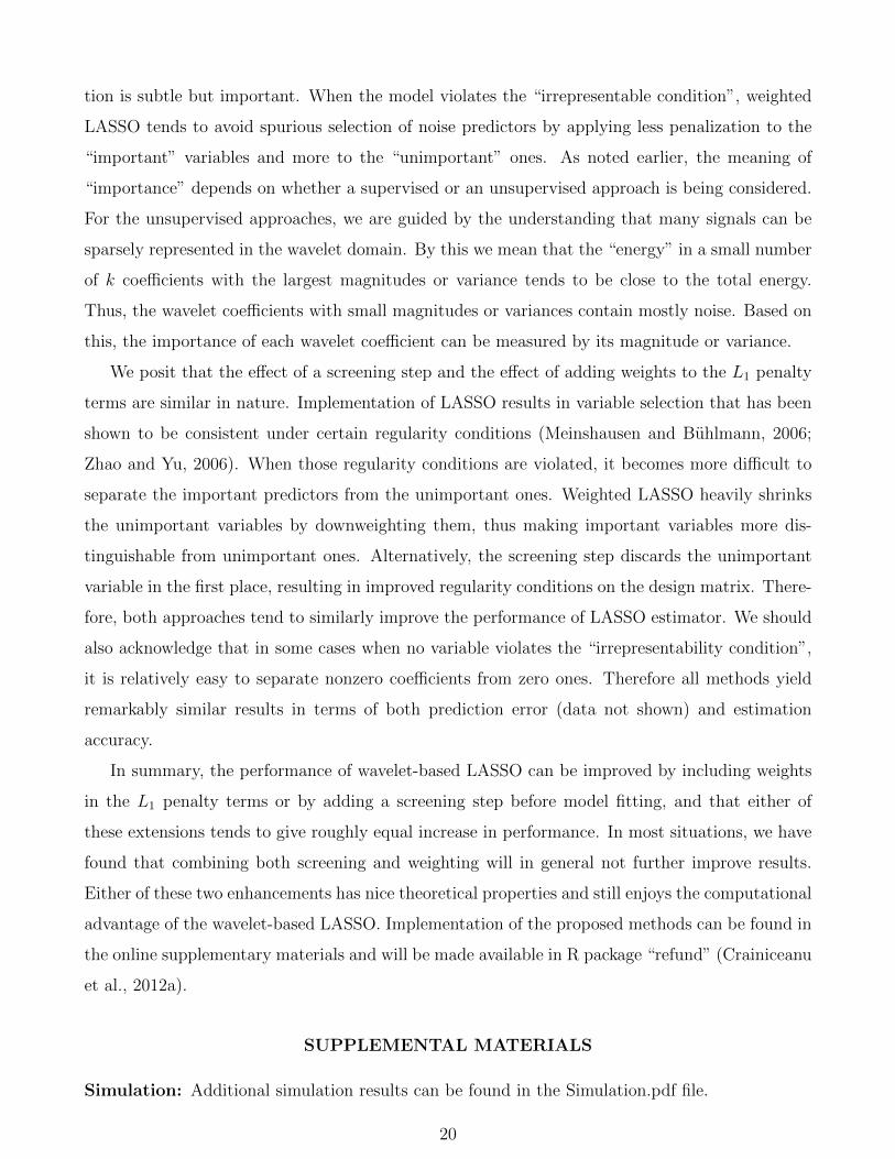
tion is subtle but important. When the model violates the “irrepresentable condition”, weighted
LASSO tends to avoid spurious selection of noise predictors by applying less penalization to the
“important” variables and more to the “unimportant” ones. As noted earlier, the meaning of
“importance” depends on whether a supervised or an unsupervised approach is being considered.
For the unsupervised approaches, we are guided by the understanding that many signals can be
sparsely represented in the wavelet domain. By this we mean that the “energy” in a small number
of k coefficients with the largest magnitudes or variance tends to be close to the total energy.
Thus, the wavelet coefficients with small magnitudes or variances contain mostly noise. Based on
this, the importance of each wavelet coefficient can be measured by its magnitude or variance.
We posit that the effect of a screening step and the effect of adding weights to the L1 penalty
terms are similar in nature. Implementation of LASSO results in variable selection that has been
shown to be consistent under certain regularity conditions (Meinshausen and Buhlmann, 2006;
Zhao and Yu, 2006). When those regularity conditions are violated, it becomes more difficult to
separate the important predictors from the unimportant ones. Weighted LASSO heavily shrinks
the unimportant variables by downweighting them, thus making important variables more dis-
tinguishable from unimportant ones. Alternatively, the screening step discards the unimportant
variable in the first place, resulting in improved regularity conditions on the design matrix. There-
fore, both approaches tend to similarly improve the performance of LASSO estimator. We should
also acknowledge that in some cases when no variable violates the “irrepresentability condition”,
it is relatively easy to separate nonzero coefficients from zero ones. Therefore all methods yield
remarkably similar results in terms of both prediction error (data not shown) and estimation
accuracy.
In summary, the performance of wavelet-based LASSO can be improved by including weights
in the L1 penalty terms or by adding a screening step before model fitting, and that either of
these extensions tends to give roughly equal increase in performance. In most situations, we have
found that combining both screening and weighting will in general not further improve results.
Either of these two enhancements has nice theoretical properties and still enjoys the computational
advantage of the wavelet-based LASSO. Implementation of the proposed methods can be found in
the online supplementary materials and will be made available in R package “refund” (Crainiceanu
et al., 2012a).
SUPPLEMENTAL MATERIALS
Simulation: Additional simulation results can be found in the Simulation.pdf file.
20

Appendix: The derivation of Theorem 1 and 2 can be found in the Appendix.pdf
supp.zip: The supp.zip file includes datasets used in the study and R code to perform the pro-
posed methods.
Acknowledgements
The authors thank Yongchao Ge, Philip T. Reiss, and Ciprian M Crainiceanu for insightful dis-
cussions. The authors would also like to thank the editor, the associate editor, and the refer-
ees for helpful comments. This work is partially supported by NIH grants 5R0EB009744 and
5R01MH099003 to R. Todd Ogden.
References
Abramovich F., Bailey T., and Sapatinas T.(2000). Wavelet analysis and its statistical
applications. The Statistician 49 1-29.
ADHD-200 Consortium (2012). The ADHD-200 Consortium: a model to advance the transla-
tional potential of neuroimaging in clinical neuroscience. Frontiers in Systems Neuroscience 6
62.
Amato U., Antoniadis A., and De Feis I. (2006). Dimension Reduction in Functional Re-
gression with Applications. Computational Statistics and Data Analysis 50 2422-2446.
Antoniadis A. and Sapatinas T. (2007). Estimation and inference in functional mixed-effects
models. Computational Statistics and Data Analysis 51 4793-4813.
Cai TT. and Hall P. (2006). Prediction in functional linear regression. Annals of Statistics 34
2159-2179.
Cardot, H., Ferraty, F. and Sarda, P. (2003). Spline Estimators for the Functional Linear
Model. Statistica Sinica 13 571-591.
Cardot, H., and Sarda, P. (2005). Estimation in generalized linear models for functional data
via penalized likelihood. Journal of Multivariate Analysis 92 24-41.
Crainiceanu, CM., Staicu, AM., and Di, CZ. (2009) Generalized Multilevel Functional Re-
gression. Journal of the American Statistical Association 104 15501561.
21

Crainiceanu, C., Reiss, P., Goldsmith, J., Huang, L., Huo, L., Scheipl, F., and Zhao,
Y. (2012). refund: Regression with Functional Data. R package version 0.1-6, URL http:
//CRAN.R-project.org/package=refund.
Crainiceanu, CM., Staicu, AM., Rayc, BS., and Punjabid, N. (2012) Bootstrap-based
inference on the difference in the means of two correlated functional processes. Statistics in
Medicine 31 32233240.
Crambes C. and Kneip A. and Sarda P. (2009). Smoothing Splines Estimators for Functional
Linear Regression. Annals of Statistics 37 35-72.
Delaigle A., Hall P., and Apanasovich T.V. (2009). Weighted Least Squares Methods for
Prediction in the Functional Linear Model. Electronic Journal of Statistics 3 865-885.
Donoho, D. and Johnstone, I. (1994). Ideal Spatial Adaptation via Wavelet Shrinkage.
Biometrika 81 425-455.
Donoho, D., Johnstone, I.,Kerkyacharian, G. and Picard, D. (1996). Density Estimation
By Wavelet Thresholding. The Annals of Statistics 24 508-539.
Fan, J. and Lv, J. (2008). Sure Independence Screening for Ultrahigh Dimensional Feature Space
(With Discussion). Journal of Royal Statistical Society Series B 70 849-911.
Fan, J. and Lv, J. (2010). A Selective Overview of Variable Selection in High Dimensional Feature
Space. Statistica Sinica 20 101-148.
Goldsmith, J., Crainiceanu, CM., Brian, Caffo. and Daniel, R. (2012). Longitudinal
Penalized Functional Regression for Cognitive Outcomes on Neuronal Tract Measurements.
Journal of Royal Statistical Society Series C 61 453469.
Goldsmith, J., Huang, L. and Crainiceanu, C. M. (2014). Smooth Scalar-on-Image Regres-
sion via Spatial Bayesian Variable Selection. Journal of Computational and Graphical Statistics
23 46-64.
Hall P. and Horowitz J. L. (2007). Methodology and Convergence Rates for Functional Linear
Regression. Annals of Statistics 35 70-91.
Huang, J., Ma, S. and Zhang, C.(2008). Adaptive Lasso for Sparse High-dimensional Regres-
sion Models. Statistica Sinica 18 1603-1618.
22

James, G.M.,, Wang, J., and Zhu, J. (2009). Functional Linear Regression That’s inter-
pretable. The Annals of Statistics 37 2083-2108.
Johnstone, I. and Lu, A. (2009). On Consistency and Sparsity for Principal Components
Analysis in High Dimensions. Journal of American Statistical Association 104 682-693.
Kalivas, J. H. (1997). Two Data Sets of Near-Infrared Spectra. Chemometrics and Intelligent
Laboratory Systems 37 255-259.
Lee, E. and Park, B. (2012). Sparse Estimation in Functional Linear Regression. Journal of
Multivariate Analysis 105 1-17.
Li, Y. and Hsing, T. (2007). On rates of convergence in functional linear regression. Journal of
Multivariate Analysis 98 1782-1804.
Malloy E. and Morris J. and Adar S. and Suh H. and Gold D. and Coull B. (2010).
Wavelet-based Functional Linear Mixed Models: an Application to Measurement Error corrected
Distributed Lag Models. Biostatistics 11 432-452.
Meinshausen, N. and Buhlmann, P. (2006). High Dimensional Graphs and Variable Selection
With the Lasso. The Annals of Statistics 34 1436-1462.
Meinshausen, N. and Buhlmann, P. (2010). Stability Selection (With Discussion). Journal of
Royal Statistical Society Series B 72 417-473.
Muller H. and Yao F. (2008) Functional Additive Models. Journal of the American Statistical
Association 103 1534-1544.
Nason, G. (2010). Wavethresh: Wavelets statistics and transforms. R package version 4.5.
Ogden, R.T. (1997). Essential Wavelets for Statistical Applications and Data Analysis.
Birkhauser, Boston
Reiss P. T. and Ogden R. T. (2007). Functional Principal Component Regression and Func-
tional Partial Least Squares. Journal of the American Statistical Association 102 984-996.
Reiss, P., Huo, L, Ogden, RT, Zhao, Y and Kelly, C (2014). Wavelet-Domain Methods for
Scalar-on-Image Regression. submitted
23

Shaw, P., Lerch, J., Greenstein, D, Sharp, W, Clasen, L., Evans, A., Giedd, J.,
Castellanos, FX. and Rapport, J. (2006). Longitudinal Mapping of Cortical Thickness and
Clinical Outcome in Children and Adolescents With Attention-Deficit/Hyperactivity Disorder.
Archives of General Psychiatry 63 540-549.
Tibshirani, R. (1996). Regression Shrinkage and Selection via the Lasso. Journal of Royal Sta-
tistical Society Series B 58 267-288.
Vidakovic, B. (1999). Statistical Modeling by Wavelets. Wiley, New York
Wang, X., Ray, S., and Mallick, B. (2007). Bayesian Curve Classification using wavelets.
Journal of the American Statistical Association 102 962-973.
Zhao, P. and Yu, B. (2006). On Model Selection Consistency of Lasso Journal of Machine
Learning Research 7 2541-2563.
Zhao, Y., Ogden, R.T and Reiss, P.T (2012). Wavelet-based LASSO in Functional Linear
Regression. Journal of Computational and Graphical Statistics 21 600-617.
Zhu, H., Brown, P.J and Morris, J.S (2012). Robust Classification of Functional and Quan-
titative Image Data Using Functional Mixed Models. Biometrics 68 1260-1268.
Zou, H. and Hastie, T. (2005). Regularization and variable selection via the elastic net. Journal
of Royal Statistical Society Series B 67 301-320.
Zou, H. (2006). The Adaptive Lasso and Its Oracle Properties. Journal of the American Statistical
Association 101 1418-1428.
Appendix A Proof of Theorems
Proof of Theorem 1
Proof. Let βSnbe a kn × 1 vector in which Sn entries are nonzero, θ = {θj, j = 1, . . . , kn}
be the estimated sample wavelet coefficient magnitude, and ρkn be the smallest eigenvalue of
Σkn = 1nZT
knZkn . Without loss of generality, we assume the first Sn entries in βSnare nonzero,
24

and assume columns of Zkn are standardized such that each column has mean of 0 and standard
deviation of 1, and the first Sn elements of θ are nonzero. By Parseval’s theorem, we have
||ηn − η||2L2 = ‖ βkn − βSn‖2 +
kn∑j=Sn+1
β2j +
Nn∑j=kn+1
β2j +
∞∑j=Nn+1
β2j . (A.1)
The first term on right hand side of equation (A.1) stands for model estimation error, the second
term is due to thresholding error, the third term is due to screening error, and the fourth term
is due to finite sampling error which depends on how densely we sample the functional predictor.
By assumption (a4) and Theorem 9.5 of ?,
∞∑j=Nn+1
β2j = o(N−2qn ). (A.2)
By assumption (a5) and Theorem 9.10 of ?,
kn∑j=Sn+1
β2j +
Nn∑j=kn+1
β2j =
Nn∑j=Sn+1
β2j = o(S1−2/r
n ). (A.3)
We show the convergence rate of ‖ βkn−βSn‖2 below. Let l(β) = 1/n||Y−ZT
knβ||2+∑kn
j=1 λnθ−1j |βj|,
δ = ||βkn − βSn||, and βkn − βSn
= δu with ||u|| = 1. Given equation (4), we have
l(βkn)− l(βSn) = −2δn−1ε∗TZT
knu + δ2n−1uTZTknZknu +
kn∑j=1
λnθ−1j (|βj| − |βj|) ≤ 0. (A.4)
We know∑kn
j=1 λnθ−1j (|βj| − |βj|) ≥
∑j∈Hn
λnθ−1j (|βj| − |βj|). By reverse triangle inequality and
Cauchy-Schwarz inequality, we have∑j∈Hn
λnθ−1j (|βj| − |βj|) ≥ −
∑j∈Hn
λnθ−1j (|βj − βj|) ≥ −δ
√∑j∈Hn
(λnθ−1j )2. (A.5)
Combine (A.4) and (A.5), we have
δρkn ≤ δuTΣknu ≤ 2||n−1ZTHnε∗||+
√∑j∈Hn
(λnθ−1j )2. (A.6)
We next show the convergence rate of ||n−1ZTknε∗|| in equation (A.6). Given equation (4), a
constant C, and ξ2i = (Nn∑
i=kn+1
zijβj)2,
E(||n−1/2ZTknε∗||2) = E(n−1εTZT
knZknε) + n−1ξTZTknZknξ
≤ σ2tr(Σkn) + C/n
n∑i=1
ξ2i
≤ σ2kn + 1/nn∑
i=1
(Nn∑
j=kn+1
z2ij
)(Nn∑
j=kn+1
β2j
)
25

By assumption (a4), E(||n−1/2ZTknε∗||2) = O(kn) + o(k
1−2/rn ). By Markov’s inequality,
||n−1ZTHnε∗|| = Op((kn/n)1/2) + op(k
1/2−1/rn /
√n). (A.7)
By assumption (a2), we have√ ∑
j∈Hn
(λnθ−1j )2 = op(n
−1/2). Combining this with (A.7) and (A.6),
we have
δ = ‖ βkn − βSn‖ = Op
(k1/2n
n1/2ρkn
). (A.8)
By (A.2), (A.3), and (A.8), this implies
‖ ηn − η‖ 2L2 = Op
(knnρ2kn
)+ o(k1−2/rn ) + o(N−2qn )
Proof of Theorem 2
Proof. Following Johnstone and Lu (2009), we assume, without loss of generality, that wavelet
coefficient population magnitude θ1 ≥ θ2 ≥ · · · ≥ θN > 0. We also assume the coefficient of
variation for each wavelet coefficient is bounded by a constant C0 (i.e., Ch = σh/θh, 0 < Ch <
C1, h = 1, 2, . . . , N), where σ2h, h = 1, . . . , N is the population variance of wavelet coefficient.
Let γn be a suitably chosen small positive number, and d be a suitably chosen constant. Let
zh ∼ N(µh, σ2h), θh = |µh| ∀h, and Z ∼ N(0, 1). For any fixed constant t and l ∈M ,
θh ≤ t for h ≥ k, h 6= l and θl ≥ t⇒ θl ≥ θ(k).
If we let t = θk + γn and θl ≥ d× t with d > 1, we have
P (θl < θ(k)) ≤∑h≥k
P (θh > t) + P (θl < t) =∑h≥k
{P
(Z >
√n(t− θh)
σh
)+ P
(Z <
√n(−t− θh)
σh
)}+ P
(√n(−t− θl)
σl< Z <
√n(t− θl)σl
)=∑h≥k
{P
(Z >
√n(t/θh − 1)
σh/θh
)+ P
(Z >
√n(t/θh + 1)
σh/θh
)}+ P
(Z >
√n(1− t/θl)σl/θl
)− P
(Z >
√n(1 + t/θl)
σl/θl
)≤∑h≥k
{P
(Z >
√n(γn/θk)
C0
)+ P
(Z >
√n(γn/θk + 2)
C0
)}+ P
(Z >
√n(1− 1/d)
C0
)= (N − k + 1) Φ
(−√nγn/θkC0
)+ (N − k + 1) Φ
(−√n(2 + γn/θk)
C0
)+ Φ
(√n(1/d− 1)
C0
)26

The bound P (FE) ≤ (N − k + 1) Φ(−√n
C0b
)+ (N − k + 1) Φ
(−√n(2b+1)C0b
)+ Φ
(√n(1−d)dC0
)follows
from γn =√log(n)/n, θk = bγn with b > 0, and a suitably chosen constant d > 1.
27

Fig
ure
1:P
redic
tion
per
form
ance
:M
ean
Abso
lute
Err
orbas
edon
200
sim
ula
ted
dat
aset
s(R
ow1-
Row
3:R
2=
0.9,
0.5,
0.2;
Col
um
n1:
No
scre
enin
g,C
olum
n2:
Scr
eenin
gby
vari
ance
,C
olum
n3:
Scr
eenin
gby
mag
nit
ude
ofw
avel
etco
effici
ents
,C
olum
n4:
Scr
eenin
gby
mag
nit
udes
ofco
rrel
atio
nco
effici
ents
,C
olum
n5:
Scr
eenin
gby
stab
ilit
yse
lcti
on).
Hor
izon
tal
line
stan
ds
for
sam
ple
mea
nfr
omW
m
wit
hm
agnit
ude
scre
enin
gm
ethod
28

Fig
ure
2:E
stim
atio
np
erfo
rman
ce:
Mea
nIn
tegr
ate
Squar
edE
rror
bas
edon
200
sim
ula
ted
dat
aset
s(R
ow1-
Row
3:R
2=
0.9,
0.5,
0.2;
Col
um
n1:
No
scre
enin
g,C
olum
n2:
Scr
eenin
gby
vari
ance
,C
olum
n3:
Scr
eenin
gby
mag
nit
ude
ofw
avel
etco
effici
ents
,C
olum
n4:
Scr
eenin
gby
mag
nit
udes
ofco
rrel
atio
nco
effici
ents
,C
olum
n5:
Scr
eenin
gby
stab
ilit
yse
lcti
on).
Hor
izon
tal
line
stan
ds
for
sam
ple
mea
n
from
Wm
wit
hm
agnit
ude
scre
enin
gm
ethod
29

Figure 3: Estimated mean and standard deviation functions of LASSO and weighted LASSO with
different weights at R2 = 0.9 based on 200 simulated datasets. Y axis ranges from 0 to 55 for
LASSO, and from 0 to 6 for others.
30

Figure 4: Estimated mean and standard deviation functions of LASSO with different screening
strategies at R2 = 0.9 based on 200 simulated datasets
31

Figure 5: The wheat data: Estimated coefficient function with their corresponding pointwise
(light gray) and joint (dark extensions) confidence intervals (Rows: 1-2) and permutation tests to
assessing statistical significance of the relationship (Rows: 3-4).
32

Fig
ure
6:th
eA
DH
Ddat
a:R
ow1:
Est
imat
edco
effici
ent
funct
ion;
Row
2:co
rres
pon
din
gim
ages
indic
atin
gre
gion
sw
ith
stat
isti
cal
sign
ifica
nce
ofth
ere
lati
onsh
ipbas
edon
95%
poi
ntw
ise
confiden
cein
terv
als;
Row
3:O
bse
rved
R2
(hor
izon
tal
line)
and
per
mute
dR
2
(cir
cles
)fo
ras
sess
ing
stat
isti
cal
sign
ifica
nce
ofth
ere
lati
onsh
ip
33