WAVEGUIDE BAND-PASS FILTERS AT KU BAND

FOR HIGH POWER SATELLITE COMMUNICATIONS

Krishna Rao (krishprasads@gmail.com)

I. INTRODUCTION

This technical report is to explain the design of a waveguide bandpass operating in the Ku band, intended

for handling high power, for satellite communication applications. Ku band operates from 12 – 18 GHz,

predominantly used in satellite television applications. High power transmitters require filters to suppress

side bands, at the same time handle such high power and be less lossy in the passband.

II. REQUIREMENTS

The waveguide is expected to operate in at 13.45 GHz center frequency (Ku band) with a bandwidth of

10%. At and beyond the 10% in the frequency scale, the waveguides are expected to suppress signals by

at least 15dB. The bandpass filter can be implemented using symmetric or asymmetric irises or inductive

posts. Passband ripple has to be designed for as minimum as possible.

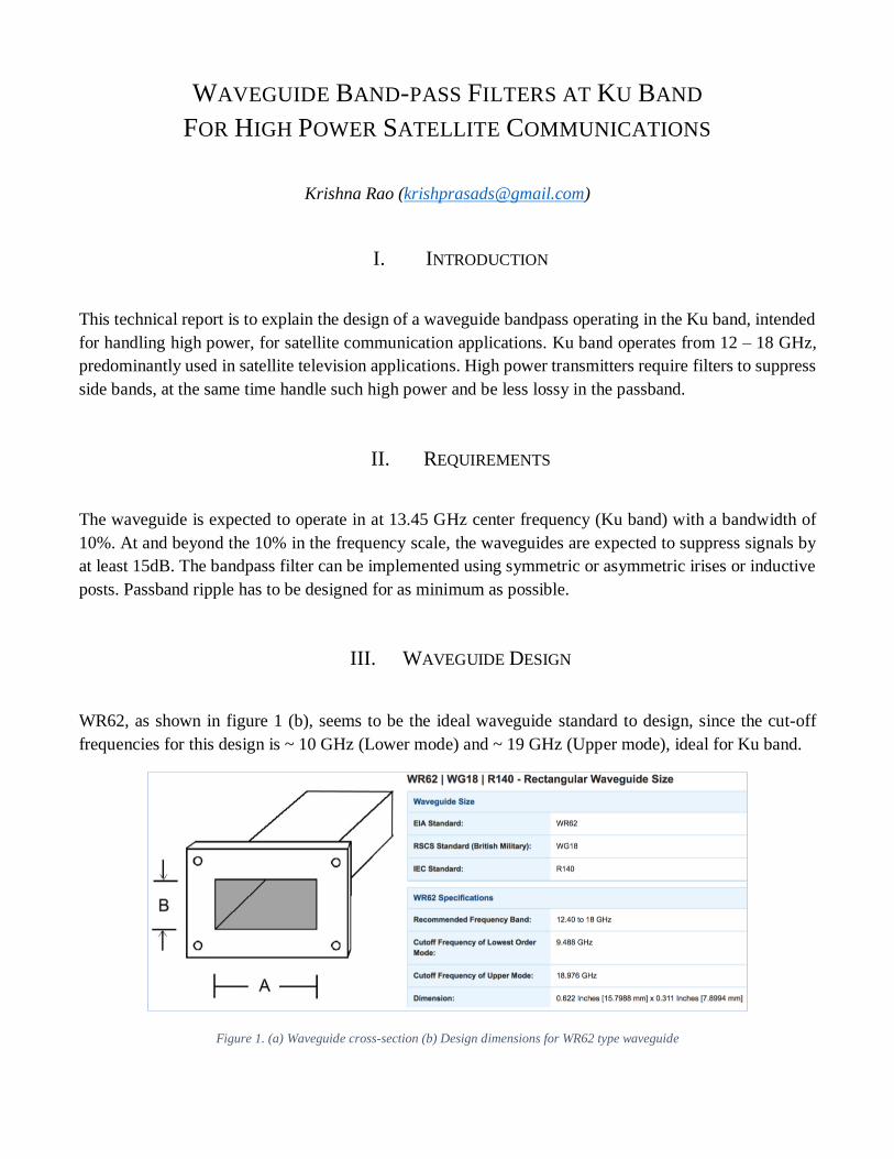
III. WAVEGUIDE DESIGN

WR62, as shown in figure 1 (b), seems to be the ideal waveguide standard to design, since the cut-off

frequencies for this design is ~ 10 GHz (Lower mode) and ~ 19 GHz (Upper mode), ideal for Ku band.

Figure 1. (a) Waveguide cross-section (b) Design dimensions for WR62 type waveguide

With the width (A) and the height (B) known of the waveguide type known, the waveguide is modeled on

CST with an assumed length. On the either ends of the modeled waveguide, ‘waveguide ports’ are created,

and an S-parameter simulation in the time domain is kicked off, with improved time domain meshing done

manually, if necessary.

Figure 2. (Left) Plain waveguide with dimensions (Right) Waveguide with ports

IV. WAVEGUIDE BAND-PASS FILTER DESIGN

In this report, band pass filter is implemented in the waveguide using symmetric irises. For a rejection of

15dB at 18GHz, as per figure 3, the filter order to be selected is N = 10. But, in order to keep the design

simple, a filter order of N = 5 is assumed.

Figure 3. Chebysheff filter parameters for 0.01dB ripple filter, courtesy of Altanta RF (atlantarf.com)

Once the filter order is determined, the next step is to get the filter parameter and type. Chebyshev filter

of order 5 with passband ripple of 0.01dB is selected for the design, whose filter coefficients are given

below.

Figure 4. Chebysheff filter element values for 0.01dB ripple for different filter orders, courtesy of RF Cafe (rfcafe.com)

To design symmetric irises, the dimensions – namely the iris width and the spacing between them have to

be determined. A simplified cross section of the desired band-pass filter wave guide is seen below.

Figure 5. Symmetric iris band-pass waveguide filter cross section from 'Electronic Filter Simulation & Design' by G. Bianchi & R.

Sorrentino pp. 544

From figure 5, it can be understood that the iris opening dimensions are dependent on susceptance ‘B’,

and the separation of the iris are dependent on electrical length θi. An image explaining the derivation of

these results can be found in the Appendix A, and more information can be found from the references.

The exact design equations involving susceptance and the electrical lengths can be found below:

1. The iris opening dimension ‘d’ can be calculated from susceptance as shown:

Figure 6. Formula for waveguide iris design, from 'Electronic Filter Simulation & Design' by G. Bianchi & R. Sorrentino pp. 536

To calculate B, the following equations are used:

K/Z0 values are given by:

where gi values are the highlighted Chebyshev filter coefficients from Table 1, where w is given

by:

g1, g2 are guide wavelengths at the band edges. g0 is given by

To compute these values, a MATLAB code is written, as seen in Appendix B, and the following

table of results, is generated.

Figure 7. Waveguide filter Susceptance and Electrical lengths computed from MATLAB

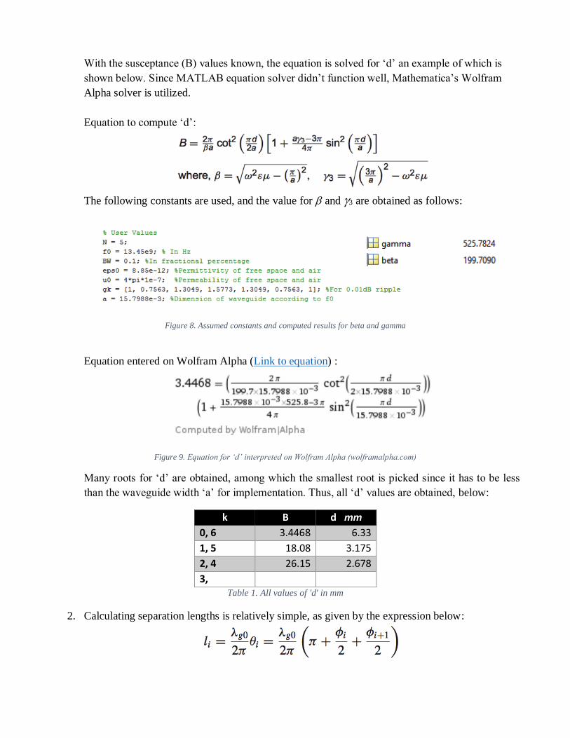
With the susceptance (B) values known, the equation is solved for ‘d’ an example of which is

shown below. Since MATLAB equation solver didn’t function well, Mathematica’s Wolfram

Alpha solver is utilized.

Equation to compute ‘d’:

The following constants are used, and the value for and 3 are obtained as follows:

Figure 8. Assumed constants and computed results for beta and gamma

Equation entered on Wolfram Alpha (Link to equation) :

Figure 9. Equation for ‘d’ interpreted on Wolfram Alpha (wolframalpha.com)

Many roots for ‘d’ are obtained, among which the smallest root is picked since it has to be less

than the waveguide width ‘a’ for implementation. Thus, all ‘d’ values are obtained, below:

k B d mm

0, 6 3.4468 6.33

1, 5 18.08 3.175

2, 4 26.15 2.678

3,

Table 1. All values of 'd' in mm

2. Calculating separation lengths is relatively simple, as given by the expression below:

Separation lengths are computed in MATLAB and the results are below:

Figure 10. Computed values of section lengths on MATLAB

Since both ‘d’ and ‘l’ have been computed, the irises are now modeled inside our waveguide from figure

2, as seen in figure 11. A buffer length of ~ 4mm is also added at the front and the back of the waveguide

for ease of manufacturability.

Figure 11. Modeled iris band-pass waveguide filter based on dimensions 'd' and 'l'

Necessary field monitors are added and the waveguide is manually meshed thoroughly. All edges

highlighted in green are meshed accurately, which generates a total mesh count of 731880 cells.

Figure 12. Mesh view of the modeled waveguide filter

Time domain simulation is then kicked off, which runs for about an hour.

V. RESULTS

1. Return Loss and Insertion Loss

Results show that the center frequency has moved significantly, to 16.43 GHz, from the designed

frequency of 13.45 GHz. Additionally, the passband ripple is seen to be around 0.5 dB, although

designed only for 0.01dB.

Figure 13. Insertion loss plot of the waveguide bandpass filter

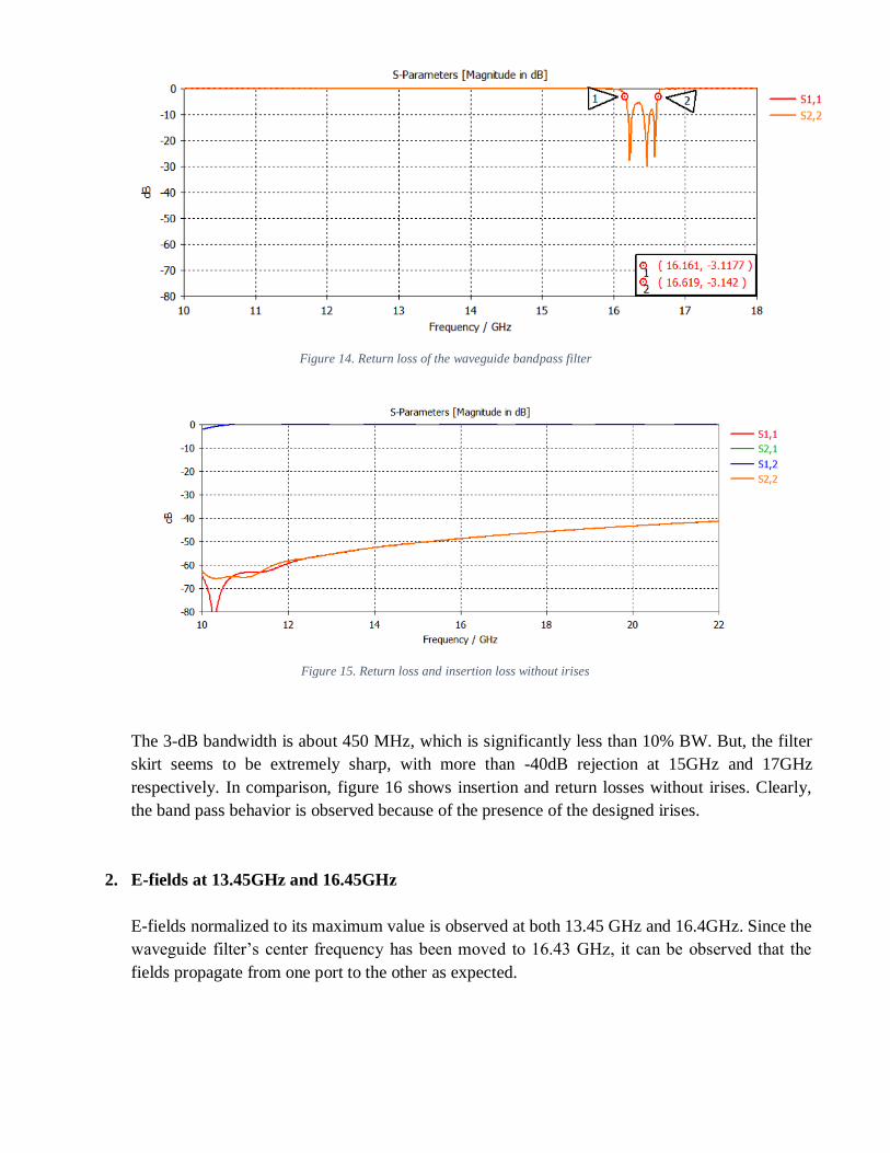
Figure 14. Return loss of the waveguide bandpass filter

Figure 15. Return loss and insertion loss without irises

The 3-dB bandwidth is about 450 MHz, which is significantly less than 10% BW. But, the filter

skirt seems to be extremely sharp, with more than -40dB rejection at 15GHz and 17GHz

respectively. In comparison, figure 16 shows insertion and return losses without irises. Clearly,

the band pass behavior is observed because of the presence of the designed irises.

2. E-fields at 13.45GHz and 16.45GHz

E-fields normalized to its maximum value is observed at both 13.45 GHz and 16.4GHz. Since the

waveguide filter’s center frequency has been moved to 16.43 GHz, it can be observed that the

fields propagate from one port to the other as expected.

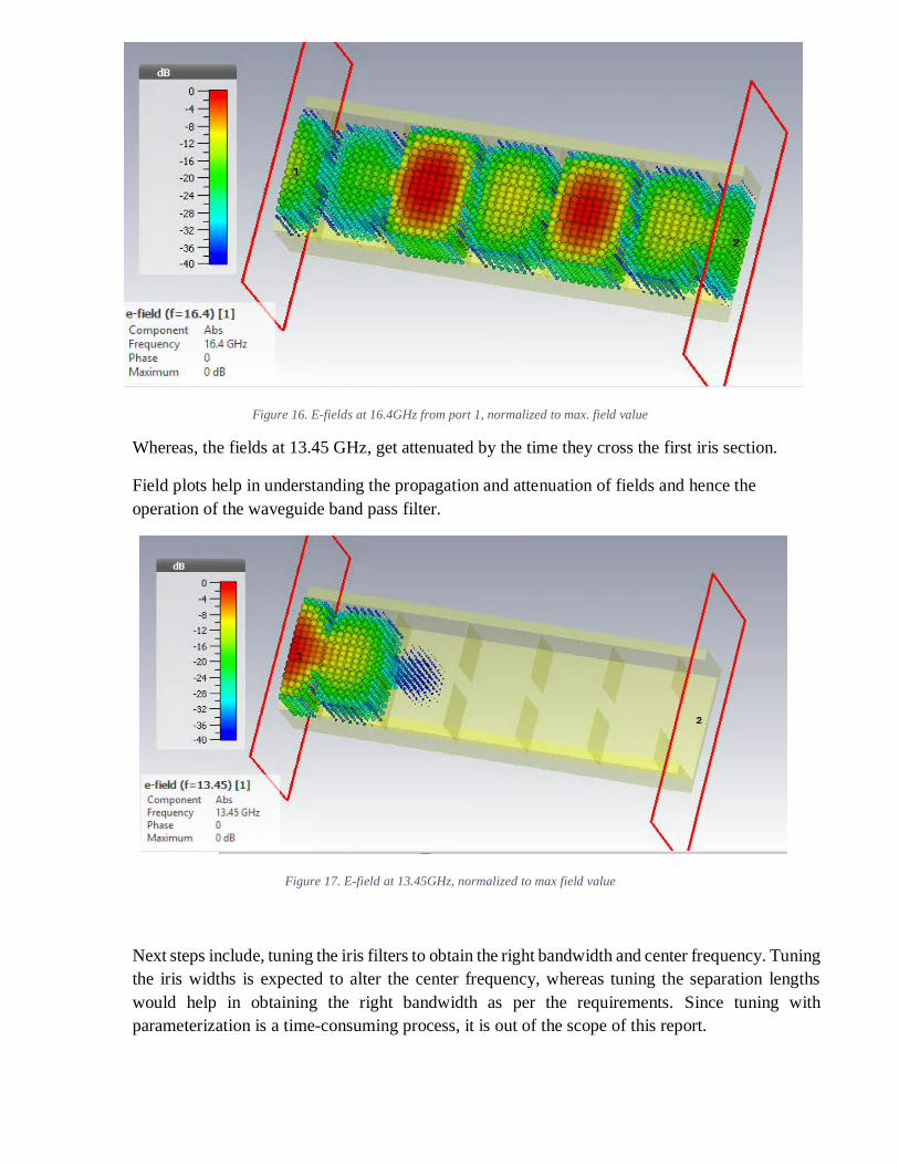
Figure 16. E-fields at 16.4GHz from port 1, normalized to max. field value

Whereas, the fields at 13.45 GHz, get attenuated by the time they cross the first iris section.

Field plots help in understanding the propagation and attenuation of fields and hence the

operation of the waveguide band pass filter.

Figure 17. E-field at 13.45GHz, normalized to max field value

Next steps include, tuning the iris filters to obtain the right bandwidth and center frequency. Tuning

the iris widths is expected to alter the center frequency, whereas tuning the separation lengths

would help in obtaining the right bandwidth as per the requirements. Since tuning with

parameterization is a time-consuming process, it is out of the scope of this report.

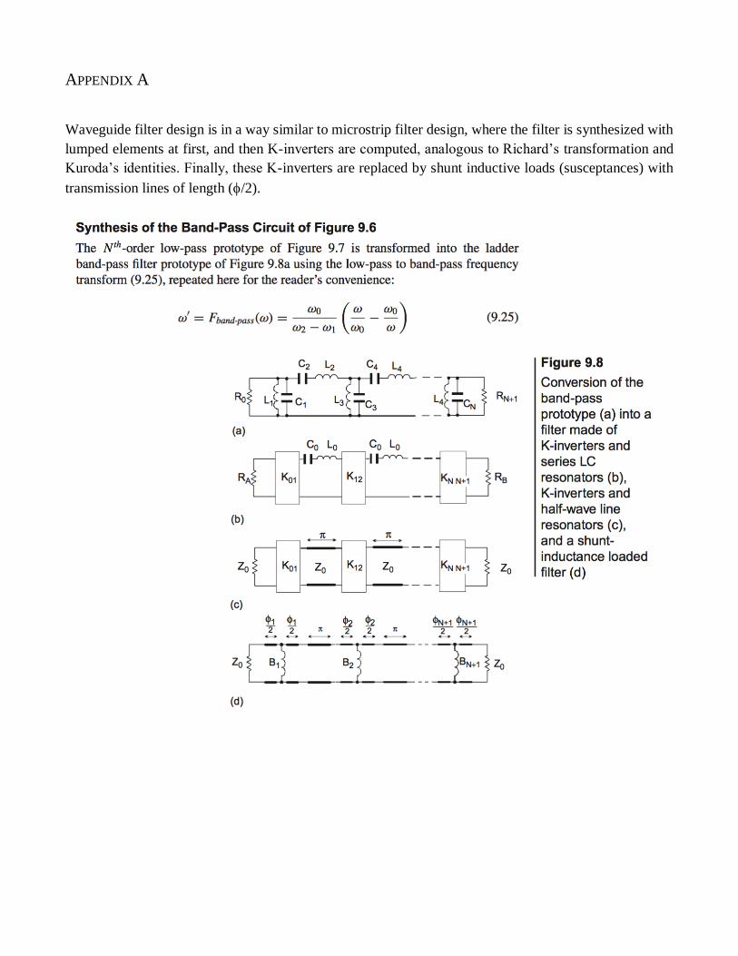
APPENDIX A

Waveguide filter design is in a way similar to microstrip filter design, where the filter is synthesized with

lumped elements at first, and then K-inverters are computed, analogous to Richard’s transformation and

Kuroda’s identities. Finally, these K-inverters are replaced by shunt inductive loads (susceptances) with

transmission lines of length (/2).

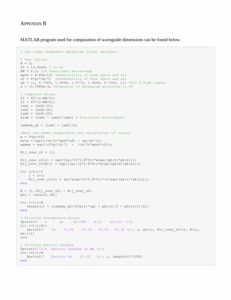
APPENDIX B

MATLAB program used for computation of waveguide dimensions can be found below.

% 5th order Chebyshev waveguide filter designer

% User Values

N = 5;

f0 = 13.45e9; % In Hz

BW = 0.1; %In fractional percentage

eps0 = 8.85e-12; %Permittivity of free space and air

u0 = 4*pi*1e-7; %Permeability of free space and air

gk = [1, 0.7563, 1.3049, 1.5773, 1.3049, 0.7563, 1]; %For 0.01dB ripple

a = 15.7988e-3; %Dimension of waveguide according to f0

% Computed values

f1 = f0*(1-BW/2);

f2 = f0*(1+BW/2);

lam1 = (3e8)/f1;

lam2 = (3e8)/f2;

lam0 = (3e8)/f0;

wlam = (lam1 - lam2)/lam0; % Fractional wavelengths

lambda_g0 = (lam1 + lam2)/2;

%Beta and Gamma computation for calculating 'd' values

w = 2*pi*f0;

beta = sqrt(((w^2)*eps0*u0) - (pi/a)^2);

gamma = sqrt((3*pi/a)^2 - ((w^2)*eps0*u0));

Kij_over_z0 = [];

Kij_over_z0(1) = sqrt((pi/(2*2.875))*wlam/(gk(1)*gk(2)));

Kij_over_z0(N+1) = sqrt((pi/(2*2.875))*wlam/(gk(5)*gk(6)));

for i=2:1:5

j = i+1;

Kij_over_z0(i) = (pi*wlam/(2*2.875))*(1/sqrt(gk(i)*gk(j)));

end

B = (1./Kij_over_z0) - Kij_over_z0;

phi = -atan(2./B);

for i=1:1:N

length(i) = (lambda_g0/(2*pi))*(pi + phi(i)/2 + phi(i+1)/2);

end

% Printing Susceptance values

fprintf(' k gk Kij/B0 B(j) phi(j) \n')

for i=1:1:N+1

fprintf(' %d %3.3f %3.3f %3.3f %3.3f \n', i, gk(i), Kij_over_z0(i), B(i),

phi(i))

end

% Printing Section lengths

fprintf('\n\n Section Lengths in mm \n')

for i=1:1:N

fprintf(' Section %d %3.3f \n', i, length(i)*1000)

end

REFERENCES

1. Giovanni Bianchi, Roberto Sorrentino, “Electronic Filter Simulation & Design”

2. David Pozar, “Microwave Engineering”, 4th Edition