Waveform Modeling and Comparisons with Ground Truth Events

 

David Norris

BBN Technologies

1300 N. 17th Street

Arlington, VA 22209

dnorris@bbn.com

703-284-1348

14 Nov 2007

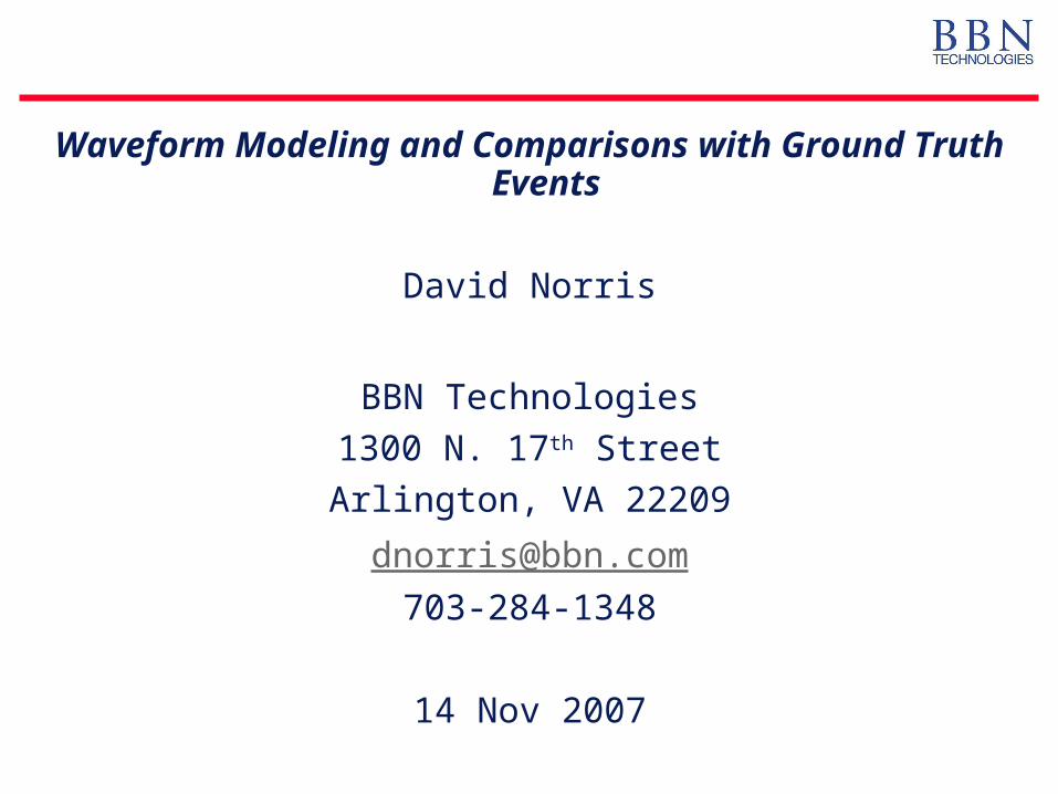
Motivation

• Quantify terrain effects on predicted travel times and waveform parameters

• Provide seamless integration between terrain and atmospheric specifications

• Improve overall propagation modeling capabilities and suite of tools that can be utilized by analysts and researchers

InfraMAP – Infrasonic Modeling of Atmospheric Propagation

Terrain Modeling Approaches

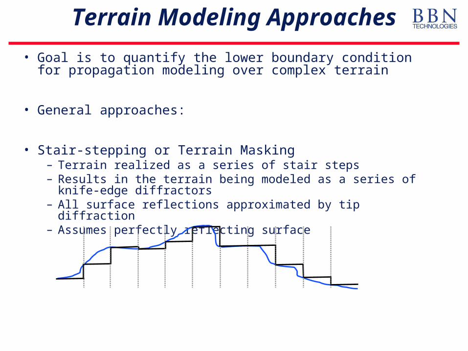
• Goal is to quantify the lower boundary condition for propagation modeling over complex terrain

• General approaches:

• Stair-stepping or Terrain Masking– Terrain realized as a series of stair steps– Results in the terrain being modeled as a series of knife-edge diffractors– All surface reflections approximated by tip diffraction– Assumes perfectly reflecting surface

Terrain Modeling Approaches (Cont.)

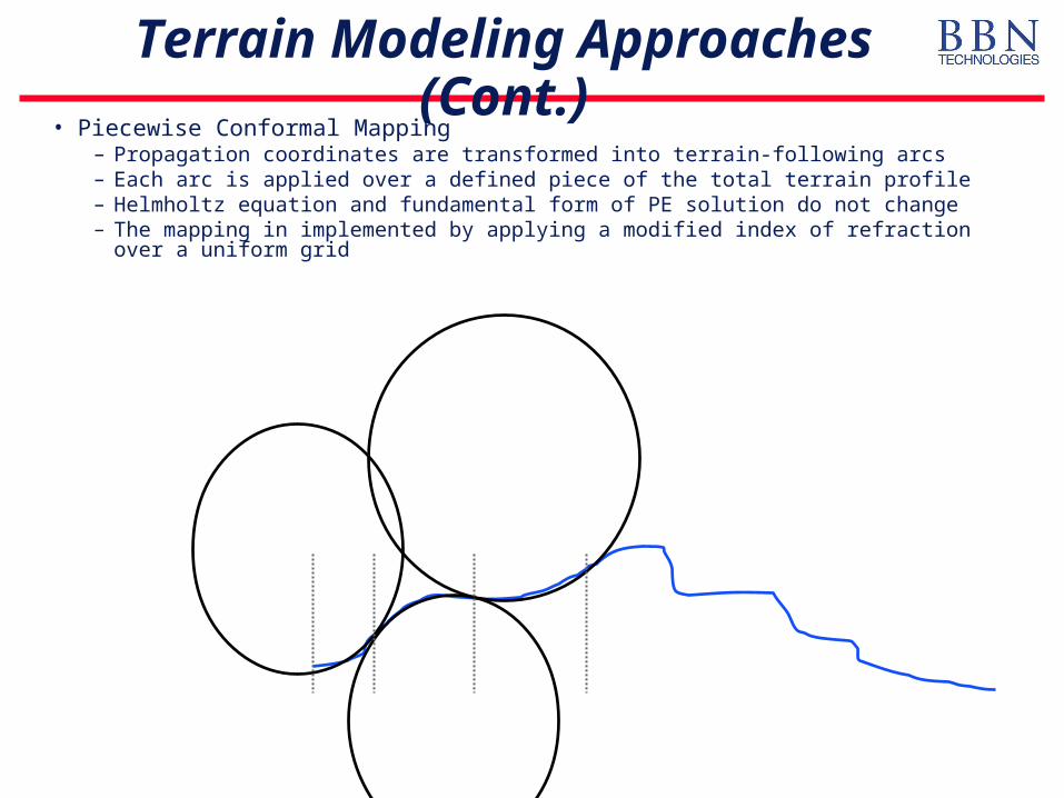
• Piecewise Conformal Mapping– Propagation coordinates are transformed into terrain-following arcs– Each arc is applied over a defined piece of the total terrain profile– Helmholtz equation and fundamental form of PE solution do not change– The mapping in implemented by applying a modified index of refraction

over a uniform grid

Terrain Modeling Approaches (Cont.)

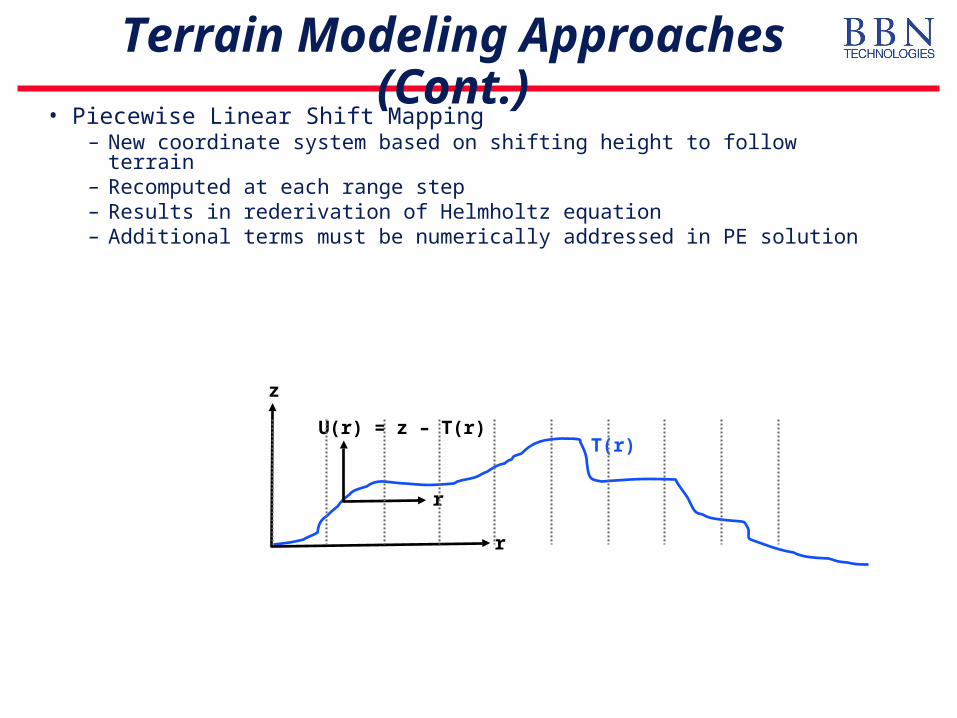
• Piecewise Linear Shift Mapping– New coordinate system based on shifting height to follow terrain– Recomputed at each range step – Results in rederivation of Helmholtz equation– Additional terms must be numerically addressed in PE solution

r

z

T(r)

r

U(r) = z – T(r)

Terrain Masking Approach

Range (km)

He

igh

t (km

)

PE with absorption: Amplitude Field (dB re 1 km)

0 50 1000

5

10

15

20

-100

-80

-60

-40

-20

0

Range (km)

He

igh

t (km

)

PE with absorption: Amplitude Field (dB re 1 km)

0 50 1000

5

10

15

20

-100

-80

-60

-40

-20

0

Range (km)

He

igh

t (km

)

PE with absorption: Amplitude Field (dB re 1 km)

0 50 1000

5

10

15

20

-100

-80

-60

-40

-20

0

Range (km)

He

igh

t (km

)

PE with absorption: Amplitude Field (dB re 1 km)

0 50 1000

5

10

15

20

-100

-80

-60

-40

-20

0

Range (km)

He

igh

t (km

)

PE with absorption: Amplitude Field (dB re 1 km)

0 50 1000

5

10

15

20

-100

-80

-60

-40

-20

0

Range (km)

He

igh

t (km

)

PE with absorption: Amplitude Field (dB re 1 km)

0 50 1000

5

10

15

20

-100

-80

-60

-40

-20

0

Mt. Everest

Mt. Fuji

Mt. Everest

Mt. Fuji

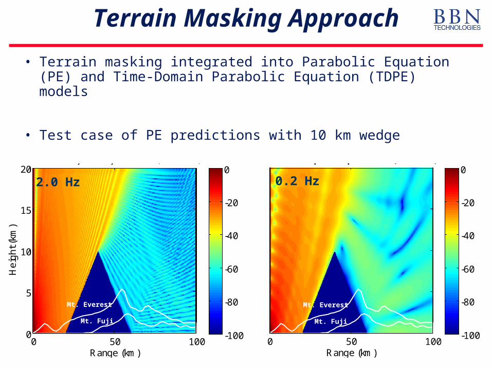
• Terrain masking integrated into Parabolic Equation (PE) and Time-Domain Parabolic Equation (TDPE) models

• Test case of PE predictions with 10 km wedge

2.0 Hz 0.2 Hz

Hypothetical Scenario

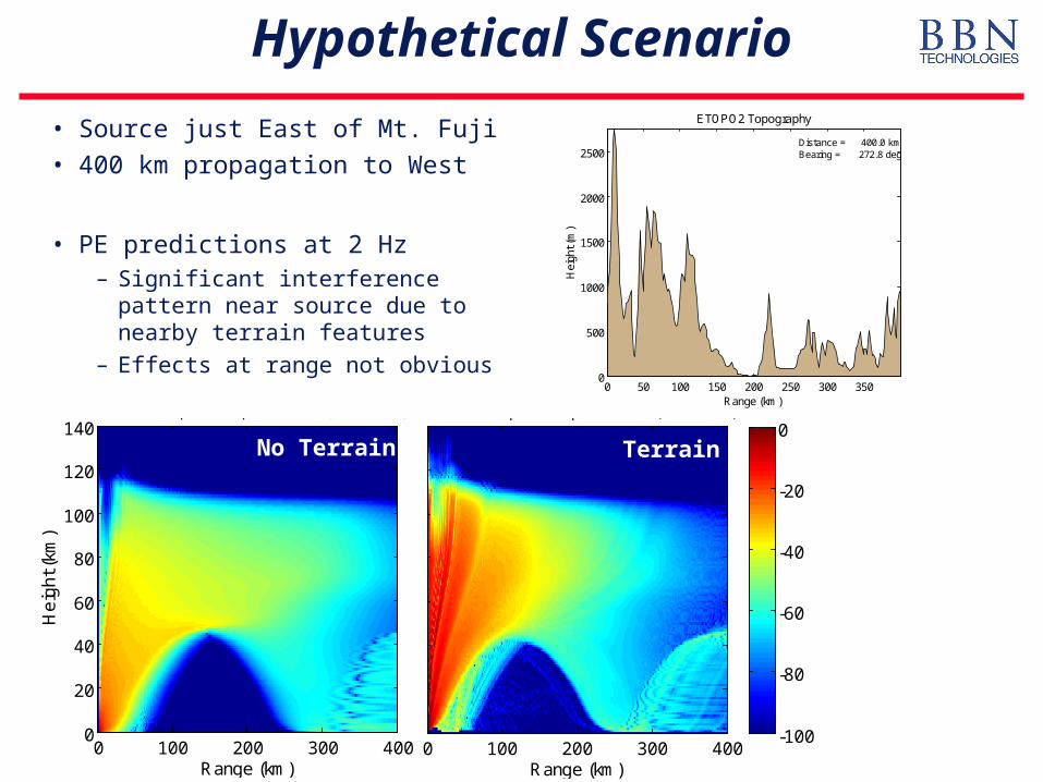
• Source just East of Mt. Fuji

• 400 km propagation to West

• PE predictions at 2 Hz– Significant interference pattern

near source due to nearby terrain features

– Effects at range not obvious 0 50 100 150 200 250 300 3500

500

1000

1500

2000

2500

Range (km)

Hei

ght (

m)

ETOPO2 Topography

Distance = 400.0 kmBearing = 272.8 deg

Range (km)

He

igh

t (km

)

PE with absorption: Amplitude Field (dB re 1 km)

0 100 200 300 4000

20

40

60

80

100

120

140

-100

-80

-60

-40

-20

0

Range (km)

He

igh

t (km

)

PE with absorption: Amplitude Field (dB re 1 km)

0 100 200 300 4000

20

40

60

80

100

120

140

-100

-80

-60

-40

-20

0No Terrain Terrain

Hypothetical Scenario (cont.)

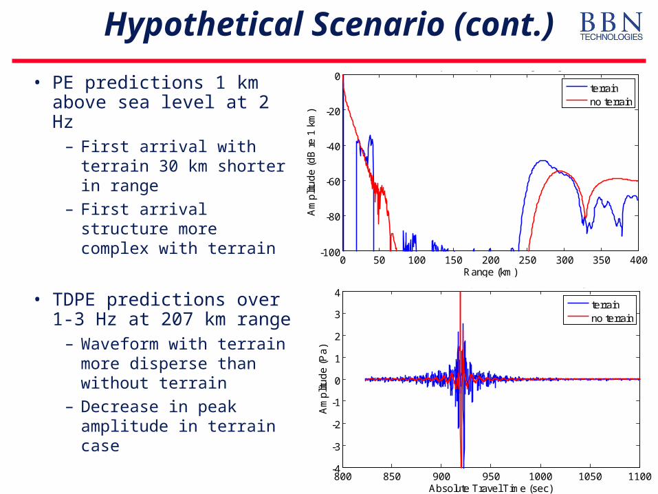
• PE predictions 1 km above sea level at 2 Hz

– First arrival with terrain 30 km shorter in range

– First arrival structure more complex with terrain

• TDPE predictions over 1-3 Hz at 207 km range

– Waveform with terrain more disperse than without terrain

– Decrease in peak amplitude in terrain case

Terrain

0 50 100 150 200 250 300 350 400-100

-80

-60

-40

-20

0

Range (km)

Am

plit

ud

e (

dB

re

1 k

m)

PE with absorption: Amplitude vs. Range, Height: 1 km

terrainno terrain

800 850 900 950 1000 1050 1100-4

-3

-2

-1

0

1

2

3

4

Absolute Travel Time (sec)

Am

plit

ud

e (

Pa

)

Time-domain PE with absorption: Amplitude vs. Time, Height: 1 km

terrainno terrain

Henderson Event

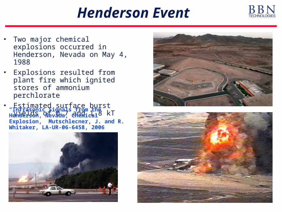
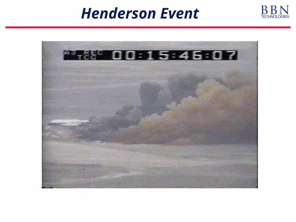
• Two major chemical explosions occurred in Henderson, Nevada on May 4, 1988

• Explosions resulted from plant fire which ignited stores of ammonium perchlorate

• Estimated surface burst yields of 0.7 and 1.8 kT

“Infrasonic Signals from the Henderson, Nevada, Chemical Explosion,” Mutschlecner, J. and R. Whitaker, LA-UR-06-6458, 2006

Henderson Event

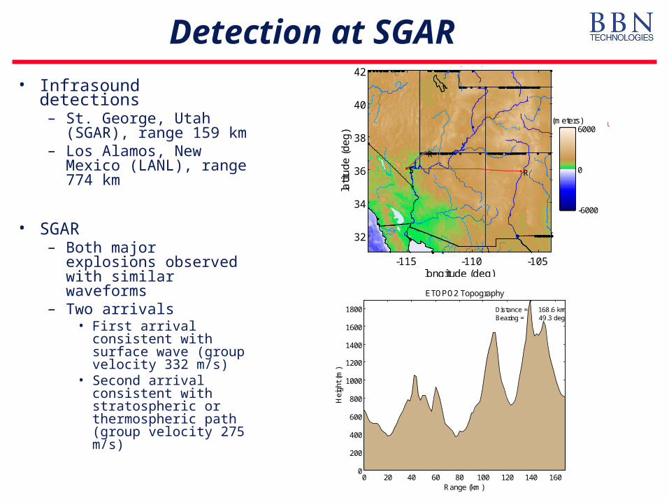
Detection at SGAR

• Infrasound detections– St. George, Utah

(SGAR), range 159 km– Los Alamos, New

Mexico (LANL), range 774 km

• SGAR– Both major explosions

observed with similar waveforms

– Two arrivals• First arrival consistent

with surface wave (group velocity 332 m/s)

• Second arrival consistent with stratospheric or thermospheric path (group velocity 275 m/s)

(meters)

-6000

0

6000

longitude (deg)

latit

ud

e (

de

g)

ETOPO2: Topography (meters)

UNITED STATES

S R S

R

-115 -110 -105

32

34

36

38

40

42

0 20 40 60 80 100 120 140 1600

200

400

600

800

1000

1200

1400

1600

1800

Range (km)

Hei

ght (

m)

ETOPO2 Topography

Distance = 168.6 kmBearing = 49.3 deg

Range (km)

He

igh

t (km

)

0 50 100 1500

20

40

60

80

100

120

140

-100

-80

-60

-40

-20

0

Range (km)

He

igh

t (km

)

0 50 100 1500

20

40

60

80

100

120

140

-100

-80

-60

-40

-20

0No Terrain Terrain

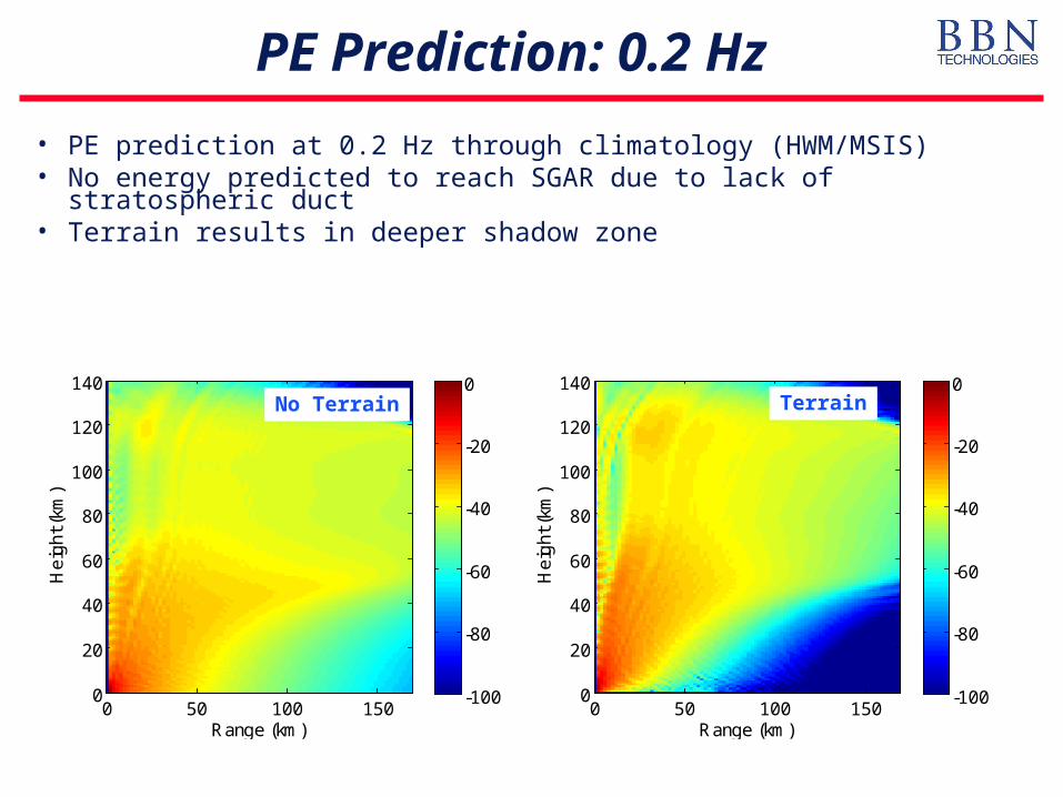
PE Prediction: 0.2 Hz

• PE prediction at 0.2 Hz through climatology (HWM/MSIS)• No energy predicted to reach SGAR due to lack of stratospheric duct• Terrain results in deeper shadow zone

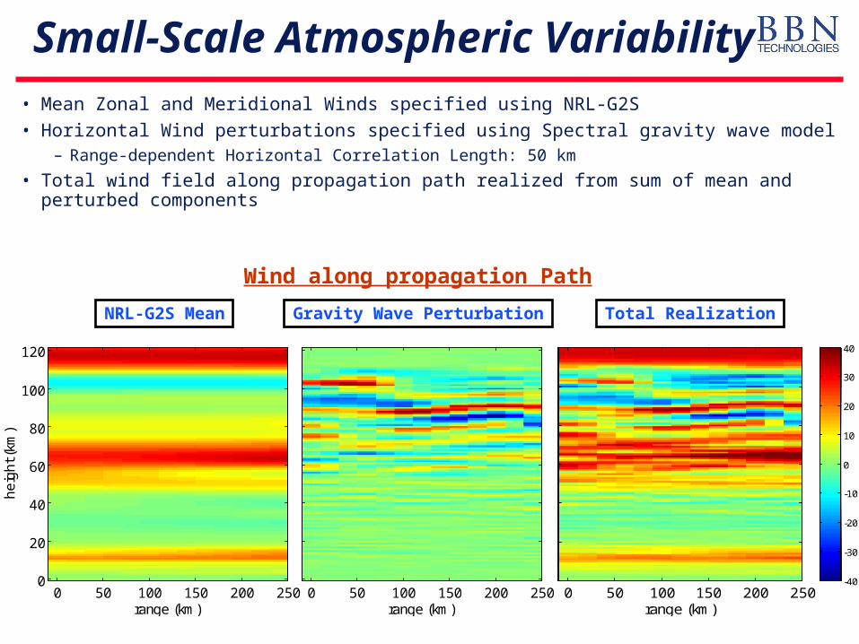
Small-Scale Atmospheric Variability• Mean Zonal and Meridional Winds specified using NRL-G2S

• Horizontal Wind perturbations specified using Spectral gravity wave model– Range-dependent Horizontal Correlation Length: 50 km

• Total wind field along propagation path realized from sum of mean and perturbed components

NRL-G2S Mean Total RealizationGravity Wave Perturbation

range (km)

he

igh

t (km

)

0 50 100 150 200 2500

20

40

60

80

100

120

-40

-30

-20

-10

0

10

20

30

40

range (km)

he

igh

t (km

)

0 50 100 150 200 2500

20

40

60

80

100

120

-40

-30

-20

-10

0

10

20

30

40

range (km)

He

igh

t (k

m)

0 50 100 150 200 2500

20

40

60

80

100

120

-40

-30

-20

-10

0

10

20

30

40

Wind along propagation Path

Range (km)

He

igh

t (km

)

PE with absorption: Amplitude Field (dB re 1 km)

0 50 100 1500

20

40

60

80

100

120

140

-100

-80

-60

-40

-20

0

Range (km)

He

igh

t (km

)

PE with absorption: Amplitude Field (dB re 1 km)

0 50 100 1500

20

40

60

80

100

120

140

-100

-80

-60

-40

-20

0

No Terrain Terrain

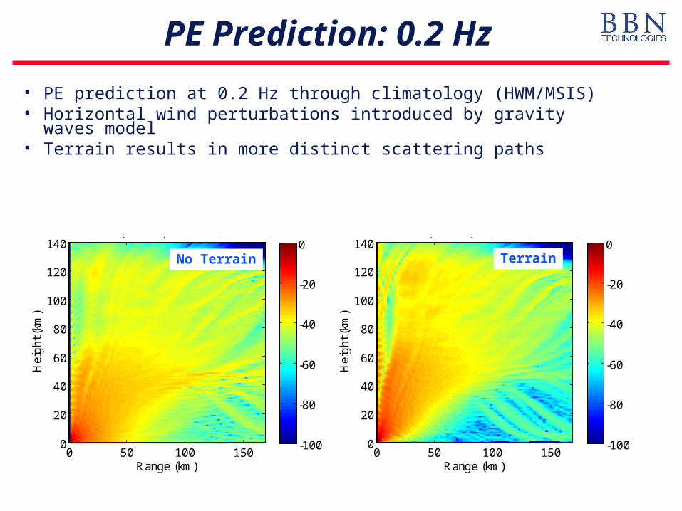
PE Prediction: 0.2 Hz

• PE prediction at 0.2 Hz through climatology (HWM/MSIS)• Horizontal wind perturbations introduced by gravity waves model• Terrain results in more distinct scattering paths

500 550 600 650 700-1

-0.5

0

0.5

1

Absolute Travel Time (sec)

Am

plit

ud

e (

Pa

)

500 550 600 650 700-1

-0.5

0

0.5

1

Absolute Travel Time (sec)

Am

plit

ud

e (

Pa

)

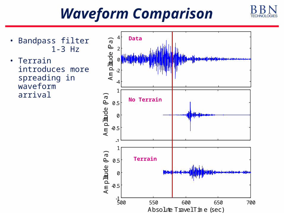
Waveform Comparison

• Bandpass filter 1-3 Hz

• Terrain introduces more spreading in waveform arrival -4

-2

0

2

4

Am

plit

ud

e (

Pa

)

No Terrain

Terrain

Data

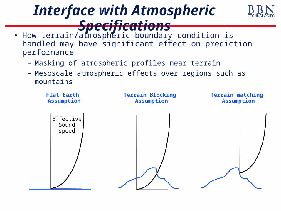
Interface with Atmospheric Specifications

• How terrain/atmospheric boundary condition is handled may have significant effect on prediction performance

– Masking of atmospheric profiles near terrain

– Mesoscale atmospheric effects over regions such as mountains

Terrain

Flat Earth Assumption

Terrain Blocking Assumption

EffectiveSoundspeed

Terrain matching Assumption

Conclusions and Future Research

• Preliminary Conclusions– Terrain appears to disperse down-range waveforms in cases where

significant terrain features are in proximity of source

• Issues for further research– Comparison of terrain masking, conformal mapping, and linear shift

mapping approaches – Sensitivity to ground impedance specification and its variability over

typical propagation paths– Required Topographic database resolution