Wave-scattering Formalisms for Multiport Energetic Systems

Pergamon 1. FrankIin Inst. Vol. 333(B). No. 4. 539-564. pp. 1996

sOOl6-0032(96)00019-l Copyright 0 1996 The Franklin Institute

Published by Elsevier Science Ltd Printed in Great Britain

0016-0032/96 SI5.00 + 0.00

Wave-scattering Formalisms for Multiport Energetic Systems

by RAUL G. LONGORIA

Department of Mechanical Engineering, University of Texas at Austin, Austin, TX 78712-1063, USA.

(Received 9 December 1995; accepted in revisedform 23 January 1996)

ABSTRACT: Thispaperpresentsa variant wave-scatteringapproachforphysicalsys- tern modeling and analysis that adopts duplexed wave signals to quantify thepropaga- tion, storage and dissipation of energy localized between and within system elements. This energetic perspective of wave-scattering techniques can exploit the relationship to bondgraph methods to complement techniques in multiport modeling and analysis. Examples arepresented that illustrate the use of wave-scattering methodsfor treating distributed-parameter eflects, nonlinear effects, and switching effects in system models. Furthermore, the methods presented lay the groundwork for extending network analysis and synthesis methods to multi-energy domain and mixed lumpedldistributed- parameter systems. Copyright @ 1996 Published by Elsevier Science Ltd

Z. Introduction

Energetic modeling of physical systems accounts for the flux, storage, and dissipation of energy, and employing such an approach has definite advantages in modeling a large class of systems. A case in point is the bond graph approach, which offers the added advantage of a well-formulated functional-graphical representation. The bond graph approach quantifies power flow between systems using a conjugate effort-flow pair, (e, f). An attractive feature of this method is the use of physical structure of a model to assign causality on bond connections between elements. Numerous extensions and applications of bond graph methods are found in the literature and in many textbooks. The success and popularity of this method for physical modeling arises from the fundamental yet highly adaptable basis of the approach. Paynter (1) has recounted how the bond graph method arose from a comprehensive study of many methods for system analysis. One method that played a contributing role in formulating bond graph fundamentals was the wave- scattering approach.

539

540 R. G. Longoria

This paper outlines the role that wave-scattering techniques can play in system modeling either alone or as a complementary method for analysis of subsystems. Recently, Paynter and Busch-Vishniac (2) reviewed fundamental physical and functional concepts underlying wave-scattering formalisms. Although implied, an explicit relationship to bond graph methods was not made in order to establish the scattering approach independently. Actually, Paynter had earlier discussed the role played by wave-scattering techniques on bond graph theory (3). Given the success of bond graph methods, however, one would be tempted to ask why and where a scattering formulation would be helpful. The formulation has, for the most part, remained confined to usage in circuit theory and physics. In these cases, the literature describing the use of scattering variables deals almost exclusively with linear systems. An exception is the extension for nonlinear systems suggested by Paynter and Busch-Vishniac, and further explored by Hogan (5).

The interest in scattering techniques continues to expand, as some of its most useful properties are exploited in different applications. Inspired by the work of Payn- ter and Busch-Vishniac, the relation between bond graphs and scattering methods was reported by Amara and Scavarda (6) and by Kamel and Dauphin-Tanguy (7). Following more closely the results from network theorists, Lilly and Anderson have also reported on the use of scattering variables in development of a modular approach for multi-robot control (8). The present paper endeavors to formulate a basis for continued work in wave-scattering approaches for generalized system modeling. An explicit connection to bond graphs is used to illustrate and in some cases clarify concepts under discussion. A goal of this paper is to present wave- scattering techniques that can be used to study linear or nonlinear, multi-energy representations of physical systems. Some examples are presented that illustrate when and how wave-scattering techniques can be useful.

II. Power Flow, Wave-scattering Variables, and Scattering Variables

The concept of power flux, taken from a continuum description, strictly refers to the product of a localized energy density and the rate by which this energy propagates. This concept is commonly used to account for the energy flux in media as governed by energy continuity principles, and is fundamental to an energetic modeling approach. In multiport system models, the exchange of energy between any two systems is accounted for by using macroscopic power flow quantities that, strictly speaking, are integrations of localized power flux across ports over a system surface. These fundamental notions underly the application of most power flow analysis procedures, including the bond graph method which quantifies a power flow using effort-flow (e, f ) conjugate variables.

A wave-scattering approach for modeling physical systems is also based on energy continuity, but a particular power flow mode is bisected into opposing components, a representation fundamental to wave motion descriptions. So while applicable to problems where energy is localized in a continuum, wave-scattering techniques employ a systems perspective that is attractive for studying lumped-parameter

Wave-scattering Formalisms 541

systems as well. In a wave-scattering representation, a single component of power flow, T, is composed of forepower, T, and backpower, T, flows such that, T = T - T . Each of these bilateral power flows represent the integration at a port of a scattering flux, which is defined as the product of a local scattering density and the local velocity of energy propagation. Employing this basis, we quantify the bilateral power flows using wave-scattering variables,

,~ = l ~ z and T = 1~2 , ~ w , (1)

where, ~ is a fore-directed wave-scattering variable, or forewave, and "~ is a back- directed wave-scattering variable, or backwave. These variables have units of root- power I, and can be graphically represented using a single power bond or by using duplex signal bonds; viz.,

W

The net power flow is considered positive in the fore-direction, and a factorization of the net power yields,

--*2 ,---2 T = ~ _ ~ w w 1 ~ 1

2 2 - ~ (w +"~) • - ~ (~ - "~) = e. f , (2)

which expresses the relationship between wave-scattering variables and the normalized (or scaled) effort, e, and flow, f , variables. Equation (2) relates homogeneous (in a unit basis sense) root-power conjugate variables (e, f ) to the wave-scattering variables (-ff,'~). This power factorization also reveals that the normalization by v~ commonly used in classical scattering representations (11-13) has a fundamentally physical basis. Note that the (e, f ) pair is related to non-normalized (un-scaled) effort and flow variables (e', f ' ) by a normalizing resistance (or impedance), e -- e ' / ~ , , and f = 4~'of ' , where the (e', f ' ) variables have physical units. The normalization by Ro will be discussed further in a later section.

To describe multiport system representations, scattering variables are defined at each port of the system or element. The scattering variables at a port are the inwave, u, and the outwave, v, and are distinguished from wave-scattering variables defined to quantify power flow between systems (e.g., on bonds). Scattering variables always adopt the convention that power is positive into a system such that Tin = u 2 / 2 - v2/2 . These definitions are illustrated in Fig. l(a) and (b), and illustrated further by the coupling of two systems in (b).

While the "sense" of each wave-scattering variable is imposed arbitrarily, the scattering variables at the port of a system are defined uniquely. Thus v is causally dependent on u and there is no need to make causal assignments in a scattering

I The square of the wave-scattering variable is adopted based on the relation between the scattering flux and the scattering density (9).

542 R. G. Longoria

u vl w u2

"S S " " " S l q • q 2 U 1 ~ ' - V2

(a) (b)

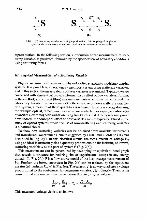
Fxc. 1. (a) Scattering variables at a single-port system. (b) Coupling of single-port systems via a wave-scattering bond and relation to scattering variables.

representation. In the following section, a discussion of the measurement of scattering variables is presented, followed by the specification of boundary conditions using scattering forms.

III. Physical Measurability o f a Scattering Variable

Physical measurement provides insight and is often essential to modeling complex systems. It is possible to characterize a multiport system using scattering variables, and in this section the measurability of these variables is examined. Typically, we are concerned with sensors that provide information on effort or flow variables. Further, voltage (effort) and current (flow) measures are basic to most instruments used in a laboratory. In order to characterize either the inwave or outwave scattering variables of a system, a measure of these quantities is required. In certain energy domains, for example optical, direct power measures are available. For example, radiometry quantifies electromagnetic radiation using transducers that directly measure power flow. Indeed, the concept of effort or flow variables are not typically defined in the study of optical systems, where the use of wave-scattering and scattering variables is a natural choice.

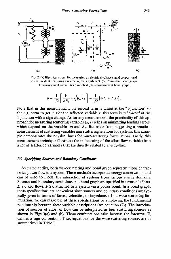
To show how scattering variables can be obtained from available instruments and transducers, we examine a circuit suggested by Carlin and Giordano (11) and illustrated in Fig. 2(a). In this electrical circuit, the measurement of voltage Vm using an ideal instrument yields a quantity proportional to the incident, or inwave, scattering variable u at the port of system S (Fig. 2(b)).

This measurement can be generalized by developing an equivalent bond graph that reveals a structure for realizing similar experimental setups in any energy domain. In Fig. 2(b), F is a flow source model of the ideal voltage measurement of Vm. Further, the boxed subsystem in Fig. 2(b) can be replaced by the equivalent gyrator (of modulus Ro/m) in Fig. 2(c). The current, I, is now gyrated into a voltage proportional to the root-power homogeneous variable, f ( t ) , directly. Then, using conventional measurement instrumentation this circuit sums voltages,

1 V R o i = v/2"Ro + V m - - - u .

m m m

This measured voltage yields u as follows,


I

, - ' o , i - 0 . . . . . V 0 l! ~/'= " , 0 I

I "as--':T I T:m ,n'/fou U ' -llll I " ° l R o l !

m

(a) (b) (e)

Fro. 2. (a) Electrical circuit for measuring an electrical voltage signal proportional to the incident scattering variable, u, for a system S. (b) Equivalent bond graph

of measurement circuit. (c) Simplified f ( t ) -measurement bond graph.

1 [~oRo ] 1 [e( t )+f( t )] U = ~ + ~ o ' I =~

Note that in this measurement, the second term is added at the "l-junction" to the e(t) term to get u. For the reflected variable v, this term is subtracted at the 1-junction with a sign change. As for any measurement, the practicality of this approach for measuring scattering variables (u, v) relies on minimizing loading errors, which depend on the variables m and Ro. But aside from suggesting a practical measurement of scattering variables and scattering relations for systems, this example demonstrates the physical basis for wave-scattering formulations. Lastly, this measurement technique illustrates the re-factoring of the effort-flow variables into a set of scattering variables that are directly related to energy-flux.

IV. Specifying Sources and Boundary Conditions

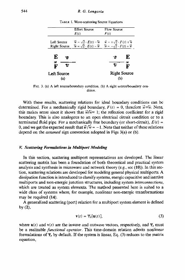
As stated earlier, both wave-scattering and bond graph representations characterize power flow in a system. These methods incorporate energy conservation and can be used to model the interaction of systems from various energy domains. Sources and boundary conditions in a bond graph are specified in terms of efforts, E(t), and flows, F(t), attached to a system via a power bond. In a bond graph, these specifications are convenient since sources and boundary conditions are typically given in terms of forces, velocities, or impedances. In a wave-scattering formulation, we can make use of these specifications by employing the fundamental relationship between these variable descriptions (see equation (2)). The introduction of sources of effort or flow can be interpreted as four scattering sources as shown in Figs 3(a) and (b). These combinations arise because the forewave, ~, defines a sign convention. Thus, equations for the wave-scattering sources are as summarized in Table I.

544 R. G. Longoria

TABLE I. Wave-scattering Source Equations

Effort Source Flow Source E(t) F(t)

Left Source ~ = ,/2. E(t) - ~ -ff = +-,~. F(t) +'~ Right Source ~ = x/2- E(t) --~ "~ = -v:2. F(t) +-ff

E E O f - - o r

F F Left Source Right Source

(a) (b)

FIG. 3. (a) A left source/boundary condition. (b) A right source/boundary condition.

With these results, scattering relations for ideal boundary conditions can be determined. For a mechanically rigid boundary, F ( t ) = 0, therefore ~--~. Note, this makes sense since it shows that ~ /~= 1; the reflection coefficient for a rigid boundary. This is also analogous to an open electrical circuit condition or to a terminated fluid pipe. For a mechanically free boundary (or short-circuit), E ( t ) =

0, and we get the expected result that ~ / ~ = - 1. Note that neither of these relations depend on the assumed sign convention adopted in Figs 3(a) or (b).

V. Scattering Formulations in Multiport Modeling

In this section, scattering multiport representations are developed. The linear scattering matrix has been a foundation of both theoretical and practical system analysis and synthesis in microwave and network theory (e.g., see (10)). In this section, scattering relations are developed for modeling general physical multiports. A dissipation function is introduced to classify systems, energic capacitive and inertive multiports and non-energic junction structures, including system interconnections,

which are treated as system elements. The method presented here is suited to a wide class of systems where, for example, nonlinear non-energic transformations may be required (14).

A generalized scattering (port) relation for a multiport system element is defined by (2),

v(t) = ~[u( t ) ] , (3)

where u(t) and v(t) are the inwave and outwave vectors, respectively, and Ys must be a realizable f u n c t i o n a l operator. This time-domain relation admits nonlinear formulations of ~'~ by default. If the system is linear, Eq. (3) reduces to the matrix equation,


v = S u, (4)

where S is the classical linear scattering matrix. For example, the one-port linear scattering relation is, v = S . u, which can be related to effort/flow variables by,

s _ V e - f z - 1 u - e +----f - z + 1 (5)

with z the normalized impedance z = e / f = Z/Ro = e' / ( f ' . Ro). A similar relation applies for n-port elements, and there exist relationships between the scattering matrix and the immittance matrices (impedance, Z, and admittance, Y), except for cases where the immittance matrices do not exist (e.g., ideal transformers).

5.1. A Dissipation Function from Thermodynamic Considerations

Consider a system described by the scattering relation of Eq. (3), rewritten in a multiplicative form suggested by Hogan (5),

~'s[u] = S(u) u. (6)

The difference between the incident and reflected power for a multiport system can be interpreted as entropy production, o-,

- - 1 r 1T 79-7 9 =~u u-~v v=T.f+=o', (7)

where T is absolute temperature and f~ is entropy flow rate (see also (17)). We define a dissipation function, D(u), in the relation,

1 T 1 + 1 T 1 T ~u u-~v v=~u [E-S(u)TS(u)]u=~u D(u)u. (8)

Here, D(u) = [ E - S(u)rS(u)], where E is the identity matrix. This dissipation function can now be used to define a conservative, or lossless, system as one in which o- = 0, which implies D(u) = 0 = [E - S(u)rS(u)], and that S(u) is orthogonal. The second law of thermodynamics will require that D(u) be positive semidefinite for any u. By introducing these concepts at this point in our discussion, we are able to (a) suggest the extended use of scattering techniques for thermodynamic systems modeling, and (b) present our basis for classifying systems and system elements.

5.2. Lossless scattering multiport elements

Scattering techniques have traditionally made use of representations for junctions and elements that can be pieced together to form system models (15,16). These building blocks are used in both analysis and synthesis, especially for systems where distinct elements having a specified constitutive behavior can be defined. The (normalized) scattering matrix has properties that restrict these defined elements and any system model to be physically realizable (2,12). As not all physical systems lend themselves to reticulation into elements and junctions, a more generally

546 R. G. Longoria

applicable scattering operator forms the basis for our development. In this section, we examine lossless scattering multiport element descriptions. For these systems, the dissipation function is zero (D = 0), which implies that either energy is being stored in lossless elements, or that it passes through conservatively. In either case, the scattering operator is orthogonal.

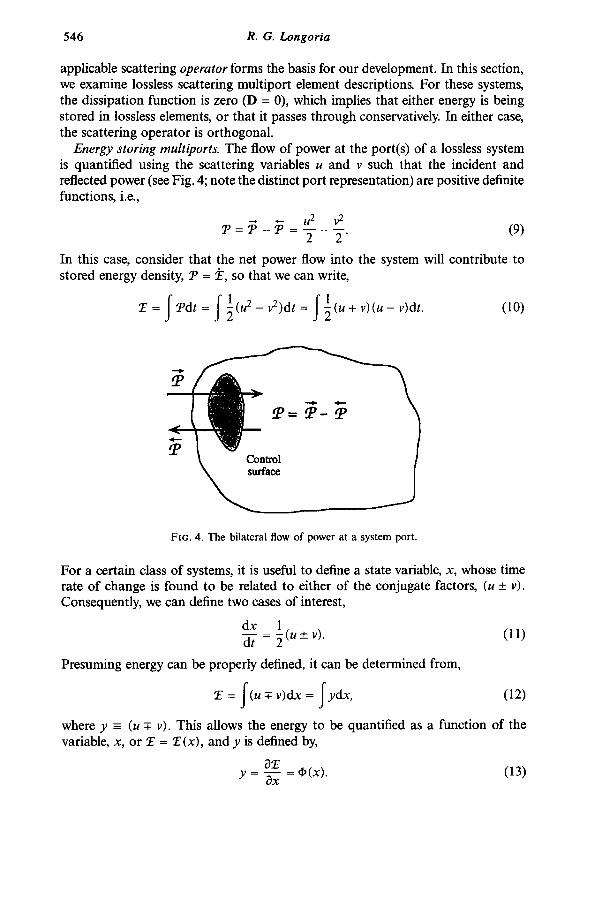
Energy storing multiports. The flow of power at the port(s) of a lossless system is quantified using the scattering variables u and v such that the incident and reflected power (see Fig. 4; note the distinct port representation) are positive definite functions, i.e.,

~ u 2 v 2 P = P - P = T - ~ (9)

In this case, consider that the net power flow into the system will contribute to stored energy density, P = 77, so that we can write,

E = f Pdt = ~ l (u2- v2)dt = ~ 1 ~(u + v)(u - v)dt. (10)

P

P

P = P - P

Control surface

FIG. 4. The b i la tera l flow of power at a sys tem port .

For a certain class of systems, it is useful to define a state variable, x, whose time rate of change is found to be related to either of the conjugate factors, (u _+ v). Consequently, we can define two cases of interest,

dx 1 d t = ~(u _+ v). (11)

Presuming energy can be properly defined, it can be determined from,

E = ~(u¥- v)dx= f ydx, (12)

where y - (u ¥ v). This allows the energy to be quantified as a function of the variable, x, or E = E(x), and y is defined by,

~E - ~ ( x ) . ( 1 3 ) Y - ~x

Wave-scattering F o r m a l i s m s 547

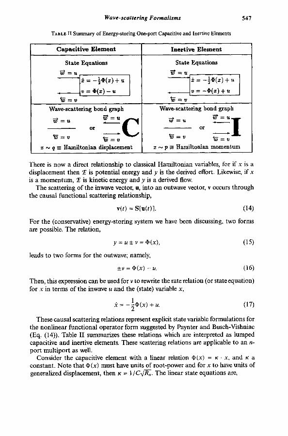
TABLE II Summary of Energy-storing One-port Capacitive and Inertive Elements

Capaci t ive E lement Inertive Element

State Equations

. = ~ ( x ) -

ti~ .= v

Wave-scattering bond graph

*X = v ~ = ~

x ~ q ~ Haaniltoniaa displacement

State Equations ]i)~ = u

. - ~ ( x ) + u ..J t i ~ = v

Wave-scattering bond graph

i i~= u or I ~ = v ~, = v

z N p _= Hamiltonian momentum

There is now a direct relationship to classical Hamiltonian variables, for if x is a displacement then T is potential energy and y is the derived effort. Likewise, if x is a momentum, T is kinetic energy and y is a derived flow.

The scattering of the inwave vector, u, into an outwave vector, v occurs through the causal functional scattering relationship,

v(t) = S[u(t)]. (14)

For the (conservative) energy-storing system we have been discussing, two forms are possible. The relation,

y = u + v = ~(x), (15)

leads to two forms for the outwave; namely,

_+v = ¢(x) - u. (16)

Then, this expression can be used for v to rewrite the rate relation (or state equation) for x in terms of the inwave u and the (state) variable x,

= - l ¢ ( x ) + u. (17)

These causal scattering relations represent explicit state variable formulations for the nonlinear functional operator form suggested by Paynter and Busch-Vishniac (Eq. (14)). Table I I summarizes these relations which are interpreted as lumped capacitive and inertive elements. These scattering relations are applicable to an n- port mult iport as well.

Consider the capacitive element with a linear relation ¢(x) = K • x, and K a constant. Note that ¢ (x) must have units of root-power and for x to have units of generalized displacement, then r = 1 / Cv~o. The linear state equations are,

548 R. G. Longoria

K y c = - ~ . x +u

I )= + K . X - - U

(18)

which gives x = u~ (s + r /2 ) so that,

K/2 - s - - u . (19) v - Kl2 + s

This linear scattering relation represents a linear lumped capacitive element. Fur- ther, if K = 2, then the generalized displacement q = 2x for a unit capacitance, C = 1. An identical result occurs for the inertive element with a generalized momentum p = 2x for a unit inertance, I = I. Note that the sign in Eq. (15) defining the variable y carries over into the linear scattering relations for the single-port C and I elements. These relations are identical except for sign; that is, for a unit lumped energy-storing element the linear scattering relation is given by,

1 - s ( 2 0 ) Se = *-1 + s ,

where the "+" refers to the capacitive element C and a " - " refers to the inertive element I. This binary nature of ideal energy-storing elements will be explored further in a section below on uniform transmission lines.

Non-Energic Multiports. Birkhoff (18) adopted the term non-energic to define a lossless dynamical system that stores no energy or for which stored energy is constant (i.e., 27 = 0). Representations of this type are ubiquitous in physical system modeling and are used to describe ideal interconnections or junction structure. A scheme proposed by Paynter (3, 19) is presented here to classify non-energic structures based on properties of their scattering representation. The classification scheme depends on the properties of the scattering matrix, S(u), which is orthogonal for a lossless system. Symmetric junction structures classified as Kron-Kirchhoff structures can include common effort and flow junctions and transformer elements. A general junction structure, which permits asymmetry in the scattering matrix, is classified as a Birkhoff-Tellegen structure, ascribed to Birkhoff who identified the need for a gyroscopic particle in the description of a non-energic (and Lagrangian) dynamical system (see (18), p. 24), and to Tellegen (20) for development of the gyrator as a network element and satisfying the need for a gyrator-like element in synthesis 2.

Table III summarizes the non-energic multiport concept and classification. De- tailed developments can be found in the literature. The Birkhoff-Tellegen structures are derived by considering any n-port representation and applying orthogonality. For the 2-port case, the condition of orthogonality on a non-energic multiport leads to transformer and gyrator representations. In the general case, these are inwave modulated device models. If constrained to be symmetric and with constant

2 As an aside, Tellegen recognized that Thomson and Tait and others had identified a need for gyroscopic terms in certain mechanics problems. However, it is Birkhoff and Tellegen's adaptations which have found more general application and are of direct relevance to modern multiport representations,

Wave-scattering Formalisms

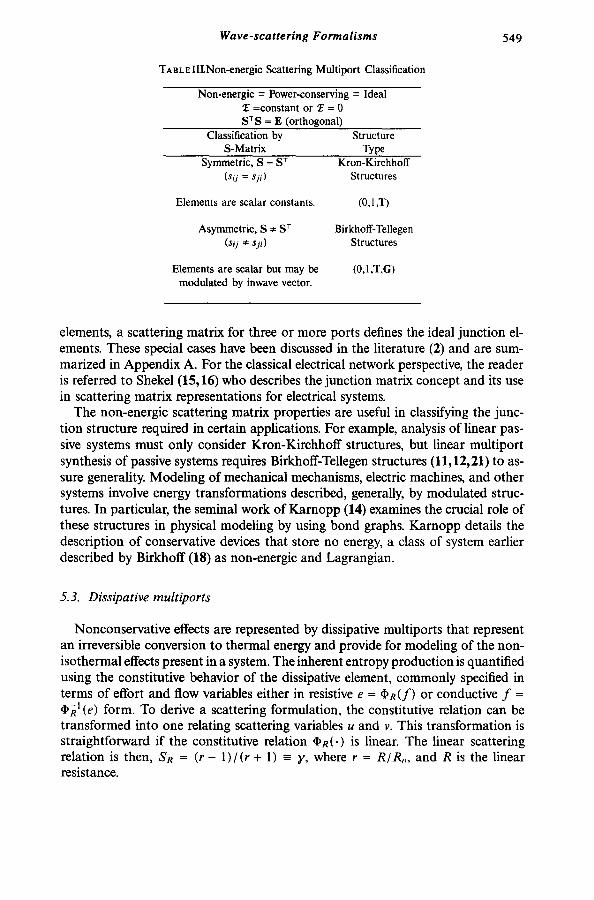
TABLEIII.Non-energic Scattering Multiport Classification

Non-energic = Power-conserving = Ideal 2? =constant or E = 0 SrS = E (orthogonal)

Classification by Structure S-Matrix Type

Symmetric, S = S r Kron-Kirchhoff ( s i j = s j i ) Structures

Elements are scalar constants. (0,1,T)

Asymmetric, S * S r Birkhoff-Tellegen (sij ~ sji) Structures

Elements are scalar but may be modulated by inwave vector.

(0,1 ,T,G)

549

elements, a scattering matrix for three or more ports defines the ideal junction elements. These special cases have been discussed in the literature (2) and are summarized in Appendix A. For the classical electrical network perspective, the reader is referred to Shekel (15,16) who describes the junction matrix concept and its use in scattering matrix representations for electrical systems.

The non-energic scattering matrix properties are useful in classifying the junction structure required in certain applications. For example, analysis of linear passive systems must only consider Kron-Kirchhoff structures, but linear multiport synthesis of passive systems requires Birkhoff-Tellegen structures (11,12,21) to as- sure generality. Modeling of mechanical mechanisms, electric machines, and other systems involve energy transformations described, generally, by modulated structures. In particular, the seminal work of Karnopp (14) examines the crucial role of these structures in physical modeling by using bond graphs. Karnopp details the description of conservative devices that store no energy, a class of system earlier described by Birkhoff (18) as non-energic and Lagrangian.

5.3. Dissipative multiports

Nonconservative effects are represented by dissipative multiports that represent an irreversible conversion to thermal energy and provide for modeling of the non- isothermal effects present in a system. The inherent entropy production is quantified using the constitutive behavior of the dissipative element, commonly specified in terms of effort and flow variables either in resistive e = ~R(f ) or conductive f = • R 1 (e) form. To derive a scattering formulation, the constitutive relation can be transformed into one relating scattering variables u and v. This transformation is straightforward if the constitutive relation ~R(') is linear. The linear scattering relation is then, SR = ( r - 1) / ( r + 1) = y, where r = R/R,, , and R is the linear resistance.

550 R. G. Longoria

m ot

, 1T ,2 R R f l A vl v2

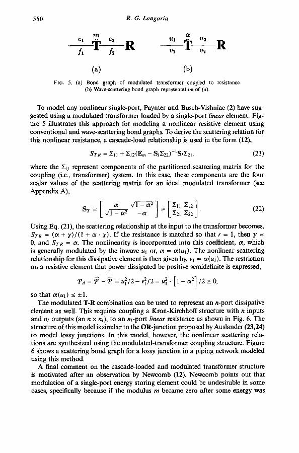
FIG. 5. (a)

(a) (b) Bond graph of modulated transformer coupled to resistance. (b) Wave-scattering bond graph representation of (a).

To model any nonlinear single-port, Paynter and Busch-Vishniac (2) have suggested using a modulated transformer loaded by a single-port linear element. Fig- ure 5 illustrates this approach for modeling a nonlinear resistive element using conventional and wave-scattering bond graphs. To derive the scattering relation for this nonlinear resistance, a cascade-load relationship is used in the form (12),

STR ---- ~11 + ~ 1 2 ( E m - S / ~ 2 2 ) - l S l ~ 2 1 , (21)

where the Eq represent components of the partitioned_ scattering matrix for the coupling (i.e., transformer) system. In this case, these components are the four scalar values of the scattering matrix for an ideal modulated transformer (see Appendix A),

S T = = ~21 E22 "

Using Eq. (21), the scattering relationship at the input to the transformer becomes, SrR = (a + y)/(1 + tx • y). I f the resistance is matched so that r = l, then y = 0, and S r R = ¢¢. The nonlinearity is incorporated into this coefficient, a, which is generally modulated by the inwave ul or, a -- o~(ul). The nonlinear scattering relationship for this dissipative element is then given by, Vl = or(u1). The restriction on a resistive element that power dissipated be positive semidefinite is expressed,

Pd = P - p = u 2 / 2 - v2/E = u 2 " [ 1 - ° ¢ 2]/2>__ 0,

so that a(Ul) _< _1. The modulated T-R combination can be used to represent an n-port dissipative

element as well. This requires coupling a Kron-Kirchhoff structure with n inputs and nt outputs (an n x nt), to an nt-port linear resistance as shown in Fig. 6. The structure of this model is similar to the OR-junction proposed by Auslander (23,24) to model lossy junctions. In this model, however, the nonlinear scattering relations are synthesized using the modulated-transformer coupling structure. Figure 6 shows a scattering bond graph for a lossy junction in a piping network modeled using this method.

A final comment on the cascade-loaded and modulated transformer structure is motivated after an observation by Newcomb (12). Newcomb points out that modulation of a single-port energy storing element could be undesirable in some cases, specifically because if the modulus m became zero after some energy was


l r

/ 1

1

.a.l I i T - - ~ I Rs

I I

I I

I I II

l~o,,..euemc ( K n ~ - ~ Su.uctm Dissil~ve Held

0

1

"lossy fluid junction"

(a) (b) FIG. 6. (a) Multiport representation for a (b) nonlinear dissipative fluid junction.

stored and remained so thereafter, then the functionality of this element could be compromised; i.e., it would seem to model a dissipative rather than a lossless process. It is not too difficult, however, to envision where such a situation might actually be needed, such as in modeling decoupling of systems through a clutch (or switch) or for analyzing the effect of "wave traps" that absorb incoming waves. In this way, modulated coupling elements are fundamental for representing power dissipation.

5.4. The uniform uni-power transmission line

The wave-scattering approach was earlier related in this paper to concepts of energy-flux and wave-power propagation at a field continuum level. However, the emphasis up to this point has been on lumped-parameter multiport representations. An alternative introduction to scattering representations can be derived by considering the field or continuum basis, and such an approach is the topic of a related paper (9). We can, however, incorporate distributed-parameter effects in our system models by introducing in the present discussion a uniform "line" element, or "U- line" (25). A U-line represents a passive transmitter of (single or uni-) power with uniformly distributed properties. A one-dimensional lossless U-line storing both kinetic and potential energy is a wavelike transmitter governed by the wave equation and will be referred to as a W-line. Similarly, a one-dimensional lossy U-line for representing diffusive power propagation can be referred to as an H-line. The description of these line models can be developed directly from lumped-parameter representations as shown by Paynter (22) and Beaman and Paynter (25). As an example, consider a two-port wave-scattering bond graph element for a W-line as,

W

5 5 2 R. G. Longoria

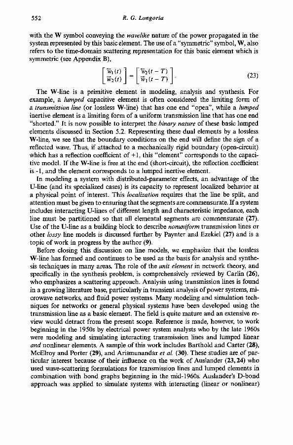
with the W symbol conveying the wavelike nature of the power propagated in the system represented by this basic element. The use of a "symmetric" symbol, W, also refers to the time-domain scattering representation for this basic element which is symmetric (see Appendix B),

W 2 ( t ) = L W l ( t - T ) "

The W-line is a primitive element in modeling, analysis and synthesis. For example, a lumped capacitive element is often considered the limiting form of a transmission line (or lossless W-line) that has one end "open", while a lumped inertive element is a limiting form of a uniform transmission line that has one end "shorted." It is now possible to interpret the binary nature of these basic lumped elements discussed in Section 5.2. Representing these dual elements by a lossless W-line, we see that the boundary conditions on the end will define the sign of a reflected wave. Thus, if attached to a mechanically rigid boundary (open-circuit) which has a reflection coefficient of + 1, this "element" corresponds to the capacitive model. If the W-line is free at the end (short-circuit), the reflection coefficient is -1, and the element corresponds to a lumped inertive element.

In modeling a system with distributed-parameter effects, an advantage of the U-line (and its specialized cases) is its capacity to represent localized behavior at a physical point of interest. This localization requires that the line be split, and attention must be given to ensuring that the segments are commensurate. Ifa system includes interacting U-lines of different length and characteristic impedance, each line must be partitioned so that all elemental segments are commensurate (27). Use of the U-line as a building block to describe nonuniform transmission lines or other lossy line models is discussed further by Paynter and Ezekiel (27) and is a topic of work in progress by the author (9).

Before closing this discussion on line models, we emphasize that the lossless W-line has formed and continues to be used as the basis for analysis and synthesis techniques in many areas. The role of the unit element in network theory, and specifically in the synthesis problem, is comprehensively reviewed by Carlin (26), who emphasizes a scattering approach. Analysis using transmission lines is found in a growing literature base, particularly in transient analysis of power systems, microwave networks, and fluid power systems. Many modeling and simulation techniques for networks or general physical systems have been developed using the transmission line as a basic element. The field is quite mature and an extensive re- view would detract from the present scope. Reference is made, however, to work beginning in the 1950s by electrical power system analysts who by the late 1960s were modeling and simulating interacting transmission lines and lumped linear and nonlinear elements. A sample of this work includes Barthold and Carter (28), McElroy and Porter (29), and Arismunandar et al. (30). These studies are of particular interest because of their influence on the work of Auslander (23, 24) who used wave-scattering formulations for transmission lines and lumped elements in combination with bond graphs beginning in the mid-1960s. Auslander's D-bond approach was applied to simulate systems with interacting (linear or nonlinear)


lumped elements and transmission lines, and inspired follow-on studies by Tsai and others (31-33). As an aside, the TLM (transmission-line modeling) method, cred- ited to Johns (34), has similar attributes and has been advanced in the literature in recent years.

VI. Examples o f Wave-scattering Usage

This section presents some example uses of a wave-scattering approach, focusing on certain aspects of each problem that motivate or benefit from this methodology. The intent is to illustrate how scattering techniques can be applied in a wide class of physical problems, including systems with nonlinearity.

6.1. Interacting lumped and distributed parameter systems

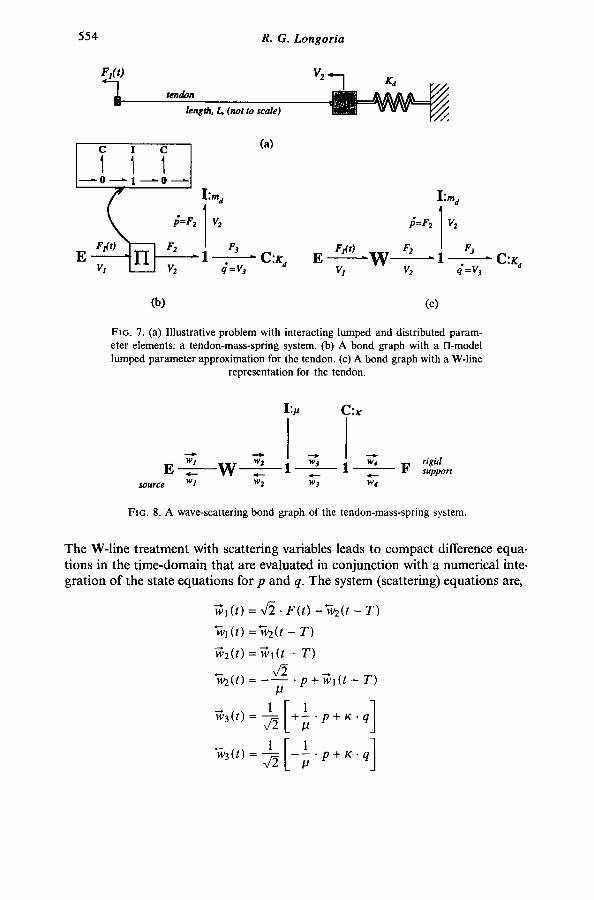
There exist many practical and theoretical obstacles in developing models of systems composed of components classified as lumped interacting with components having distributed parameter effects. Difficulties arise particularly when nonlinear- ities exist in the lumped elements, such as in hydraulic systems where fluid lines interact with nonlinear system elements (valves, motors, etc.). In the example that follows, the intent was to illustrate the merging of scattering techniques with the state space methods which are prevalent in modern system analysis. A relatively simple system was selected to demonstrate these concepts and is illustrated in Fig. 7(a). This system consists of a tendon or cable, a one-dimensional transmission line, interacting with components best described as lumped elements. Although these lumped elements were treated with linear constitutive relations in this example, including nonlinear effects would offer no difficulty to the present analysis.

The analysis of this system was conducted in two ways, one by making a lumped approximation and another using an exact (time-domain) scattering representation to account for the distributed nature of the tendon. These two approaches are illustrated by the bond graphs of Figs 7(b) and (c). The tendon is represented by a lumped H-model in (b) and by a lossless W-line in (c). Analysis using the 1-l- model proceeds in a conventional manner (with effort-flow variables). To analyze the system with the W-line, we develop the wave-scattering bond graph illustrated in Fig. 8. The parameters on the lumped elements are defined as, p = m d / ~ and r = /~t/.v/-~,., where Zc is the characteristic impedance of the tendon. Also, note that the power flow on bond 4 is zero and has no effect for the present analysis. The scattering equations for this system are coupled to state equations for the mass momentum, p, and the spring displacement, q. From the bond graph, these state equations can be derived in terms of wave-scattering variables as,

1 -

1 - % ) ]

554 R. G. Longor ia

F,(0

tendon

length, L, (not to scale)

v~

v, *~_.1__l

I:%

F2 1

I/2

(a)

I'ra d

:=e2 ] v2 ej .C:Ka E F ~ ( 0 . W F, . ,%

4=v, v, v~ 4=v,

Co) (c)

FIG. 7. (a) Illustrative problem with interacting lumped and distributed parameter elements: a tendon-mass-spring system. (b) A bond graph with a H-model lumped parameter approximation for the tendon. (c) A bond graph with a W-line

representation for the tendon.

I

E w ~ . _ . ~ W _ _ _ ~ 1 ~,~ . ic .--

$ourc~ wl W2 W3

C:~

-'~ rigid 1 W4 F support

W4

FIG. 8. A wave-scattering bond graph of the tendon-mass-spring system.

- C:K~

The W-line treatment with scattering variables leads to compact difference equations in the time-domain that are evaluated in conjunction with a numerical integration of the state equations for p and q. The system (scattering) equations are,

-if1 ( t) = x/2 . F ( t ) -'w2(t - T)

"WI (t) ='WE(t -- T )

~2(t) = ~ j ( t - T) 4~

~2(t) . . . . p + ~ l ( t - T) /J

~ 3 ( t ) = " ~ + ~ - p + r . q

~3(t) = ~ - - ~ . ? + K . q


where F(t) = El (t)/v~cc, is the normalized force. A step force was applied at the end of the tendon as indicated in Fig. 7(a). For this forcing, and with the tendon unstretched at t = 0, the displacement time-histories of the lumped mass (or spring) as predicted by the two models are contrasted in Fig. 9. For this problem, it is evident that the 11 model approximation deviates from the result found using the W-line model, which more accurately represents the tendon dynamics. The decision to ignore distributed effects in a system often relies on whether the lowest wavelength of a disturbance is larger than a characteristic length of the system (e.g., L). This rule works well when the wave transmission occurs in an isolated element or under periodic forcing. When the distributed element is part of a larger system the usefulness of this criterion is not certain.

x 10 "6 12

Lumped Mass/Spring Displacement, m

10

8

6

| ' ~J

J~ 2

c~ 0

-2

-4

-6 0 10 20 30 40

Dimensionless Time, t/l" 50

FIG. 9. A comparison of results from a scattering simulation with a W-line model of a tendon versus results for a l-l-model for the tendon.

6.2. Examples of scattering interfaces

In this section, we examine the use of wave-scattering formulations to model physical interfaces that transmit, reflect, and/or absorb power. These physical elements are classified here as scattering interfaces, and this classification includes, as examples, frictional couplings (e.g., clutching systems) and electrical switches. Clearly not an exhaustive set, these examples exemplify elements of a system that

556 R. G. Longoria

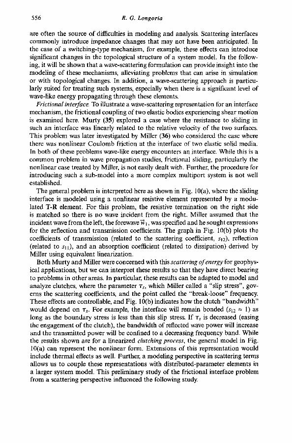
are often the source of difficulties in modeling and analysis. Scattering interfaces commonly introduce impedance changes that may not have been anticipated. In the case of a switching-type mechanism, for example, these effects can introduce significant changes in the topological structure of a system model. In the following, it will be shown that a wave-scattering formulation can provide insight into the modeling of these mechanisms, alleviating problems that can arise in simulation or with topological changes. In addition, a wave-scattering approach is particularly suited for treating such systems, especially when there is a significant level of wave-like energy propagating through these elements.

Frictional interface. To illustrate a wave-scattering representation for an interface mechanism, the frictional coupling of two elastic bodies experiencing shear motion is examined here. Murty (35) explored a case where the resistance to sliding in such an interface was linearly related to the relative velocity of the two surfaces. This problem was later investigated by Miller (36) who considered the case where there was nonlinear Coulomb friction at the interface of two elastic solid media. In both of these problems wave-like energy encounters an interface. While this is a common problem in wave propagation studies, frictional sliding, particularly the nonlinear case treated by Miller, is not easily dealt with. Further, the procedure for introducing such a sub-model into a more complex multiport system is not well established.

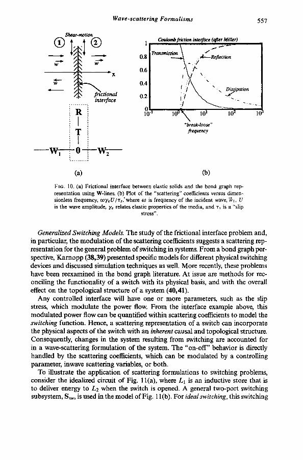
The general problem is interpreted here as shown in Fig. 10(a), where the sliding interface is modeled using a nonlinear resistive element represented by a modulated T-R element. For this problem, the resistive termination on the right side is matched so there is no wave incident from the right. Miller assumed that the incident wave from the left, the forewave ~ j, was specified and he sought expressions for the reflection and transmission coefficients. The graph in Fig. 10(b) plots the coefficients of transmission (related to the scattering coefficient, sl2), reflection (related to sl 1), and an absorption coefficient (related to dissipation) derived by Miller using equivalent linearization.

Both Murty and Miller were concerned with this scattering of energy for geophysical applications, but we can interpret these results so that they have direct bearing to problems in other areas. In particular, these results can be adapted to model and analyze clutches, where the parameter r,, which Miller called a "slip stress", gov- erns the scattering coefficients, and the point called the "break-loose" frequency. These effects are controllable, and Fig. 10(b) indicates how the clutch "bandwidth" would depend on 7s. For example, the interface will remain bonded (sl2 = I) as long as the boundary stress is less than this slip stress. If "r., is decreased (easing the engagement of the clutch), the bandwidth of reflected wave power will increase and the transmitted power will be confined to a decreasing frequency band. While the results shown are for a linearized clutching process, the general model in Fig. 10(a) can represent the nonlinear form. Extensions of this representation would include thermal effects as well. Further, a modeling perspective in scattering terms allows us to couple these representations with distributed-parameter elements in a larger system model. This preliminary study of the frictional interface problem from a scattering perspective influenced the following study.

W a v e - s c a t t e r i n g F o r m a l i s m s 557

Shear.motion

W

tctional efface

R I

T I

wr2-.; o

1

0.8

0.6

0.4

0.2

Coulomb frictlon interface (after #liller )

" breok.loose " frequency

(a) (b)

FIo. 10. (a) Frictional interface between elastic solids and the bond graph representation using W-lines. (b) Plot of the "scattering" coefficients versus dimensionless frequency, ooy~Ul'r.,,'where to is frequency of the incident wave, ~ t , U is the wave amplitude, Ye relates elastic properties of the media, and "rs is a "slip

stress".

Generalized Switching Models. The study of the frictional interface problem and, in particular, the modulation of the scattering coefficients suggests a scattering representation for the general problem of switching in systems. From a bond graph perspective, Karnopp (38,39) presented specific models for different physical switching devices and discussed simulation techniques as well. More recently, these problems have been reexamined in the bond graph literature. At issue are methods for rec- onciling the functionality of a switch with its physical basis, and with the overall effect on the topological structure of a system (40,41).

Any controlled interface will have one or more parameters, such as the slip stress, which modulate the power flow. From the interface example above, this modulated power flow can be quantified within scattering coefficients to model the switching function. Hence, a scattering representation of a switch can incorporate the physical aspects of the switch with an inherent causal and topological structure. Consequently, changes in the system resulting from switching are accounted for in a wave-scattering formulation of the system. The "on-off" behavior is directly handled by the scattering coefficients, which can be modulated by a controlling parameter, inwave scattering variables, or both.

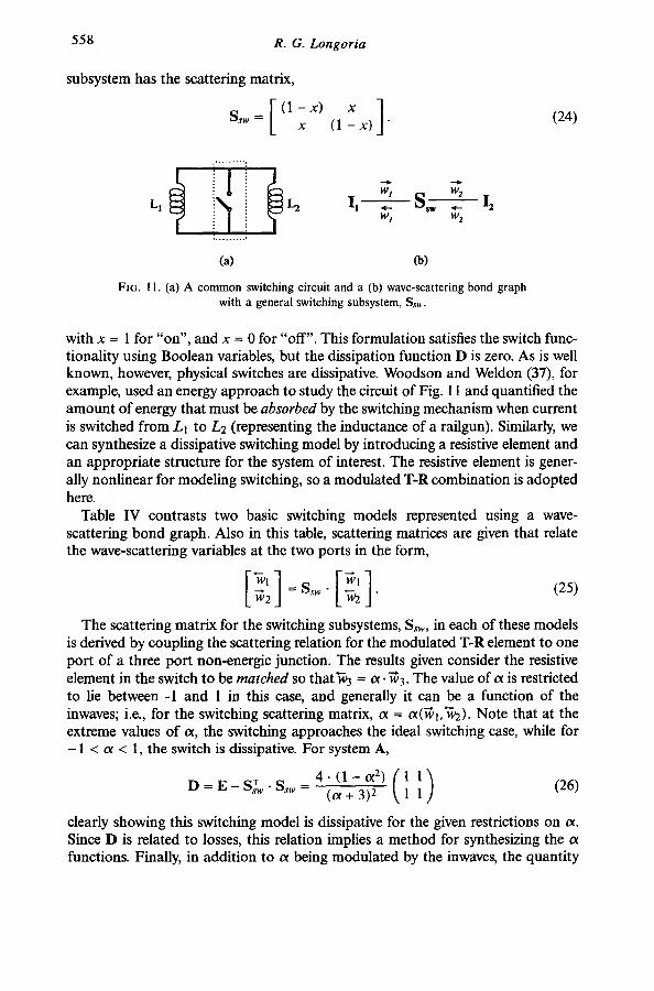
To illustrate the application of scattering formulations to switching problems, consider the idealized circuit of Fig. ll(a), where LI is an inductive store that is to deliver energy to L2 when the switch is opened. A general two-port switching subsystem, S.~w, is used in the model of Fig. 11 (b). For ideal switching, this switching

558 R. G. Longoria

subsystem has the scattering matrix,

Ssw= [ (1-x) x ] x (1 - x ) "

(24)

I

w~ w 2 LI L2 It ~ S.w ~ 12

W 1 W 2

. . . . . . . . . .

(a) (b)

FIG. 11. (a) A common switching circuit and a (b) wave-scattering bond graph with a general switching subsystem, Ss~:.

with x = 1 for "on", and x = 0 for "off". This formulation satisfies the switch functionality using Boolean variables, but the dissipation function D is zero. As is well known, however, physical switches are dissipative. Woodson and Weldon (37), for example, used an energy approach to study the circuit of Fig. 11 and quantified the amount of energy that must be absorbed by the switching mechanism when current is switched from Ll to L2 (representing the inductance of a railgun). Similarly, we can synthesize a dissipative switching model by introducing a resistive element and an appropriate structure for the system of interest. The resistive element is generally nonlinear for modeling switching, so a modulated T-R combination is adopted here.

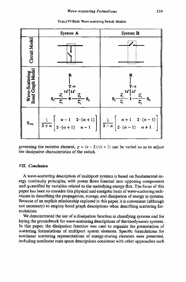
Table IV contrasts two basic switching models represented using a wave- scattering bond graph. Also in this table, scattering matrices are given that relate the wave-scattering variables at the two ports in the form,

The scattering matrix for the switching subsystems, Ssw, in each of these models is derived by coupling the scattering relation for the modulated T-R element to one port of a three port non-energic junction. The results given consider the resistive element in the switch to be matched so t h a t ~ = a . N3. The value of o~ is restricted to lie between -1 and 1 in this case, and generally it can be a function of the inwaves; i.e., for the switching scattering matrix, o~ --- o~(N1,%2). Note that at the extreme values of o~, the switching approaches the ideal switching case, while for - 1 < oc < 1, the switch is dissipative. For system A,

D = E _ S r .S~w. _ 4 - ( 1 - c t 2)(_~+3~ (11 11) (26)

clearly showing this switching model is dissipative for the given restrictions on o~. Since D is related to losses, this relation implies a method for synthesizing the ot functions. Finally, in addition to ot being modulated by the inwaves, the quantity

Wave-scattering Formalisms

TABLE IV. Basic Wave-sca t te r ing Switch Mode l s

559

"5 .2

!

m

$8~o

S,

System A System B

t

• i

R

I T : a

w t w~ ~_ 0 - - ' -~- - S, wl w 2

1 a - 1 2 . ( a + 1 )

3 + a 2 - ( a - k l ) a - 1 .[

i / . !

J

R

I T:a

% w2

i 1 a + 1 2 . ( a - 1)

3 - a 2 . ( ~ - 1) ~ + 1

governing the resistive element, y = ( r - 1)/(r + 1) can be varied so as to adjust the dissipative characteristics of the switch.

VII. Conclusion

A wave-scattering description of multiport systems is based on fundamental energy continuity principles, with power flows bisected into opposing components and quantified by variables related to the underlying energy-flux. The focus of this paper has been to consider this physical and energetic basis of wave-scattering techniques in describing the propagation, storage, and dissipation of energy in systems. Because of an explicit relationship explored in this paper, it is convenient (although not necessary) to employ bond graph descriptions when describing scattering formulations.

We demonstrated the use of a dissipation function in classifying systems and for laying the groundwork for wave-scattering descriptions of thermodynamic systems. In this paper, the dissipation function was used to organize the presentation of scattering formulations of multiport system elements. Specific formulations for nonlinear scattering representations of energy-storing elements were presented, including nonlinear state space descriptions consistent with other approaches such

560 R. G. Longoria

as the bond graph method. In addition, non-energic and dissipative scattering multiport models were examined.

An example was presented to demonstrate how wave-scattering methods can be used to model and analyze systems with interacting lumped and distributed elements. A companion paper under preparation by this author extends the use of the line elements presented here to show how wave-scattering representations are useful in modeling more complex distributed-parameter systems.

We introduced the concept of a scattering interface for analyzing practical physical problems such as frictional coupling. The approach was used to suggest a scattering approach for generalized switching problems. The idea of using a scattering approach is particularly useful when dealing with switching because changes in the functional as well as causal and topological aspects of a system can be incorporated. Some fundamental results in this area were presented, suggesting continued development of scattering representations for modeling switching and switching systems.

Acknowledgments

The author gratefully acknowledges the support, encouragement, and intellectual tutelage of Professor Henry M. Paynter.

This paper describes results from research supported by the National Science Foundation through grant number CMS-9410654, under the direction of Dr Devendra E Garg.

References

(1) H.M. Paynter, "An Epistemic Prehistory of Bond Graphs", Bond Graphs for Engineers, ed. P.C. Breedveld and G. Dauphin-Tanguy, Elsevier Science, North-Holland, 1992.

(2) H.M. Paynter and I. Busch-Vishniac, "Wave-scattering Approaches to Conservation and Causality", Journal of the Franklin Institute, Vol. 325, No. 3, pp. 295-313, 1988.

(3) H.M. Paynter, Discussion of." "The Properties of Bond Graph Junction Structure Ma- trices", Journal of Dynamic Systems, Measurement and Control, Vol. 98, pp. 209-210, 1976.

(4) ET. Brown, "A Unified Approach to the Analysis of Uniform One-Dimensional Dis- tributed Systems", Journal of Basic Engineering, Vol. 89, No. 2, pp. 423-432, 1967.

(5) N. Hogan, "Geometrical analysis of isenergic junction structures", Bond Graphs for Engineers, Ed. P.C. Breedveld and G. Dauphin-Tanguy, Elsevier Science, North- Holland, pp. 57-65, 1992.

(6) M. Amara and S. Scavarda, "A Procedure to Match Bond Graph and Scattering Formalisms", Journal of the Franklin Institute Vol. 328, No. 5/6, pp. 887-899, 1991.

(7) A. Kamel and G. Dauphin-Tanguy. 1993, "Bond Graph Modeling of Power Waves in the Scattering Formalism", lnt. Conference on Bond Graph Modeling and Simulation (ICBGM'93), San Diego, California, pp. 41-46.

(8) K.W. Lilly and R.J. Anderson, "A Modular Approach to Multi-Robot Control," submitted to IEEE Transactions on Robotics and Automation, August 1995.


(9) R.G. Longoria, "Duplexed Energy-Flux and Wave-Power in Wave-Scattering For- malisms", To be submitted to Journal of the Franklin Institute, March 1996.

(10) C.G. Montgomery, R.H. Dicke, and E.M. Purcell, "Principles of Microwave Circuits", McGraw-Hill, New York, 1948. (Reprinted by Dover, 1965.)

(11) H.J. Carlin and A.B. Giordano, "Network Theory: An Introduction to Reciprocal and Nonreciprocal Circuits", Prentice-Hall, Englewood Cliffs, N.J., 1964.

(12) R.W Newcomb, "Linear Multiport Synthesis", McGraw-Hill, New York, 1966. (13) V. Belevitch, "Classical Network Theory", Holden-Day, San Francisco, 1968. (14) D. Karnopp, "Power-conserving Transformations: Physical Interpretations and Appli-

cations using Bond Graphs", Journal of the Franklin Institute, Vol. 288, No. 3, pp. 175-201, 1969.

(15) J. Shekel, "On the Analysis of Scattering Networks", Proceedings of lOth Annual Allerton Conference, pp. 700-708, 1972.

(16) J. Shekel, "The Junction Matrix in the Analysis of Scattering Networks", IEEE Trans- actions on Circuits and Systems, Vol. CAS-21, No. 1, pp. 21-25, 1974.

(17) S.R. de Groot and P. Mazur, "Non-Equilibrium Thermodynamics", North-Holland Publishing Company, Amsterdam, 1962. Unabridged, corrected Dover edition, 1984.

(18) G.D, Birkhoff, "Dynamical Systems", American Mathematical Society, Providence, 1927.

(19) H.M. Paynter, Discussion of." "State-Space Formulation for Bond Graphs of Multiport Systems", by R.C. Rosenberg, Journal of Dynamic Systems, Measurement and Control, Vol. 93, pp. 123-124, 1971.

(20) B.D.H. Tellegen, "The Gyrator, A New Electric Network Element", Philips Research Reports, Vol. 3, pp. 81-101, 1948.

(21) R.W. Newcomb, "Active Integrated Circuit Synthesis", Prentice-Hall, Englewood Cliffs, N.J., 1968.

(22) H.M. Paynter, "Analysis and Design of Engineering Systems", MIT Press, Cambridge, Massachusetts, 1961.

(23) D.M. Auslander, "Analysis of Networks of Wavelike Transmission Elements", ScD Thesis, Engineering Projects Laboratory, M.I.T., August 1966.

(24) D.M. Auslander, "Distributed System Simulation With Bilateral Delay-Line Models", Journal of Basic Engineering, Vol. 90, No. 2, pp. 195-200, 1968.

(25) J.J. Beaman and H.M. Paynter, Modeling of Physical Systems, Book in progress and to be published by Harper and Row. Chapter 8.

(26) H.J. Carlin, "Distributed Circuit Design with Transmission Line Elements", Proc of the IEEE Circuit Theory, Vol. 59, No. 7, pp. 1059-1081, 1971.

(27) H.M. Paynter and ED. Ezekiel, "Water Hammer in Nonuniform Pipes as an Example of Wave Propagation in Gradually Varying Media", Trans. ASME, Vol. 58, pp. 1585- 1595, 1959.

(28) L.O, Barthold and G.K. Carter, "Digital Traveling-Wave Solutions", Trans. of AIEE, Vol. 80, Pt. 3, pp. 812-820, 1961.

(29) A.J. McElroy and R.M. Porter, "Digital Computer Calculation of Transients in Electric Networks", Trans. ofAIEE, Vol. 82, Pt. 3, pp. 88-96, 1963.

(30) A. Arismunandar, W.S. Price and A.J. McElroy, "A Digital Computer Iterative Method for Simulating Switching Surge Responses of Power Transmission Networks", Trans. ofAIEE, Vol. 83, Pt. 3, pp. 356-368, 1964.

(31) N.T. Tsai, "Analysis of Nonlinear Transient Motion of Cables Using Bond Graph Method", Journal of Engineering for Industry, Vol. 94, pp. 500-506, 1972.

(32) N.T. Tsai and S.M. Wang, "Delay-Bond Graph Models for Geared Torsional Systems", Journal of Applied Mechanics, pp. 366-370 (Paper No. 73-APMW-33), 1974.

562 R. G. Longoria

(33) D. M. Auslander, N.T. Tsai and E Farazian. 1975, "Bond Graph Models for Torsional Energy Transmission", Journal of Dynamic Systems, Measurement, and Control, Vol. 97, pp. 53-59.

(34) P.B. Johns, "Numerical Modelling by the TLM Method", Proceedings of the Inter- national Symposium on Large Engineering Systems, edited by A. Wexler, Pergamon Press, Oxford, 1977.

(35) G.S. Murty, "Reflection, Transmission, and Attenuation of Elastic Waves at a Loosely- Bonded Interface of Two Half Spaces", Geophysical Journal of the Royal Astronomical Society, Vol. 44, pp. 389-404, 1976.

(36) R.K. Miller, "An Approximate Method of Analysis of the Transmission of Elastic Waves Through a Frictional Boundary", Journal of Applied Mechanics, Vol. 44, pp. 652-656, 1977.

(37) H.H. Woodson and W.E Weldon, "Energy Considerations in Switching Current from an Inductive Store into a Railgun", Proc Fourth IEEE Pulsed Power Conference, Albuquerque, New Mexico, pp. 22-25, 1983.

(38) D. Karnopp, "Computer Simulation of Stick-Slip Friction in Mechanical Dynamic Systems," Journal of Dynamic Systems Measurement and Control (ASME), Vol. 107, pp. 100-103.

(39) D. Karnopp, "General Method for Including Rapidly Switched Devices in Dynamic System Simulation Models," Trans. of the Society of Computer Simulation, Vol. 2, No. 1, pp. 155-168.

(40) J.P. Ducreux, G. Dauphin-Tanguy, and C. Rombaut, "Bond Graph Modeling of Com- mutations in Power Electronics Circuits," International Conference on Bondgraph Mod- eling (ICBGM '93), Proceedings of the 1993 Western Simulation Multiconference, January 17-20, 1993, La Jolla, California, USA, pp. 132-136.

(41) W. Borutzky, "Representing Discontinuities by Sinks of Fixed Causality," International Conference on Bondgraph Modeling and Simulation (ICBGM '95), Proceedings of the 1995 Western MultiConference, January 15-18, 1993, Las Vegas, Nevada, U.S.A., pp. 132-136.

W a v e - s c a t t e r i n g F o r m a l i s m s

A P P E N D I X A: S u m m a r y of Non-energic Elements

563

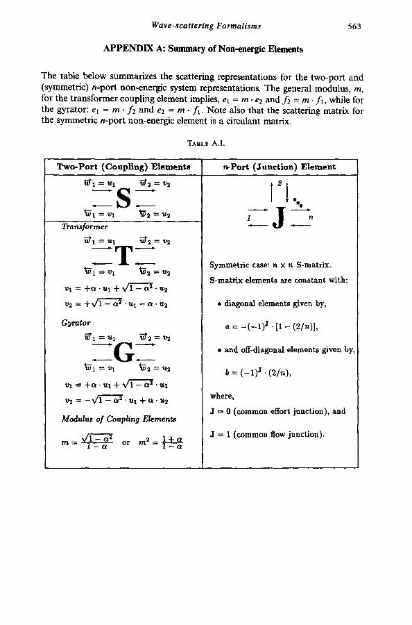
The table be low summar izes the scattering representat ions for the two-por t and (symmetr ic) n -por t non-energic system representations. The general modulus , m, for the t r a n s f o r m e r coupl ing e lement implies, el = m - e2 and f2 = m . f l , while for the gyra tor : el = m • f2 and e2 = m • f l . N o t e also that the scattering mat r ix for the symmet r i c n -por t non-energic element is a circulant matr ix .

TABLE A . I .

T w o - P o r t ( C o u p l i n g ) E l e m e n t s ~ P o r t ( J u n c t i o n ) E l e m e n t

iffl = Ul ~ff2 = v2

Transformer

iF1 = u l i f f2 = v2

T " ~ T = vl ti~2 = u2

v l = + ~ - ul + V ~ L - ' ~ • u2

v2 = +v~" - a2 • ul - a . u2

G y r a t o r

~F1 = u l i f f 2 = v2

G . " va = + ( ~ . u l + ~ f " L ' ~ . ~2

v2 = -1V'f'~'~- a a " u l + ~ . u2

M o d u l u s o f C o u p l i n g E l e m e n t s

1 ~ [ • %

.j q

Symmetric case: n X n S-matrix.

S-matr ix dements are constant with:

• diagonal elements given by,

a = - ( - 1 ) J . [1 - (2 /n) ] ,

• and off-diagonal elements given by,

b = (-x)J. (21,~),

where,

J = 0 (common effort junction), and

J --- 1 (common flow junction).

564 R. G. Longoria

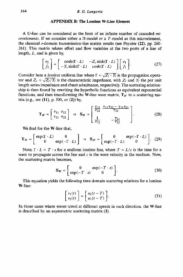
APPENDIX B: The Lossless W-Line Element

A U-line can be considered as the limit of an infinite number of cascaded mi- croelements. If we consider either a H-model or a T-model as this microelement, the classical s-domain transmission-line matrix results (see Paynter (22), pp. 260- 261). This matrix relates effort and flow variables at the two ports of a line of length, L, and is given by,

e2 cosh(F. L) -Z,,. sinh(F • L) ] [ / i ] (27)

Consider here a lossless uniform line where F = .]-~- I') is the propagation operator and Z~. = ~ is the characteristic impedance, with Z / a n d I') the per unit length series impedance and shunt admittance, respectively. The scattering relationship is then found by rewriting the hyperbolic functions as equivalent exponential functions, and then transforming the W-line wave matrix, Tw to a scattering matrix (e.g., see (11), p. 300, or (2)) by,

2--2T12 T2 I T w = [ T I I TI2] ~ Sw = . (28)

V21 T22 1 T__2. L T22 T22

We find for the W-line that,

0 e x p ( - F . L ) ~ S w = exp( .L) 0 "

Note, F • L = T • s for a uniform lossless line, where T --- L/c is the time for a wave to propagate across the line and c is the wave velocity in the medium. Now, the scattering matrix becomes,

[ 0 e x p ( - T , s) ] (30) Sw = e x p ( - T . s ) 0 "

This equation yields the following time domain scattering relations for a lossless W-line:

v2(t) = uj(t T) "

In those cases where waves travel at different speeds in each direction, the W-line is described by an asymmetric scattering matrix (2).

Documents

Wave-scattering Formalisms for Multiport Energetic Systems