Wave Breaking Velocity Effects in Depth-Integrated Models

8/4/2019 Wave Breaking Velocity Effects in Depth-Integrated Models

http://slidepdf.com/reader/full/wave-breaking-velocity-effects-in-depth-integrated-models 1/9

Wave breaking velocity effects in depth-integrated models

Patrick J. Lynett

Department of Civil Engineering, Texas A&M University, College Station, TX 77843-3136, United States

Received 11 May 2005; received in revised form 25 August 2005; accepted 12 October 2005

Available online 21 November 2005

Abstract

A simple model for predicting the velocities under breaking waves in depth-integrated models is developed. A velocity modification due towave breaking is formulated based on a specific exponential profile, which is then added to the numerically predicted, depth-integrated velocity

profile. This modification is superficial in that it does not directly change the hydrodynamic calculations inside the depth-integrated model. The

modifications can be employed in any of the numerous Boussinesq-type models, and is not dependant on the use of a particular breaking

dissipation scheme. Horizontal velocity profiles, both mean and instantaneous, are compared with experimental data in the surf zone. The

comparisons show good agreement, markedly better than the un-modified results, and on par with published numerical results from sophisticated

models.

D 2005 Elsevier B.V. All rights reserved.

Keywords: Boussinesq; Undertoe; Currents; Wave breaking

1. Introduction

For the near future, depth-integrated models will likely

dominate nearshore, wave-resolving simulation, in particular

when large spatial domains are considered. These models,

primarily the shallow water and Boussinesq-type variety,

predict the 3D wave field with 2D equations and so can

simulate large basins in a practical length of computational

time. While these properties seem to lead to great opportunities

for nearshore hydrodynamic predictions, the depth-integrated

derivation creates a set of equations for which some of the most

important nearshore physics are approximated, or left out

entirely.

Shallow-water-based depth-integrated models typically as-sume that the vertical profile of velocity can be represented by

a polynomial, wherein the order of the polynomial is

proportional to the accuracy of the resulting model. For non-

breaking waves, this polynomial predicts the vertical profile of

velocity very well, even for strongly nonlinear waves (e.g., Wei

et al., 1995; Ryu et al., 2003), provided the wave is not in deep

water. Implicit with this velocity profile, and often a direct

inviscid assumption, is a lack of ability to simulate turbulence.

To simulate nearshore hydrodynamics, some method must be

employed to approximate breaking, bottom friction, etc.The depth-integrated model, in general, consists of one

continuity equation, solved for the free surface elevation, and

one vector momentum equation, solved for some characteristic

velocity. To simulate the effects of breaking, the most common

approach is to add a dissipation submodel to the momentum

equation. This is an ad hoc addition, as common depth-

integrated derivations start with an inviscid assumption, either

implicitly or explicitly. There are two primarily classes of

breaking models: the roller model (e.g., Madsen et al., 1997)

and the eddy viscosity model (e.g., Kennedy et al., 2000). The

two models can be roughly equated, although the parameters

controlling the dissipations are based on different physicalthresholds.

Through a calibration of the parameters inherent in these

models, very good agreement in wave height and mean water

level can be achieved for wave transformation through the

surf zone. Due to the success in applying the Boussinesq-type

model through the surf, the natural progression is to employ

these models for transport calculations. Transport calculations

become very sensitive to accurate representation of the mean

horizontal velocity, or undertow if below the mean trough

level. It was immediately recognized that the raw Boussinesq

model yielded very poor predictions of this undertow. For

0378-3839/$ - see front matter D

2005 Elsevier B.V. All rights reserved.doi:10.1016/j.coastaleng.2005.10.020

E-mail address: [email protected].

Coastal Engineering 53 (2006) 325 – 333

www.elsevier.com/locate/coastaleng

http://dx.doi.org/doi:10.1016/j.coastaleng.2005.10.020





mailto:[email protected]


mailto:[email protected]



example, when using a Boussinesq-type model, here the two-

layer model of Lynett (in press), to predict the undertow of

the Cox et al. (1995) experiment, the results prove poor.

Shown in Fig. 1 are the numerical-experimental predictions.

The numerical profiles are the wave-averaged horizontal

velocities. As the numerical profiles are taken throughout

the water column, the undertow (below the trough) must be balanced by the crest flux (above the trough). This should be

the case with any finite amplitude wave theory — some

undertow must be predicted.

Shown in the subplots at x =3.5 m and x =5.8 m, the

numerical undertow agrees very well with the experimental.

The reason for this is that at these locations, breaking has not

yet initiated or has just barely initiated, and thus the impact on

the profile due to breaking is minimal. These two plots are

another demonstration of the ability of the Boussinesq model to

simulate nearshore hydrodynamics accurately. Looking to the

other four profiles shown, located throughout the surf zone, it

is clear that the undertow is not predicted correctly in either magnitude or vertical variation. The Boussinesq profiles are

always uniform below the trough, due to the Boussinesq-

interpreted long wave, inviscid nature of the breaking wave.

Using the ’’raw’’ Boussinesq velocity profiles to predict the

undertow leads to significant errors.

To work around this obstacle within the Boussinesq

framework, researchers have developed solutions across a

range of physical complexity. On the sophisticated end are the

approaches similar to Veeramony and Svendsen (2000), who

solved a coupled set of Boussinesq and vorticity models. Thisapproach does involve the inevitable vorticity generation

calibration, as well as a relatively complex equation model

(compared to the standard Boussinesq), but yields very good

agreement when compared to the undertow data of Cox et al.

(1995).

Much of the work in examining Boussinesq velocity profiles

in the surf zone employs the surface roller breaking model,

used with the improved Boussinesq equations of Madsen et al.

(1997). This particular model is somewhat limited in its ability

to predict the vertical profile of velocity due to the manipula-

tions of the model equations, rather than the velocity profile

used to derive said equations (e.g., Nwogu, 1993). Due to thesemanipulations, a velocity profile consistent with the solved

equations does not exist. However, in the surf zone, where

Boussinesq predicted velocities are close to uniform in the

Fig. 1. Comparison with the data of Cox et al. (1995). Top plot is the numerical wave height profile (line) and the experimental (circles). The bottom row of plots are

the time-averaged horizontal velocities at various locations, given in the subplot titles. The experimental values are shown with the dots, and the ‘‘unmodified’’Boussinesq results by the solid line.

P.J. Lynett / Coastal Engineering 53 (2006) 325–333326



vertical, this limitation will not impact the results greatly. When

using the roller breaking model, the horizontal velocity profile

under a breaking wave is modified such that in the roller

region, the velocity is assumed to be a large value related to the

local long wave speed, while the velocity under the roller is set

to a uniform value. This uniform value is determined such that

the modified flux is equal to the Boussinesq-predicted flux.While this approach has been shown to yield reasonable

results, it is not possible for this concept to predict a vertically

varying undertow, as is measured in many experiments,

without additional hydrodynamic submodels.

2. Breaker effect on depth-integrated velocity profile

A consistent modification to the velocity profile due to

breaking is sought. In its foundation, the procedure given in

this section is similar to the roller approach used to modify the

vertical velocity profile, discussed above. Here, however,

properties of the velocity modifications will be taken fromthe extended-Boussinesq theory.

Following the conventional perturbation derivation for

Boussinesq equations, the vertical profile of the vertical

velocity, W , is given in dimensionless form as:

W ¼ À zS À T þ O l2À Á

ð1Þ

where

S ¼ lIU ; T ¼ lI hU ð Þ; ð2Þ

z is the vertical coordinate, U is the vertically-varyinghorizontal velocity vector, and h is the local water depth. To

include the impact of breaking induced velocity profile

changes, a fundamental modification is made to the above

velocity profile:

W ¼ À zS À T þ A x; y; t ð Þ f x; y; z ; t ð Þ þ O l 2À Á

ð3Þ

where A and f comprise some arbitrary function which is meant

to approximately account for breaking effects. Using this

modified vertical velocity, the horizontal velocity vector, as

referenced to a velocity at an arbitrary elevation, is given by:

U ¼ u À l2 z 2 À z 2a

2lS þ z À z

að ÞlT

'&

þ l 2 l A

Z f z ð Þdz À

Z f z

að Þdz

!&

þ A

Z l f z ð Þdz À

Z l f z að Þdz

! 'þ O l4

À Áð4Þ

where u is the horizontal velocity evaluated at some arbitrary

elevation z a

. The purpose of the additional terms in the

horizontal velocity profile will be to allow velocities near the

free surface to be larger when breaking is occurring, to better

represent the fast moving breaking region. It is desired that

U ( x, y,f,t ) =C ( x, y,t ) where C is some prescribed free surface

breaking velocity and f is the free surface elevation. Further,

let us define the Boussinesq predicted free surface velocity

us ¼ u À l2 f2 À z 2a

2lS þ f À z

að ÞlT

'&þ O l4

À Á: ð5Þ

Therefore, a solution to the following expression is desired:

l 2l A

Z f fð Þdz À

Z f z

að Þdz

!

þ l 2 A

Z l f fð Þdz À

Z l f z

að Þdz

!¼ C À us ð6Þ

Using the assumption that l f ( z ) = O(l2), employing f ( z a

) =

f ( z B) + O(l2) where z B is some elevation in the water column,

and the substitution g = X f d z , a relatively simple equations

results

g fð Þ À g z Bð Þ ¼ 1 ð7Þ

where l A has been set equal to dl 2 C À usð Þ; and d=1 when

breaking is occurring and is 0 otherwise. As the initial

modifications to the vertical velocity profile are ad hoc in

nature, there is no guidance contained directly in the depth-

integrated derivation as to what form g ( z ) should take. Since

the Boussinesq-model should capture the velocities correctly

if the phenomenon is of the shallow- or intermediate-water

type, we chose here to give g a deep-water based form, an

exponential:

g ¼ Be k z Àfð Þ ð8Þ

where B is a coefficient and k is some vertical wave number.

Substituting this form into (7) gives the solution for B:

B ¼1

1 À e k z BÀfð Þð9Þ

and we are left with the wave number, k , and the elevation,

z B, as unknowns. From this point on, all terms will be

discussed in their dimensional form. To summarize, the

modified horizontal velocity profile is given as:

U ¼ U O þ U B ð10Þ

where

U O ¼ u Àz 2 À z 2

a

2lS þ z À z

að ÞlT

'&ð11Þ

U B ¼ l A g z ð Þ À g z Bð Þ½ � ð12Þ

l A ¼ d C À usð Þ ð13Þ

It is noted that (10) is written in a more generic form using

U O. While the derivation up to this point has looked at the

‘‘extended’’ Boussinesq model, it is completely applicable to

any Boussinesq-type of model, for example depth-averaged

or multi-layer. In these cases, only the expression for U O in

(11) would change.

P.J. Lynett / Coastal Engineering 53 (2006) 325–333 327



With any modification of the velocity profiles comes a

modification to the resulting depth-integrated continuity and

momentum equations. The additional flux terms in thecontinuity equation areZ f

Àh

l A g z ð Þ À g z Bð Þ½ �dz

¼ Bl A1

k 1 À eÀk H À Á

À H e k z BÀfð Þ

!ð14Þ

where H =f + h. Now, to solve the continuity equation, some

value for k must be given. There are a few possibilities here, for

example, k can be related somehow to the total water depth, i.e.,

k = 2k / H , or based on some other instantaneous wave property,

i.e., k ¼ ffiffiffiffiffiffiffiffiffiffiffiffiffi

jf xx=fjp

where x is the direction of propagation of the breaker. A value of k will be chosen that yields good agreement

with experiment — it will be the empirical parameter of the

breaking velocity modifications. With a given k , we are left with

z B as the remaining unspecified variable. Here, a choice is made

for z B based on experience when using the Boussinesq model

for breaking wave studies. It is seen that the ‘‘unmodified’’

model, when using either a roller or eddy–viscosity breaker

submodel in the momentum equation, reproduces mean

quantities (wave height, mean free surface, etc.) in the surf

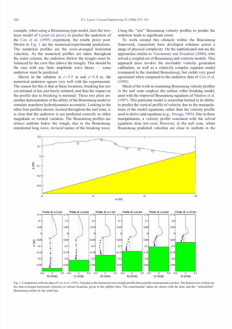
Fig. 2. Horizontal velocity modifications due to breaking, where the line with open circles is for f =0.3 h, the dashed line for f =0.2 h, the solid line for f =0, the

dashed–dotted line for f = À0.1 h, and the solid dotted line for f = À0.2 h.

Fig. 3. Comparison with the data of Cox et al. (1995), using the same setup as in Fig. 1. The experimental values are shown with the dots, the breaking-enhancedBoussinesq by the solid line, and the unmodified Boussinesq results by the dashed–dotted line.




accurately. Thus the flux predicted by the ‘‘unmodified’’ model

is already well predicted. We will chose z B such that the new

terms do not change the flux, i.e.,

Z fÀh

l A g z ð Þ À g z Bð Þ½ �dz ¼ 0 ð15Þ

or

eÀkH þ kH e k z BÀfð Þ ¼ 1 ð16Þ

The above equation is readily solved for z B:

z B ¼ À h þln½ 1

kH ðe kH À 1Þ�

k ð17Þ

Therefore, with a specified value of k , z B is given and the

breaking modifications to the velocity profile in (10) can be

calculated. In the limit of very small k (long wave), the

modifications resemble a linear trend going from a velocityaddition at the free surface to a velocity subtraction near the

bed, with z B approaching À h + H /2, the midpoint of the

instantaneous water column. For large k , the modification is a

velocity addition highly localized at the surface and a small

velocity subtraction in the remaining water column, with z Bapproaching f.

Looking to the momentum equation, additional terms will

also be present when carrying through the modified velocity

profiles. The assumption is made that the breaking submodels

have already taken these terms in account in some approximateform. Thus, it can be concluded that the modifications given by

(10) are in fact the implied velocity profile changes associated

with the use of a breaking submodel, here the eddy viscosity

model. In addition, since the changes presented here do not

affect the governing equations, all previous free surface

benchmarks and calibrations remain unchanged, and, in

essence, the velocity profile changes in (10) are a post-

processing modification.

3. Comparison with experimental data

The modified velocity profile under breaking waves will becompared with the available experimental data in this section.

The data of Cox et al. (1995) and Ting and Kirby (1995, 1996),

for both mean flows (undertoe) and phase-averaged velocities,

Fig. 4. Comparison with the data of Ting and Kirby spiller. The top plot shows the mean crest level (stars), mean water level (triangles), and mean trough level

(circles) for the experiment as well as the numerical simulation. The lower subplots are the time-averaged horizontal velocities, where the experimental values areshown with the dots, the breaking-enhanced Boussinesq by the solid line, and the unmodified Boussinesq results by the dashed–dotted line.




is used. To achieve the best possible agreement with the data,

the following value of k is specified:

k ¼5

H ð18Þ

The solutions are not strongly sensitive to this choice, with

numerator values ranging from 4 to 6 yielding similar results. Note that the numerator value, as well as the chosen form of k ,

are chosen based on the model employed here, and may be

different for other Boussinesq-type models. To elucidate how

the added terms to (10) will modify the profile, Fig. 2 gives U Bfor various free surface elevation values. At the free surface, an

addition is made such that the velocity is equal to C , where

C ¼us

jusj

ffiffiffiffiffiffiffiffiffiffiffiffiffiffiffiffiffiffiffiffiffigravity4 H

p þ U

;

; ð19Þ

the nonlinear long wave speed corrected for the depth-averaged

current, U ¯ . Downward through the water column, the velocity

addition decreases until the modifications act to reduce thevelocity. Note that these curves will collapse if plotted against

( z Àf) / H instead of z / h, following the f =0 curve given in

Fig. 2.

For the Boussinesq simulations, the highly-nonlinear,

extended Boussinesq model is used for all simulations. A

close variation of the eddy–viscosity model is employed to

approximate wave breaking, as described in Lynett (in press).

As a first experimental comparison, the data of Cox et al.

(1995) is examined. Remember that this data has already been

compared with the ’’unmodified’’ model, as shown in Fig. 1.The unmodified model, while capturing the mean velocity

correctly near the trough level, shows significant errors below

the trough. With the breaking velocity ‘‘enhancements’’, the

mean velocities are predicted very well, as shown in Fig. 3.

Both the magnitude and the vertical variation of undertow are

captured throughout the surf zone. For this case, the breaking

enhancements are large, leading to big differences in the two

results, and indicating that for this wave, the Boussinesq

predicted free surface velocity is much less than the nonlinear

long wave speed. The agreement shown here is on par with

published comparisons, based on more physically robust and

computationally expensive formulations (e.g., Veeramony andSvendsen, 2000).

Next, the data of Ting and Kirby, for spilling (1995) and

plunging (1996) breakers, is compared. These experiments

Fig. 5. Comparison with the data of Ting and Kirby plunger. The top plot shows the mean crest level (stars), mean water level (triangles), and mean trough level

(circles) for the experiment as well as the numerical simulation. The lower subplots are the time-averaged horizontal velocities, where the experimental values are

shown with the dots, the breaking-enhanced Boussinesq by the solid line, and the results of a VOF RANS model (COBRAS, provided by Dr. P. Lin) by thedashed line.




Fig. 6. Comparisons of the vertical profile of phase-averaged horizontal velocity at different wave phases for the Ting and Kirby spiller at x =7.2 m. The top plot

shows the experimental phase-averaged free surface. In the lower subplots are the velocity profiles at different points under the wave, where the dots are the

experiment, the breaking-enhanced Boussinesq by the solid line, and the unmodified Boussinesq results by the dashed line. Velocity in the lower plots is scaled by co,

the linear long wave speed.

Fig. 7. Comparisons of the vertical profile of phase-averaged horizontal velocity at different wave phases for the Ting and Kirby spiller at x =7.8 m. Figure setupsame as Fig. 6.




look at cnoidal wave breaking on a 1/35 slope. First, mean

velocity profiles are discussed. In Fig. 4 are comparisons at

four locations along the slope. As with the Cox et al. data,

velocity measurements below the trough are available. The

breaking enhanced model does a much better job at represent-

ing the undertow profile, including the vertical variation. The

agreement at x = 8.4 m is poor, although equal to the agreement achieved in other models (e.g., Lin and Liu, 2004). As with the

data of Cox et al., the breaking enhanced model predicts a very

different undertow profile as compared to the unmodified

model.

A physical setup that does not show much difference

between the breaking enhanced and unmodified models is that

of Ting and Kirby (1996) for plunging cnoidal waves. For this

comparison, shown in Fig. 5, the breaking enhanced model is

compared with the experimental and the numerical results from

a RANS VOF model, COBRAS (Lin and Liu, 1998). Before

breaking, at x =6.3 m, the predictions of the two numerical

models through the entire water column are in agreement. Inthe outer surf zone, the RANS model predicts the undertow

better, capturing the vertical variation. Also note that at these

locations, the positive mass flux, above the trough level, as

predicted by the two models are in very close agreement.

Moving towards the inner surf, the Boussinesq breaking

enhanced model yields a much better prediction of the

undertow, with excellent agreement at the two innermost

measurement locations. The breaking enhanced impact for this

case is in fact rather small, as can be inferred from the small

vertical variation of the undertow predicted by this model. This

implies that the Boussinesq prediction of the free surface

velocity of the breaker is near the nonlinear long wave speed.

While examination of the undertow profiles indicates that

the breaking enhancements are correctly modifying the velocity

profiles in the mean sense, it does not necessary require that the

instantaneous profiles are being altered reasonably. To inves-

tigate this point, the data of Ting and Kirby (1995), for thespiller, is re-examined. The experimental velocity profiles are

phase-averaged, which is the equivalent of the instantaneous

Boussinesq velocity profile, where turbulent fluctuations are

not modelled. Figs. 6–8 give comparisons at three locations,

x =7.2, 7.8, and 9 m, respectively. In the top plot of each of

these figures is the free surface elevation (waveform) for one

wave period.

Looking to the vertical profiles of horizontal velocity, given

in the lower subplots of the figures, it becomes clear that while

the breaking enhancements have been shown to predict

undertow well, they also capture the phase-averaged velocities

below the mean trough level. Given in each figure are three profiles under the breaking part of the wave, and two

elsewhere. Note that the unmodified profiles are close to

vertically invariant at all locations under the wave. Only at the

trough of the wave, however, is this a good approximation.

The breaking enhancements show a large improvement over

the unmodified predictions, with the vertical variation and the

velocity magnitude very well modelled. It is also evident that

below the trough level, the proposed modification will act to

reduce the horizontal velocity under the breaker, thereby

generally decreasing the skewness (and asymmetry) of the

Fig. 8. Comparisons of the vertical profile of phase-averaged horizontal velocity at different wave phases for the Ting and Kirby spiller at x =9.0 m. Figure setupsame as Fig. 6.




under-trough velocity. The effect is opposite above the trough.

This incorrect under-trough prediction in the unmodified

Boussinesq model has been recognized previously; for

example see the ‘‘roller’’ velocity modification in some

Boussinesq models (commonly in the Madsen et al. (1997)

type Boussinesq models, see developments by Rakha (1998)).

To reiterate, the unmodified Boussinesq model is capturing thedepth-averaged velocity well at all locations — but the vertical

variation is missing under the breaking portion. This observa-

tion served as the spark for the research presented here.

4. Conclusions

A simple model for predicting the velocities under breaking

waves in depth-integrated models is developed. Under the non-

breaking portions of the wave, no modification is made to the

Boussinesq vertical profiles of velocity. The velocity modifi-

cation is formulated based on a specific exponential profile,

which is then added to the numerically predicted velocity profile under a breaking wave. This modification is superficial

in that it does not directly change any of the hydrodynamic

calculations inside the depth-integrated model. However, if one

were to employ these modifications in a model that used the

velocity for transport predictions through the surf and swash,

the predictions would be different. The modifications can be

employed in any of the numerous Boussinesq-type models, and

is not dependant on the use of any of the existing breaking

dissipation schemes. It is reiterated here that much of the

benefit of this ‘‘breaking enhancement’’ comes from its

simplicity and ability to be seamlessly integrated into existing

models.

While the established experimental data with which tocompare these modifications is limited, the results are

promising in both the average and instantaneous sense. The

approach presented here could be extended to the boundary

layer as well, or, alteratively, one could use a more physically

detailed approach (e.g., Liu and Orfila, 2004). Extension of this

approach to 2HD is also straightforward, although additional

and ongoing research into the inclusion of vertical vorticity

evolution is equally important for velocity profile modeling.

With accurate velocity profiles both in magnitude and vertical

variation, such as those given here, using established Boussi-

nesq-type models, without additional viscous sub-models, to

simulate transport in the surf zone becomes a more promising

endeavor.

Acknowledgement

The research presented here was partially supported by a

grant from the National Science Foundation (CTS-0427115).

References

Cox, D.T., Kobayashi, N., Okayasu, A., 1995. Experimental and numerical

modeling of surf zone hydrodynamics. Technical Report CACR-95-07.

Center for Applied Coastal Research, University of Delaware.

Kennedy, A.B, Chen, Q., Kirby, J.T., Dalrymple, R.A., 2000. Boussinesq

modeling of wave transformation, breaking and runup: I. One dimension.

Journal of Waterway, Port, Coastal, and Ocean Engineering 126, 39–47.

Lin, P., Liu, P.L.-F., 1998. A numerical study of breaking waves in the surf

zone. Journal of Fluid Mechanics 359, 239–264.

Lin, P., Liu, P.L.-F., 2004. Discussion of vertical variation of the flow across the

surf zone. Coastal Engineering 50, 161–164.

Liu, P.L.-F., Orfila, 2004. Viscous effects on transient long wave propagation.

Journal of Fluid Mechanics 520, 83– 92.

Lynett, P., in press. Nearshore wave modeling with high-order Boussinesq-type

equations. Journal of Waterway, Port, Coastal and Ocean Engng.

Madsen, P.A., Sorensen, O.R., Schaffer, H.A., 1997. Surf zone dynamics

simulated by a Boussinesq-type model. Part I. Model description and cross-

shore motion of regular waves. Coastal Engineering 32, 255–287.

Nwogu, O., 1993. Alternative form of Boussinesq equations for nearshore wave

propagation. Journal of Waterway, Port, Coastal, and Ocean Engineering

119 (6), 618–638.

Rakha, K.A., 1998. A quasi-3D phase-resolving hydrodynamic and sediment

transport model. Coastal Engineering 34, 277– 311.

Ryu, S., Kim, M.H., Lynett, P., 2003. Fully nonlinear wave– current

interactions and kinematics by a BEM-based numerical wave tank.

Computational Mechanics 32, 336–346.

Ting, F.C.-K., Kirby, J.T., 1995. Dynamics of surf-zone turbulence in a strong

plunging breaker. Coastal Engineering 24, 177 – 204.

Ting, F.C.K., Kirby, J.T., 1996. Dynamics of surf-zone turbulence in a spilling

breaker. Coastal Engineering 27, 131 – 160.

Veeramony, J., Svendsen, I., 2000. The flow in surf zone waves. Coastal

Engineering 39, 93– 122.

Wei, G., Kirby, J.T., Grilli, S.T., Subramanya, R., 1995. A fully nonlinear

Boussinesq model for surface waves: Part 1. Highly nonlinear unsteady

waves. Journal of Fluid Mechanics 294, 71– 92.


Documents

Wave Breaking Velocity Effects in Depth-Integrated Models