WAVE BACKSCATTERING BY POINT …ksolna/research/92scatt.pdfwave backscattering by point scatterers in the random paraxial regime josselin garnier and knut s˜lnay and knut s˜lnayPublished

WAVE BACKSCATTERING BY POINT SCATTERERS IN THERANDOM PARAXIAL REGIME

JOSSELIN GARNIER∗ AND KNUT SØLNA†

Abstract. When waves penetrate a medium without coherent reflectors, but with some finescale medium heterogeneities, the backscattered wave is incoherent without any specific arrival timeor the like. In this paper we consider a distributed field of microscatterers, like aerosols in theatmosphere, which coexists with microstructured clutter in the medium, like the fluctuations of theindex of refraction of the turbulent atmosphere. We analyze the Wigner transform or the angularlyresolved intensity profile of the backscattered wave when the incident wave is a beam in the paraxialregime. An enhanced backscattering phenomenon is proved and the properties of the enhancedbackscattering cone (relative amplitude and profile) are shown to depend on the statistical parametersof the microstructure, but not on the microscatterers. These results are based on a multiscale analysisof the fourth-order moment of the fundamental solution of the white-noise paraxial wave equation.They pave the way for an estimation method of the statistical parameters of the microstructurefrom the observation of the enhanced backscattering cone. In our scaling argument we differentiatethe two important canonical scaling regimes which are the scintillation regime and the spot dancingregime.

Key words. Waves in random media, parabolic approximation, scintillation, enhanced backscat-tering, turbulence estimation.

AMS subject classifications. 60H15, 35R60, 74J20.

1. Introduction. In this paper we consider the propagation of a beam in aturbulent medium in which imbedded particles play the role of point scatterers. Theseparticles can be dust and aerosols in the turbulent atmosphere for instance. Weconsider the case in which the particles occupy an extended region and their densityis invariant in the transverse direction (at least transversally invariant in the regionilluminated by the incoming beam). The particles scatter light in all directions but weare only interested in the light that is backscattered and that can be collected in thesame plane as the original source. The backscattering phenomena which are studiedin this paper relate to single scattering from the particles imbedded in the turbulentmedium and to complex interaction with the turbulent medium itself.

Our main goal is to study the dependence of the backscattered light with respectto the statistics of the random turbulent medium. The particle cloud plays the role ofan uncontrolled source of backscattered light. We show that the mean backscatteredintensity spatial profile does not depend on the statistical properties of the turbulentmedium, but the covariance function of the backscattered waves, or equivalently theWigner transform, depends on the statistical properties of the turbulent medium. Inparticular, by looking at the angular distribution of the backscattered energy flux,it is possible to exhibit an enhanced backscattering phenomenon and to relate thewidth of the enhanced backscattering cone and the enhancement factor to statisticalparameters of the turbulent medium such as the Hurst exponent.

Enhanced backscattering or weak localization has been extensively discussed inthe physical literature [3, 33] and observed in several experimental contexts [35, 32,29, 22]. It usually refers to the situation that the mean backscattered power for aquasi-monochromatic quasi-plane has a local maximum in the backscattered direction,

1Laboratoire de Probabilites et Modeles Aleatoires & Laboratoire Jacques-Louis Lions, UniversiteParis Diderot, 75205 Paris Cedex 13, France [email protected]

2Department of Mathematics, University of California, Irvine CA 92697 [email protected]

1

2 J. Garnier and K. Sølna

which is twice as large as the mean backscattered power in the other directions. Theclassical enhanced backscattering phenomenon happens in a regime of multiple scat-tering by point scatterers and it results from the constructive interference of reciprocallight paths. In our paper we address a regime in which the waves experience singlescattering by the point scatterers and the interaction of the waves with the turbulentmedium is responsible for the enhanced backscattering phenomenon. Therefore, theproperties of the cone depend on the statistical properties of the turbulent mediumand not on the distribution of point scatterers.

In our paper the propagation through the turbulent medium is described by anIto-Schrodinger equation [6]. This model is natural in many situations where a beampropagates mostly in the forward direction and the correlation length of the mediumis much smaller than the propagation distance [4, 8, 9, 15, 25, 26, 27]. It allows forthe use of Ito’s stochastic calculus, which in turn enables the closure of the hierar-chy of moment equations and the statistical analysis of important wave propagationproblems, such as scintillation [2, 10, 12, 18, 30, 31, 34, 36] and in various appli-cations to imaging and communication [1]. The analysis of the mean intensity andthe Wigner transform of the backscattered wave involves fourth-order moments ofthe Green’s function of the Ito-Schrodinger equation. The main theoretical result ofthis paper is a multiscale analysis of the fourth-order moments of the solution of theIto-Schrodinger equation. This multiscale analysis allows to capture and characterizecompletely the narrow enhanced backscattering cone in the situation described above.

The paper is organized as follows. We briefly review the white-noise paraxialmodel in Section 2. We derive an integral representation of the covariance functionof the backscattered field in Section 3, which shows that the fourth-order momentsof the fundamental solutions are needed. We review the general moment equationsin Section 4. We introduce two possible propagation regimes in Section 5 and westudy the asymptotics of the covariance function of the backscattered field in thesetwo regimes in Section 7. We give closed-form expressions for the Wigner distributionof the backscattered field in Section 8 and discuss the dependence of the enhancedbackscattering cone with respect to the statistics of the random medium. Finallywe carry out a few numerical simulations to illustrate the theoretical predictions inSection 9.

2. The White-Noise Paraxial Model. Let us consider the time-harmonicwave equation with homogeneous wavenumber k0, random index of refraction n(z,x),and source in the plane z = zi:

∆u+ k20n2(z,x)u = −δ(z − zi)f(x). (2.1)

Denote by λ0 the carrier wavelength (equal to 2π/k0), by L the typical propagationdistance, and by r0 the radius of the initial transverse beam/source. The paraxialregime holds when the wavelength λ0 is much smaller than the radius r0, and when thepropagation distance is at most of order r20/λ0 (the so-called Rayleigh length). Thewhite-noise paraxial regime that we address in this paper holds when, additionally,the index of refraction of the medium has random fluctuations with a small typicalamplitude and with correlation length much larger than the wavelength but smallerthan the propagation distance. We refer to [16] for the explicit scaling assumptions. Inthis regime the solution of the time-harmonic wave equation (2.1) can be approximatedby

u(z,x) =i

2k0

∫f(xi)G((zi,xi), (z,x))dxi exp

(ik0|z − zi|

),

Wave backscattering by point scatterers in the random paraxial regime 3

where (G((zi,xi), (z,x)))z∈R,x∈R2 is the paraxial fundamental solution of the Ito-Schrodinger equation

dG(z,x) =i

2k0∆xG(z,x)dz +

ik02G(z,x) ◦ dB(z,x), (2.2)

with the initial condition in the plane z = zi:

G((zi,xi), (z = zi,x)) = δ(x− xi).

Here the symbol ◦ stands for the Stratonovich stochastic integral and B(z,x) is areal-valued Brownian field over R× R2 with covariance

E[B(z,x)B(z′,x′)] = min{|z|, |z′|}C(x− x′), (2.3)

assuming zz′ > 0. The model (2.2) can be obtained from the scalar wave equation(2.1) by a separation of scales technique in which the three-dimensional fluctuations ofthe index of refraction n(z,x) are described by a zero-mean stationary random processν(z,x) with mixing properties: n2(z,x) = 1 + ν(z,x). The covariance function C(x)in (2.3) is then given in terms of the two-point statistics of the random process ν by

C(x) =

∫ ∞−∞

E[ν(z′ + z,x′ + x)ν(z′,x′)]dz. (2.4)

The covariance function C is assumed to decay fast enough at infinity so that itbelongs to L1(R2). Its Fourier transform is nonnegative (since it is the power spectraldensity of the stationary process x → B(1,x)). The white-noise paraxial model iswidely used in the physical literature [1]. It simplifies the full wave equation (2.1)by replacing it with an initial value-problem (2.2). It was studied mathematically in[6]. The proof of its derivation from the three-dimensional wave equation in randomlyscattering medium uses tools presented in [11] and it is given in [16].

3. The Backscattered Field. We assume a Gaussian source in the plane z = 0with radius r0 emitting toward z < 0:

f(x) = exp(− |x|

2

2r20

).

We assume that there is a Poisson cloud (or Poisson point process [21]) giving pointscatterers in the medium for z < 0:

n2ps(z,x) =∑j

wjδ(x− xj)δ(z − zj).

The time-harmonic field satisfies

∆u+ k20[n2(z,x) + n2ps(z,x)]u = −δ(z)f(x).

Using the Born (or single-scattering) approximation for the point scatterers, thebackscattered field recorded in the plane z = 0 at (0,xr) is

u(0,xr) = −1

4

∑j

exp(2ik0|zj |

) ∫dx0f(x0)G((0,x0), (zj ,xj))wjG((zj ,xj), (0,xr)).

(3.1)


The use of the paraxial fundamental solution G is justified because the point scatterersplaying the roles of secondary sources are along the z-axis (in a tube that is illuminatedby the incident beam) and the field is collected in the plane z = 0 but close to thez-axis as well.

In this paper we assume that the intensity ρps(z) of the Poisson cloud dependsonly on z. In practice our results can be extended to the case when the intensityof the Poisson cloud varies laterally on a scale that is slow relative to the beamwidth. It is assumed to be supported in the region z < 0 away from 0. The scale ofvariation of the function ρps(z) is assumed to be much larger than the wavelength.The reflectivities wj of the scatterers can be deterministic or random, we denote byσ2 their second moment and by w their first moment. In this configuration the meanof the backscattered field is:⟨

u(0,xr)⟩

= − w4

∫ 0

−∞dziρps(zi) exp

(− 2ik0zi

) ∫dxi

∫dx0f(x0)

×G((0,x0), (zi,xi))G((zi,xi), (0,xr)), (3.2)

where 〈·〉 stands for the expectation with respect to the distribution of the pointscatterers. This equation follows from the general result that, for a Poisson pointprocess with intensity ρ(z,x), we have for any test function g(z,x) [21, Eq. (3.9)]:⟨∑

j

g(zj ,xj)⟩

=

∫g(z,x)ρ(z,x)dzdx.

The presence of the rapid phase exp(−2ik0zi) in (3.2) averages out the integral tozero, which shows that the backscattered field has mean zero:⟨

u(0,xr)⟩

= 0. (3.3)

This result means that the backscattered wave is incoherent. The covariance functionof the backscattered field is our main quantity of interest:

⟨u(0,xr)u(0,x′r)

⟩=σ2

16

∫ 0

−∞dziρps(zi)

∫dxi

∫∫dx0dx

′0f(x0)f(x′0)

×G((0,x0), (zi,xi))G((zi,xi), (0,xr))G((0,x′0), (zi,xi))G((zi,xi), (0,x′r)).

This equation follows from the general result that, for a Poisson point process withintensity ρ(z,x), we have for any test function g(z,x) [21, Eq. (3.10)]:⟨∣∣∑

j

g(zj ,xj)∣∣2⟩ =

∫|g(z,x)|2ρ(z,x)dzdx+

∣∣∣ ∫ g(z,x)ρ(z,x)dzdx∣∣∣2.

Using reciprocity we have

G((0,x0), (zi,xi)) = G((zi,xi), (0,x0)) and G((0,x′0), (zi,xi)) = G((zi,xi), (0,x′0)).

Therefore,

⟨u(0,xr)u(0,x′r)

⟩=σ2

16

∫ 0

−∞dziρps(zi)

∫dxi

∫∫dx0dx

′0f(x0)f(x′0)

×G((zi,xi), (0,x0))G((zi,xi), (0,xr))G((zi,xi), (0,x′0))G((zi,xi), (0,x′r)).


Using the statistical homogeneity of the random medium we have in distribution (withrespect to the distribution of the random medium) for any zi < 0:

(G((zi,xi), (0,x)))x∈R2dist.= (G((0,xi), (|zi|,x)))x∈R2 .

Therefore, by taking the expectation with respect to the distribution of the pointscatterers and the distribution of the random medium, we have

E[u(0,xr)u(0,x′r)] =σ2

16

∫ ∞0

dzρ(z)

∫dxi

∫∫dx0dx

′0f(x0)f(x′0)

×E[G((0,xi), (z,x0))G((0,xi), (z,xr))G((0,xi), (z,x′0))G((0,xi), (z,x′r))

], (3.4)

where ρ(z) = ρps(−z). This equation shows that we need to compute the fourth-ordermoment of the paraxial fundamental solution. In fact we only need to compute theintegral over xi of this quantity, which is in fact simpler.

If the source is not time-harmonic, but a pulse with carrier frequency ω0 that isemitted at time 0, and if the recorded wave is time-windowed within the time-interval[T1, T2], then the time integrated covariance function of the backscattered wave

1

(2π)2

∫ T2

T1

E[u(t, 0,xr)u(t, 0,x′r)]dt

is given by an integral of type (3.4) where k0 = ω0/c0 is the carrier wavenumber(with c0 the background wave speed) and the integral in z is essentially limited to[z1, z2] with zj = c0Tj/2. Note that, if the pulse is broadband in the sense that thebandwidth is of the same order as the carrier frequency, then we need to integrate(3.4) over the bandwidth. We will only consider narrowband pulses in our paper.This time-windowing technique is a practical way to select the propagation distancethat is probed by the reflection method.

4. The General Moment Equations. The main tool for describing wavestatistics are the finite-order moments. We show in this section that in the con-text of the Ito-Schrodinger equation (2.2) the moments of the field satisfy a closedsystem at each order [20, 12]. For xi ∈ R2, p ∈ N, we define

M (p)xi

(z, (xj)

pj=1, (yl)

pl=1

)= E

[ p∏j=1

G((0,xi), (z,xj))

p∏l=1

G((0,xi), (z,yl))], (4.1)

for (xj)pj=1, (yl)

pl=1 ∈ R2p. Using the stochastic equation (2.2) and Ito’s formula

for Hilbert space valued processes [24], we find that the function M(p)xi satisfies the

Schrodinger-type system:

∂M(p)xi

∂z=

i

2k0

( p∑j=1

∆xj−

p∑l=1

∆yl

)M (p)xi

+k204Up((xj)

pj=1, (yl)

pl=1

)M (p)xi, (4.2)

M (p)xi

(z = 0) =

p∏j=1

δ(xj − xi)

p∏l=1

δ(yl − xi), (4.3)


with the generalized potential

Up((xj)

pj=1, (yl)

pl=1

)=

p∑j,l=1

C(xj − yl)−1

2

p∑j,j′=1

C(xj − xj′)−1

2

p∑l,l′=1

C(yl − yl′)

=

p∑j,l=1

C(xj − yl)−∑

1≤j<j′≤p

C(xj − xj′)−∑

1≤l<l′≤p

C(yl − yl′)− pC(0). (4.4)

We introduce the Fourier transform

M (p)xi

(z, (ξj)

pj=1, (ζl)

pl=1

)=

∫∫M (p)xi

(z, (xj)

pj=1, (yl)

pl=1

)× exp

(− i

p∑j=1

xj · ξj + i

p∑l=1

yl · ζl)dx1 · · · dxpdy1 · · · dyp. (4.5)

It satisfies

∂M(p)xi

∂z= − i

2k0

( p∑j=1

|ξj |2 −p∑l=1

|ζl|2)M (p)xi

+k204UpM (p)

xi, (4.6)

M (p)xi

(z = 0) = exp(− i

p∑j=1

xi · ξj + i

p∑l=1

xi · ζl). (4.7)

In Eq. (4.6) the operator Up is defined by

UpM (p)xi

=1

(2π)2

∫C(k)

[ p∑j,l=1

M (p)xi

(ξj − k, ζl − k)−∑

1≤j<j′≤p

M (p)xi

(ξj − k, ξj′ + k)

−∑

1≤l<l′≤p

M (p)xi

(ζl − k, ζl′ + k)− pM (p)xi

]dk, (4.8)

where we only write the arguments that are shifted. It turns out that the equation

(4.6) for the Fourier transform M(p)xi is easier to solve than (4.2). In particular it can

be integrated readily if the medium is homogeneous.

5. Regimes of Propagation. In order to get closed-form expressions for somerelevant quantities, we will address the two following particular regimes, which canbe considered as particular cases of the paraxial white-noise regime. Let us denoteby ϑ the standard deviation of the fluctuations of the index of refraction and by lz(resp. lx) the longitudinal (resp. transverse) correlation length of the fluctuationsof the index of refraction. Then the correlation length in the propagation direction,C(0), is of order ϑ2lz and the transverse scale of variation of C(x) is of order lx. Asbefore, λ0 is the carrier wavelength (equal to 2π/k0), L is the typical propagationdistance, and r0 is the radius of the initial transverse beam/source. In this notationthe Rayleigh length, which corresponds to the distance when the transverse radiusof the beam roughly has doubled by diffraction in the homogeneous medium case, isr20/λ0. Moreover, as seen in (4.2) k20C(0)L or ϑ2lzL/λ

20 is a measure of the relative

strength of the medium fluctuations over the propagation distance. In what follows,ε is a small dimensionless parameter.


• The spot-dancing regime. The random medium fluctuations are relativelystrong, so that ϑ2lzL/λ

20 is of order 1/ε2, the initial beam support is small, so

that r0/lx is of order ε, and the propagation distance is such that Lλ0/r20 is of

order one (ie the typical propagation distance is of the order of the Rayleighlength of the initial beam). This leads to a picture where the transmittedwave field center “dances” according to a random frame [6, 18].

• The scintillation regime. The random medium fluctuations are relativelyweak, so that ϑ2lzL/λ

20 is of order one, the initial beam support is broad, so

that r0/lx is of order 1/ε, while the propagation distance is such that Lλ0/r20

is of order 1/ε (ie the typical propagation distance is relatively large comparedto the Rayleigh length of the initial beam). This leads to a picture consistentwith random and Gaussian fluctuations for the transmitted field [18].

5.1. The Spot-Dancing Regime. In this subsection we review the results thatcan be found in [1, 6, 13, 14] and put them in a convenient form for the forthcominganalysis. In this regime the covariance function Cε is of the form:

Cε(x) = ε−2C(εx), (5.1)

for a small dimensionless parameter ε. We want to study the asymptotic behavior ofthe moments of the field in this regime, that we call spot-dancing regime for reasonsthat will become clear in the analysis.

In the spot-dancing regime we assume that the power spectral density C(k) decaysfast enough so that

∫|k|4C(k)dk is finite. This implies that the covariance function

C(x) is at least four times differentiable at x = 0, which corresponds to a smoothrandom medium. For simplicity, we also assume that the random fluctuations areisotropic in the transverse directions, in the sense that the covariance function C(x)depends only on |x|. We denote

γ =1

2(2π)2

∫|k|2C(k)dk = −1

2∆C(0). (5.2)

The operator Uεp has then the form

UεpM (p)xi

=ε−2

(2π)2

∫C(k)

[ p∑j,l=1

M (p)xi

(ξj − εk, ζl − εk)

−∑

1≤j<j′≤p

M (p)xi

(ξj − εk, ξj′ + εk)

−∑

1≤l<l′≤p

M (p)xi

(ζl − εk, ζl′ + εk)− pM (p)xi

]dk, (5.3)

and it can be expanded as ε→ 0 as

UεpM (p)xi

=γ

2

( p∑j=1

∇ξj +

p∑l=1

∇ζl)·( p∑j=1

∇ξj +

p∑l=1

∇ζl)M (p)xi.

As shown in [6, 18], this implies that, in the regime ε→ 0, the function M(p)xi satisfies


the partial differential equation

∂M(p)xi

∂z= − i

2k0

( p∑j=1

|ξj |2 −p∑l=1

|ζl|2)M (p)xi

+k20γ

8

( p∑j=1

∇ξj +

p∑l=1

∇ζl)·( p∑j=1

∇ξj +

p∑l=1

∇ζl)M (p)xi. (5.4)

Using the Feynman-Kac formula, we find that

M (p)xi

(z, (ξj)

pj=1, (ζl)

pl=1

)= E

[ p∏j=1

Gsd,xi(z, ξj)

p∏l=1

Gsd,xi(z, ζl)], (5.5)

where

Gsd,xi(z, ξ) = exp(− ixi ·

(ξ +

k0√γ

2Wz

)− i

2k0

∫ z

0

∣∣ξ +k0√γ

2Wz′

∣∣2dz′), (5.6)

and Wz is a standard 2-dimensional Brownian motion. Of course, when γ = 0, werecover the expression of the field in the homogeneous case. A detailed statisticalanalysis of the field can then be carried out [18], which shows that the shape of thespatial profile of the transmitted wave field evolves as in a homogeneous medium,but its center is randomly shifted and follows Gaussian statistics that can be fullycharacterized. The random shift of the center is the origin of the term “spot dancing”.

5.2. The Scintillation Regime. In this subsection we consider the scintillationregime described at the end of Section 2. In this regime the covariance function Cε

is of the form:

Cε(x) = εC(x). (5.7)

and the radius of the initial source is of order 1/ε, we will denote it by r0/ε. In orderto observe a random effect of order one, we need to consider propagation distancesof the order of ε−1. Therefore we assume that the density ρ(z) has the form ερ(εz)and we make the rescaling z = z′/ε and suppress the “prime” below. This regimeis called the scintillation regime by the results obtained in [18] that show that thefluctuations of the transmitted field have some statistical characteristics similar tothose of complex Gaussian processes. The evolution equations (4.6) of the Fouriertransforms of the moments now become

∂M(p)xi

∂z= − i

2k0ε

( p∑j=1

|ξj |2 −p∑l=1

|ζl|2)M (p)xi

+k204UpM (p)

xi, (5.8)

which shows the appearance of a rapid phase. The asymptotic behavior as ε → 0 ofthe moments is therefore determined by the solutions of partial differential equationswith rapid phase terms. Although we will not determine the asymptotic behaviorsfor all moments, a key limit theorem will allow us to get a representation of thefourth-order moments in the limit ε→ 0.

6. The Fourth-Order Moments. We consider the fourth-order moment M(2)xi

of the field, which is the main quantity of interest in this paper. In this section weconsider the fourth-order moments in the general case and in subsequent sections we


will then specialize two the regimes corresponding to spot dancing and scintillation.First we parameterize the four points x1,x2,y1,y2 in (4.1) as:

x1 =r1 + r2 + q1 + q2

2, y1 =

r1 + r2 − q1 − q22

,

x2 =r1 − r2 + q1 − q2

2, y2 =

r1 − r2 − q1 + q22

.

In particular r1/2 is the barycenter of the four points x1,x2,y1,y2:

r1 =x1 + x2 + y1 + y2

2, q1 =

x1 + x2 − y1 − y22

,

r2 =x1 − x2 + y1 − y2

2, q2 =

x1 − x2 − y1 + y22

.

In these new variables the function M(2)xi satisfies the system:

∂M(2)xi

∂z=

i

k0

(∇r1 · ∇q1 +∇r2 · ∇q2

)M (2)xi

+k204U2(q1, q2, r1, r2)M (2)

xi, (6.1)

starting from M(2)xi (z = 0, q1, q2, r1, r2) = δ(q1)δ(q2)δ(r1 − 2xi)δ(r2), with the gen-

eralized potential

U2(q1, q2, r1, r2) = C(q2 + q1) + C(q2 − q1) + C(r2 + q1) + C(r2 − q1)

−C(q2 + r2)− C(q2 − r2)− 2C(0). (6.2)

Note in particular that the generalized potential does not depend on r1 as the mediumis statistically homogeneous.

The Fourier transform (in q1, q2, r1, and r2) of the fourth-order moment isdefined by:

M (2)xi

(z, ξ1, ξ2, ζ1, ζ2) =

∫∫M (2)xi

(z, q1, q2, r1, r2)

× exp(− iq1 · ξ1 − ir1 · ζ1 − iq2 · ξ2 − ir2 · ζ2

)dr1dr2dq1dq2. (6.3)

Proposition 6.1. The Fourier transform M(2)xi of the fourth-order moment sat-

isfies ∫dxiM

(2)xi

(z, ξ1, ξ2, ζ1, ζ2) = π2M(z, ξ2, ζ2)δ(ζ1), (6.4)

where M(z, ξ, ζ) is solution of

∂M

∂z+

i

k0ξ · ζM =

k204(2π)2

∫C(k)

[2M(ξ − k, ζ) + 2M(ξ, ζ − k)

−2M(ξ, ζ)− M(ξ − k, ζ − k)− M(ξ + k, ζ − k)

]dk, (6.5)

starting from M(z = 0, ξ, ζ) = 1.The solution M is the quantity that is needed to characterize the two-point statis-

tics of the backscattered field.


Note that the integration in xi simplifies the dependence on ζ1 and ξ1 due to thehomogeneity of the medium fluctuations in the transverse directions. This simplifica-tion allows us next to get explicit expressions for the quantities of interest.

Proof. The Fourier transform M(2)xi satisfies

∂M(2)xi

∂z+

i

k0

(ξ1 · ζ1 + ξ2 · ζ2

)M (2)xi

=k20

4(2π)2

∫C(k)

[M (2)xi

(ξ1 − k, ξ2 − k, ζ2)

+M (2)xi

(ξ1 − k, ξ2, ζ2 − k) + M (2)xi

(ξ1 + k, ξ2 − k, ζ2) + M (2)xi

(ξ1 + k, ξ2, ζ2 − k)

−2M (2)xi

(ξ1, ξ2, ζ2)− M (2)xi

(ξ1, ξ2 − k, ζ2 − k)− M (2)xi

(ξ1, ξ2 + k, ζ2 − k)

]dk, (6.6)

starting from M(2)xi (z = 0, ξ1, ξ2, ζ1, ζ2) = exp(−2iζ1 · xi). Note that ζ1 is frozen in

this equation. If we denote by M(2)0 (z, ξ1, ξ2, ζ1, ζ2) the solution with xi = 0, then

we have

M (2)xi

(z, ξ1, ξ2, ζ1, ζ2) = exp(−2iζ1 · xi)M(2)0 (z, ξ1, ξ2, ζ1, ζ2).

Therefore ∫dxiM

(2)xi

(z, ξ1, ξ2, ζ1, ζ2) = π2M(2)0 (z, ξ1, ξ2,0, ζ2)δ(ζ1), (6.7)

where M(2)0 (z, ξ1, ξ2,0, ζ2) is solution of

∂M(2)0

∂z+

i

k0ξ2 · ζ2M

(2)0 =

k204(2π)2

∫C(k)

[M

(2)0 (ξ1 − k, ξ2 − k, ζ2)

+M(2)0 (ξ1 − k, ξ2, ζ2 − k) + M

(2)0 (ξ1 + k, ξ2 − k, ζ2) + M

(2)0 (ξ1 + k, ξ2, ζ2 − k)

−2M(2)0 (ξ1, ξ2, ζ2)− M (2)

0 (ξ1, ξ2 − k, ζ2 − k)− M (2)0 (ξ1, ξ2 + k, ζ2 − k)

]dk,

starting from M(2)0 (z = 0, ξ1, ξ2,0, ζ2) = 1. The solution is independent of ξ1. There-

fore

M(2)0 (z, ξ1, ξ2,0, ζ2) = M(z, ξ2, ζ2), (6.8)

where M(z, ξ, ζ) is solution of (6.5).

7. The Covariance Function of the Backscattered Field. After substitu-tion of (6.4) into the expression (3.4) of the covariance function of the backscatteredfield, and after integration in x′0 and x0, we get

E[u(0,xr)u(0,x′r)] =σ2r20

256π3

∫dzρ(z)

∫dξ

∫dζM(z, ξ, ζ)

× exp(i(x′r − xr) · ξ − i

xr + x′r2

· ζ − |ζ|2r204− |x

′r − xr|2

4r20

). (7.1)

We then get the expression for the covariance function

E[u(0,xr)u(0,x′r)] =σ2r2064π

∫dzρ(z)

∫dζM(z,x′r − xr, ζ)

× exp(− ixr + x′r

2· ζ − |ζ|

2r204− |x

′r − xr|2

4r20

), (7.2)


where M(z,x, ζ) is the inverse Fourier transform (in ξ) of M(z, ξ, ζ),

M(z,x, ζ) =1

(2π)2

∫M(z, ξ, ζ) exp

(iξ · x

)dξ,

and it is solution of the transport equation

∂M

∂z+

1

k0ζ · ∇xM =

k20(2π)2

∫C(k) sin2

(k · x2

)[M(x, ζ − k)−M(x, ζ)

]dk, (7.3)

starting from M(z = 0,x, ζ) = δ(x). Eq. (7.2) gives the general expression of thecovariance function of the backscattered field in the random paraxial regime. It isnaturally a function of the offset xr − x′r and the mid-point (xr + x′r)/2, and itdepends on the solution M of the transport equation (7.3). The solution of thetransport equation (7.3) would give the expression of the needed fourth-order momentand the covariance function of the backscattered field. However, in contrast to thesecond-order moment as discussed in [18], we cannot solve this equation and find aclosed-form expression of the fourth-order moment in the general case. Therefore weaddress in the next two subsections the two particular regimes described in Section 5in which explicit expressions can be obtained. These two regimes are very different inthat the spot-dancing regime that we address in Subsection 7.1 is characterized by alarge variance of the transmitted intensity distribution, while the scintillation regimethat we address in Subsection 7.2 is characterized by a normalized variance of thetransmitted field that stabilizes to the value one, which is characteristic of complexGaussian fields [18]. In this derivation it will be convenient to work with the Wignertransform of the field which can be articulated directly in terms of M .

7.1. Spot-Dancing Regime. The spot dancing regime was originally studiedin [6]. If the covariance function is of the form (5.1), provided that C decays fastenough (so that

∫|k|4C(k)dk < ∞), the equation (6.5) for the Fourier transform of

the fourth-order moment can be simplified as ε→ 0:

∂M

∂z+

i

k0ξ · ζM = 0, (7.4)

which means that we recover the same equation as if the medium was homogeneous.This equation can be solved:

M(z, ξ, ζ) = exp(− i z

k0ξ · ζ

), (7.5)

and after substitution into (7.1) and integration in ξ we find

E[u(0,xr)u(0,x′r)] =σ2k20r

20

64

∫dzρ(z)

z2exp

( ik02z

(|xr|2−|x′r|2

)−

1 +k20r

40

z2

4r20|x′r−xr|2

).

(7.6)This shows that the backscattered field has a mean intensity that is independent ofxr:

E[|u(0,xr)|2] =σ2k20r

20

64

∫dzρ(z)

z2. (7.7)

If we consider the Wigner transform of the backscattered field defined by

Wb(x, q) =

∫E[u(0,x+

y

2)u(0,x− y

2)]

exp(− iq · y

)dy, (7.8)


then we find

Wb(x, q) =πσ2

16

∫dz

ρ(z)k20r40

z2 + k20r40

exp(− |zq − k0x|

2r20z2 + k20r

40

). (7.9)

The Wigner transform gives the energy flux density (in space and direction) thatgoes through x with the direction corresponding to the transverse wavevector q (thatis, with the angle |q|/k0 compared to the normal incidence). By integrating in q werecover the mean intensity:

1

(2π)2

∫Wb(x, q)dq = E[|u(0,x)|2].

By looking at the Wigner transform (7.9) at x = 0 as a function of q, we find thatthe energy flux at the center has a well-defined angular profile. If the Poisson cloudof point scatterers is concentrated around the distance zb, or if we use the time-windowing technique to select the waves backscattered from the distance zb, then theenergy flux density has the form of a Gaussian profile with width Qb given by

Q2b =

k20r20

z2b+

1

r20.

This angular cone can be interpreted as follows:- if zb � k0r

20, then there is no diffraction and the beam width at the level of the

point scatterers is r0. This in turn, in view of the fact that the microscatterers aremodeled as point scatterers, illuminates the center of the initial plane with an angularcone with opening angle of the order of r0/zb, which corresponds to Qb/k0.- if zb � k0r

20, then there is diffraction and the beam width at the level of the point

scatterers is zb/(k0r0) [18]. This in turn illuminates the center of the initial planewith an angular cone of opening angle of the order of 1/(k0r0), which corresponds toQb/k0.

7.2. Scintillation Regime. We now assume the scintillation regime, that is tosay, the fluctuations of the medium are small, of the order of ε, as in (5.7), the radiusof the source is large, given by r0/ε, and the propagation distance is large, of theorder of ε−1, with the density of the Poisson cloud of the form ερ(εz). Then (7.1)reads (for any ε > 0)

E[u(0,xr)u(0,x′r)] =σ2r20

256π2ε2

∫dzρ(z)

∫dξ

∫dζM

(zε, ξ, ζ)

× exp(i(x′r − xr) · ξ − i

xr + x′r2

· ζ − |ζ|2r20

4ε2− ε2|x′r − xr|2

4r20

). (7.10)

The covariance function depends on a scaled version of the fourth-order moment M .Let us introduce the new function Mε defined by

Mε(z, ξ, ζ) = M(z

ε, ξ, ζ) exp

(iz

εk0ξ · ζ

)(7.11)

that satisfies

∂Mε

∂z=

k204(2π)2

∫C(k)

[2Mε(ξ − k, ζ)ei

zεk0

k·ζ + 2Mε(ξ, ζ − k)eiz

εk0k·ξ − 2Mε(ξ, ζ)

−Mε(ξ − k, ζ − k)eiz

εk0(k·(ξ+ζ)−|k|2) − Mε(ξ + k, ζ − k)ei

zεk0

(k·(ξ−ζ)+|k|2)]dk,(7.12)


starting from Mε(z = 0, ξ, ζ) = 1. The function Mε has a multi-scale behavior asε→ 0 as explained in the following proposition, which originates from the averagingof the rapid phases in (7.12).

Proposition 7.1. For any Z > 0, we have

supz∈[0,Z],ξ,ζ∈R2

∣∣∣Mε(z, ξ, ζ)− M0(z,ζ

ε

)− M0

(z,ξ

ε

)+ exp

(− k20C(0)z

2

)∣∣∣ ε→0−→ 0, (7.13)

where

M0(z, ζ) = exp(k20

2

∫ z

0

C( z′k0ζ)− C(0)dz′

). (7.14)

This means that:1. As ε→ 0, we have Mε(z, ξ, ζ)→ exp(−k

20C(0)z

2 ) for any ξ, ζ 6= 0.

2. As ε→ 0, we have Mε(z, ξ, εζ)→ M0(z, ζ) for any ξ 6= 0.3. As ε→ 0, we have Mε(z, εξ, ζ)→ M0(z, ξ) for any ζ 6= 0.

4. As ε→ 0, we have Mε(z, εξ, εζ)→ M0(z, ζ) + M0(z, ξ)− exp(−k20C(0)z

2 ) forany ξ, ζ.

Proof. Here we give a rapid and formal proof. We give in the appendix a completeand detailed proof. In case (1), the rapid phases cancel the contributions of all butthe term −2Mε(ξ, ζ) in (7.12), and we get in the limit ε → 0 that M(z, ξ, ζ) =limε→0 M

ε(z, ξ, ζ) satisfies:

∂M

∂z= − k20

2(2π)2

∫C(k)Mdk = −k

20

2C(0)M,

which gives the first result. In case (2), we obtain in the limit ε → 0 the simplifiedsystem for M(z, ξ, ζ) = limε→0 M

ε(z, ξ, εζ):

∂M

∂z=

k202(2π)2

∫C(k)

[M(ξ − k, ζ)ei

zk0k·ζ − M(ξ, ζ)

]dk.

We obtain that the solution does not depend on ξ and that it is given by (7.14). Case(3) is similar.

In case (4) we obtain the simplified system for M(z, ξ, ζ) = limε→0 Mε(z, εξ, εζ):

∂M

∂z=

k202(2π)2

∫C(k)

[M0(ζ)ei

zk0k·ζ + M0(ξ)ei

zk0k·ξ − M(ξ, ζ)

]dk.

Using the equation satisfied by M0, we get

∂M(ξ, ζ)

∂z=∂M0(ζ)

∂z+∂M0(ξ)

∂z+k202C(0)

[M0(ζ) + M0(ξ)− M(ξ, ζ)

],

which yields the desired result. �The scaled Wigner transform of the backscattered field is defined by

Wb(x, q) =1

ε2

∫E[u(0,

x

ε+y

2ε)u(0,

x

ε− y

2ε)]

exp(− iq · y

ε

)dy. (7.15)

Note that we observe the backscattered field at the scale 1/ε corresponding to theoriginal beam width. The following proposition describes the multiscale behavior ofthe Wigner transform of the backscattered field.


Proposition 7.2. In the scintillation regime ε→ 0 the Wigner transform of thebackscattered field satisfies the two following identities:1) For q 6= 0:

Wb(x, q)ε→0=

σ2r2064

∫dzρ(z)

∫dζM0(z, ζ) exp

(− iζ ·

(x− q z

k0

)− |ζ|

2r204

), (7.16)

where M0 is defined by (7.14).2) For any q:

Wb(x, εq)ε→0=

σ2r4064π

∫dzρ(z)

∫∫dξdζ

[M0(z, ξ − q) + M0(z, ζ)− exp

(− k20C(0)z

2

)]× exp

(− ix · ζ − |ζ|

2r204− r20|ξ|2

). (7.17)

Proof. We find from (7.10) after integration in y:

Wb(x, q) =σ2r4064π

∫dzρ(z)

∫∫dξdζM

(zε, εξ − q, εζ

)× exp

(− ix · ζ − |ζ|

2r204− r20|ξ|2

). (7.18)

We can then get (7.16) from (7.18) and Proposition 7.1 (item 2). We can also get(7.17) from (7.18) and Proposition 7.1 (item 4).

The two closed-form expressions (7.16-7.17) will be discussed in more detail inthe following. They show that the Wigner transform has a multiscale behavior in q:Eq. (7.16) gives the behavior for angles of order one (that are not zero), and Eq. (7.17)gives the behavior for small angles of order ε. We can check that, in the asymptoticsε → 0, the limit of Wb(x, εq) for large q is equivalent to the limit of Wb(x, q) forsmall q. This means that, as a function of q, (7.17) can be seen as a peak of width oforder ε on the top of a profile of width of order one described by (7.16).

We can remark by integrating in q that

E[|u(0,

x

ε)|2] ε→0

=σ2k20r

20

64

∫dzρ(z)

z2, (7.19)

which is independent on the fluctuations of the random medium and is equal tothe mean intensity of the backscattered field in the homogeneous case (see (7.7)).This shows that the effects of the random medium can only be felt at the level ofthe correlations of the backscattered field, or equivalently at the level of the Wignertransform, and not at the level of the mean backscattered intensity.

Finally, if we denote

u(0, q) =

∫u(0,x) exp

(− iq · x

)dx,

and introduce the total energy flux density E[|u(0, q)|2] that can also be computedfrom the Wigner transform by integrating in x:

ε2E[|u(0, q)|2] =

∫Wb(x, q)dx,


then we have for any q 6= 0:

ε2E[|u(0, q)|2]ε→0=

π2σ2r2016

∫dzρ(z), (7.20)

and for any q:

ε2E[|u(0, εq)|2]ε→0=

π2σ2r2016

∫dzρ(z)

[1− exp

(− k20C(0)z

2

)+ E(z, q)

], (7.21)

with

E(z, q) =r20π

∫M0(z, ξ − q) exp

(− r20|ξ|2

)dξ.

The last term E(z, q) indicates that the total energy flux density has a flat backgroundbut with an additional narrow peak around the normal (or backscattered) directionq = 0. If the Poisson cloud of point scatterers is concentrated around the distancezb, or if we use the time-windowing technique to select the waves backscattered fromthe distance zb, then the relative amplitude of the cone is

Ab = 1− exp(− k20C(0)zb

2

)+r20π

∫M0(zb, ξ) exp

(− r20|ξ|2

)dξ.

We discuss the shape of the cone in detail in the next section.

8. The Wigner Distribution of the Backscattered Field in the Scintil-lation Regime.

8.1. Weakly Scattering Media. If k20C(0)z � 1, then M0(z, ξ) = 1 for any ξ.From (7.16) we get then the same results as in the homogeneous case with scintillationscaling. The Wigner distribution of the backscattered field (7.15) is of the form

Wb(x, q)ε→0=

πσ2

16

∫dzρ(z) exp

(−|x− q z

k0|2

r20

). (8.1)

This expression is valid for large angles, when |q| is of order one. For small angles,corresponding to a small transverse wavevector εq, we find from (7.17)

Wb(x, εq)ε→0=

πσ2

16

∫dzρ(z) exp

(− |x|

2

r20

), (8.2)

which is here the limit of (8.1) as q → 0. This shows that there is no multiscale behav-ior in this regime. If the Poisson cloud of point scatterers is concentrated around thedistance zb, or if we use the time-windowing technique to select the waves backscat-tered from the distance zb, then the energy flux density received at the center x = 0has the form of a Gaussian profile with width Qb given by

Qb =k0r0zb

.

This angular cone can be interpreted as at the end of Section 7.1 (here the width ofthe initial beam is large and the propagation distance is smaller than the Rayleighdistance).


8.2. Strongly Scattering Smooth Media. If k20C(0)z � 1, and if, addition-ally, C is smooth and we can use (5.2), then C(x) can be expanded as C(x) =C(0)− γ|x|2/2 + o(|x|2) and (7.14) can be expanded as

M0(z, ξ) = exp(− γz3

12|ξ|2). (8.3)

For q 6= 0 this gives after substitution in (7.16) and after integration in ζ:

Wb(x, q)ε→0=

πσ2r2016

∫dzρ(z)

1

r20 + γz3

3

exp(−|x− q z

k0|2

r20 + γz3

3

). (8.4)

For the following discussion, we will assume that the Poisson cloud is concentratedat some distance zb, or that we use the time-windowing technique to select the wavesbackscattered from the distance zb. The Wigner transform Wb(x = 0, q) measuresthe backscattered energy flux at the center in the direction corresponding to thetransverse wavevector q, that is, with the angle |q|/k0. By looking at the expression(8.4) at x = 0:

Wb(0, q)ε→0=

πσ2r20

16(r20 +γz3b3 )

[ ∫dzρ(z)

]exp

(− |q|2

k20r20

z2b+

γk20zb3

), (8.5)

we find that the energy flux density has the form of a broad Gaussian profile withwidth Qb given by

Q2b =

k20r20

z2b+γk20zb

3.

Using the fact that the beam width at the level of the point scatterers is√r20 + γz3b/6

[17, Eq. (63)], this angular cone can be interpreted as follows:- if γz3b � r20, then the beam width at the level of the point scatterers is r0. This inturn illuminates the initial plane with an angular cone of width of the order of r0/zb,which corresponds to Qb/k0.

- if γz3b � r20, then the beam width at the level of the point scatterers is γ1/2z3/2b .

This in turn illuminates the initial plane with an angular cone of width of the order

of γ1/2z1/2b , which corresponds to Qb/k0.

The expression (8.4) is valid when |q| is of order one. For small transversewavevector εq we get from (7.17) and after integration in ζ, ξ that

Wb(x, εq)ε→0=

πσ2r2016

∫dzρ(z)

[ 1

r20 + γz3

3

exp(− |x|2

r20 + γz3

3

)+

1

r20 + γz3

12

exp(− |x|

2

r20−|q|2r20

γz3

12

r20 + γz3

12

)]. (8.6)

If the Poisson cloud is concentrated at some distance zb, or if we use the time-windowing technique to select the waves backscattered from the distance zb, thenthe directional energy flux density at the center is:

Wb(0, εq)ε→0=

πσ2r20

16(r20 +γz3b3 )

[ ∫dzρ(z)

][1 +

r20 +γz3b3

r20 +γz3b12

exp(−|q|2r20

γz3b12

r20 +γz3b12

)]. (8.7)


This shows that on the top of the broad Gaussian profile described by (8.5) there isin the vicinity of the normal direction, i.e. around q = 0, an additional peak with thewidth εqb and with the enhancement factor Ab where

q2b =1

r20+

12

γz3b, (8.8)

Ab = 1 +r20 +

γz3b3

r20 +γz3b12

. (8.9)

This is a manifestation of the enhanced backscattering phenomenon that has beenreported in many situations in the literature [33]. However the situation is specialhere because we address a regime in which the waves experience single scattering bythe point scatterers. The classical enhanced backscattering phenomenon happens ina regime of multiple scattering by point scatterers and it results from the constructiveinterference of reciprocal light paths. Here the enhanced backscattering phenomenonhappens because of relatively strong scattering by the medium in the scintillationregime.The width of the enhanced backscattering cone qb decreases and the enhancementfactor Ab increases with scattering. The enhancement factor goes from the value2 for γz3br

−20 � 1 (which corresponds to a quasi-plane wave illumination) to the

value 5 for γz3br−20 � 1 and the width of the enhanced backscattering cone goes

from γ−1/2z−3/2b for γz3br

−20 � 1 to the value 1/r0 for γz3br

−20 � 1. The enhanced

backscattering cone is noticeable not only at the center x = 0 but everywhere in thequasi-planar illumination case γz3br

−20 � 1. The situation is more complicated in the

case γz3br−20 � 1 because the beam spreads out as it propagates due to scattering, and

enhanced backscattering for the energy flux density happens only within the originalbeam support (hence the term exp(−|x|2/r20) in (8.6)). If we integrate over the fullbackscattered beam, then the enhancement factor is smaller. More exactly, the totalenergy flux density E[|u(0, εq)|2] is of the form

ε2E[|u(0, εq)|2]ε→0=

π2σ2r2016

[ ∫dzρ(z)

][1 +

r20

r20 +γz3b12

exp(−|q|2r20

γz3b12

r20 +γz3b12

)]. (8.10)

We find that the enhancement factor for the total energy flux density E[|u(0, εq)|2] is

Ab = 1 +r20

r20 +γz3b12

, (8.11)

while the width of the cone is still (8.8).It should be noted that the fact that the density of point scatterers is invariant

in the transverse direction plays an important role. The enhanced backscatteringphenomenon in the case of a single point scatterer turns out to be quite different[5]. It can also be remarked that the enhanced backscattering phenomenon by aquasi-plane wave from a diffusive planar reflector in the scintillation regime gives thesame result as the one obtained here (taking the limit r0 → ∞ in (8.10)), that isto say, the amplitude factor of the enhanced backscattering cone is 2 and the width

of the enhanced backscattering cone is proportional to γ−1/2z−3/2b [7]. In fact, it is

shown in [7] that the relative magnitude and width of the cone are not affected bythe replacement of the specular interface with a diffusive interface. We confirm here


this observation and we can also observe that when we use a beam rather than aplane wave, then the non-homogeneity of the illumination gives rise to an anomalousenhancement factor and an anomalous cone width (8.8-8.11).An important feature of the formulas (8.8-8.11) is that they do not depend on thecarrier frequency. Therefore, by using several frequencies to get statistical stability,the measurement of the width and amplitude of the spectral cone can give access tothe parameter γ of the medium.

8.3. Strongly Scattering Rough Media. If k20C(0)z � 1, and if, addition-ally, C is not smooth but can be expanded as

C(x) = C(0)− γH2|x|2H + o(|x|2H), (8.12)

where H ∈ (0, 1] and γH > 0, then for large z so that k20C(0)z � 1,

M0(z, ξ) = exp(− αH(z)|ξ|2H

), αH(z) =

γHk2(1−H)0 z1+2H

4(1 + 2H). (8.13)

For q 6= 0 this gives after substitution in (7.16) and after integration in ζ:

Wb(x, q)ε→0=

σ2r2064

∫dzρ(z)ΦH

(x− q z

k0, z), (8.14)

where

ΦH(x, z) =

∫dζ exp

(− r20|ζ|2

4− iζ · x− αH(z)|ζ|2H

). (8.15)

If αH(z)r−2H0 � 1, then

Wb(x, q)ε→0=

σ2π

16

∫dzρ(z) exp

(−|x− q z

k0|2

r20

). (8.16)

If αH(z)r−2H0 � 1, then

Wb(x, q)ε→0=

σ2r2064

∫dz

ρ(z)

αH(z)1/HΦ∞H

( x− q zk0

αH(z)1/(2H)

), (8.17)

with

Φ∞H (v) =

∫exp(−|u|2H − iu · v)du

= 2π

∫ ∞0

exp(−r2H)J0(r|v|)rdr. (8.18)

For instance, for H = 1 and H = 1/2, we have [19, formula 6.623]

Φ∞1 (v) = π exp(− |v|

2

4

), Φ∞1/2(v) =

2π

(1 + |v|2)3/2,

and Φ∞H (0) = π/H∫∞0r−1+1/H exp(−r)dr = πΓ(1/H)/H (with Γ the Euler Gamma

function).


The expression (8.14) is valid when |q| is of order one. For small transversewavevector εq we get from (7.17) and after integration in ζ, ξ that:

Wb(x, εq)ε→0=

σ2r2064

∫dzρ(z)

[exp

(− |x|

2

r20

)ΨH(q, z) + ΦH(x, z)

], (8.19)

with

ΨH(q, z) = 4

∫dξ exp

(− r20|ξ|2 − αH(z)|q − ξ|2H

). (8.20)

If we consider the backscattered energy flux at the center in the direction cor-responding to the transverse wavevector q 6= 0, then we find using (8.14) a broadprofile

Wb(0, q)ε→0=

σ2r2064

∫dzρ(z)ΦH

(qzk0, z), (8.21)

and on the top of the broad profile exhibited by (8.21) there is an additional narrowpeak centered at the normal direction q = 0:

Wb(0, εq)ε→0=

σ2r2064

∫dzρ(z)ΦH(0, z)

[1 +

ΨH(q, z)

ΦH(0, z)

]. (8.22)

If the Poisson cloud is concentrated at some distance zb, or if we use the time-windowing technique to select the waves backscattered from the distance zb, thenthe width of the broad profile is

Qb =

k0r0zb

, if αH(z)r−2H0 � 1,

k0αH(zb)1/(2H)

zb, if αH(z)r−2H0 � 1.

The width εqb of the enhanced backscattering cone is given by the width of thefunction q → ΨH(q, zb) and the enhanced backscattering amplitude factor is Ab =1 + ΨH(0, zb)/ΦH(0, zb), which is a function of αH(zb)r−2H0 only:

Ab = 1 +4∫du exp

(− |u|2 − αH(zb)r−2H0 |u|2H

)∫du exp

(− |u|2/4− αH(zb)r−2H0 |u|2H

) .If αH(zb)r−2H0 � 1, then

Wb(x, εq)ε→0=

σ2π

16

[ ∫dzρ(z)

][1 + exp

(− αH(zb)|q|2H

)]exp

(− |x|

2

r20

). (8.23)

This shows that the width of the enhanced backscattering cone is εqb with

qb =1

αH(zb)1/(2H),

and the enhancement factor is Ab = 2. Note that this corresponds to an angular

cone of qbλ0/(2π) that is proportional to λ1/H0 , which is an anomalous frequency-

behavior of the angular width of the enhanced backscattering cone that characterizes


the roughness of the fluctuations of the medium.If αH(zb)r−2H0 � 1, then

Wb(x, εq)ε→0=

σ2r2064αH(zb)1/H

[ ∫dzρ(z)

][4πΓ(1/H)

Hexp

(− r20|q|2

)exp

(− |x|

2

r20

)+Φ∞H

( x

αH(zb)1/(2H)

)], (8.24)

and in particular

Wb(0, εq)ε→0=

σ2πΓ(1/H)r2064HαH(zb)1/H

[ ∫dzρ(z)

][1 + 4 exp

(− r20|q|2

)].

This shows that the width of the enhanced backscattering cone is εqb with

qb =1

r0,

and the enhancement factor is Ab = 5.If we consider the total energy flux density E[|u(0, εq)|2], then from (8.19) we

have

ε2E[|u(0, εq)|2]ε→0=

σ2π2r2016

[ ∫dzρ(z)

][1 +

r204π

ΨH(q, zb)]. (8.25)

The width of the cone is again the width of the function q → ΨH(q, zb) and theenhancement factor is a decreasing function of αH(zb)r−2H0 ,

Ab = 1 +1

π

∫exp

(− |u|2 − αH(zb)r−2H0 |u|2H

)du.

This means that Ab goes from the value 2 when αH(zb)r−2H0 � 1 to the value1 + αH(zb)−1/(2H)r20Γ(1/H)/H, that goes to 1, when αH(zb)r−2H0 � 1.

9. Numerical Simulations. In this section we give results of numerical simu-lations to illustrate the theoretical results. The numerical simulations are performedin the paraxial regime with a smooth strongly scattering random medium in a one-dimensional transverse space, instead of two-dimensional transverse space as assumedin the theoretical sections of the paper. As a consequence the theoretical formulas aremodified. In particular, the total energy flux density E[|u(0, εq)|2] has the form

ε2E[|u(0, εq)|2]ε→0=

πσ2r016

[ ∫dzρ(z)

][1 +

r0√r20 +

γz3b12

exp(−|q|2r20

γz3b12

r20 +γz3b12

)], (9.1)

instead of (8.10), where we assume that the covariance function can be expanded asC(x) = C(0)− γx2/2 + o(x2).

We assume a Gaussian input beam with carrier wavenumber k0 = 1 and radiusr0 = 64. The Poisson cloud is at the distance zb = 400 with a thickness equal to 5.The random medium is modeled by a Gaussian process with Gaussian autocorrelationfunction C(x) = σ2

c exp(−x2/l2c) with transverse correlation radius lc = 4, 8, or 16,and standard deviation σc = 0.2. Here k20C(0)zb/2 = 8, so we are indeed in thestrongly scattering regime. For lc = 4, we have γ = 5 10−3, for lc = 8 we have


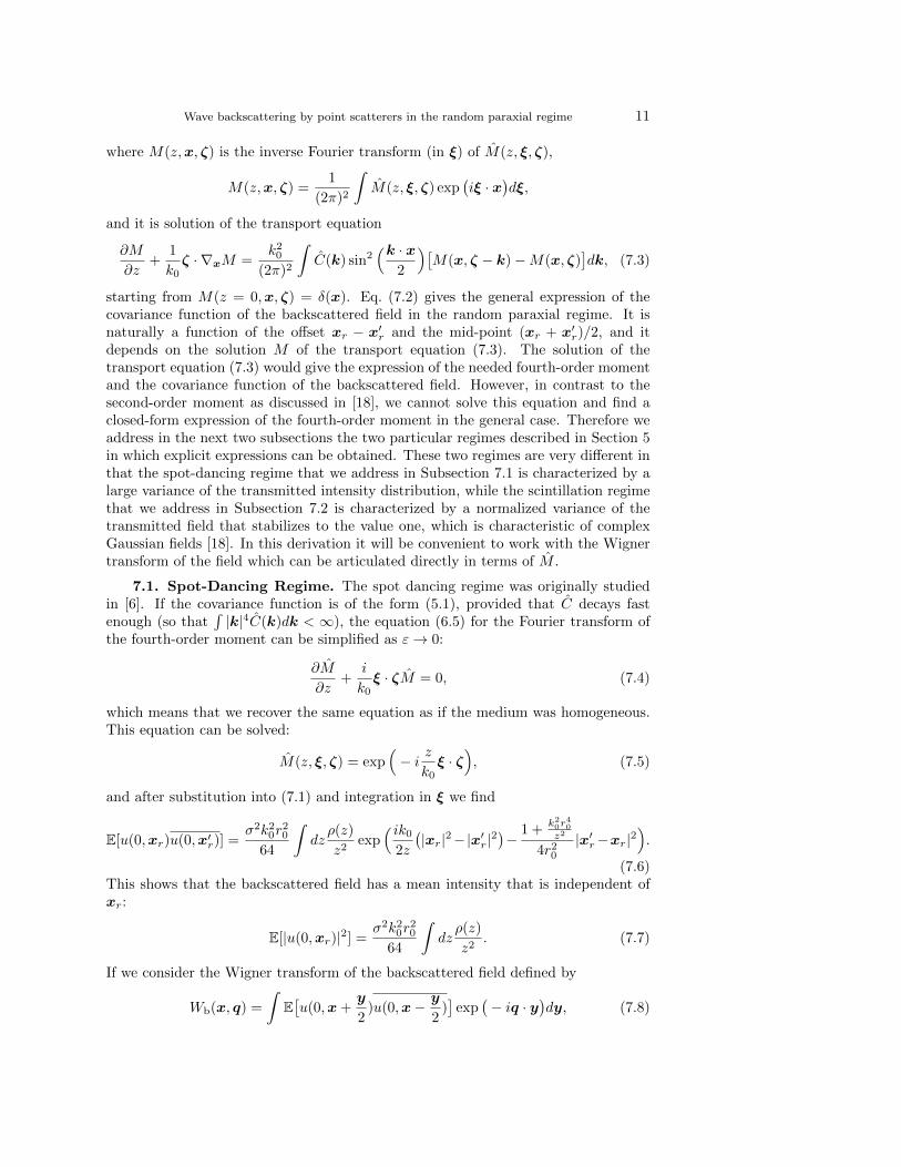
γ = 1.25 10−3 and for lc = 16 we have γ = 3.125 10−4. We use a split-step Fouriermethod for discretizing the paraxial wave propagation. Finally, we perform a series of20000 independent simulations (with independent realizations of the random mediumand of the Poisson cloud of scatterers) to compute the empirical average of the totalenergy flux density I(q) = |u(0, q)|2. Then we compare in Figure 9.1 the empiricalaverage with with the theoretical formula (9.1) for the statistical average, which givesvery good agreement. Note, however, that it is necessary to average over a lot ofrealizations to get the average values.

−0.4 −0.2 0 0.2 0.40.5

1

1.5

2

q

I(q)

−0.4 −0.2 0 0.2 0.40.5

1

1.5

2

q

I(q)

−0.4 −0.2 0 0.2 0.40.5

1

1.5

2

q

I(q)

Fig. 9.1. Mean energy flux density profiles I(q) = |u(0, q)|2 of the backscattered wave. Theblue solid lines are the results of the numerical simulations. The red dashed lines are the theoreticalformulas (9.1). lc = 4 (left), lc = 8 (center), and lc = 16 (right).

10. Conclusion. In this paper we have characterized the multiscale behavior ofthe Wigner distribution of the waves backscattered from a cloud of point scatterersand propagating through a turbulent medium (Proposition 7.2). This has allowed usto describe quantitatively the enhanced backscattering phenomenon. We have shownthat it is possible to estimate the statistical properties of the turbulent medium fromthe wave backscattering in the scintillation regime. This requires to look at the angulardistribution of the received backscattered wave energy flux, and not at the spatialdistribution of the wave intensity. In practice, it is possible to use the time-windowingtechnique in order to select the contributions of the waves backscattered from a givendistance zb from an extended Poisson cloud of point scatterers. By doing so, and byfitting the measured Wigner transform, that is to say, the angular distribution of thereceived wave energy flux, it is possible to estimate both the Hurst parameter H andthe medium parameter γH from the shape of the enhanced backscattering cone. Thiscould be useful for instance to implement efficient deblurring strategies in imagingthrough the atmosphere [23, 28].Note that the Wigner transform or the angular distribution of the backscatteredenergy flux are not statistically stable quantities. This means that it is necessary toaverage over many shots to ensure the statistical stability of the measured quantitiesand allow for their processing for medium parameter estimation.

Acknowledgements. This work was partly supported by AFOSR grant # FA9550-11-1-0176 and by ERC Advanced Grant Project MULTIMOD-267184.

Appendix A. Proof of Proposition 7.1. Here we give a detailed proof ofProposition 7.1. We denote by ‖ · ‖∞ the L∞(R2 × R2)-norm:

‖M‖∞ = supξ,ζ∈R2

|M(ξ, ζ)|.


For any z ≥ 0 we introduce the linear operator Fεz that is bounded from L∞(R2×R2)to L∞(R2 × R2) with a norm smaller than 2k20C(0):

FεzM(ξ, ζ) =k20

4(2π)2

∫C(k)

[2M(ξ − k, ζ)ei

zεk0

k·ζ + 2M(ξ, ζ − k)eiz

εk0k·ξ

−2M(ξ, ζ)−M(ξ − k, ζ − k)eiz

εk0(k·(ξ+ζ)−|k|2)

−M(ξ + k, ζ − k)eiz

εk0(k·(ξ−ζ)+|k|2)

]dk. (A.1)

We denote

Rεz(ξ, ζ) = Mε(z, ξ, ζ)−(M0(z,ξ

ε

)+ M0

(z,ζ

ε

)− exp

(− k20C(0)z

2

)). (A.2)

We need to show that supz∈[0,Z] ‖Rεz‖∞ converges to 0 as ε→ 0. By denoting

Nz(ξ) = M0(z, ξ)− exp(− k20C(0)z

2

), (A.3)

we find that Rεz is solution of

∂Rεz∂z

= Fεz Rεz + Sεz + T εz ,

starting from Rεz=0(ξ, ζ) = 0. Here we have introduced

Sεz(ξ, ζ) =k20

2(2π)2

∫C(k)ei

zεk0

k·ζNz(ξ − k

ε

)dk

+k20

2(2π)2

∫C(k)ei

zεk0

k·ξNz(ζ − k

ε

)dk

− k204(2π)2

∫C(k)ei

zεk0

(k·(ξ+ζ)−|k|2)(Nz(ξ − k

ε

)+ Nz

(ζ − kε

))dk

− k204(2π)2

∫C(k)ei

zεk0

(k·(ξ−ζ)+|k|2)(Nz(ξ + k

ε

)+ Nz

(ζ − kε

))dk,

T εz (ξ, ζ) = − exp(− k20C(0)z

2

) k204(2π)2

∫C(k)

(ei

zεk0

(k·(ξ+ζ)−|k|2)

+eiz

εk0(k·(ξ−ζ)+|k|2)

)dk.

Step 1. For any η > 0,

supz∈[0,η]

‖Rεz‖∞ ≤ 4k20C(0)ηe2k20C(0)η,

uniformly in ε > 0.Since Nz is bounded by 1 in L∞(R2) uniformly in z, Sεz and T εz are bounded by2k20C(0) in L∞(R2 × R2) uniformly in z. Therefore for any z ∈ [0, η] we have

‖Rεz‖∞ ≤ 2k20C(0)

∫ z

0

‖Rεz′‖∞dz′ + 4k20C(0)η


By Gronwall lemma we get the desired result.

Step 2. For any Z > η > 0,

supz∈[0,Z]

‖Rεz‖∞ ≤[4k20C(0)ηe2k

20C(0)η+(Z−η) sup

z∈[η,Z]

(‖Sεz‖∞+‖T εz ‖∞

)]e2k

20C(0)(Z−η),

uniformly in ε > 0.For any z ∈ [η, Z] we have

‖Rεz‖∞ ≤ 2k20C(0)

∫ z

η

‖Rεz′‖∞dz′ + ‖Rεη‖∞ + (Z − η) supz′∈[η,Z]

(‖Sεz′‖∞ + ‖T εz′‖∞

).

By Gronwall lemma we find

supz∈[η,Z]

‖Rεz‖∞ ≤[‖Rεη‖∞ + (Z − η) sup

z∈[η,Z]

(‖Sεz‖∞ + ‖T εz ‖∞

)]e2k

20C(0)(Z−η),

which completes the proof of Step 2 by using Step 1.

Step 3. For any Z > 0, supz∈[0,Z] ‖Sεz‖∞ goes to zero as ε→ 0.It is sufficient to show that, for any Z > 0,

supz∈[0,Z],ξ∈R2

∣∣∣ ∫ C(k)∣∣Nz(ξ − k

ε

)∣∣dk∣∣∣ ε→0−→ 0.

First we remark that∣∣Nz(kε

)∣∣ = exp(− k20C(0)z

2

)∣∣∣ exp(k20

2

∫ z

0

C(z′k

εk0)dz′

)− 1∣∣∣ ≤ k20

2

∫ z

0

|C(z′k

εk0)|dz′,

because ex− 1 ≤ exx for any x ≥ 0 and supx∈R2 |C(x)| ≤ C(0). On the one hand, wehave for any k ∣∣Nz(k

ε

)∣∣ ≤ k202C(0)z,

and on the other hand, for any k 6= 0,∣∣Nz(kε

)∣∣ ≤ εk302|k|

∫ (z|k|)/(εk0)

0

|C(sk

|k|)|ds ≤ εk30

2|k|

∫ ∞0

|C(sk

|k|)|ds,

which shows that, for k ∈ R2 and any z ∈ [0, Z]:∣∣Nz(kε

)∣∣ ≤ K( ε

|k|∧ 1),

where the constant K depends only on Z, k0, C(0), and supe∈S1∫∞0|C(es)|ds. This

gives for any ξ ∈ R2, ε < 1, and any z ∈ [0, Z]:∣∣∣ ∫ C(ξ − k)∣∣Nz(k

ε

)∣∣dk∣∣∣ ≤ K ∫ C(ξ − k)( ε

|k|∧ 1)dk

≤ K[ ∫|k|≤ε1/3

C(ξ − k)dk +

∫|k|>ε1/3

ε

|k|C(ξ − k)dk

]≤ K

[πε2/3 sup

k∈R2

|C(k)|+ ε2/3∫R2

C(ξ − k)dk]

≤ Kε2/3[π supk∈R2

|C(k)|+ (2π)2C(0)],


which completes the proof of Step 3.

Step 4. For any Z > η > 0, supz∈[η,Z] ‖T εz ‖∞ goes to zero as ε→ 0.It is sufficient to show that

supξ∈R2

∣∣∣ ∫ C(k)eiN(k·ξ+|k|2)dk∣∣∣ N→∞−→ 0.

We rewrite ∫C(k)eiN(k·ξ+|k|2)dk =

∫C(k − ξ

2

)eiN |k|

2−iN |ξ|2

4 dk,

By Parseval’s formula, for any q > 0, we have∫C(k)eiN(k·ξ+|k|2)−q2|k|2dk =

π

q2 − iN

∫C(x)e

− |Nξ−x|2

4(q2−iN) dx.

Letting q → 0 (and assuming C, C ∈ L1) gives the generalized Parseval’s formula∫C(k)eiN(k·ξ+|k|2)dk =

iπ

N

∫C(x)ei

ξ2 ·x−i

|x|24N −iN

|ξ|24 dx.

This shows that

supξ∈R2

∣∣∣ ∫ C(k)eiN(k·ξ+|k|2)dk∣∣∣ ≤ π

N

∫|C(x)|dx,

which completes the proof of Step 4.

Step 5. For any Z > 0 we have

limε→0

supz∈[0,Z]

‖Rεz‖∞ = 0.

Combining Steps 2, 3 and 4, we find that, for any Z > η > 0,

lim supε→0

supz∈[0,Z]

‖Rεz‖∞ ≤ 4k20C(0)ηe2k20C(0)η.

Since this holds true for any η > 0, we can let η → 0 to get the desired result.

REFERENCES

[1] L. C. Andrews and R. L. Philipps, Laser Beam Propagation Through Random Media, SPIEPress, Bellingham, 2005.

[2] G. Bal and O. Pinaud, Dynamics of wave scintillation in random media, Comm. Partial Differ-ential Equations 35 (2010), 1176-1235.

[3] Y. N. Barabanenkov, Wave corrections for the transfer equation for backward scattering, Izv.Vyssh. Uchebn. Zaved. Radiofiz. 16 (1973), 88-96.

[4] P. Blomgren, G. Papanicolaou, and H. Zhao, Super-resolution in time-reversal acoustics, J.Acoust. Soc. Am. 111 (2002), 230-248.

[5] J. Chrzanowski, J. Kirkiewicz, and Yu. A. Kravtsov, Influence of enhanced backscatteringphenomenon on laser measurements of dust and aerosols content in a turbulent atmosphere,Phys. Lett. A 300 (2002), 298-302.

[6] D. Dawson and G. Papanicolaou, A random wave process, Appl. Math. Optim. 12 (1984),97-114.


[7] M. V. de Hoop, J. Garnier, and K. Sølna, Enhanced and specular backscattering in randommedia, Waves in Random and Complex Media 22 (2012), 505-530.

[8] A. C. Fannjiang, Self-averaging radiative transfer for parabolic waves, C. R. Acad. Sci. Paris,Ser. I 342 (2006), 109-114.

[9] A. Fannjiang and K. Sølna, Superresolution and duality for time-reversal of waves in randommedia, Phys. Lett. A 352 (2005), 22-29.

[10] R. L. Fante, Electromagnetic beam propagation in turbulent media, Proc. IEEE 63 (1975),1669-1692.

[11] J.-P. Fouque, J. Garnier, G. Papanicolaou, and K. Sølna, Wave Propagation and Time Reversalin Randomly Layered Media, Springer, New York, 2007.

[12] J.-P. Fouque, G. Papanicolaou, and Y. Samuelides, Forward and Markov approximation: thestrong-intensity-fluctuations regime revisited, Waves in Random Media 8 (1998), 303-314.

[13] K. Furutsu, Statistical theory of wave propagation in a random medium and the irradiancedistribution function, J. Opt. Soc. Am. 62 (1972), 240-254.

[14] K. Furutsu and Y. Furuhama, Spot dancing and relative saturation phenomena of irradiancescintillation of optical beams in a random medium, Optica 20 (1973), 707-719.

[15] J. Garnier and K. Sølna, Random backscattering in the parabolic scaling, J. Stat. Phys. 131(2008), 445-486.

[16] J. Garnier and K. Sølna, Coupled paraxial wave equations in random media in the white-noiseregime, Ann. Appl. Probab. 19 (2009), 318-346.

[17] J. Garnier and K. Sølna, Scaling limits for wave pulse transmission and reflection operators,Wave Motion 46 (2009), 122-143.

[18] J. Garnier and K. Sølna, Scintillation in the white-noise paraxial regime, to appear in Comm.Partial Differential Equations.

[19] I. S. Gradshteyn and I. M. Ryzhik, Tables of Integrals, Series, and Products, Academic Press,San Diego, 2007.

[20] A. Ishimaru, Wave Propagation and Scattering in Random Media, Academic Press, San Diego,1978.

[21] J. F. C. Kingman, Poisson Processes, Clarendon Press, Oxford, 1993.[22] G. Labeyrie, F. de Tomasi, J.-C. Bernard, C. A. Muller, C. Miniatura, and R. Kaiser, Coherent

backscattering of light by atoms, Phys. Rev. Lett. 83 (1999), 5266-5269.[23] Y. Mao and J. Gilles, Non rigid geometric distortions correction - Application to atmospheric

turbulence stabilization, Inverse Problems and Imaging 6 (2012), 531-546.[24] Y. Miyahara, Stochastic evolution equations and white noise analysis, Carleton Mathematical

Lecture Notes 42, Ottawa, Canada, (1982), 1-80.[25] G. Papanicolaou, L. Ryzhik, and K. Sølna, Self-averaging from lateral diversity in the Ito-

Schrodinger equation, SIAM Multiscale Model. Simul. 6 (2007), 468-492.[26] J. W. Strohbehn, ed., Laser Beam Propagation in the Atmosphere, Springer, Berlin, 1978.[27] V. I. Tatarskii, A. Ishimaru, and V. U. Zavorotny, eds., Wave Propagation in Random Media

(Scintillation), SPIE Press, Bellingham, 1993.[28] D. H. Tofsted, Reanalysis of turbulence effects on short-exposure passive imaging, Opt. Eng.

50 (2011), 016001.[29] A. Tourin, A. Derode, P. Roux, B. A. van Tiggelen, and M. Fink, Time-dependent coherent

backscattering of acoustic waves, Phys. Rev. Lett. 79 (1997), 3637-3639.[30] B. J. Ucsinski, Analytical solution of the fourth-moment equation and interpretation as a set

of phase screens, J. Opt. Soc. Am. A 2 (1985), 2077-2091.[31] G. C. Valley and D. L. Knepp, Application of joint Gaussian statistics to interplanetary scin-

tillation, J. Geophys. Res. 81 (1976), 4723-4730.[32] M. P. van Albada and A. Lagendijk, Observation of weak localization of light in a random

medium, Phys. Rev. Lett. 55 (1985), 2692-2695.[33] M. C. W. van Rossum and Th. M. Nieuwenhuizen, Multiple scattering of classical waves:

Microscopy, mesoscopy, and diffusion. Rev. Modern. Phys. 71 (1999), 313-371.[34] A. M. Whitman and M. J. Beran, Two-scale solution for atmospheric scintillation, J. Opt. Soc.

Am. A 2 (1985), 2133-2143.[35] P. E. Wolf and G. Maret, Weak localization and coherent backscattering of photons in disor-

dered media, Phys. Rev. Lett. 55 (1985), 2696-2699.[36] I. G. Yakushkin, Moments of field propagating in randomly inhomogeneous medium in the limit

of saturated fluctuations, Radiophys. Quantum Electron. 21 (1978), 835-840.

Documents

WAVE BACKSCATTERING BY POINT …ksolna/research/92scatt.pdfwave backscattering by point scatterers in the random paraxial regime josselin garnier and knut s˜lnay and knut s˜lnayPublished