Wave and Tidal Energy Yield Uncertainty - ORE Catapult · 2018-01-23 · Tidal energy is essentially deterministic (driven by the position of the sun and moon relative to the earth),

Wave and Tidal Energy Yield Uncertainty

Reference Document

July 2015

Wave and Tidal Energy Yield Uncertainty PN000083-SRT-005

ORE Catapult 1

Document History

Disclaimer: The information contained in this report is for general information and is provided by

Frazer-Nash Consultancy. Whilst we endeavour to keep the information up to date and correct,

neither ORE Catapult nor Frazer-Nash Consultancy make any representations or warranties of

any kind, express, or implied about the completeness, accuracy or reliability of the information

and related graphics. Any reliance you place on this information is at your own risk and in no

event shall ORE Catapult or Frazer-Nash Consultancy be held liable for any loss, damage

including without limitation indirect or consequential damage or any loss or damage whatsoever

arising from reliance on same.

Field Detail

Report Title Wave and Tidal Energy Yield Uncertainty

Report Sub-Title Reference Document

Client/Funding CORE

Status Public

Project Reference PN000083

Document Reference PN000083-SRT-005

Revision Date Prepared

by

Checked

by

Approved

by

Revision History

1 April 2015 Stephen

Livermore

Neil

Adams

Brian

Gribben None


ORE Catapult 2

Frazer-Nash Consultancy provides independent technical advice to customers across a wide

range of industries. In marine renewables, they support device developers, project developers

and investors to design more effective systems, mitigate risk and reduce costs. Their track-

record in this field includes resource assessment, array layout optimisation and energy yield

uncertainty estimation on several of the leading marine energy projects.

www.fnc.co.uk


ORE Catapult 3

Contents

1 Introduction............................................................................................................. 4

2 Uncertainty Assessment ........................................................................................ 5

2.1 Background ...................................................................................................... 5

2.2 Sources of Uncertainty ..................................................................................... 6

2.3 Combining Individual Uncertainties .................................................................. 7

3 Energy Yield Prediction ......................................................................................... 8

3.1 Tidal Energy ..................................................................................................... 8

3.2 Wave Energy ................................................................................................. 11

4 Reference Projects ............................................................................................... 14

4.1 Tidal Energy Turbines .................................................................................... 14

4.2 Wave Energy Convertor: Attenuator-Type ..................................................... 16

4.3 Wave Energy Convertor: Oscillating Wave Surge .......................................... 17

5 Uncertainty Assessment Guidance .................................................................... 19

5.1 Discussion ..................................................................................................... 20

6 Conclusions .......................................................................................................... 33

7 References ............................................................................................................ 34

8 Acknowledgements .............................................................................................. 35

Annex A ....................................................................................................................... 36


ORE Catapult 4

1 Introduction

The Marine Farm Accelerator (MFA) has the aim of quantifying and reducing the uncertainties

associated with energy yield predictions of marine energy projects. The process of determining

uncertainty predictions on energy yield is reasonably well developed in the wind industry but is

relatively immature in the wave and tidal energy sectors. As these industries develop, potential

investors will need to know not only the most likely revenue that the project may deliver but also

the uncertainty on that revenue. Consequently, there is a requirement to assess methods of

quantifying uncertainty and to standardise the process of reporting uncertainty within the wave

and tidal energy industries.

The MFA has taken an important first step in this process with the development of a Taxonomy

Document which lists the losses and uncertainties that should be considered as part of an

Energy Production Estimate (EPE). This current Reference Document has been developed to

provide guidance for determining the uncertainties highlighted in this taxonomy document. It is

the result of an industry-wide research study involving two main components:

Literature Review of relevant industry standards, technical guides as well as academic

papers, conference proceedings and books;

Stakeholder Engagement involving interviews with industry practitioners including

consultants, device and project developers, surveyors and modellers, and academics.

Together these two activities have provided a consolidated view of the state-of-the-art of

uncertainty assessment within the wave and tidal energy sectors and this information has been

used to provide best practice guidance on the assessment of the individual uncertainty

categories and how they should be combined to inform an overall project uncertainty.

This guidance has been applied to a series of example projects to demonstrate the variation in

approaches that can be undertaken. Much of this variation arises from the process by which

the EPE is calculated in the first place. This document provides a summary of the different

approaches for determining the EPE and the uncertainties which are relevant to these

approaches. Although the wave and tidal uncertainty categories in the taxonomy document are

the same, the ways in which they should be addressed and the current levels of understanding

differ significantly. Tidal energy is essentially deterministic (driven by the position of the sun

and moon relative to the earth), whilst wave energy is stochastic (driven by the weather). The

tidal energy industry is also more mature and this is reflected in the greater variety of modelling

options available. As a result, wave and tidal energy are largely considered separately in this

document.

The final aspect of this project has been the development of an Interactive Uncertainty Tool

which provides a standardised method for the uncertainty assessment. This tool has been

applied to the example projects to record and present the results.


ORE Catapult 5

2 Uncertainty Assessment

2.1 Background

Any energy yield prediction is subject to some uncertainty. Even the most thorough resource

assessment campaign will give an imperfect knowledge of the resource at the site. This

uncertainty grows when trying to extrapolate the outputs of that resource assessment exercise

in space or time, and is compounded again by the uncertainties in plant performance.

When taking measurements and undertaking modelling, usually a single estimate of energy

yield will be obtained. At best, this estimate has a 50% chance of being too high, and a 50%

chance of being too low. The purpose of an uncertainty assessment is to work out how far out

the model predictions are likely to be from the real energy yield. In this context energy yield

uncertainty is the degree of precision with which an energy yield is predicted.

Uncertainties are particularly important to financiers since energy yield uncertainty translates

directly into uncertainty on the revenue that a project will generate. Consider a project funded by

debt finance. If the project revenues are roughly as expected, the loans are serviced and the

owners make a modest return. If the project does better than expected, the owners of the

project reap the benefit, but the debt providers do not see any additional return. However, if the

project does not do as well as expected, the development company may be unable to service its

debt and the debt providers will lose out. Debt providers are therefore much more exposed to

the downside risks of uncertainty than the upside benefits.

Investors need to understand energy yield uncertainty to gauge the risks associated with their

investments. A process for assessing uncertainties has become fairly well-developed in the

wind industry. This involves working through a “taxonomy” of potential sources of uncertainty,

and assigning a value to each one. These uncertainties are usually then combined using a root-

sum-squares method to determine an overall energy yield uncertainty for the project. Finally,

this uncertainty is used to calculate energy yields that have specific exceedance probabilities –

for example, the central estimate from the modelling is termed the P50, and it has a 50%

chance of being exceeded.

Finance arrangements vary from project to project but for debt finance to wind energy projects

in the UK, it is typical that the investor will determine the maximum loan size they are willing to

extend based on the P90; that is, the energy yield that has a 90% chance of being exceeded.

An investor will size the loan such that the annual revenue at the P90 level is a certain factor

greater than the interest payments on the loan. This factor is known as the Debt Service

Coverage Ratio (DSCR) and a DSCR of 1.4 based on the P90 is typical for onshore wind

projects in the UK, whereas some American investors use a DSCR of 1 based on the P99 (i.e.

the energy yield that has a 99% chance of being exceeded). The lower the uncertainty on the

project, the closer the P90 and P99 are to the P50, so the greater the proportion of the


ORE Catapult 6

development cost that can be covered by debt finance. This means that equity investors can put

in a smaller investment and achieve a greater return on that investment.

Figure 1: Example Energy Yield Uncertainty Assessment

Figure 1 illustrates an example energy yield uncertainty assessment derived from the Interactive

Uncertainty Tool developed as part of this project. The average (median) energy yield is

15GWh/yr and there is an overall uncertainty of 20% on this yield. The normalised probability

density is shown by the red line and the exceedance probability by the blue line. In this

example, the P90 energy yield is 11.2 GWh/yr and the P99 yield is 8.0 GWh/yr.

This of course relies on the assumption that the P50 and the uncertainty can be estimated

reliably. One of the key aims of this reference document is to standardise the approach for

calculating uncertainty.

2.2 Sources of Uncertainty

Following the approach used in the wind industry, the uncertainty in energy yield for tidal and

wave projects is determined as follows:

All of the uncertainties which affect the resource at the project site are identified and

grouped together. Principally this includes uncertainties associated with site

measurements and modelling of the resource. For tidal, the uncertainties are quantified in

current speed and for wave these are height and wave period separately. These

uncertainties are then summed in quadrature.


ORE Catapult 7

A sensitivity study is used to quantify how sensitive the energy yield is to the available

resource. For example, for tidal this provides a mapping from current speed to available

power of the resource and this is used to convert that resource uncertainty into an energy

yield uncertainty (in MWh/yr);

This is combined with all of the other energy uncertainties (i.e. all other factors quantified

in MWh/yr, e.g. device power performance, availability, device interactions and electrical

losses) and summed in quadrature to derive the overall energy uncertainty.

2.3 Combining Individual Uncertainties

Typically in wind energy uncertainty assessments, the overall uncertainty is derived by

combining individual uncertainties using a root-sum-squares (RSS) approach. This assumes

that the individual errors are uncorrelated and can be approximated as normal distributions. It

also relies on a mathematical approximation - that the central limit theorem is applicable to

multiplication of uncertain variables as well as addition – which in any case is only valid for

small uncertainty levels.

The wind industry has become comfortable with these assumptions and approximations.

However, for wave and tidal, there are reasons to believe that they may no longer be valid. For

example, if the overall uncertainty is dominated by one or two contributors which are not

normally distributed, the end result will not be normally distributed. If the overall uncertainty is

higher than in wind, the validity of the central limit theorem may reduce.

In principle, Monte-Carlo simulation has the potential to overcome these problems. However,

this is more complex and time-consuming than the root-sum-squares method and the results

are less intuitive to interpret. While these considerations should be kept in mind, based on

experience and knowledge of statistical analysis including Monte-Carlo simulations, it is

considered that an RSS approach remains appropriate for typical marine energy applications

where the P90:P50 ratio is the main focus. For this reason the Interactive Uncertainty Tool has

been configured to use the RSS approach.


ORE Catapult 8

3 Energy Yield Prediction

There are many potential approaches to estimating the energy yield for a tidal or wave energy

project depending on the number of devices proposed, the level of accuracy required and the

spatial variation of the resource across the site. Consequently, the way in which uncertainties

are evaluated depends on the approach to the energy yield calculation. The purpose of this

section is to explain these different methods and provide context for the uncertainty assessment

developed in Section 5. The methods described here are generally consistent with the IEC

Technical Specifications (References 1 to 4) and any deviations are highlighted.

3.1 Tidal Energy

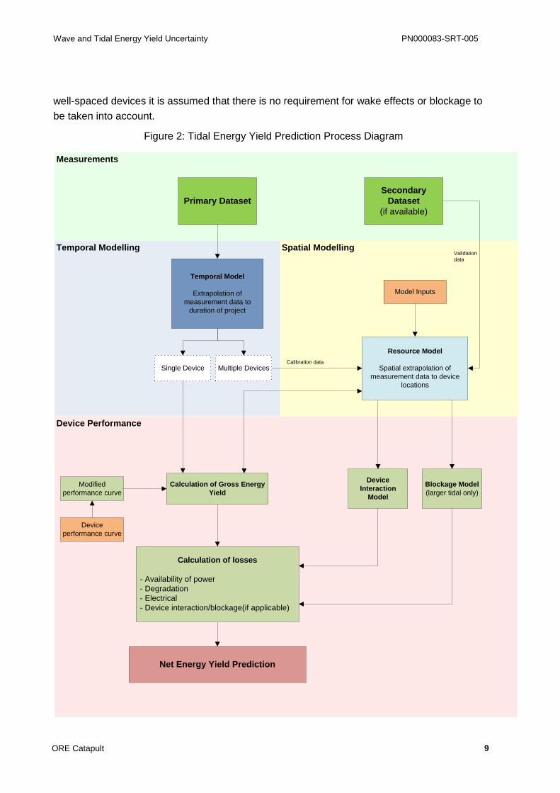
Figure 2 illustrates a typical process for determining the net energy yield for a tidal site. Where

there are measurement data at all of the proposed device locations it is not necessary to

undertake resource modelling and a simplified approach involving temporal modelling only is

appropriate (Method 1, Section 3.1.1). For larger sites, or any small development where

resource measurements have not been made at each device location, resource modelling is

needed in addition to the temporal modelling and Method 2 is generally appropriate (Section

3.1.2). This is consistent with the IEC Technical Specifications (References 1 and 2).

3.1.1 Method 1: Single Device - Temporal Modelling

Long-term predictions of tidal currents for resource assessments are generally provided by

models which are calibrated using a time series of tidal current measurement data. Tidal

currents are deterministic, although they may be affected to a lesser or greater extent by

stochastic meteorological events (waves and storm surge) and turbulence. Harmonic analysis

is undertaken on measurements from the location of the proposed device to extract the principle

constituents. These constituents are modified to take into account the variability of longer-term

astronomical effects and are then extrapolated to determine the current speed and direction at

the turbine location for the proposed duration of the project. Since measurements are taken at

the device location, no spatial modelling is required.

The projected tidal or wave resources are then combined with the tidal device performance

curve to determine the gross energy yield. This is assumed to have been measured in

accordance with IEC Technical Specification (Reference 2) at a facility such as EMEC. If

necessary, this may be modified to account for differences between the conditions at the test

site and the project site. Such modifications are not specified in the IEC Technical Specification

but this is emerging as best practice in the wind industry. Efforts are ongoing to develop and

validate methods for this in the tidal energy sector (e.g. TIME project).

Finally, energy losses resulting from availability, degradation and electrical transmission are

calculated to determine the net energy yield prediction. For either a single or limited number of


ORE Catapult 9

well-spaced devices it is assumed that there is no requirement for wake effects or blockage to

be taken into account.

Figure 2: Tidal Energy Yield Prediction Process Diagram

Device Performance

Spatial ModellingTemporal Modelling

Measurements

Primary Dataset

Secondary

Dataset

(if available)

Temporal Model

Extrapolation of

measurement data to

duration of project

Single Device Multiple Devices

Resource Model

Spatial extrapolation of

measurement data to device

locations

Model Inputs

Calculation of Gross Energy

Yield

Device

Interaction

Model

Device

performance curve

Modified

performance curve

Blockage Model

(larger tidal only)

Calculation of losses

- Availability of power

- Degradation

- Electrical

- Device interaction/blockage(if applicable)

Net Energy Yield Prediction

Validation

data

Calibration data


ORE Catapult 10

3.1.2 Method 2: Multiple Devices – Temporal and Spatial Modelling

For projects with more than one device, it is generally not feasible to undertake measurement

campaigns at all proposed device locations and spatial modelling must be undertaken to predict

the variation in tidal resource across the site. This is generally undertaken using a 2D depth-

averaged modelling code such as Mike21, Telemac or Delft3D. The inputs to the model are

boundary conditions (e.g. tidal elevations at a considerable distance away from the area of

interest, such as the continental shelf), bathymetry, bed roughness and potentially

meteorological data for capturing the wave climate. Measurement data from a location near to

the turbines (primary dataset) is used to calibrate the model. If additional datasets are available

(secondary datasets in Figure 2), these can be used to validate the model and hence quantify

its uncertainty. A more refined and/or sophisticated model may also be used, e.g. 3D CFD, to

capture local effects. Usually such a model will be driven with boundary conditions derived from

a larger-scale 2D model.

The gross energy yield is determined in the same manner as a single device, by combining with

the device performance curve. The net energy yield is then calculated by deducting the various

losses. For sites where there are multiple devices, wake interactions and potentially blockage

become important. Ideally, the spatial variation of resource, wake losses and blockage would

be captured in a single model. In practice, this is challenging as no single model configured for

practical computational effort captures all of these scales well. For example:

2D depth-averaged models (e.g. Mike21) solve the shallow water equations by finite

volume or finite element methods. These can predict spatial variations of a resource but

provide no detail on the vertical profile of the flow. These allow feedback effects such as

blockage to be modelled, but are unable to capture wake interactions or wake dissipation

accurately.

3D CFD solves the Reynolds-Averaged Navier Stokes (RANS) equations using a finite

volume method. This can be used to model the vertical profile in the resource and also

wake effects, but they are not configured to capture blockage.

Wake models based on engineering tools from the wind industry (e.g. the Ainslie wake

model used in TidalFarmer) can be used to model wake effects but need to be combined

with other flow models to capture the resource and blockage.

Capturing all of these effects requires combining or coupling different models together and the

accuracy of the final result depends on the way models are combined as well as the accuracy of

the individual models.


ORE Catapult 11

3.2 Wave Energy

Figure 3 illustrates the equivalent process for determining the net energy yield for a wave site

and the following subsections explore these processes for single device and multiple device

projects.

3.2.1 Method 1: Single Device – Temporal Modelling

Wave climate is stochastic and measurement data is needed to characterise the long-term

resource variability using either:

Long-term runs of a validated wave model; or the

Measure-Correlate-Predict (MCP) approach as used in the wind industry.

In the first method, a resource model (e.g. SWAN) is used to model the wave climate for the

device location using a period of local hindcast data as input boundary conditions and the

measurement data for validation. For the MCP method, the measurement data is correlated to

some long-term reference data and this correlation is then used to map the long-term local

dataset to the location of the device. The result of both methods is the historical prediction of

the wave climate for the device location.

There is significant evidence that inter-annual variability of wave climates consists of stochastic

and climatic effects. For the UK, this is the correlation of the wave climate with the North

Atlantic Oscillation (NAO). The stochastic effects can be extracted and applied directly and

combined with a probabilistic model of future NAO predictions to model the future climatic

effects. These are combined and aggregated up to the period of the EPE to determine the

projected wave resource for the project.

The projected wave resources are then combined with the wave power matrix to determine the

gross energy yield. As with tidal energy, this is assumed to have been measured in accordance

with the IEC Technical Specification (Reference 4). If necessary this may then be modified to

account for differences between the conditions at the test site and the project site. For either a

single or small number of well-spaced devices, it may be assumed that there is no requirement

for device interaction effects to be taken into account.

3.2.2 Method 2: Multiple Devices – Temporal and Spatial Modelling

The IEC Technical Specification (Reference 3) states that the MCP approach should only be

used for assessment at discrete points and is therefore only considered appropriate for single

device sites. Consequently, only the long-term runs approach is suitable for multiple devices.

The resource model used to predict the historic wave climate is extended to predict the wave

climate at the proposed device locations. This is generally undertaken using third generation

models (e.g. SWAN) as these capture the principal physical effects. If additional measurement

datasets are available these can be used to validate the model.


ORE Catapult 12

Figure 3: Wave Energy Yield Prediction Process Diagram

Temporal &

Spatial Modelling

Measurements

Primary

Databaset

Resource Model

Spatial extrapolation of

measurement data to device

locations

Model InputsCorrelate

Measurement and

Reference Data

Validation

data

Hindcast Data

Long-term

Reference Data

Historical

Prediction

Device

Performance

Gross Yield Predictions

Device Power

Matrix

Modified Power

Matrix

Calculation of losses

- Availability of power

- Degradation

- Electrical

- Device interaction/blockage (if applicable)

Net Energy Yield Prediction

Statistical Analysis

Statistic VariabilityInter-annual Variability

(e.g. NAO)

NAO Future

Predictions

MCP

Historical Prediction

with inter-annual variability

Secondary

Dataset

(if available)

Long-term runs

Device

Interaction

Model


ORE Catapult 13

The gross and net energy yields are then determined by combining with the power matrix.

Various modelling methods can be used to assess device interaction effects, although validation

of these models is currently limited to scale tests so it is difficult to assess their uncertainty.


ORE Catapult 14

4 Reference Projects

This section describes a series of example projects which will be used in Section 5 to

demonstrate the variation in methods of assessing uncertainty. Many of these variations arise

from the different approaches to calculate the EPE (see Section 3) and the purpose of these

projects is to illustrate this through a series of realistic scenarios.

4.1 Tidal Energy Turbines

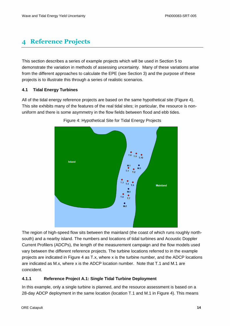
All of the tidal energy reference projects are based on the same hypothetical site (Figure 4).

This site exhibits many of the features of the real tidal sites; in particular, the resource is non-

uniform and there is some asymmetry in the flow fields between flood and ebb tides.

Figure 4: Hypothetical Site for Tidal Energy Projects

The region of high-speed flow sits between the mainland (the coast of which runs roughly north-

south) and a nearby island. The numbers and locations of tidal turbines and Acoustic Doppler

Current Profilers (ADCPs), the length of the measurement campaign and the flow models used

vary between the different reference projects. The turbine locations referred to in the example

projects are indicated in Figure 4 as T.x, where x is the turbine number, and the ADCP locations

are indicated as M.x, where x is the ADCP location number. Note that T.1 and M.1 are

coincident.

4.1.1 Reference Project A.1: Single Tidal Turbine Deployment

In this example, only a single turbine is planned, and the resource assessment is based on a

28-day ADCP deployment in the same location (location T.1 and M.1 in Figure 4). This means


ORE Catapult 15

that many of the most complex aspects of a “normal” EPE are excluded, i.e. the spatial resource

modelling aspects and the wake effects. Furthermore, turbine availability and power

performance uncertainties are assumed to be completely mitigated by the turbine supply

contract rather than included in the EPE, so these uncertainties are also zero.

However, some uncertainties in the energy yield still remain, and the purpose of this example

project is to explore these. These uncertainties also underpin the later, more complex reference

projects (A.2 to A.5).

4.1.2 Reference Project A.2: 5-Turbine Array, Minimal Data

Reference Projects A.2, A.3 and A.4 all refer to 5-turbine arrays with the same layout (turbines

T.1 to T.5 in Figure 4).

For Project A.2, the EPE is being prepared using a minimal dataset. The only on-site resource

measurements are from a 28-day ADCP deployment at location M.1, and the only flow

modelling is a 2D depth-averaged model (e.g. Mike21).

The turbine power curve is assumed to have been validated in a test deployment (e.g. EMEC)

in accordance with IEC Technical Specification (Reference 2). Power performance and

availability uncertainty are to be included in the EPE, although minimum performance and

availability levels are warranted in the turbine supply contract.

The turbines are laid out so that as far as possible the wakes from the front turbines pass

between the rear turbines but no wake modelling is being performed.

4.1.3 Reference Project A.3: 5-Turbine Array, Moderate Data

This project is as per Reference Project A.2, but with 3D CFD used to model the resource and

wake interactions, with boundary conditions supplied from the Mike21 model. All other

assumptions are as before.

4.1.4 Reference Project A.4: 5-Turbines Array, Maximum Data

This project is as per Reference Project A.3, but with additional measured data to quantify the

variability of the resource and validate the CFD. The ADCP deployment at location M.1 is

extended to 90 days. In parallel, 30-day deployments are undertaken at M.2, M.3 and M.4.

4.1.5 Reference Project A.5: 10-Turbine Array

This project is as per Reference Project A.4, but with turbine locations T.6 to T.10 included in

the array. This project is now anticipated to be above 10MW and according to the IEC

Technical Specification (Reference 1). This means that blockage effects may be significant. In

addition, the outside turbines are further from the ADCP measurement locations which

increases the dependence on the flow model.


ORE Catapult 16

4.2 Wave Energy Convertor: Attenuator-Type

All of the attenuator-type wave energy reference projects are based on the same hypothetical

site, which is shown in Figure 5. This site is at least 5km offshore, so there are no near-shore

effects, although there is a variation in water depth across the site.

All of the wave energy convertors (WECs) are assumed to be Pelamis-like attenuators. Their

power matrix is obtained from numerical modelling validated against sea trials data. The WEC

locations are indicated in Figure 5 as P.x, where x is the device number. The device locations

have water depths between 50m and 70m. Waverider buoy locations are indicated as W.x,

where x is the buoy location number. The spacing between adjacent devices is around 500m.

Figure 5: Hypothetical Site for Attenuator-Type Wave Energy Projects

4.2.1 Reference Project B.1: Single Device Array, Minimal Data

This project consists of one device in location P.1 in Figure 5. The wave climate is derived

based on a 12-month Waverider buoy deployment at the same location (W.1), which is

correlated against 20 years’ hindcast data as a long-term reference using the Measure-

Correlate-Predict (MCP) method. Since there is only one device, resource modelling and

device interaction effects are excluded. Furthermore, the device availability and power

performance uncertainties are assumed to be managed via the device supply contract rather

than included in the EPE, so these uncertainties are zero. However, as with tidal Project A.1

some uncertainties remain, and the purpose of this example is to explore these.

4.2.2 Reference Project B.2: Five-Device Array, More Data

This project consists of 5 WECs in locations P.1. to P.5 in Figure 5. There is more data on the

wave resource with concurrent 12-month deployments of Waverider buoys undertaken at

locations W.1 and W.2. The historical resource is characterised using the long-term runs


ORE Catapult 17

method and the variation of the wave climate across the site is modelled using SWAN.

Interactions between the devices are modelled using potential flow theory.

Power performance and availability uncertainty are to be included in the EPE.

4.2.3 Reference Project B.3: Ten-Device Array

This project is identical to Reference Project B.2, but with ten devices rather than five. The

additional devices are installed in locations P.6 to P.10. The greater number of devices means

that interaction effects and the spatial variation of the resource are more significant in the EPE.

4.3 Wave Energy Convertor: Oscillating Wave Surge

All of the surge-type wave energy reference projects are based on the same hypothetical site,

which is shown in Figure 6. The wave energy convertors (WECs) are assumed to be Oyster-

like nearshore oscillating wave surge convertors.

Their power matrix is obtained from numerical modelling validated against sea trials data. The

WEC locations are indicated in Figure 6 as O.x, where x is the device number. All of the WECs

are in 10m to 15m water depth, between 500m and 1000m from shore. Due to the proximity to

shore, AWACs are used instead of Waverider buoys as they are less susceptible to breaking

waves. The AWAC locations are indicated as W.x, where x is the buoy location number.

Figure 6: Hypothetical Site for Surge-Type Wave Energy Projects

4.3.1 Reference Project C.1: Single Device Array, Minimal Data

This project consists of one device in location O.1 in Figure 6. The wave climate is derived

based on a 12-month AWAC deployment at the same location (W.1), which is correlated against


ORE Catapult 18

20 years’ hindcast data as a long-term reference using the Measure-Correlate-Predict (MCP)

method. Similar to Project B.1, resource modelling and device interaction effects are excluded.

Furthermore, the device availability and power performance uncertainties are assumed to be

managed via the device supply contract rather than included in the EPE, so these uncertainties

are zero.

4.3.2 Reference Project C.2: Five-Device Array, More Data

This project consists of five devices in locations O.1 to O.5 in Figure 6. Concurrent 12-month

deployments of AWACs are undertaken at locations W.1 and W.2, and the variation of the wave

climate across the site is modelled using SWAN. This model is run for 20 years to evaluate the

long-term resource. Interactions between devices are included in the SWAN model, but are

shown to be negligible.

Power performance and availability uncertainty are to be included in the EPE.

4.3.3 Reference Project C.3: Ten-Device Array

This project is identical to Reference Project C.2, but with ten devices rather than five. The

additional devices are installed in locations O.6 to O.10. The greater number of devices means

that the spatial variation of the resource is more significant in the EPE, although SWAN

modelling confirms that interaction effects are still negligible.


ORE Catapult 19

5 Uncertainty Assessment Guidance

This section provides guidance on how the various individual uncertainties given in the

Taxonomy Document may be assessed. Whilst the wave and tidal taxonomy categories are the

same, the manner in which they are addressed is different in some cases and consequently

they are considered separately in Table 4 (tidal) and Table 5 (wave). For each uncertainty

category a description is provided of how the uncertainty arises and how it can be determined.

The intention is to provide generalised guidance which can be used to construct uncertainty

assessments for future projects.

This information is then applied to the example projects described in Section 4 and the

individual uncertainties relevant to these projects are shown in separate columns within the

tables. The wave example projects (attenuator-type (Project B) and oscillating surge wave

convertors (Project C)) are both combined within Table 5 but any differences between these

types of devices are stated.

All projects are hypothetical examples and no modelling has been undertaken to quantify the

specific uncertainties. The values given for the uncertainties are either known (e.g. provided by

equipment manufacturer), calculated based on information provided, extracted from relevant

sources or in some cases estimated based on judgment of appropriate values. In particular, the

uncertainties associated with the spatial modelling for both tidal and wave are highly site

specific and as such these values have generally been estimated.

The first three uncertainty categories (Measurement, Temporal Extrapolation and Spatial

Extrapolation) are based on resource parameters (mean current speed for tidal and significant

wave height and energy period for wave), rather than energy yield. These uncertainties are

converted to energy by a sensitivity study; essentially perturbing the resource parameter and

studying the effect on the energy yield. For tidal, this is by perturbing the velocity magnitudes in

the resource model and for wave this is the wave height and energy period. In both cases it is

typical to use a perturbation of +/-5%, although best practice would be to test a range of values

to check for any strong non-linearity. These converted uncertainties are then combined with

those associated with the device performance to give the uncertainty in energy yield. For all

example projects considered here the following sensitivity factors have been applied. These

are considered to be realistic but by no means universally applicable.

Tidal - Sensitivity of energy yield to mean flow speed (1.7);

Wave - Sensitivity of energy yield to significant wave height (1.3) and energy period (0.8).

All uncertainties are given as percentages, and are normalised on the average power or

resource parameters as appropriate. The individual uncertainties have been combined using

the Interactive Uncertainty Tool and an illustration of this is shown in Annex A. This is a

structured worksheet which allows users to consolidate all the individual uncertainties with


ORE Catapult 20

comments and supporting evidence. The tool then combines the uncertainties, applying the

sensitivity factor where applicable, and outputs the overall uncertainty, along with the key

exceedance values: P50, P75, P90, P95 and P99. The tool also illustrates the probability

distribution and the relative magnitude of the different uncertainty sub-categories. In wave,

uncertainties for significant wave height and energy period are generally assumed to be

uncorrelated but the tool allows for a correlation coefficient to be applied if appropriate. The

true degree of correlation depends on the origin of the uncertainty.

5.1 Discussion

The overall project uncertainties for the tidal and wave reference projects are presented in

Table 1 to Table 3. These reference projects have highlighted some important themes which

are summarised as follows:

The values of the uncertainties will vary from site to site, but the results achieved here

demonstrate the expected trend, i.e. that investments in additional modelling and

measurement activities can deliver reductions in uncertainty. This approach should be

useful for project developers to help them decide how to target the available budget to

achieve maximum reductions in uncertainty.

Measurement uncertainties inherent to the instruments themselves are reasonably small

and well-understood in both wave and tidal. There are various ways in which these

uncertainties can grow when deployed in non-ideal conditions although these can be

avoided by good practice and quality control procedures.

Temporal extrapolation procedures are fundamentally different in wave and tidal projects:

tidal flows are largely deterministic (driven by the positions of the sun and moon relative to

the earth) whereas waves are stochastic (driven by the weather). In tidal, the uncertainty

associated with harmonic analysis is low but the key challenges are dealing with sites with

substantially asymmetric flow regimes and accounting for non-astronomical effects. In

particular, wave-current interaction is not well understood, so sites where currents are

strongly affected by non-meteorological effects will have increased uncertainty. For the

reference projects it was assumed that the locations were sheltered so this effect is

negligible. In wave, the inter-annual variability appears to be strongly site-specific.

Methods to capture this are well known from the wind industry, although there is evidence

that wave climates are correlated to climatic indices such as the North Atlantic Oscillation

(NAO), as these affect storm tracks. Methods of quantifying and accounting for this

sensitivity are available in the literature and are used here.

Spatial extrapolation is a key area of uncertainty in both wave and tidal, and becomes

increasingly important for larger sites. Higher-fidelity modelling (e.g. 3D CFD) can be

used to reduce the uncertainty in tidal energy, but this reduced uncertainty needs to be

demonstrated via sensitivity studies or on-site validation rather than being assumed

because of the choice of models used.


ORE Catapult 21

Power performance and performance degradation are potentially significant sources of

uncertainty. There are site-specific effects which can affect the performance of the

devices, e.g. the turbulence levels in tidal flows and the spectral shape of wave fields.

Guidance on assessing the uncertainties in power performance tests is available from the

wind industry and is considered to be applicable here.

Device interactions constitute a significant uncertainty for larger sites. Various modelling

approaches can be used to predict these effects, but there is a general lack of full-scale

validation.

Availability represents a very significant uncertainty for early wave and tidal energy

projects. This has largely been mitigated in these example projects through contracts with

the device supplier but the extent to which this is achievable in practice will be dependent

on the individual project. It is envisaged that the calculation of uncertainty will improve as

more demonstration and commercial projects are deployed.

Table 1: Uncertainties for Example Tidal Turbine Projects.

Reference Project No. Overall Uncertainty

(%)

A.1 Single tidal turbine 4.0

A.2 5-turbine array, minimal data 20.7

A.3 5-turbine array, moderate data 18.7

A.4 5-turbine array, maximum data 9.4

A.5 10-turbine array 9.7

Table 2: Uncertainties for Example Attenuator-Type Wave Projects.

Reference Project No. Overall Uncertainty (%)

B.1 Single device 4.4

B.2 5-device array 19.2

B.3 10-device array 19.4

Table 3: Uncertainties for Example Oscillating Wave Surge Converter Projects.

Reference Project No. Overall Uncertainty (%)

C.1 Single device 4.5

C.2 5-device array 26.2

C.3 10-device array 26.2


ORE Catapult 22

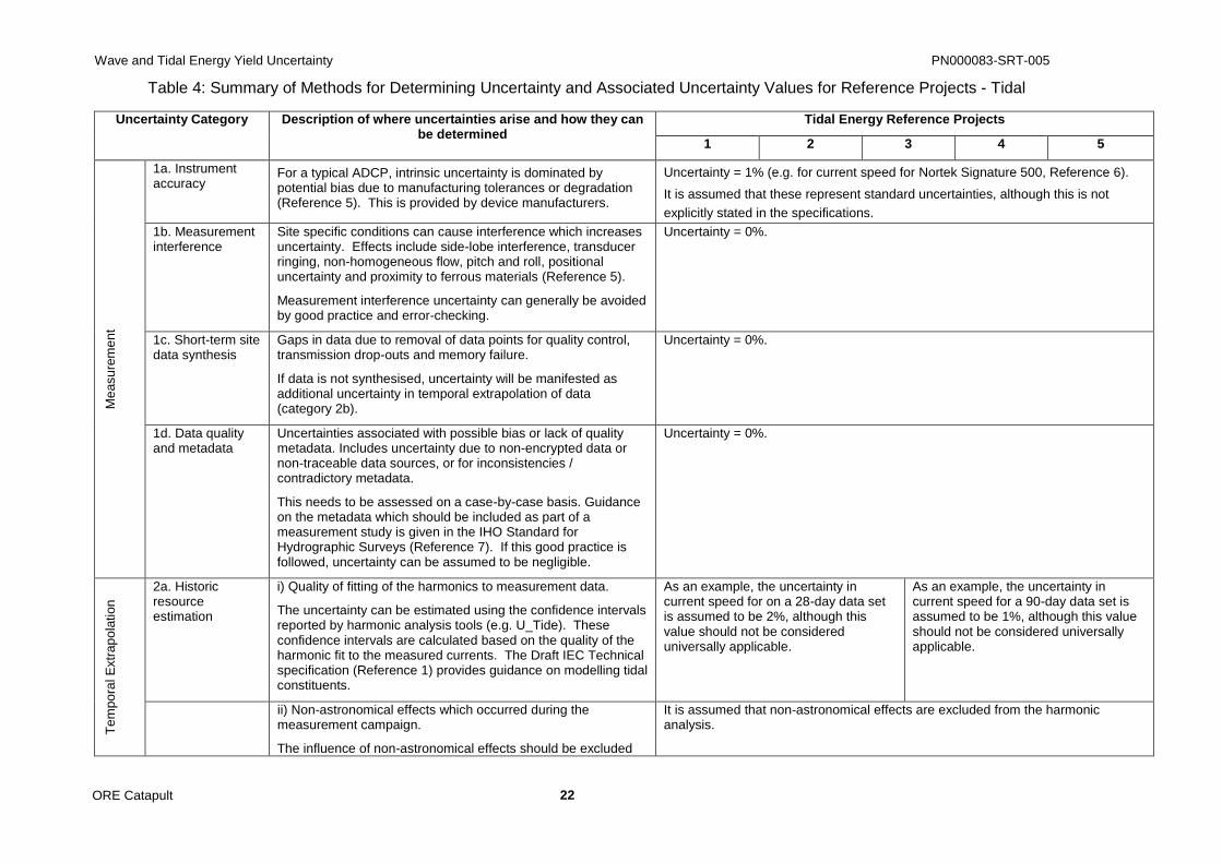
Table 4: Summary of Methods for Determining Uncertainty and Associated Uncertainty Values for Reference Projects - Tidal

Uncertainty Category Description of where uncertainties arise and how they can be determined

Tidal Energy Reference Projects

1 2 3 4 5

Me

asu

rem

en

t

1a. Instrument accuracy

For a typical ADCP, intrinsic uncertainty is dominated by potential bias due to manufacturing tolerances or degradation (Reference 5). This is provided by device manufacturers.

Uncertainty = 1% (e.g. for current speed for Nortek Signature 500, Reference 6).

It is assumed that these represent standard uncertainties, although this is not

explicitly stated in the specifications.

1b. Measurement interference

Site specific conditions can cause interference which increases uncertainty. Effects include side-lobe interference, transducer ringing, non-homogeneous flow, pitch and roll, positional uncertainty and proximity to ferrous materials (Reference 5).

Measurement interference uncertainty can generally be avoided by good practice and error-checking.

Uncertainty = 0%.

1c. Short-term site data synthesis

Gaps in data due to removal of data points for quality control, transmission drop-outs and memory failure.

If data is not synthesised, uncertainty will be manifested as additional uncertainty in temporal extrapolation of data (category 2b).

Uncertainty = 0%.

1d. Data quality and metadata

Uncertainties associated with possible bias or lack of quality metadata. Includes uncertainty due to non-encrypted data or non-traceable data sources, or for inconsistencies / contradictory metadata.

This needs to be assessed on a case-by-case basis. Guidance on the metadata which should be included as part of a measurement study is given in the IHO Standard for Hydrographic Surveys (Reference 7). If this good practice is followed, uncertainty can be assumed to be negligible.

Uncertainty = 0%.

Te

mpo

ral E

xtr

ap

ola

tion

2a. Historic resource estimation

i) Quality of fitting of the harmonics to measurement data.

The uncertainty can be estimated using the confidence intervals reported by harmonic analysis tools (e.g. U_Tide). These confidence intervals are calculated based on the quality of the harmonic fit to the measured currents. The Draft IEC Technical specification (Reference 1) provides guidance on modelling tidal constituents.

As an example, the uncertainty in current speed for on a 28-day data set is assumed to be 2%, although this value should not be considered universally applicable.

As an example, the uncertainty in current speed for a 90-day data set is assumed to be 1%, although this value should not be considered universally applicable.

ii) Non-astronomical effects which occurred during the measurement campaign.

The influence of non-astronomical effects should be excluded

It is assumed that non-astronomical effects are excluded from the harmonic analysis.


ORE Catapult 23



1 2 3 4 5

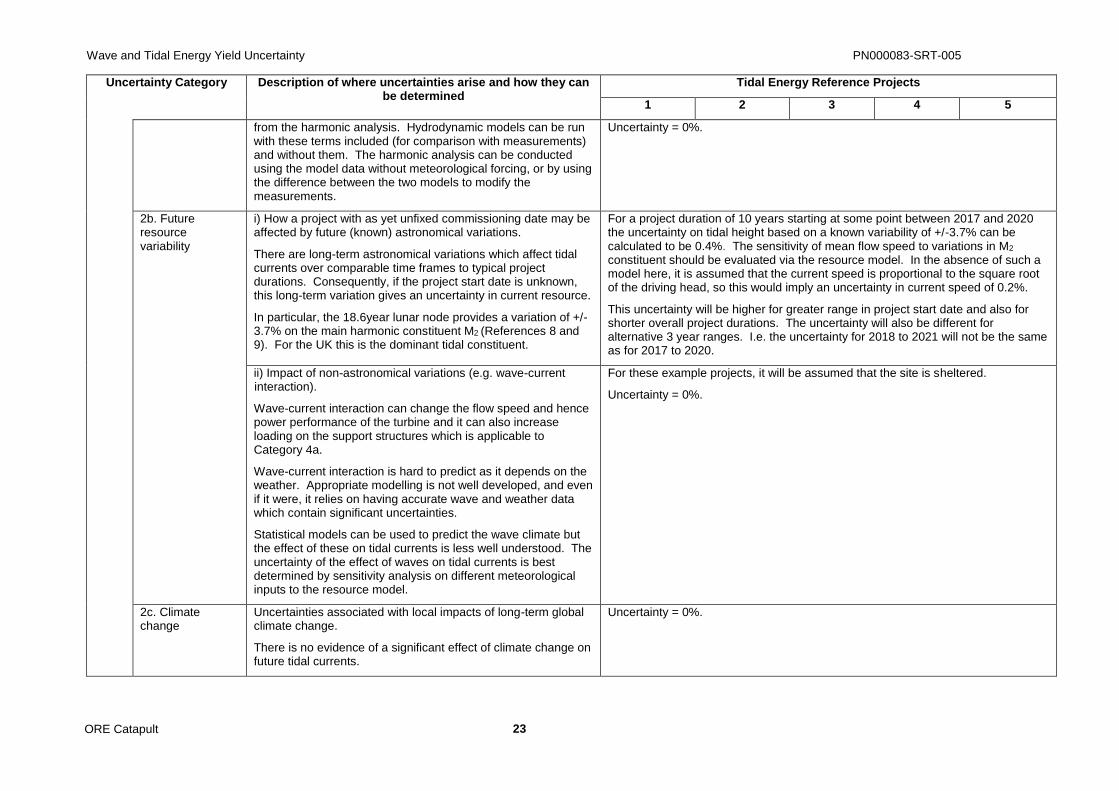
from the harmonic analysis. Hydrodynamic models can be run with these terms included (for comparison with measurements) and without them. The harmonic analysis can be conducted using the model data without meteorological forcing, or by using the difference between the two models to modify the measurements.

Uncertainty = 0%.

2b. Future resource variability

i) How a project with as yet unfixed commissioning date may be affected by future (known) astronomical variations.

There are long-term astronomical variations which affect tidal currents over comparable time frames to typical project durations. Consequently, if the project start date is unknown, this long-term variation gives an uncertainty in current resource.

In particular, the 18.6year lunar node provides a variation of +/-3.7% on the main harmonic constituent M2 (References 8 and 9). For the UK this is the dominant tidal constituent.

For a project duration of 10 years starting at some point between 2017 and 2020 the uncertainty on tidal height based on a known variability of +/-3.7% can be calculated to be 0.4%. The sensitivity of mean flow speed to variations in M2

constituent should be evaluated via the resource model. In the absence of such a model here, it is assumed that the current speed is proportional to the square root of the driving head, so this would imply an uncertainty in current speed of 0.2%.

This uncertainty will be higher for greater range in project start date and also for shorter overall project durations. The uncertainty will also be different for alternative 3 year ranges. I.e. the uncertainty for 2018 to 2021 will not be the same as for 2017 to 2020.

ii) Impact of non-astronomical variations (e.g. wave-current interaction).

Wave-current interaction can change the flow speed and hence power performance of the turbine and it can also increase loading on the support structures which is applicable to Category 4a.

Wave-current interaction is hard to predict as it depends on the weather. Appropriate modelling is not well developed, and even if it were, it relies on having accurate wave and weather data which contain significant uncertainties.

Statistical models can be used to predict the wave climate but the effect of these on tidal currents is less well understood. The uncertainty of the effect of waves on tidal currents is best determined by sensitivity analysis on different meteorological inputs to the resource model.

For these example projects, it will be assumed that the site is sheltered.

Uncertainty = 0%.

2c. Climate change

Uncertainties associated with local impacts of long-term global climate change.

There is no evidence of a significant effect of climate change on future tidal currents.

Uncertainty = 0%.


ORE Catapult 24



1 2 3 4 5 S

pa

tial E

xtr

ap

ola

tio

n

3a. Model inputs Accuracy of all data inputs to hydrodynamic or other models. Principally this comprises:

i) Bathymetry: This uncertainty can be calculated using the wave resource IEC Technical Specification (Reference 3).

ii) Bed-roughness: This is not well understood physically and is typically used as a tuning tool.

iii) Boundary conditions. The accuracy depends on the proximity to the required resource location.

The uncertainties in these inputs actually emerge in category 3b via validation of the 2D model.

N/A – measurement data available at all turbine locations. No resource modelling required.

The uncertainty associated with these effects will manifest itself in uncertainty in the model results, and hence will be picked up under category 3b. No additional uncertainty is assigned here.

Uncertainty = 0%.

3b. Horizontal and vertical extrapolation

Uncertainty in the modelling of the tidal resource between known measurement points and the turbine location(s).

There are a variety of different modelling packages which can be used to predict the spatial variation (see Section 3.1.2).

In absence of additional ADCP datasets for model validation, sensitivity analysis may be performed based on a range of different model inputs (Projects 2 and 3). It should be noted that it may be difficult to determine an appropriate range of input conditions (particularly bed roughness) and this approach may also hide the cancellation of errors. Consequently, conservative values would have to be used and uncertainty may be overstated.

Where there is an additional dataset, this may be used to validate the resource model. The primary measurement dataset is used to calibrate the model and the predictions of this model are then compared against the additional dataset. The difference between the predictions and measurements can be used to derive the uncertainty (Projects 4 and 5).

Where a 2D model is used for resource assessment, an additional uncertainty arises from the unknown shear profile. The effect of this can be quantified using a sensitivity study relating hub-height to depth-averaged flow speeds for various plausible shear profiles.

N/A – measurement data available at all turbine locations. No resource modelling required.

Spatial uncertainty (determined by sensitivity analysis) assumed to be 10%.

Without 3D CFD, there is additional uncertainty in shear profile which is assumed to be 5%.

Combining these two uncertainties in quadrature gives a total uncertainty of 11.2%.

The additional 3D CFD allows the uncertainty in shear profile to be mitigated.

Sensitivity studies result in an overall uncertainty of 10%.

The additional dataset allows CFD to be validated which reduces the uncertainty.

Uncertainty is now due to bias between model and measurements.

Uncertainty: 4% (example taken from Reference 10)

De

vic e

Pe

r

for

ma

nce 4a. Availability Device availability based on the failure rates of the devices and

the time taken to repair them. N/A –

Availability

As an example, the turbine supplier is contracted to provide an availability of 90% but in practice will aim for higher performance.


ORE Catapult 25



1 2 3 4 5

Failure rates can be obtained for generic components using standard datasets (e.g. OREDA database, Reference 11). Repair times are likely to be dominated by vessel capabilities and the metocean conditions at the site, as well as the operator’s spares strategy. For a given set of failure rates, metocean conditions and vessel capabilities, the mean availability and inter-annual variability of that availability can be calculated using a time-domain event-based Monte Carlo simulation. Sensitivity studies can them be performed to assess the sensitivity of these values to the assumed failure rates, which may differ from those in standard datasets depending on how the components are used in the device (e.g. temperature ranges and fatigue loads).

The uncertainty assigned here then comes from two factors: the uncertainty in mean availability arising from sensitivity to uncertain failure rates, and the inter-annual variability of availability.

uncertainty is managed via the turbine supply contract.

With the assumed failure rates, Monte-Carlo analysis determines the mean availability to be 93% and the inter-annual variability to be 2% for the array as a whole. Thus for a 10 year contract, this implies an uncertainty of 2/ √10 = 0.6%.

The sensitivity studies to failure rates identify a further uncertainty of 1% on availability resulting from the plausible ranges of failure rates for key components.

Combining these two uncertainties in quadrature gives a total uncertainty of 1.2%.

4b. Resource array interactions

Uncertainty associated with marine energy converter and resource interactions

i) Wake effects.

If no modelling is carried out to predict the effect of wakes, the uncertainty is defined by how much the flow of the rear turbines is expected to be affected by the front turbines (Project 2).

Wake effects are generally determined using an array planning tool (usually based on semi-empirical eddy viscosity models) or Computational Fluid Dynamics (CFD) (Projects 3-5) and the uncertainty is generally calculated by undertaking a sensitivity analysis on the wake parameters. The wake uncertainty is likely to increase with the size of array.

* assumes wake loss probability is uniformly distributed.

N/A – single turbine only.

In absence of data, it is assumed that wakes of the front three turbines reduce flow of the rear two turbines by 10%. Overall flow reduction is therefore 4%.

Uncertainty*: 4 / √3 = 2.3%.

For Projects 3 and 4 with 5 turbines this is estimated to be 1.5%.

For Project 5, there are 10 turbines and the uncertainty is estimated to be 3%.


ORE Catapult 26



1 2 3 4 5

ii) Blockage effects (large tidal only).

The IEC Technical Specification (Reference 1) states that blockage is only likely to be significant for arrays with a total power greater than 10MW. For early arrays the effect is likely to be small but this effect can be modelled using 2D depth-averaged models, 1D flow models or array modelling packages.

There is currently no way of establishing the uncertainty on these blockage estimates. For the early arrays, the blockage effect should be small so conservatively, it could be assumed that the true blockage effect lies somewhere between zero and twice the predicted value. This implies a standard uncertainty of 0.58 times the predicted blockage effect.

For larger arrays where this effect is likely to be important, it is anticipated that there will be validation data from the earlier sites.

The total power is less than 10MW and therefore blockage is insignificant.

Uncertainty = 0%.

In this example, the modelled blockage effect is assumed to be 2% so the uncertainty is 1.2%

4c. Marine energy converter power performance

i) Uncertainty within the results of full-scale performance testing (at EMEC or similar).

The methodology for full-scale testing is given in the IEC Standard (Reference 2). This also provides a list of uncertainty parameters which should be included in the assessment as a minimum. This does not specify a methodology for quantifying the overall uncertainty but this is included in the equivalent wind standard (Reference 12) and this is equally applicable to tidal energy.

For sites containing multiple devices, there will be an additional uncertainty due to variability between the devices. In the absence of relevant data to quantify this for tidal, this is judged to be around 5% between any two devices

.

N/A- managed via turbine supply contract.

As an example, this uncertainty on the performance testing is 5%*. This uncertainty is correlated across all the devices in the array, so does not reduce with increasing array size.

The additional uncertainty due to variability of performance is uncorrelated between devices so can be expressed as:

5 / √5 = 2.2%

The overall uncertainty is obtained by combining these in quadrature to give 5.5%.

* assumed uncertainty reflecting the relative immaturity of the tidal and wave industry. It is envisaged that this will decrease in time with greater validation.

For 10 turbines, the additional uncertainty due to variability of performance between the five devices is given as:

5 / √10 = 1.6%.

Overall uncertainty: 5.2%.


ORE Catapult 27



1 2 3 4 5

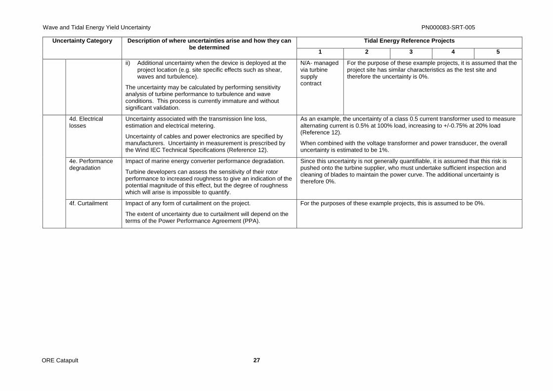
ii) Additional uncertainty when the device is deployed at the project location (e.g. site specific effects such as shear, waves and turbulence).

The uncertainty may be calculated by performing sensitivity analysis of turbine performance to turbulence and wave conditions. This process is currently immature and without significant validation.

N/A- managed via turbine supply contract

For the purpose of these example projects, it is assumed that the project site has similar characteristics as the test site and therefore the uncertainty is 0%.

4d. Electrical losses

Uncertainty associated with the transmission line loss, estimation and electrical metering.

Uncertainty of cables and power electronics are specified by manufacturers. Uncertainty in measurement is prescribed by the Wind IEC Technical Specifications (Reference 12).

As an example, the uncertainty of a class 0.5 current transformer used to measure alternating current is 0.5% at 100% load, increasing to +/-0.75% at 20% load (Reference 12).

When combined with the voltage transformer and power transducer, the overall uncertainty is estimated to be 1%.

4e. Performance degradation

Impact of marine energy converter performance degradation.

Turbine developers can assess the sensitivity of their rotor performance to increased roughness to give an indication of the potential magnitude of this effect, but the degree of roughness which will arise is impossible to quantify.

Since this uncertainty is not generally quantifiable, it is assumed that this risk is pushed onto the turbine supplier, who must undertake sufficient inspection and cleaning of blades to maintain the power curve. The additional uncertainty is therefore 0%.

4f. Curtailment Impact of any form of curtailment on the project.

The extent of uncertainty due to curtailment will depend on the terms of the Power Performance Agreement (PPA).

For the purposes of these example projects, this is assumed to be 0%.


ORE Catapult 28

Table 5: Summary of methods for determining uncertainty and associated uncertainty values for reference projects – Wave

Uncertainty Category Description of where uncertainties arise Wave Reference Projects

1 2 3

Me

asu

rem

en

t

1a. Instrument accuracy Intrinsic uncertainty of Acoustic Wave and Current Sensor (AWAC) and wave buoys is due to potential bias from manufacturing tolerances or degradation.

The calculation of the wave statistics involves additional uncertainty due to the estimation of complex parameters from a finite number of measurements. This constitutes a random scatter in the resulting estimates of significant wave height and period which reduces with the square root of the number of averaged data periods.

This information is provided by device manufacturers.

* It is assumed that these represent standard uncertainties, although this is not explicitly stated in the specifications.

Intrinsic uncertainty:

- Wave buoy uncertainty in wave height = 0.5%* (e.g. Waverider buoy, Reference 13).

- AWAC uncertainty in wave height = 1%* (e.g. Nortek AWAC, Reference 14).

The intrinsic uncertainty on the internal clock used for the energy period measurement is assumed to be negligible.

Additional uncertainty associated with wave statistical analysis: (based on averaging period of 30mins, Reference 15, and 30 day measurement period (720 averaging periods)).

- Significant wave height: 4% / √720 = 0.15%

- Energy period (Tz*) : 2% / √720 = 0.07%

*For the purpose of this example it is assumed that the uncertainty on Ts is the same as on Tz.

Overall uncertainties (added in quadrature):

Uncertainty Wave buoy (Project B): 0.52% (Hs), 0.07% (Ts)

Uncertainty AWAC (Projects C): 1.01% (Hs), 0.07% (Ts)

1b. Measurement interference

Site specific conditions can provide interference which increases uncertainty. For AWACs this is surface attenuation and spray/ air bubbles and for wave buoys this is sudden impacts and a restricted range of motion from inappropriate mooring.

For both AWACs and wave buoys, measurement interference uncertainty can generally be avoided by good practice and error-checking.

Uncertainty = 0%.

1c. Short-term site data synthesis

Gaps in data due to removal of data points for quality control, transmission drop-outs and memory failure.

If data is not synthesised, uncertainty will be manifested as additional uncertainty in temporal extrapolation of data (category 2b).

Uncertainty = 0%.


ORE Catapult 29


1 2 3

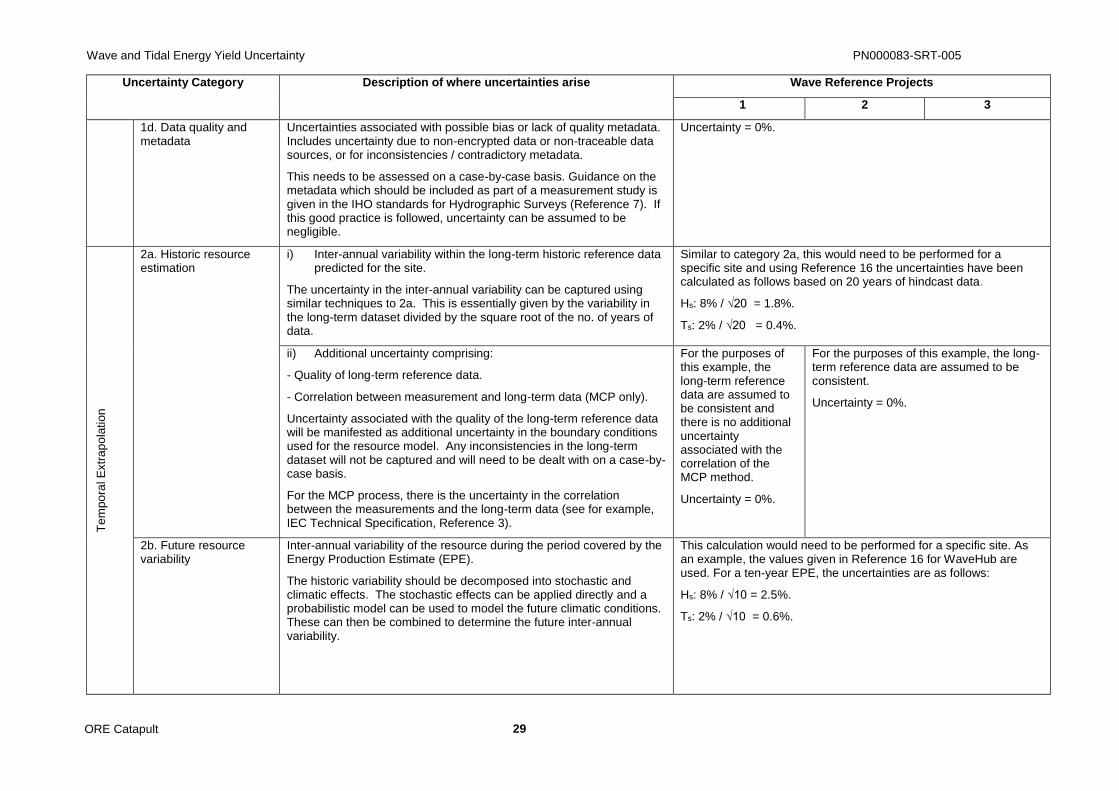
1d. Data quality and metadata

Uncertainties associated with possible bias or lack of quality metadata. Includes uncertainty due to non-encrypted data or non-traceable data sources, or for inconsistencies / contradictory metadata.

This needs to be assessed on a case-by-case basis. Guidance on the metadata which should be included as part of a measurement study is given in the IHO standards for Hydrographic Surveys (Reference 7). If this good practice is followed, uncertainty can be assumed to be negligible.

Uncertainty = 0%.

Te

mpo

ral E

xtr

ap

ola

tion

2a. Historic resource estimation

i) Inter-annual variability within the long-term historic reference data predicted for the site.

The uncertainty in the inter-annual variability can be captured using similar techniques to 2a. This is essentially given by the variability in the long-term dataset divided by the square root of the no. of years of data.

Similar to category 2a, this would need to be performed for a specific site and using Reference 16 the uncertainties have been calculated as follows based on 20 years of hindcast data.

Hs: 8% / √20 = 1.8%.

Ts: 2% / √20 = 0.4%.

ii) Additional uncertainty comprising:

- Quality of long-term reference data.

- Correlation between measurement and long-term data (MCP only).

Uncertainty associated with the quality of the long-term reference data will be manifested as additional uncertainty in the boundary conditions used for the resource model. Any inconsistencies in the long-term dataset will not be captured and will need to be dealt with on a case-by-case basis.

For the MCP process, there is the uncertainty in the correlation between the measurements and the long-term data (see for example, IEC Technical Specification, Reference 3).

For the purposes of this example, the long-term reference data are assumed to be consistent and there is no additional uncertainty associated with the correlation of the MCP method.

Uncertainty = 0%.

For the purposes of this example, the long-term reference data are assumed to be consistent.

Uncertainty = 0%.

2b. Future resource variability

Inter-annual variability of the resource during the period covered by the Energy Production Estimate (EPE).

The historic variability should be decomposed into stochastic and climatic effects. The stochastic effects can be applied directly and a probabilistic model can be used to model the future climatic conditions. These can then be combined to determine the future inter-annual variability.

This calculation would need to be performed for a specific site. As an example, the values given in Reference 16 for WaveHub are used. For a ten-year EPE, the uncertainties are as follows:

Hs: 8% / √10 = 2.5%.

Ts: 2% / √10 = 0.6%.


ORE Catapult 30


1 2 3

2c. Climate change Uncertainties associated with local impacts of long-term global climate change.

There is no significant evidence of the effect of climate change on future wave climates.

Uncertainty = 0%.

Sp

atial E

xtr

ap

ola

tio

n

3a. Model inputs Accuracy of all data inputs to hydrodynamic or other models. Principally this comprises:

(i) Bathymetry: uncertainty can be calculated using the IHO survey Standard (Reference 7).

(ii) Wave data at model boundaries: Generally derived from larger-scale reanalysis datasets which are known to have certain biases (Reference 17).

(iii) Meteorological data inside the model domain.

(iv) Tide height.

The uncertainties in these inputs actually emerge in category 3b via validation of the 2D model and hence can be picked up under category 3b.

N/A- spatial extrapolation uncertainties are not applicable for the MCP method.

No additional uncertainty is assigned here.

Uncertainty = 0%.

3b. Horizontal and vertical extrapolation

Models are used to propagate waves from model boundary conditions to the device location and there is uncertainty in the mean resource prediction.

Third generation models such as SWAN capture all the physical effects relevant to this propagation and are recommended in the IEC Technical Specification (Reference 3). The uncertainty should be determined by comparing site measurements with model predictions.

N/A - spatial extrapolation uncertainties are not applicable for the MCP method.

The uncertainty would be evaluated on a site-specific basis. Uncertainties on wave period are likely to be higher than on wave height, and uncertainties are likely to be greater nearshore than further offshore. For the purposes of this example, the following uncertainties are assigned:

For Projects B.2 and B.3, 10% uncertainty on Hs and 15% uncertainty on Te.

For projects C.2 and C.3, 15% uncertainty on Hs and 20% uncertainty on Te.

Devic

e

Pe

rfo

rma

n

ce

4a. Availability The approach taken here is the same as that for tidal turbines. The values assigned here are likely to be greater because the technology is less mature and the extreme loads that a wave device has to survive are so much greater than the normal operating loads.

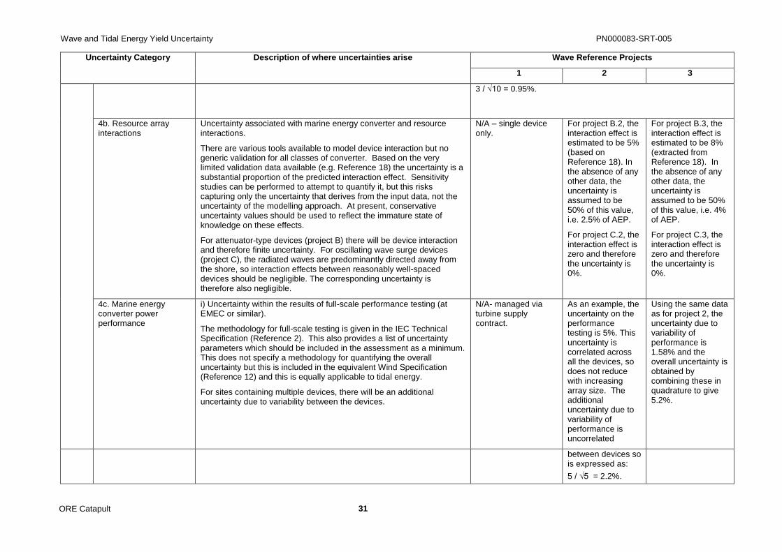
As an example, the turbine supplier is contracted to provide an availability of 85% but in practice will aim for higher performance. Monte-Carlo analysis determines the mean availability to be 90% and the uncertainty to be 3% per year.

For a ten-year EPE, this implies an uncertainty of


ORE Catapult 31


1 2 3

3 / √10 = 0.95%.

4b. Resource array interactions

Uncertainty associated with marine energy converter and resource interactions.

There are various tools available to model device interaction but no generic validation for all classes of converter. Based on the very limited validation data available (e.g. Reference 18) the uncertainty is a substantial proportion of the predicted interaction effect. Sensitivity studies can be performed to attempt to quantify it, but this risks capturing only the uncertainty that derives from the input data, not the uncertainty of the modelling approach. At present, conservative uncertainty values should be used to reflect the immature state of knowledge on these effects.

For attenuator-type devices (project B) there will be device interaction and therefore finite uncertainty. For oscillating wave surge devices (project C), the radiated waves are predominantly directed away from the shore, so interaction effects between reasonably well-spaced devices should be negligible. The corresponding uncertainty is therefore also negligible.

N/A – single device only.

For project B.2, the interaction effect is estimated to be 5% (based on Reference 18). In the absence of any other data, the uncertainty is assumed to be 50% of this value, i.e. 2.5% of AEP.

For project C.2, the interaction effect is zero and therefore the uncertainty is 0%.

For project B.3, the interaction effect is estimated to be 8% (extracted from Reference 18). In the absence of any other data, the uncertainty is assumed to be 50% of this value, i.e. 4% of AEP.

For project C.3, the interaction effect is zero and therefore the uncertainty is 0%.

4c. Marine energy converter power performance

i) Uncertainty within the results of full-scale performance testing (at EMEC or similar).

The methodology for full-scale testing is given in the IEC Technical Specification (Reference 2). This also provides a list of uncertainty parameters which should be included in the assessment as a minimum. This does not specify a methodology for quantifying the overall uncertainty but this is included in the equivalent Wind Specification (Reference 12) and this is equally applicable to tidal energy.

For sites containing multiple devices, there will be an additional uncertainty due to variability between the devices.

N/A- managed via turbine supply contract.

As an example, the uncertainty on the performance testing is 5%. This uncertainty is correlated across all the devices, so does not reduce with increasing array size. The additional uncertainty due to variability of performance is uncorrelated

Using the same data as for project 2, the uncertainty due to variability of performance is 1.58% and the overall uncertainty is obtained by combining these in quadrature to give 5.2%.

between devices so is expressed as:

5 / √5 = 2.2%.


ORE Catapult 32


1 2 3

The overall uncertainty is obtained by combining these in quadrature to give 5.5%.

ii) Additional uncertainty when the device is deployed at the project location (e.g. site specific effects such as shear, waves and turbulence).

The uncertainty may be calculated by performing sensitivity analysis of turbine performance to turbulence and wave conditions. This process is currently immature and without significant validation.

For the purpose of these example projects, it is assumed that the project site has similar characteristics as the test site and therefore the uncertainty is 0%.

4d. Electrical losses Uncertainty associated with the transmission line loss, estimation and electrical metering.

Uncertainty of cables and hubs are specified by manufacturers. Uncertainty in measurement is prescribed by the Wind Industry IEC Technical Specifications (Reference 12).

Similar to tidal, the uncertainty is estimated to be 1%.

4e. Performance degradation

Impact of marine energy converter performance degradation.

Wave energy convertors have more in common with other marine structures (e.g. oil & gas platforms) than tidal turbines, as they generally act as Morison elements in the flow rather than lifting surfaces. Oil and gas standards (e.g. References 19 and 20) can therefore be used to quantify the potential impact of marine growth on device mass and dimensions. WEC performance models can then be used to convert this into an effect on power performance. Sensitivity studies on this process allow the uncertainty to be evaluated.

It is assumed that this risk is pushed onto the turbine supplier, who must build in sufficient design margin and/or undertake sufficient inspection and cleaning of devices to maintain the power matrix. The additional uncertainty is therefore 0%.

4f. Curtailment Impact of any form of curtailment on the project.

The extent of uncertainty due to curtailment will depend on the terms of the Power Performance Agreement (PPA).

The uncertainty is assumed to be 0%.


ORE Catapult 33

6 Conclusions

The assessment of uncertainty in wave and tidal energy yield predictions is relatively immature,

although is becoming increasing important as investment is sought by the industry.

This document provides guidance for determining project uncertainties based on the taxonomy

document of individual uncertainty categories. It has been developed from a literature review

and stakeholder engagement process, and as such, represents a snapshot of the current state-

of-the-art. This field is evolving rapidly and the guidance given herein may be superseded by

ongoing or future research and/or operational experience with early arrays.

This guidance has been applied to a series of example projects to highlight variations in

approach and overall uncertainties which can arise from different types and sizes of project. By

understanding how uncertainty is affected by different modelling or measurement approaches, it

is envisaged that project developers will be better able to make decisions on how to undertake

EPEs for wave and tidal energy projects.

There are a number of categories which are difficult to quantify and this has highlighted

potential follow-on work to improve the assessment of uncertainty. In particular, this includes:

Wave-current interaction (tidal and wave categories 2a, 2b).

Spatial extrapolation of measurement data across a resource (tidal and wave 3a, 3b).

Power curve adjustments for potential project sites (wave and tidal, category 4c) and the

degradation of those power curves due to marine growth (tidal and wave, category 4d).

Availability of power (tidal and wave, category 4a).


ORE Catapult 34

7 References

1. Marine Energy – Wave, Tidal and Other Water Current Converters – Part 201: Tidal Energy Resource Assessment and Characterization, IEC Draft Technical Specification 62600-201, 2014.

2. Marine Energy – Wave, Tidal and Other Water Current Converters – Part 200: Electricity Producing Tidal Energy Converters - Power Performance Assessment, IEC Technical Specification 62600-200: 2013.

3. Marine Energy – Wave, Tidal and Other Water Current Converters – Part 101: Wave Energy Resource Assessment and Characterization, IEC Draft Specification 62600-101, 2014.

4. Marine Energy – Wave, Tidal and Other Water Current Converters – Part 100: Electricity Producing Wave Energy Converters - Power Performance Assessment, IEC Draft Technical Specification 62600-100: 2013.

5. ADCP Principles of Operation, a Practical Primer, Teledyne RD Instruments, January 2011.

6. Nortek Signature 1000/500 Datasheet, Nortek.

7. IHO Standards for Hydrographic Surveys, International Hydrographic Bureau, 5th Edition, Special Publication no. 44, 2008.

8. Tidal Analysis and Prediction, B. Parker, NOAA Special Publication NOS CO-OPS, July 2007.

9. Tides, Surges and Mean Sea-level, D. Pugh, John Wiley and Sons, 1996.

10. EIC/ Renewables-PN11260: ETI ReDAPT – MA1001 PM14 MD5.2: Falls of Warness 3D Model Validation Report, K. Gunn, 2014.

11. OREDA (Offshore Reliability Data) Handbook, 5th Edition, Volume I and II, 2009.

12. IEC 61400-12-1: Wind Turbines – Part 12-1: Power Performance Measurements of Electricity Producing Wind Turbines.

13. Directional Waverider MkIII Technical Specification, Datawell – Oceanographic Instruments.

14. AWAC technical specification, Nortek.

15. Variability of Calculated Wave Parameters, Datawell- Oceanographic Instruments.

16. Defining the Long-term Wave Resource at Wave Hub: The Role of Measurements and Models, J. Philip et al., Garrad Hassan and Partners Ltd, Proceedings of the AMSE 27th International Conference on Offshore Mechanics and Arctic Engineering, 2008 (OMA2008-57349).

17. The ERA-interim Reanalysis: Configuration and Performance of the Data Assimilation System, D. Dee et al., Quarterly Journal of the Royal Meteorological Society, Vol. 137, 2011.

18. Validation of Design and Planning Tools for Wave Energy Converters (WECs), J. Cruz et al., Proceedings of the 1st Marine Energy Technology Symposium, METS13, Washington, 2013.

19. Petroleum and Natural Gas Industries – Specific Requirements for Offshore Structures – Part 1: Metocean Design and Operating Considerations, ISO 19901-1: 2005.

20. Environmental Care, Norsok Standard S-003, Rev 3, December 2005.


ORE Catapult 35

8 Acknowledgements

The authors would like to thank the following organisations for their participation in the

stakeholder engagement component of this project:

Alstom

Andritz

ANSYS

Atlantis Resources

Carnegie Wave Evergy

Cranfield University

Deltares

DHI

DNV-GL

DP Energy (OREC Yield TWG)

E.ON

EDF R&D

GDF Suez

MeyGen (OREC Yield TWG)

NAREC

NaturalPower

Nortek International

Nova Innovation

Partrac

Queen's University Belfast

RES

RS Aqua

SAMS

Schottel

ScottishPower Renewables (OREC Yield TWG)

SgurrEnergy

SSE

Teledyne DR Instruments

The Crown Estate

Tidal Energy Ltd (TEL)

Tocardo

UHI - ERI Thurso

UHI - Lewis

University of Cambridge

University of Edinburgh

University of Exeter

University of Hull

University of Manchester

University of Oxford

University of Strathclyde


ORE Catapult 36

Annex A

Screen-shot of the Interactive Uncertainty Tool developed as part of this project and used to

determine the overall uncertainties of the example projects in Section 4.


ORE Catapult 37

Contact ORE Catapult Inovo 121 George Street Glasgow, G1 1RD

T +44 (0)333 004 1400 F +44 (0)333 004 1399

ORE Catapult National Renewable Energy Centre Offshore House Albert Street, Blyth Northumberland, NE24 1LZ

T +44 (0)1670 359 555 F +44 (0)1670 359 666

[email protected] Ore.catapult.org.uk

Documents

Wave and Tidal Energy Yield Uncertainty - ORE Catapult · 2018-01-23 · Tidal energy is essentially deterministic (driven by the position of the sun and moon relative to the earth),