Applied Scientific Research 47: 273-285, 1990.

~© 1990 Kluwer Academic Publishers. Printed in the Netherlands.

W a t e r h a m m e r with f luid-structure interact ion

A.S. TIJSSELING I & C.S.W. LAVOOIJ 2

1Department of Civil Engineering, Delft University of Technology, Delft, 2Industrial Hydrodynamics and Dredging Technology Division, DELFT HYDRAULICS, Delft, The Netherlands

Received 18 April 1989; accepted in revised form 10 March 1990

Abstract. The classical theory of waterhammer is a well-known and accepted basis for the prediction of

pressure surges in piping systems. In this theory the piping system is assumed not to move. In practice

however piping systems move when they are loaded by severe pressure surges, which for instance occur after rapid valve closure or pump failure. The motion of the piping system induces pressure surges which are not

taken into account in the classical theory.

In this article the interaction between pressure surges and pipe motion is investigated. Three interaction

mechanisms are distinguished: friction, Poisson and junction coupling. Numerical experiments on a single

straight pipe and a liquid loading line sho W that interaction highly influences the extreme pressures during waterhammer occurrences.

Nomenclature

A s = cross-sectional discharge area A~ = cross-sectional pipe wall area

c z = pressure wave speed in fluid c~ = axial stress wave speed in pipe wall

E = Young's modulus for pipe wall material e = pipe wall thickness

f = Darch-Weisbach friction coefficient g = gravitational acceleration

H = fluid pressure head h = elevation of pipe

Ky = fluid bulk modulus

P = fluid pressure

R = internal radius of pipe

Tc -: valve closure time

t = time

u r = radial displacement of pipe u~ = axial displacement of pipe

h z = axial velocity of pipe V = fluid velocity

z = distance along pipe

7 = elevation angle of pipe

)o = length of pressure wave v = Poisson's ratio

Py = fluid density Pt = density of pipe wall material

a~ = axial pipe stress

% = hoop stress

1. Introduction

When in a fluid-filled piping system under stationary flow conditions at some location the fluid velocity changes, pressure surges are induced which propagate at speed c I through the system. Spectacular pressure surges, referred to as waterhammer, can be caused by e.g. rapid valve closure, pump failure or cavity collapse. The maximum pressure rise or drop AP due to a velocity change AV can be estimated by Joukowsky's formula [1]:

A P = PsCs AK (1)

274 A.S. Tijsseling and C.S.W. Lavoo(/

in which pf is the density of the fluid. To give an example, in a steel pipe filled with water (pz = 1000 kg/m 3) the pressure wave speed is about 1000 m/s. A relatively small change in the flow velocity (0.1 m/s) leads here to a relatively high change in the pressure (105 N/m 2 = 1 bar).

In designing piping systems it is usual to perform waterhammer calculations in order to predict extreme pressures and reaction forces in emergency situations. From the calculated results the dimensions of the piping system are determined and it is judged whether devices like relieve valves are necessary.

Sometimes one is interested in the dynamic behaviour of the piping system. This in order to determine accurately reaction forces, stresses and resonance frequencies. Often an uncoupled calculation is carried out. With classical waterhammer theory [7] pressure histories are calculated which serve as input for a structural code that simulates the dynamic behaviour of the piping system. The calculation is called uncoupled since the motion of the piping system is unable to influence the pressures in the fluid. The question arises whether this influence of pipe motion on fluid pressures may be neglected. In other words: Is fluid-structure interaction (FSI) important?

In this article FSI is studied from some simple examples. The mechanisms causing FSI are outlined. The mathematical model and solution procedures underlying the numerical results are shortly described. Calculations are performed on the DELFT HYDRAULICS benchmark problems A and F [8]. Problem A is a simple reservoir- pipe-valve system, problem F represents a liquid loading line as used in practice. Uncoupled calculations are compared with calculations including FSI.

The work presented in this article is based on that of many other investigators. Most of them are referred to in a review paper of Wiggert, published in 1986 [6].

2. Fluid-structure interaction

Three mechanisms are distinguished which couple the dynamic behaviour of fluid and piping system: (1) friction coupling, (2) Poisson coupling and (3)junction coupling. Friction and Poisson coupling act along the entire piping system, junction coupling only at specific places such as elbows, tees or valves.

2.1. Friction couplin9

Friction coupling represents the mutual friction between fluid and pipe. It is of less

importance for the dynamic problems in this article.

2.2. Poisson coupling

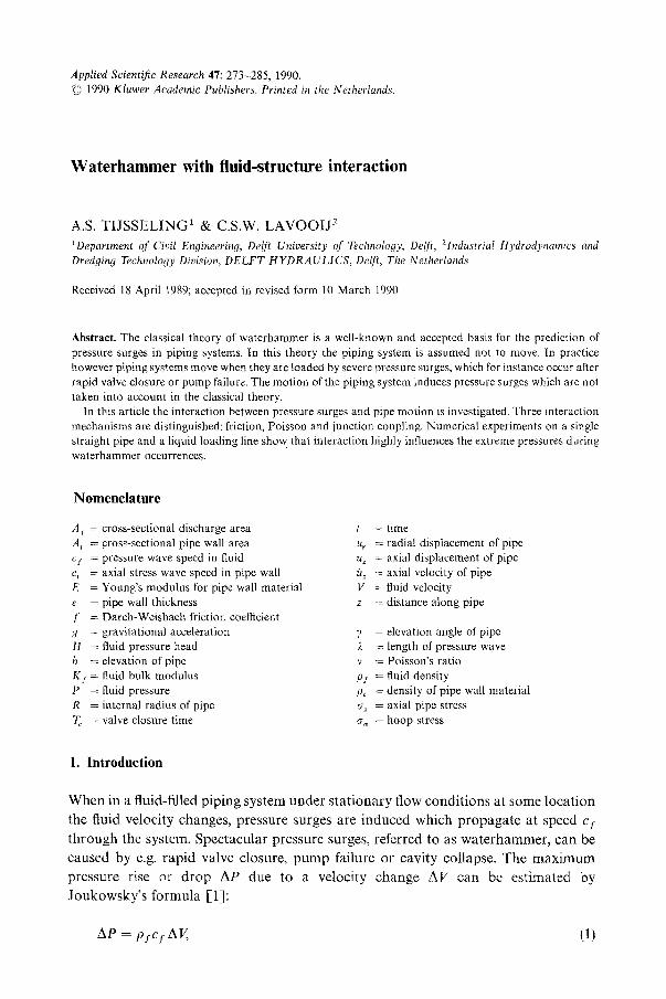
Poisson coupling relates the pressures in the fluid to the axial stresses in the pipe via the contraction or expansion of the pipe wall. The mechanism of Poisson coupling is illustrated in Fig. 1. In Fig. la fluid is flowing at velocity V and reference pressure

(a) t Waterhammer with fluid-structure interaction

pipe wa]]

V

- - ~ ' - - - - f l u i d

P = 0

275

(b)

c t = [ f ] u i d p r e s s u r e

cf t ct ~ i]l /

(c) t " " - - f l u i d

[

Fig. 1. Poisson coupling.

pipe w a l l (exaggerateO)

P = 0. In Fig. lb the fluid is stopped instantaneously, resulting in a pressure rise which

propagates at speed c I through the fluid. The pressure rise is accompanied by a radial expansion of the pipe wall as shown in Fig. lc. Due to this radial expansion the pipe

shortens behind and elongates in front of the pressure rise. The elongation reveals itself as an axial stress wave. It propagates at speed ct through the pipe and causes a

radial contraction of the pipe wall (see Fig. lc). The radial contraction causes a secondary pressure rise in the fluid as shown in Fig. 1 b. This secondary pressure rise is

often referred to as precursor wave since it propagates at speed c,, which is generally higher than the propagation speed c I of the primary pressure rise.

p cf cf_ l cf

(a) (b)

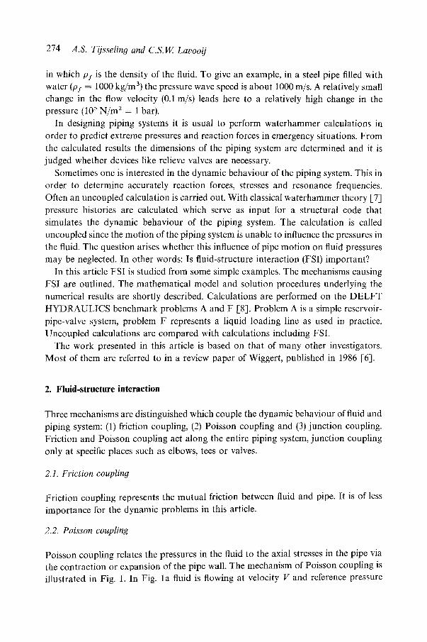
Fig. 2. Junction coupling.

276 A.S. Tijsseling and C.S.W. Lavooq

2.3. Junction coupling

Junction coupling describes local forces acting mutually between fluid and piping system. An example is given in the forthcoming. Consider a pipe bridge as shown in Fig. 2. When a pressure wave has passed the elbow on the right (Fig. 2a), the net pressure difference between the two elbows causes the pipe bridge to move (Fig. 2b). Due to the motion the pressure drops at the right and rises at the left elbow, as shown simplified in Fig. 2b. The motion of the pipe bridge induces pressure waves in the fluid, which in return influence the motion of the bridge.

3. Mathematical model

The utilized mathematical model is essentially one-dimensional, corresponding to classical waterhammer and beam theory. New is the coupling between fluid and piping system. A four equations model describing the dynamic behaviour of a straight fluid-filled pipe is presented. Friction, Poisson and junction coupling are taken into account. The pipe can move only in the axial direction. The lateral and rotational motion of the pipe are not considered here.

3. l. Assumptions

For the fluid it is assumed that the long wave length (2 >> R) and the acoustic (cy >> V) approximation are valid. The friction is modelled as if the flow were steady and cavitation is assumed not to occur. The pipe is assumed to be prismatic and thin walled. It behaves linearly elastically and inertia in radial direction is neglected.

3.2. Equations for the .fluid

The fluid is described by its velocity V and pressure head H (H=P/(p/g)+h). Two equations for V and H are provided by the momentum balance

c3V cgH f + goz-z = - ~4~(V - h~)lV - h~l (2) F

and the mass balance

OV g OH OG + - 2v (3)

8z cZv 8t 8z

in which

{ (K17r 2R(1--v2))} -~/2. C F = p f -{- __ e E

(4)

Waterhammer with f luid-structure interaction 277

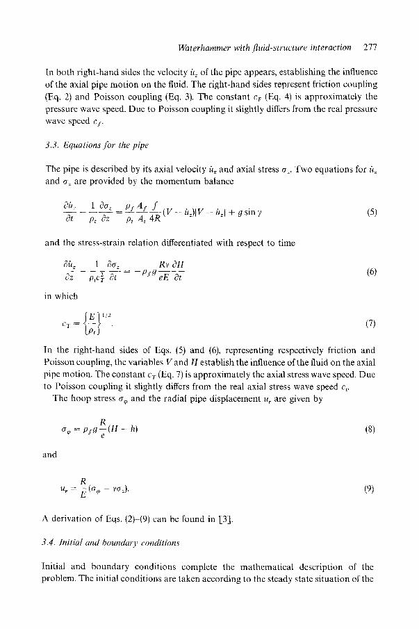
In both right-hand sides the velocity/~z of the pipe appears, establishing the influence of the axial pipe motion on the fluid. The right-hand sides represent friction coupling (Eq. 2) and Poisson coupling (Eq. 3). The constant c v (Eq. 4) is approximately the pressure wave speed. Due to Poisson coupling it slightly differs from the real pressure wave speed c I.

3.3. Equations f o r the pipe

The pipe is described by its axial velocity/~= and axial stress %. Two equations for/~= and a= are provided by the momentum balance

Oit~ 1 Oa~_ P F A f f

~t Pt ~Z Pt At 4R (V - ~)l V -/~zl + g sin 7

and the stress-strain relation differentiated with respect to time

(5)

in which

~ E ; 1/2 cr -- - - (7)

( P t ) "

In the right-hand sides of Eqs. (5) and (6), representing respectively friction and Poisson coupling, the variables V and H establish the influence of the fluid on the axial pipe motion. The constant Cr (Eq. 7) is approximately the axial stress wave speed. Due to Poisson coupling it slightly differs from the real axial stress wave speed %

The hoop stress a~, and the radial pipe displacement u r are given by

R a r = p e g - - ( H - h) (8)

e

and

R u, = ~ (% - va~). (9)

A derivation of Eqs. (2)-(9) can be found in [3].

3.4. Initial and boundary conditions

Initial and boundary conditions complete the mathematical description of the problem. The initial conditions are taken according to the steady state situation of the

~h z 1 aaz Rv OH & pt c2 8t - P Y g e E & (6)

278 A.S. Tijsselin9 and C.S.W. Lavooij

system. The boundary conditions describe the situation at the pipe's ends, where for instance a reservoir or valve is located. Junction coupling is modelled via the boundary conditions.

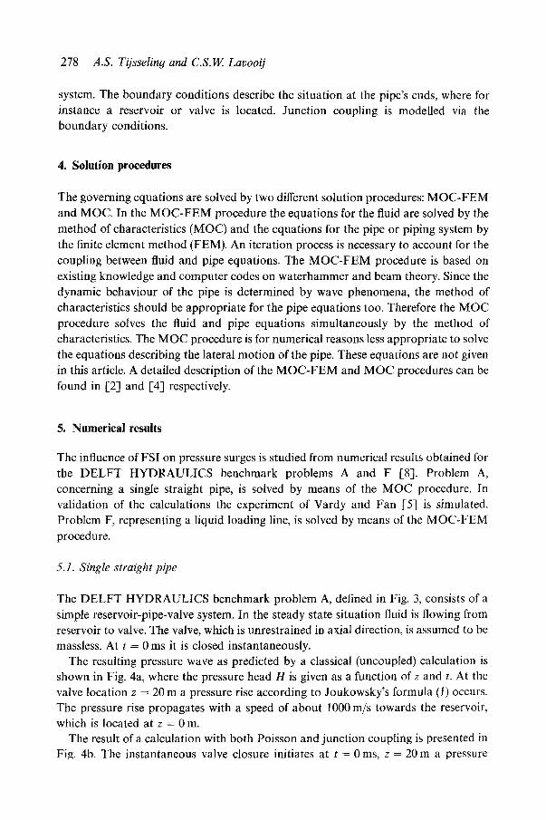
4. Solution procedures

The governing equations are solved by two different solution procedures: MOC-FEM and MOC. In the MOC-FEM procedure the equations for the fluid are solved by the method of characteristics (MOC) and the equations for the pipe or piping system by the finite element method (FEM). An iteration process is necessary to account for the coupling between fluid and pipe equations. The MOC-FEM procedure is based on existing knowledge and computer codes on waterhammer and beam theory. Since the dynamic behaviour of the pipe is determined by wave phenomena, the method of characteristics should be appropriate for the pipe equations too. Therefore the MOC procedure solves the fluid and pipe equations simultaneously by the method of characteristics. The MOC procedure is for numerical reasons less appropriate to solve the equations describing the lateral motion of the pipe. These equations are not given in this article. A detailed description of the MOC-FEM and MOC procedures can be found in [2] and [4] respectively.

5. Numerical results

The influence of FSI on pressure surges is studied from numerical results obtained for the D E L F T HYDRAULICS benchmark problems A and F [8]. Problem A, concerning a single straight pipe, is solved by means of the MOC procedure. In validation of the calculations the experiment of Vardy and Fan [5] is simulated. Problem F, representing a liquid loading line, is solved by means of the MOC-FEM

procedure.

5.1. Single straight pipe

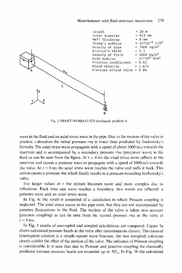
The D E L F T HYDRAULICS benchmark problem A, defined in Fig. 3, consists of a simple reservoir-pipe-valve system. In the steady state situation fluid is flowing from reservoir to valve. The valve, which is unrestrained in axial direction, is assumed to be massless. At t = 0 ms it is closed instantaneously.

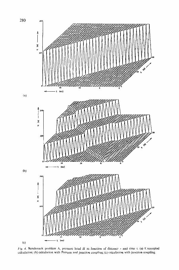
The resulting pressure wave as predicted by a classical (uncoupled) calculation is shown in Fig. 4a, where the pressure head H is given as a function of z and t. At the valve location z = 20 m a pressure rise according to Joukowsky's formula (1) occurs. The pressure rise propagates with a speed of about 1000 m/s towards the reservoir, which is located at z = 0 m.

The result of a calculation with both Poisson and junction coupling is presented in Fig. 4b. The instantaneous valve closure initiates at t = 0 ms, z = 20 m a pressure

Waterhammer with fluid-structure interaction 279

Length = Outer diameter = Wall thickness = Young ' s modulus = Density of pipe =

I Po~sson' s ratio = h I

~.~ ~ Density of fluid ~d~ ~ B u l k modulus

~.I ~ Friction coefficient ~ Fluid velocity

-A ~ ~ P r e s s u r e behind valve

B

20 In 813 mm 8 mrs 21-]01° N/rn 2 7900 kg/m 3 0.3 1000 kg/m ~ 21-10 e N/m 2 0.02 1 m/s 0 p a

Fi 9. 3. DE L F T HYDRAULICS benchmark problem A.

wave in the fluid and an axial stress wave in the pipe. Due to the motion of the valve in

positive z-direction the initial pressure rise is lower than predicted by Joukowsky's

formula. The axial stress wave propagates with a speed of about 5000 m/s towards the

reservoir and is accompanied by a secondary pressure rise (precursor wave) in the

fluid as can be seen from the figure. At t -- 4 ms the axial stress wave reflects at the

reservoir and causes a pressure wave to propagate with a speed of 1000 m/s towards

the valve. At t = 8 ms the axial stress wave reaches the valve and pulls it back. This

action causes a pressure rise which finally results in a pressure exceeding Joukowsky's value.

For larger values of t the picture becomes more and more complex due to

reflections. Each time one wave reaches a boundary, two waves are reflected: a

pressure wave and an axial stress wave,

In Fig. 4c the result is presented of a calculation in which Poisson coupling is

neglected. The axial stress waves in the pipe exist, but they are not accompanied by

pressure fluctuations in the fluid. The motion of the valve is taken into account

(junction coupling) as can be seen from the second pressure rise at the valve at t = 8 m s .

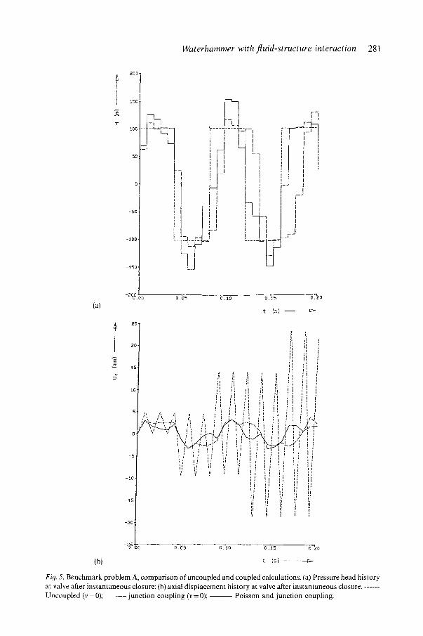
In Fig. 5 results of uncoupled and coupled calculations are compared. Figure 5a shows calculated pressure heads at the valve after instantaneous closure. The classical

(uncoupled) solution is a simple square wave function, the new (coupled) solutions

clearly exhibit the effect of the motion of the valve. The influence of Poisson coupling

is considerable. It is seen that due to Poisson and junction coupling the classically

predicted extreme pressure heads are exceeded up to 50%. In Fig. 5b the calculated

280

10{

(a)

(b)

2O

~0 ,t, ~ '~

15 1o 5 0

-.m t {ms)

E

t5 10 5

t (ms)

/"

o 15 io 5 o

- '~ t {ms) (c)

Fiq. 4. Benchmark problem A, pressure head H as function of distance z and time t. (a) Uncoupled calculation; (b) calculation with Poisson and junction coupling; (c) calculation with junction coupling.

Waterhammer with fluid-structure interaction 281

(a)

I

200 "

150R

100

50

0

-50

-100

-150

. . . . . ~ Z Z F 7 [_', I

- 1 I

I

' I

-1o

-d5

-20

(b)

F7

-20~ ; u . oo 0.05 O. I0 0 .'~5 o '.'.~ 0

~5

~0

~0

f i

0

15 .

t I s ) - - ~'

h t , I l! I I

, i ' 1 ' , , , , i i

, t ' t ' i , I , i I i I I * '

J , J , ~ , i i i , , , , L ' i ' , , , I

,/;, ; ' , /i ~ ;~ ; ! ' ! , I i , ; i ~ , ' ,"

i ' , ' I , , ' , 4 ' , , , ' ' ' L '

l I L ' . 1 , ; ; J j ' ' , , ' I r

V ~i it ~ ~' I , r , '

, , i

i ! l I i ,i ; J

!1 ~ ' i ' , ,, , i (

I~ 'i ,i

O. 05 0. lO

t (sl

Fig. 5. Benchmark problem A, comparison of uncoupled and coupled calculations. (a) Pressure head history at valve after instantaneous closure; (b) axial displacement history at valve after instantaneous closure. - . . . . . Uncoupled (v = 0); - - - j u n c t i o n coupling (v = 0); - - Poisson and junction coupling.

282 A.S. Tijsseling and C.S.W. Lavvoij

L I - - - - - - ' - I l z

2 o !

II / 3 ! / -3DO I , , - L~ ,

0 2 4 6 B 4_0

"G

.Y

I I

2 ~ E, B IO

300

150

0

-152.'

-300 •

0

J

2 4 6 6 10 0 2 LI 6 B I0

300

150

0

-150

-300

I

O,

i-Y

6 B 10 2 4 6 B

t {ms] ~, t (mS]

10

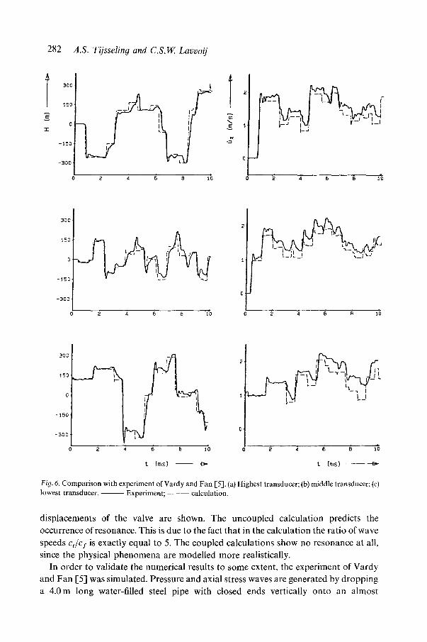
Fig. 6. Comparison with experiment of Vardy and Fan [5]. (a) Highest transducer; (b) middle transducer; (c) lowest transducer. Experiment; . . . . . calculation,

displacements of the valve are shown. The uncoupled calculation predicts the occurrence of resonance. This is due to the fact that in the calculation the ratio of wave speeds cJc s is exactly equal to 5. The coupled calculations show no resonance at all, since the physical phenomena are modelled more realistically.

In order to validate the numerical results to some extent, the experiment of Vardy and Fan [5] was simulated. Pressure and axial stress waves are generated by dropping a 4.0 m long water-filled steel pipe with closed ends vertically onto an almost

Waterhammer with fluid-structure interaction 283

immovable base. The height of free fall is 49.7 mm. At five locations along the pipe, which has an internal diameter of 53.5 mm and a wall thickness of 3.6 ram, dynamic pressures and pipe accelerations were measured. The pipe velocities were derived from the measured accelerations by integration. The measured pressure heads and axial pipe velocities at the lowest, middle and highest location just after impact are shown in Fig. 6, together with calculated results. The agreement between measurements and calculations is reasonable. The measured wave speeds were 1360 _+ 19 m/s for the pressures and 5190 _+ 20 m/s for the axial stresses, the corresponding calculated wave speeds are 1351 m/s and 5159 m/s. The precursor wave is recognized in Fig. 6b as a negative pressure change existing before the arrival of the main pressure wave at t = 1.5 ms. It is noted that in the calculations the gravitational acceleration and the masses of the pipe's end caps are neglected.

5.2. Liquid loading line

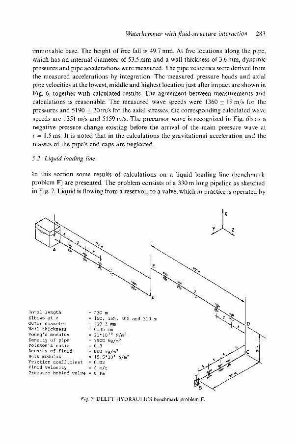
In this section some results of calculations on a liquid loading line (benchmark problem F) are presented. The problem consists of a 330 m long pipeline as sketched in Fig. 7. Liquid is flowing from a reservoir to a valve, which in practice is operated by

Total length Elbows at z =

Outer diameter =

Wall thickness

Young's modulus =

Density of pipe =

Po[sson's ratio =

Density of fluid =

Bulk modulus =

Friction coefficient =

Fluid velocity =

Pressure behind valve =

330 m

150, 155, 305 and 310 m

219.1 mm 6.35 mm 21"101° N/m 2

7900 kg/m 3

0.3

880 kg/m ~

15.5"108 N/m ~

0.02

4 m/s 0 Pa

Fig. 7. DELFT HYDRAULICS benchmark problem F.

2 8 4 A.S. Tijsseling and C.S.W. Lavooij

(a)

t

J & o_

D-

4"

2

0__/ - 2

ii0

!

I / , 4 ; /i i / / ~ : / I

:~ "F, i

i /J ; V ] '~ . . . . - -

i

0 . 5 42D 1 .5 2 . 0 2 . 5

t ( s l

37o

- 2

-4 .

/ ' x i / % ,

[ I \

,, ,' ',

; I l

' \ I

:: ,'%j/ i !

/

-I~.'o o.'5 ~o ~5 2~o 2~5 ~:o

(b ) t Csl >

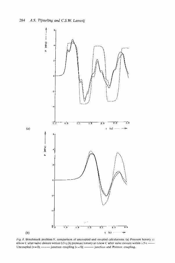
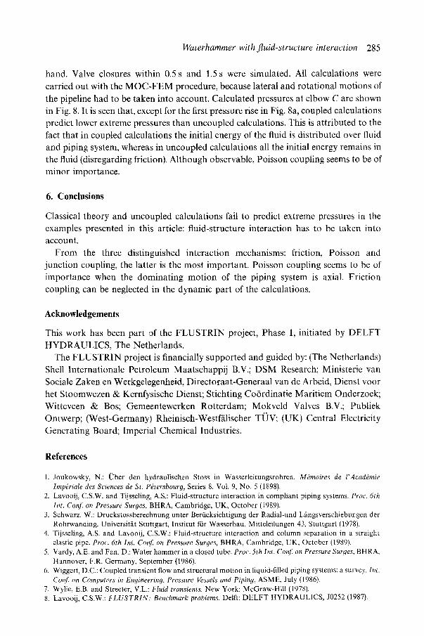
Fig. 8. Benchmark problem F, comparison of uncoupled and coupled calculations. (a) Pressure history at elbow C after valve closure within 0.5 s; (b) pressure history at elbow C after vatve closure within 1.5 s. - . . . . . Uncoupled (v=O); - - - junct ion coupling (v-O); junct ion and Poisson coupling.

W a t e r h a m m e r w i t h f l u i d - s t r u c t u r e i n t e rac t i on 285

hand. Valve closures within 0.5 s and 1.5 s were simulated. All calculations were

carried out with the M O C - F E M procedure, because lateral and rotational motions of

the pipeline had to be taken into account. Calculated pressures at elbow C are shown in Fig. 8. It is seen that, except for the first pressure rise in Fig. 8a, coupled calculations predict lower extreme pressures than uncoupled calculations. This is attributed to the fact that in coupled calculations the initial energy of the fluid is distributed over fluid and piping system, whereas in uncoupled calculations all the initial energy remains in

the fluid (disregarding friction). Although observable, Poisson coupling seems to be of minor importance.

6. Conclusions

Classical theory and uncoupled calculations fail to predict extreme pressures in the

examples presented in this article: fluid-structure interaction has to be taken into account,

From the three distinguished interaction mechanisms: friction, Poisson and junction coupling, the latter is the most important. Poisson coupling seems to be of importance when the dominating motion of the piping system is axial. Friction

coupling can be neglected in the dynamic part of the calculations.

Acknowledgements

This work has been part of the F L U S T R I N project, Phase 1, initiated by D E L F T

HYDRAULICS, The Netherlands. The F L U S T R I N project is financially supported and guided by: (The Netherlands)

Shell Internationale Petroleum Maatschappij B.V.; DSM Research; Ministerie van Sociale Zaken en Werkgelegenheid, Directoraat-Generaal van de Arbeid, Dienst voor het Stoomwezen & Kernfysische Dienst; Stichting Co6rdinatie Maritiem Onderzoek;

Witteveen & Bos; Gemeentewerken Rotterdam; Mokveld Valves B.V.; Publiek Ontwerp; (West-Germany) Rheinisch-Westf/ilischer Tf]V; (UK) Central Electricity

Generating Board; Imperial Chemical Industries.

References

1. Joukowsky, N.: Uber den hydraulischen Stoss in Wasserleitungsrohren. M~moires de l'Acadkmie Imp~riale des Sciences de St. Pktersbourg, Series 8, Vol. 9, No. 5 (1898).

2. Lavooij, C.S.W. and Tijsseling, A.S.: Fluid-structure interaction in compliant piping systems. Proc. 6th Int. Conf. on Pressure Surges, BHRA, Cambridge, UK, October (1989).

3. Schwarz, W.: Druckstossberechnung unter Beriicksichtigung der Radial-und L/ingsverschiebungen der Rohrwanding. Universit~it Stuttgart, Institut fiir Wasserbau, Mitteleilungen 43, Stuttgart (1978).

4. Tijsseling, A.S. and Lavooij, C.S.W.: Fluid-structure interaction and column separation in a straight elastic pipe. Proc. 6th Int. Conf. on Pressure Surges, BHRA, Cambridge, UK, October (1989).

5. Vardy, A.E. and Fan, D.: Water hammer in a closed tube. Proc. 5th Int. Conf. on Pressure Surges, BHRA, Hannover, F.R. Germany, September (1986).

6. Wiggert, D.C.: Coupled transient flow and structural motion in liquid-filled piping systems: a survey. Int. Conj'. on Computers in Engineering, Pressure Vessels and Pipiny, ASME, July (1986).

7. Wylie, E.B. and Streeter, V.L.: Fluid transients. New York: McGraw-Hill (1978). 8. Lavooij, C.S.W.: F L U S T R I N : Benchmark problems. Delft: DELFT HYDRAULICS, J0252 (1987).