Embed Size (px)
Citation preview
WATER AND FARM EFFICIENCY: INSIGHTS FROM THE FRONTIER LITERATURE
Authors: Boris E. Bravo-‐Ureta: Agricultural and Resource Economics University of Connecticut and Agricultural and Economics Universidad de Talca, Chile, corresponding author [email protected] Roberto Jara-‐Rojas: Agricultural Economics Universidad de Talca, Chile [email protected] Michée A. Lachaud: Agricultural and Resource Economics University of Connecticut [email protected] Víctor H. Moreira L. Agricultural Economist, Universidad Austral de Chile, Chile [email protected] Susanne M. Scheierling: Sr. Irrigation Water Economist, Water Global Practice, The World Bank, Washington D.C. [email protected]
Selected Paper prepared for presentation at the 2015 Agricultural & Applied Economics Association and Western Agricultural Economics Association Annual Meeting, San Francisco, CA,
July 26-‐28
Copyright 2015 by [authors]. All rights reserved. Readers may make verbatim copies of this document for non-‐commercial purposes by any means, provided that this copyright notice
appears on all such copies.
1
WATER AND FARM EFFICIENCY: INSIGHTS FROM THE FRONTIER LITERATURE*
Boris E. Bravo-‐Ureta1, Roberto Jara-‐Rojas2, Michée A. Lachaud3, Víctor H. Moreira L.4, Susanne M. Scheierling5
Abstract This paper presents an overview of a recently completed meta-‐analysis of the frontier function literature focusing on the technical efficiency (TE) component of water productivity in agriculture. A descriptive analysis is first performed for a comprehensive meta-‐dataset that includes 409 farm level TE studies, published between 1981 and mid-‐2014. Of this total of 409, 94 are water studies—defined here as those that explicitly include irrigation and/or precipitation in the analysis. Some studies report several mean TEs, resulting in 904 observations or cases. The Average of the Mean Technical Efficiencies (AMTE) reported for all studies is 74.3%, with 74.5% for non-‐water studies vs. 73.4% for water studies. The analysis reveals considerable heterogeneity in the methods used and with regard to how water is defined and treated. Some studies include volumetric measures of irrigation water and combine this with a robust methodology that provides measures of irrigation water use efficiency (IWUE). The latter quantifies the amount of water that could be saved on-‐farm while holding output, other inputs and the technology constant. This methodology, particularly when implemented along with a parametric model, can provide valuable information not only on IWUE but also on other key economic parameters for irrigation water (e.g., shadow values, production elasticities). Despite the importance of water in farming and the continued vibrancy of the productivity literature, it is surprising how little analytical work has been carried out in this critical field. Keywords: Irrigation Water Use; Technical Efficiency; Agriculture; Meta-‐Analysis. JEL Classification: Q25, Q12, D24.
•• This study was partially funded by the Water Partnership Program (WPP), a multi-‐donor trust fund at the World Bank.
1Agricultural Economist, University of Connecticut and Universidad de Talca, Chile corresponding author [email protected]
2 Agricultural Economist, Universidad de Talca, Chile [email protected] 3 Agricultural Economist, University of Connecticut, USA [email protected] 4Agricultural Economist, Universidad Austral de Chile, Chile [email protected] 5 Sr. Irrigation Water Economist, Water Global Practice, The World Bank, Washington D.C. [email protected]

2
WATER AND FARM EFFICIENCY: INSIGHTS FROM THE FRONTIER LITERATURE 1. INTRODUCTION Irrigation water worldwide accounts for approximately 70% of all freshwater withdrawals, which generate low returns relative to other water using sectors. It is expected that increasing water scarcity will put pressure on farming to reduce consumption so that water can be diverted elsewhere. Therefore, it becomes critical to improve the productivity and efficiency of water use in agriculture. However, the literature that deals with the role of water on farm productivity provides limited insights on actions that could be taken to increase agricultural production while using water in a way that avoids adding to the scarcity of the resource (Scheierling et al. 2014). The objective of this paper is to provide an overview of the frontier function literature and then focus on water productivity and Technical Efficiency (TE) studies, building on previous meta-‐analyses work by Bravo Ureta et al. (2007) and Moreira and Bravo-‐Ureta (2009). This paper, which is extracted from a more detailed study, contributes to the existing frontier function literature by providing an up to date systematic and comprehensive analysis of the effects that different methodologies and study-‐specific attributes have on mean TE scores. Moreover, we focus on water studies, defined here as those that explicitly include irrigation and/or precipitation in the analysis of TE. This detailed focus on water appears to be the first of its kind. A comprehensive literature search has been conducted yielding a total of 425 TE studies, 409 or which reported TE at the farm level, our main focus. The total number of studies with a focus on water is 110. The remainder of this paper is structured as follows. Section 2 contains an overview discussion of the alternative methodologies used in frontier analysis. Section 3 presents the approach followed to generate the data used in the meta-‐analysis, and presents a descriptive analysis of the data. The paper continues with a discussion of the water papers in Section 4, and Section 5 provides some concluding remarks. 2. OVERVIEW OF FRONTIER METHODOLOGIES Although preceded a few years by Debreu (1951) and Koopmans (1951), the 1957 seminal paper by Farrell is widely credited as the intellectual impetus that has propelled frontier function research (Fried, Lovell and Schmidt 2008; Greene 2008). Farrell relied on the efficient unit isoquant to define and measure TE, allocative efficiency (AE), and economic efficiency (EE). The focus in this study is farm level TE, so this methodological summary favors this particular efficiency concept as opposed to a number of other related notions. Our intention is not to provide an exhaustive review but rather to point out some of the key features that appear in the studies included in our meta-‐analysis. For clarity it is important at the outset to differentiate between Technological Change (TC) and TE. TC measures shifts of the production frontier stemming from the fruit of innovation (Färe, Grosskopf and Margaritis 2008). By contrast, TE has to do with the distance a firm operates relative to its frontier and such distance can be measured with input or an output orientation. In the simple single input production frontier case, the output oriented

3
approach, which is most commonly used in applied work, TE is given by the ratio between the observed and the maximum (frontier) level of output that can be produced given a quantity of input and the technology. By contrast, the input orientated approach is given by the ratio of the quantity of input needed to produce a given level of output if the farm operates on the frontier relative to the input actually used. Therefore, TE, whether input or output oriented, is an index that ranges between 0% and 100% and can be interpreted as a proxy measure for managerial effort or performance (Martin and Page 1983; Triebs and Kumbhakar 2013). Analogous measures can be defined for the multiple input-‐multiple output technologies (Coelli et al. 2005). Frontier function methods have become widely used in applied production economics given their consistency with the neo-‐classical notion of maximization or minimization imbedded in the definitions of production, revenue, profit and cost functions. The popularity of frontier methods is substantiated by the abundance of methodological and empirical frontier studies over the last three decades. Methodological reviews of the panoply of models that have been developed can be found in Førsund, Lovell and Schmidt (1980); Schmidt (1985-‐86); Bauer (1990); Seiford and Thrall (1990); Kumbhakar and Lovell (2000); Fried, Lovell and Schmidt (2008); Greene (2008); and Thanassoulis, Portela and Despić (2008), among others. The popularity of applied frontier studies in agriculture is documented in several reviews and meta-‐analyses including Battese (1992), Bravo-‐Ureta and Pinheiro (1993), Thiam, Bravo-‐Ureta and Rivas (2001), Gorton and Davidova (2004), Bravo-‐Ureta et al. (2007), Moreira and Bravo-‐Ureta (2009), Darku, Malla and Tran (2013), Minviel and Latruffe (2013), and Ogundari (2014). The frontier methodology is commonly divided into parametric and non-‐parametric methods. Parametric methods require the specification of a functional form for the technology (e.g., Cobb-‐Douglas, Translog) whereas non-‐parametric models do not have such requirement and this constitutes a major advantage of the latter. Parametric models can be subdivided into deterministic and stochastic frontier analysis (SFA) where the former assumes that any deviations from the frontier stem from inefficiency, while the stochastic approach incorporates statistical noise (Coelli et al. 2005). Hence, a key limitation of deterministic frontiers is that measurement errors, as well as other sources of random variation are captured as inefficiency and this means that outliers have a distorting effect on TE scores (Fried, Lovell and Schmidt, 2008). The stochastic frontier model, developed separately but around the same time by Aigner, Lovell and Schmidt (1977) and Meeusen and van den Broeck (1977), copes with outliers through a composed error structure with a two-‐sided symmetric term and a one-‐sided component. The two-‐sided error captures random shocks outside the control of the firm whereas the one-‐sided component takes care of inefficiency. Non-‐parametric frontiers trace their origin directly to Farrell (1957); however, it took almost 20 years for non-‐parametric frontiers to get a firm footing in the literature and such is due to the seminal contribution by Charnes, Cooper and Rhodes (1978). As already noted, the main feature of non-‐parametric frontiers is that they do not require the specification of a functional form while a major drawback is that these methods are deterministic and thus sensitive to extreme observations. In addition, the TE scores generated by non-‐parametric

4
methods can be sensitive to the number of observations in the data and to the dimensionality of the frontier. Non-‐parametric measures of efficiency are obtained using mathematical programming techniques widely known as Data Envelopment Analysis or DEA (Thanassoulis, Portela and Despić 2008). This area of the frontier literature gained major popularity early on in management science and operations research but now is also firmly established in economics including agricultural economics (Fried, Lovell and Schmidt 2008). Frontier studies can also be separated into primal and dual. The primal approach has been more common in frontier estimation since it does not require price data, often difficult to get at the firm/farm level, nor does it rely on maintained hypothesis regarding behavior such as cost minimization or profit maximization (Coelli et al. 2005). The validity of dual models has been questioned, particularly when profit maximization is the maintained hypothesis in the context of developing country agriculture (e.g., Junankar 1980). An important advantage that non-‐parametric models enjoyed for a number of years is their ability to easily accommodate multi-‐input multi-‐output technologies within a primal specification. By contrast, to accommodate such technologies, parametric models had to appeal initially to dual cost or profit frontiers, which presented data challenges as well as the need to make stringent behavioral assumptions (e.g., Ali and Flinn 1987; Bailey et al. 1989). More recently, developments in the parametric stochastic literature have enabled the estimation multi-‐input multi-‐output models by means of input and output distance functions. The main advantage of using a distance function is that price information is not needed and these models can be estimated without assuming input-‐output separability (Coelli 2005). A further extension is the directional distance function, which is a generalization of the input and output distance functions. The directional distance specification simultaneously allows for the expansion of outputs and the reduction of inputs toward all points that are on the frontier and dominate the observation being assessed (Färe, Grosskopf and Margaritis 2008). Directional distance functions have also been used to incorporate bad outputs and examine the tradeoff between good and bad outputs (e.g., Njuki and Bravo-‐Ureta 2015 and papers cited therein). Frontier function analyses can also be characterized in terms of the type of data used, as cross-‐section or panel. Frontier estimation with panel data has made considerable progress in both the non-‐parametric and the parametric worlds and this is an appealing feature because it can significantly enhance the analysis particularly in decomposing total factor productivity change in terms of TC, TE change (TEC) and scale efficiency change (SEC) (Kumbhakar and Lovell 2000; Fried, Lovell and Schmidt 2008). In the stochastic approach, the recent work by Greene (2005a; 2005b) has opened up useful options to account for time invariant firm heterogeneity in addition to time variant TE. Very recently, several authors have presented and applied models that decompose (overall) efficiency into a persistent (long-‐run) and a transient (short run) component while also capturing unobserved time invariant heterogeneity (Colombi et al. 2014; Filippini and Greene 2014; Kumbhakar, Lien and Hardaker 2014; Tsionas and Kumbhakar 2014; Lachaud, Bravo-‐Ureta and Ludena 2014). Panel data methodologies clearly offer an interesting path forward but the challenge is to develop the necessary data sets to take full advantage of the emerging methods.

5
Another strand on the frontier literature has to do with efforts geared at explaining the variability of TE in terms of exogenous factors that typically include socioeconomic and environmental variables. The original approach is the so called two-‐step model where TE is estimated in the first step, using any of the models we have discussed, without accounting for exogenous and environmental factors and then in the second-‐step TE is regressed on such factors (Greene 2008; Bravo-‐Ureta and Pinheiro 1993). Examination of the validity of the two-‐step procedure indicates that this approach leads to biased or invalid results in both parametric and non-‐parametric models (Wang and Schmidt 2002; Simar and Wilson 2007). Taking a forceful position on this matter, Fried, Lovell and Schmidt (2008) state: “We hope to see no more two-‐stage SFA models” (p. 39). These objections of the validity of two-‐step models have motivated the development of one-‐step procedures in the stochastic frontier literature, where the most widely applied model is the one presented by Battese and Coelli (1995). Progress has also been made in the explanation of TE in the non-‐parametric literature using bootstrapping techniques. Simar and Wilson (2007; 2008) argue that the results of many studies that have estimated second-‐step regressions to explain the variation in TE scores, derived from DEA models, have produced invalid results. The first problem they pinpoint is that a large volume of these studies do not describe the associated data generating process (DGP) “that would make a second-‐stage regression sensible” (Simar and Wilson 2008, p 501). A second and “more serious problem in all of the two stage studies” found by Simar and Wilson (2007) “arises from the fact DEA efficiency estimates are serially correlated” (p. 33). The latter invalidates any inferences regarding the parameters of the second-‐step regression. These authors then present a DGP that affords the foundation for the second-‐step regression of TE scores from DEA models. The authors also present a truncated regression model along with a double bootstrap approach and argue that this framework makes it possible to obtain unbiased TE scores (first bootstrap) and valid estimates of confidence intervals for the coefficients of the second-‐step regression (second bootstrap) while increasing statistical efficiency in the estimation. Examples of applications of this procedure in agriculture include Latruffe, Davidova and Balcombe (2008), Balcombe et al. (2008), and Keramidou and Mimis (2011). An additional and emerging strand of the literature we want to mention concerns recent efforts in stochastic frontier models to correct for selectivity bias (Kumbhakar, Tsionas and Sipiläinen 2009; Lai, Polachek and Wang 2009; Greene 2010). Bravo-‐Ureta, Greene and Solís (2012) have combined the Greene (2010) model with Propensity Score Matching (PSM) to account for biases from observable and unobservable variables in order to decompose the impact of development projects into output growth (i.e., upwards shifts in the production frontier due to TC) and management improvements (i.e., narrowing the gap from the frontier) when only cross sectional data are available (Bravo-‐Ureta 2014). The model is applied to data generated from the MARENA Project in Honduras. Additional applications of the Bravo-‐Ureta, Greene and Solís (2012) model include the work by González-‐Flores et al. (2014) for a sample of small-‐scale potato farmers from Ecuador and by Villano et al. (2014) who investigate the impact of adopting certified seed varieties on the productivity of rice farmers in the Philippines. Another area that is receiving attention in the recent literature concerns the possible

6
endogeneity of inputs in stochastic frontiers. Zellner, Kmenta and Drèze (1966) provided what has become the classical justification for valid econometric estimates of production functions. These authors assumed that firms maximize the mathematical expectation of profits rather than deterministic profits. More recently, several authors such as Tran and Tsionas (2013), and Shee and Stefanou (2014) have proposed alternative approaches to tackle endogeneity in stochastic frontier models building on previous work by Olley and Pakes (1996), Levinsohn and Petrin (2003), and Kutlu (2010), among others. Is useful to underscore that major methodological advances have been made in both parametric (econometric) and non-‐parametric (programming) frontiers. Paraphrasing from Fried, Lovell and Schmidt (2008), SFA and DEA have important similarities as well as differences. Both approaches are rigorous analytical tools to measure efficiency relative to a frontier. “At the risk of oversimplification, the differences between the two approaches boil down to two essential features: [1] The econometric approach is stochastic. This enables it to attempt to distinguish the effects of noise from those of inefficiency, thereby providing the basis for statistical inference. [2] The programming approach is nonparametric. This enables it to avoid confounding the effects of misspecification of the functional form (of both technology and inefficiency) with those of inefficiency” (p. 32-‐33). Despite the ‘conciliatory’ remarks in the preceding paragraph, in a recent paper O’Donnell (2014) argues that the core assumptions on which the DEA machinery stands “… are rarely, if ever true (e.g., output, input and environmental variables are almost always measured with error, if not unobserved). It follows that most, if not all, DEA estimators are inconsistent” (p. 22). O’Donnell goes on to quote Simar and Wilson (2000) who wrote: “Consistency is an essential property of any estimator [p. 56].…. If the data contains noise, DEA … estimators will be inconsistent, and there seems little choice but to rely on SFA [p. 76].” One is left with the distinct impression that the SFA-‐DEA controversy will go on for a few more rounds. 3. GENERATION OF THE DATASET AND DESCRIPTIVE ANALYSIS A key aspect in a meta-‐analysis is to conduct a thorough and systematic review of the literature to develop the list of papers to be included in the investigation. We performed a comprehensive search of the literature using the following databases: EBSCOhost, Econlit, Academic Search Premier, Agricola, Scopus and ISI Web of Knowledge which includes Agris International, Science Direct and Social Science Citation Index. An additional search was done for specific journals that overtime have published a good number of applied TE studies and/or are major outlets of agricultural economics work. The journals included are the American Journal of Agricultural Economics, the Journal of Agricultural Economics, Agricultural Economics, the European Review of Agricultural Economics, the Australian Review of Agricultural and Resources Economics, the Canadian Journal of Agricultural Economics, the Journal of Productivity Analysis, Empirical Economics, the European Journal of Operations Research and Applied Economics.
A complementary search was conducted for water related TE papers using the following key words: Irrigation, Technical Efficiency, Farming, Agriculture, Productivity and Frontier, water, water use, groundwater, water flows, return flows, water quality, and leaching which

7
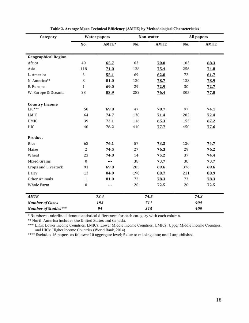
were combined in different ways to expand the search. It is important to emphasize that the two critical and necessary key words in all searches were Technical Efficiency and Agriculture. In other words, we keep only the papers related to TE and Agriculture. The combined searches, limited to papers written in English, yielded a total of 409 farm level papers that contain all the data required for our analysis.1 Descriptive Analysis As indicated, the total number of studies with a water focus is 110. Of this 110, 16 are only partially included in the study due to the following reasons: missing data [5]; use of aggregate data [10], considering that our main focus is on farm level studies; and [1] is in the grey literature and thus outside the criteria used for selecting the studies. The latter study, however, is incorporated in the longer version of this paper because it brings a novel dimension to the discussion. In sum, for the primary analysis presented here, we have a total of 409 farm-‐level studies, 315 without a water focus and 94 with. The key variable in our analyses is the mean technical efficiency (MTE) reported in each paper. Some papers present more than one MTE due to the use of alternative methods, so the total number of MTEs, or cases, from the 409 studies is 904, of which 193 come from the water studies. Table 1 shows that of the 904 total cases, 623 come from parametric and 281 from non-‐parametric models; in addition, 552 observations come from stochastic and 352 from deterministic frontiers. The AMTE for all papers is 74.3%, which is slightly lower than the 76.6% reported by Bravo-‐Ureta et al. (2007). For the 193 water cases, Table 1 indicates that 120 come from parametric and 73 from non-‐parametric models, and 120 are from stochastic and 73 from deterministic frontiers. The AMTE for all water papers is 73.4%, which is slightly lower that the value of 74.5% for non-‐water papers but this difference is not statistically significant. Table 1 also reports statistical tests for the null hypothesis that AMTE for each category is the same and, overall, we observe only a few differences. For the non-‐water papers, there is a significant difference between the stochastic and deterministic approaches (75.4% vs. 73.3%, respectively). Another significant difference is for the data structure category in both the non-‐water and all cases, where panel data is higher than cross sectional (77.7% vs. 72.6% for non-‐water, and 77.3% vs. 73.5% for water). The last difference is for functional form where TL is higher than CD (78.3% vs. 72.0% for non-‐water, and 77.3% vs. 72.4% for water). Looking at the highest AMTE for each of the three groups, we see that the top value for the water papers is for panel data (76.3%), while the TL is at the top for non-‐water (78.3%). For all papers combined, the panel data and TL groups exhibit the highest AMTE, both at 77.3%. Table 2 contains a summary of AMTE for various groupings according to geographical region, income category and product type. The following six geographical regions are included: Africa, Asia, Latin America, North America, Eastern Europe, and Western Europe and Oceania. In terms of country income, we use the following four categories based on the World Bank (2014): LICs (Lower Income Countries); LMICs (Lower Middle Income Countries); UMICs (Upper Middle Income Countries); and HICs (Higher Income Countries). 1 The list of all 409 papers, including those reviewed in Section 4, is available from the authors upon request.

8
The product groups are as follows: Rice; Maize; Wheat; Mixed Grains; Crops and Livestock; Dairy; Other Animals; and Whole Farm. As is the case with Table 1, we note only a few significant AMTE differences. The data shows that AMTE for water papers is higher in W. Europe and Oceania (83.9%) and lowest for Latin America (55.1%). For the country income category, there is no difference for the water studies, but the non-‐water studies show the highest values for LIC (78.7%) and HIC (77.7%) and the same pattern for all studies (74.1% LIC and 77.6% HIC) and the lowest for UMIC (65.3% for non water and 67.2% for all). The last point we want to make in this comparison is that Dairy farming exhibits the highest AMTE across products for all three study groups -‐-‐ 84% water, 80.7% non-‐water and 80.9% all-‐-‐ and is statistically significant in the last two. Taking a broader look at the data in Table 2 we see that the lowest AMTE values for both water and non-‐water papers and thus for all papers combined is for Latin America (55.1%, 62.0% and 61.7%) and Africa (65.7%, 70.0% and 68.3%). By contrast, North America (81.0% water; 78.7% non-‐water; 78.9% all), and W. Europe and Oceania (83.9% water; 76.4% non-‐water; 77.0% all) have the highest AMTEs. By comparison, Bravo-‐Ureta et al. (2007) find that the lowest AMTE for all cases analyzed by them is for Eastern Europe (70.0%) followed by Africa (73.7%) while the highest is for W. Europe and Oceania (82.0%) followed by Latin America (77.9%). Aggregating the countries by income leads to a fairly irregular pattern although the HICs have the highest AMTE for all papers at 77.6% and the UMICs the lowest at 67.2%. This latter pattern is consistent with Bravo-‐Ureta et al. who report an AMTE of 78.8% for HICs (their highest) and 68.3% for UMICs (their lowest). Turning to the Product grouping we see that the lowest AMTE for all three types of papers in Table 2 is for Crops and Livestock (69.8% water; 69.6% non-‐water; 69.6% all). By contrast the highest AMTE is uniformly for dairy papers at 84.0% for water, 80.7% for non-‐water and 80.9% for all papers. It is interesting to note that this is very close to the results of Bravo-‐Ureta et al. (2007) who reported an AMTE for dairy and cattle of 80.6% which is the second highest average in their paper following Other Animals at 84.5% but the latter only has six observations. In sum, this section presented a descriptive analysis of 409 farm level studies, 315 non-‐water and 94 with some type of water focus. The respective AMTE is 74.3%, 74.5% and 73.4%. The AMTE across methodological attributes tend to be quite similar for the two groups of studies but several significant differences are observed when comparisons are made across geographical regions, income levels, and type of product. Some comparisons are made with the previous comprehensive meta-‐analysis by Bravo-‐Ureta et al. (2007).
4. ANALYSIS OF WATER STUDIES Now we classify all 110 water studies, which includes 94 at the farm level plus 16 other studies, 10 of which use aggregate data, five do not report TE and one is a working paper. We have classified these 110 papers into five groups, A through E, and in some cases into additional subgroups. The studies in Groups A through D use farm level data while those in Group E use aggregate data. The five groups (A-‐E) are:
9
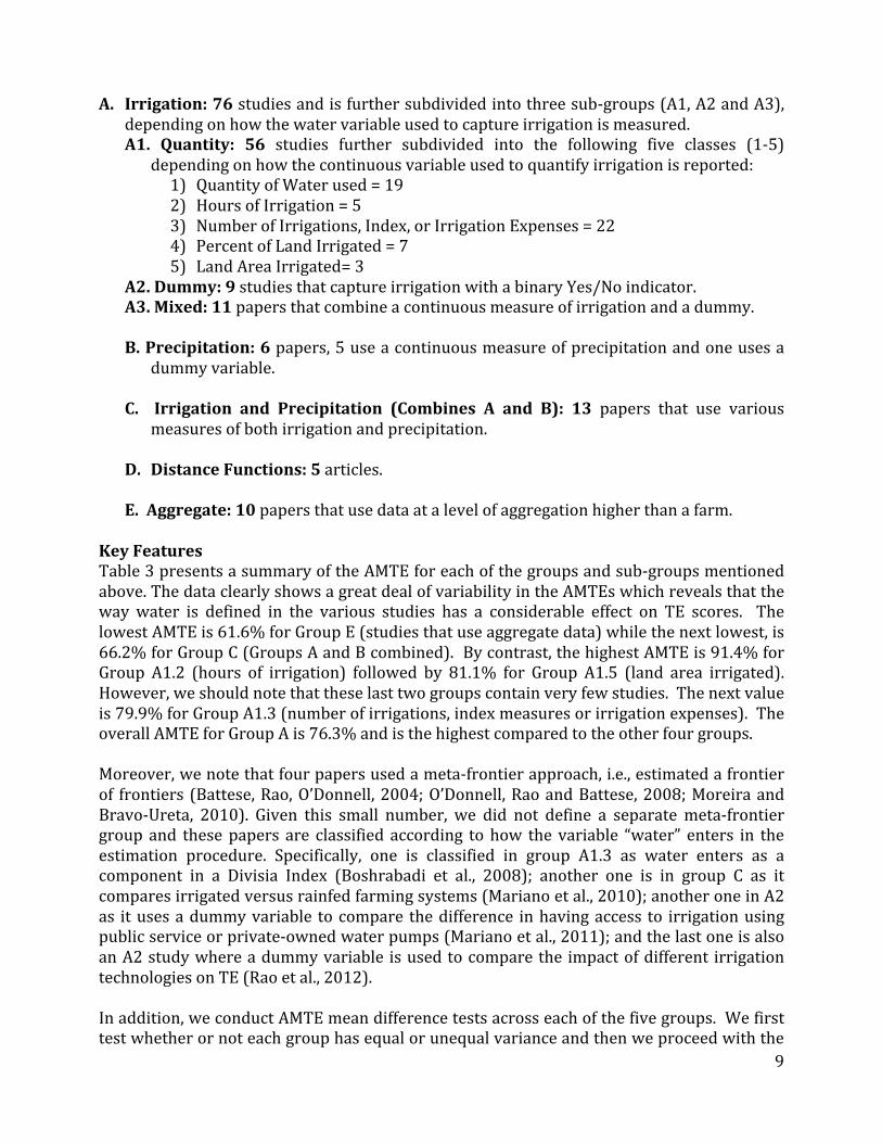
A. Irrigation: 76 studies and is further subdivided into three sub-‐groups (A1, A2 and A3), depending on how the water variable used to capture irrigation is measured. A1. Quantity: 56 studies further subdivided into the following five classes (1-‐5)
depending on how the continuous variable used to quantify irrigation is reported: 1) Quantity of Water used = 19 2) Hours of Irrigation = 5 3) Number of Irrigations, Index, or Irrigation Expenses = 22 4) Percent of Land Irrigated = 7 5) Land Area Irrigated= 3
A2. Dummy: 9 studies that capture irrigation with a binary Yes/No indicator. A3. Mixed: 11 papers that combine a continuous measure of irrigation and a dummy.
B. Precipitation: 6 papers, 5 use a continuous measure of precipitation and one uses a
dummy variable.
C. Irrigation and Precipitation (Combines A and B): 13 papers that use various measures of both irrigation and precipitation.
D. Distance Functions: 5 articles. E. Aggregate: 10 papers that use data at a level of aggregation higher than a farm.
Key Features Table 3 presents a summary of the AMTE for each of the groups and sub-‐groups mentioned above. The data clearly shows a great deal of variability in the AMTEs which reveals that the way water is defined in the various studies has a considerable effect on TE scores. The lowest AMTE is 61.6% for Group E (studies that use aggregate data) while the next lowest, is 66.2% for Group C (Groups A and B combined). By contrast, the highest AMTE is 91.4% for Group A1.2 (hours of irrigation) followed by 81.1% for Group A1.5 (land area irrigated). However, we should note that these last two groups contain very few studies. The next value is 79.9% for Group A1.3 (number of irrigations, index measures or irrigation expenses). The overall AMTE for Group A is 76.3% and is the highest compared to the other four groups. Moreover, we note that four papers used a meta-‐frontier approach, i.e., estimated a frontier of frontiers (Battese, Rao, O’Donnell, 2004; O’Donnell, Rao and Battese, 2008; Moreira and Bravo-‐Ureta, 2010). Given this small number, we did not define a separate meta-‐frontier group and these papers are classified according to how the variable “water” enters in the estimation procedure. Specifically, one is classified in group A1.3 as water enters as a component in a Divisia Index (Boshrabadi et al., 2008); another one is in group C as it compares irrigated versus rainfed farming systems (Mariano et al., 2010); another one in A2 as it uses a dummy variable to compare the difference in having access to irrigation using public service or private-‐owned water pumps (Mariano et al., 2011); and the last one is also an A2 study where a dummy variable is used to compare the impact of different irrigation technologies on TE (Rao et al., 2012). In addition, we conduct AMTE mean difference tests across each of the five groups. We first test whether or not each group has equal or unequal variance and then we proceed with the

10
testing of mean differences. The findings show that there is no statistically significant difference in AMTE across Groups except for Group A and C and Group A and E. The AMTEs across the other groups are statistically the same. Is important to underscore that TE provides a measure of the gap between what is produced and what could be produced given inputs, the environment, and the technology, but it does not give any insight about water use efficiency per se. Irrigation Water Use Efficiency (IWUE) Studies Here we provide a more detailed analysis of 11 studies that, in addition to providing a conventional analysis of TE, examine irrigation water use efficiency (IWUE). The general unifying theme in these studies is the use of a methodology introduced by Reinhardt et al. (1999) that makes it possible to derive non-‐radial measures of efficiency for an input of interest, which in our case is irrigation water. Reinhardt et al. (2002) extended this methodology in order to estimate a second step model to explain IWUE in a manner that is compatible with econometric assumptions. Another analysis that can be done, following Akridge (1989), is to evaluate the feasible cost savings that could be achieved by managing water more efficiently. This has been termed in this literature Irrigation Water Technical Cost Efficiency or IWTCE. This term can be defined as the cost savings that are possible by holding irrigation water use at its technically efficient level while other inputs are held constant at their observed levels. To illustrate this methodology, we cast our discussion assuming a deterministic parametric model; however, it should be understood that similar analyses can be performed using a stochastic production frontier (e.g., Karagiannis, Tzouvelekas and Xepapadeas, 2003) as well as a sub-‐vector DEA approach (e.g., Lilienfeld and Asmild, 2007). We highlight this methodology because it appears as a promising area for further empirical work and methodological refinements. Figure 1 presents a graphical illustration of an output measure of efficiency assuming for simplicity that water is the only variable input. A firm (point C) that uses IW1 to produce Y0 units of output operates considerably below the maximum level of output Ym that could be attained by operating on the frontier (point B). Thus, the level of TE for this firm is equal to the ratio OY0/OYM. Alternatively, we could compare the amount of water actually used with the amount that would be used by operating on the frontier to attain Y0 output. Based on the graph, the input oriented measure of TE is given by OIW0/OIW1, for output Y0 while holding other inputs and the level of technology constant. In Figure 2 we can observe that a hypothetical inefficient firm operates at point A using OW1 units of water and OX1 units of all other inputs to produce Y0 output. The input oriented measure of TE in this case is OB/OA. Again, if we focus on the input savings side we can observe that a non-‐radial measure of efficiency can be expressed as X1C/X1A or alternatively as OW2/OW1. These measures, which are equivalent to each other, represent the amount of water that could be reduced if the firm was to move to the frontier holding X constant at X1 and still produce Y0. This measure has become known in the literature as Irrigation Water Efficiency (IWE), Irrigation Water Technical Efficiency (IWTE) or Irrigation Water Use Efficiency (IWUE). Here we adopt the term IWUE. Finally, it is useful to note the difference between IWUE and the water savings that is achieved, OW1-‐OW3, by the radial contraction of both inputs to get to the technically efficient point B. OW1-‐OW3 is an input oriented measure of TE.

11
Before turning to a review of the 11 IWUE papers, we present in Table 4, without much discussion, key features of 48 Non-‐IWUE studies that report a number of informative farm output responses to water, including partial elasticities of production with respect to: volume of irrigated water applied; irrigation expenditures; hours a plot is irrigated; number of times a plot is irrigated during a particular season; and the amount or percent of irrigated land. As the data in Table 4 shows, these response indicators clearly show that irrigation has a positive and significant effect on output. Now we highlight the key aspects of the 11 IWUE studies, which are shown in Table 5. First, AMTE is 70.4% ranging from 61.5% to 81%. Three papers show Irrigation Water Technical Cost Efficiency (ITCE) with an average of 84.4%. All 11 papers report IWUE with an average of 47.2% ranging from 15.7% to 69.9%. We now present a few remarks for each of the 11 IWUE papers. We start with Dhehibi, Lachaal and Elloumi (2007) (A1. 1-‐6) who used data for a sample of 144 citrus farms from the area of Nabeul in Tunisia. They used a Translog functional form along with a Battese and Coelli (1995) model to explain the variation in TE and the Reinhartd et al. (2002) two-‐stage approach to investigate the variables that influence IWUE. Irrigation water exhibited the largest partial elasticity of production equal to 0.298 and returns to scale equal to 1.106 (at the mean of the data). The authors report Mean IWUE and output oriented TE at 53.0% and 67.7%, respectively while mean IWTCE is 70.8. The value for IWUE suggests that the average farmer could produce the same level of output with 47% less water. This study also reports that both TE and IWUE are associated with farmer’s age, education level, agricultural training, farm size, share of productive trees and water availability. Frija et al., (2009) (A1.1-‐9) examined data collected in 2005 for a sample of 47 small-‐scale greenhouse producers of (primarily) tomatoes, melons and peppers located in the region of Teboulba in east-‐central Tunisia. The authors used the DEA sub-‐vector efficiency methodology to calculate IWUE and a second stage tobit model to analyze the association between TE and IWUE with various explanatory variables. The analysis showed that farmers in the samples in the farmer are overall producing at the right scale. Results obtained assuming constant returns to scale reveal an average TE equal to 67.3% while average IWUE is reported at 42%. The authors conclude that providing framers with training in greenhouse management, investments in water saving technologies and fertigation techniques (i.e., the mixing of irrigation water with fertilizers can be expected to enhance IWUE. In contrast, the authors find that the proportion of total farmland assigned to greenhouses had a significant negative association with IWUE. Wang (2010), which is paper A1.1-‐18, uses DEA along with data collected for the 2006 crop year from a sample of 432 wheat producers located in 11 villages in Northwestern China to examine TE and IWUE. Water measured in m3, along with several other inputs is introduced into the model. An average TE of 61.5% is reported using an output oriented measure and a CRS model. By contrasts the average input-‐oriented IWUE is 30.7%. The author also calculated the more traditional single factor efficiency and found that on average 0.61 kg of wheat is produced per m3 of water used. The author then applied a second step Tobit regression model to examine the determinants of IWUE. The results show that additional experience and financial strength are associated with higher irrigation water efficiency,

12
while an inverted u-‐shaped association between IWUE and water flow is reported. The author also argues that a gradual introduction of water prices would likely lead to a more efficient use of water. Another paper using data from Tunisia is by Mahdhi, Sghaier and Bachta (2011) (A1.1-‐12) who used data collected between April 2005 and August 2009 for a sample of 100 small-‐scale private irrigated farms in the region of Zeuss-‐ Koutine in south-‐eastern Tunisia. This study evaluates TE and IWUE and, under variable returns to scale, the average TE for the sample was 80.3% while average IWUE was 60%. Yet another study for Tunisia using the DEA sub-‐vector efficiency methodology is by Chemak (2012) (A1.1-‐4) who used 2007, 2008 and 2009 data for 47 farms that grew olive trees, cereal crops, forage crops and horticulture crops. The results showed an average TE, IWUE and scale equal to 81%, 68% and 88%. Njiraini and Guthiga (2013), paper A1-‐14, focus on TE and IWUE, while also examining the variables associated with the latter. A cross sectional data set, collected in March-‐April 2010, including 201 small scale irrigation farmers located in the lake Naivasha basin along with a variable returns to scale DEA model are used to estimate input oriented TE. The model incorporates a single output in value terms and several inputs including the quantity of water used for irrigation measured in m3. Once TE is calculated the authors implement a sub-‐vector efficiency analysis to calculate IWUE while holding output and all other inputs constant. The results show an average TE equal to 63.3% and an average IWUE equal to 31.9% with a Pearson correlation coefficient for these two efficiency vectors of 0.68. They then proceed with a second step Tobit model to examine the variables that might be associated with IWUE. The Tobit model includes various socioeconomic variables, crop choice as an indicator of profitability, a land fragmentation index, a dummy variable to capture membership in a water use group, and dummies to capture the irrigation technology used (sprinkler, drip or bucket). The key results are as follows: farm profits, which are associated with the choice of particular crops, has a positive and significant effect on IWUE while land fragmentation exhibits a negative effect; the use of sprinkler technology has a negative effect on IWUE while the drip technology has a positive effect relative to bucket technology; and membership on water use groups has no effect. The key implications drawn are that the low levels of IWUE is likely due to the fact that water is available free of charge. In addition, the choice of irrigation technology is important, as is the choice of crops, which provides important lessons for extension programming. The results concerning land fragmentation suggest that irrigation might be better managed on larger plots and this has implications for policies regarding farm size. The final paper (A1.1-‐16) that we review in the A1.1 subgroup is by Tang et al. (2014) who argue that a substantial share of the food produced in China relies on irrigated land and that water use efficiency in the country, measured as the quantity of water absorbed by irrigated plants relative to the amount of water used, is very low at around 40% compared with 80% in developed countries such as Israel, the US and Japan. Moreover, the authors indicate that, on average, one m3 of water is used to produce 0.85 kg of output and this is about half of the water productivity achieved in developed countries. Therefore, the authors set out to investigate the efficiency of irrigation water at both the farm and the canal levels, and then examine the key variables associated with efficiency focusing on the various types of water management systems that emerged from the reforms initiated in 1998. The authors use an

13
unbalanced panel data set for the period 2000-‐2005 for a sample including 800 farmers distributed along 80 different irrigation canals in the primary irrigation districts in Shaanxi Province in Northwestern China. A TL SPF model is estimated where the dependent variable, total value of farm output, is expressed as a function of various inputs including irrigation water measured in m3. An interesting feature of the estimation is the application of the ‘true fixed effects model’ introduced by Greene (2005a and b), which captures unobserved time invariant farm specific heterogeneity in addition to time variant efficiency. Another feature is that farm and canal level data are used to estimate separate SPF models. The results show low irrigation water TE averaging 15.5% for the farm data and 48.8% for the canal data. In both cases, however, performance improves over the time period analyzed. The results of a second-‐step fixed effects Tobit regression indicate water price has a significant positive effect on irrigation water TE for both canals and farmers. In addition, the disclosure of management procedures as well as management reforms in general tends to have a positive effect on TE. When compared to the unreformed case, the implementation of water user associations has the largest efficiency effect followed by joint-‐stock cooperatives and private companies. Karagiannis, Tzouvelekas and Xepapadeas (2003), paper A3-‐6, who present a measure of irrigation water efficiency relying on an input-‐specific TE measure. This measure is non-‐radial, input oriented, and has an economic instead of an engineering interpretation. It is equal to the ratio of the minimum amount of water required to the observed water used to produce a given level of output conditional on the technology and the quantity of other inputs. Thus, this measure gives the amount of water that could be saved while keeping output and other inputs constant, which implies that any irrigation technology could be operated inefficiently. The model is implemented using a small random sample of 50 out-‐of season vegetable farms located in four regions of Crete, Greece for the 1998-‐1999 harvesting period. A stochastic production TL frontier is fitted using the Battese and Coelli (1995) approach. The dependent variable is the total value of vegetables produced expressed as a function of conventional inputs and irrigation water, measured in m3. In addition to the inefficiency effects, the authors also implement a second stage equation to explain irrigation water efficiency and both of these models include the same variables and among them is a dummy for farms using modern greenhouse technology, and another dummy for farms using irrigation water from their own well. The results indicate that water has a positive and significant partial elasticity with an average equal to 0.053; this value is the lowest of all partial elasticities. In addition, returns to scale are increasing with an average equal to 1.126. The shadow price of water is found to be significantly higher than the market price but the authors caution that the former should be considered an upper bound given that all other inputs are assumed constant. The reported mean output oriented TE is 70.2% ranging from 36.3% to 89.1%. By comparison, mean irrigation water efficiency is 47.2% and exhibits considerable variation going from 23.1% to 98.6%. The implication is that, at the mean, the observed level of output could have been achieved using 52.8% less irrigation water holding other inputs at their observed levels. Overall, TE and irrigation water efficiency are negatively correlated. Finally, the authors indicate that the “cost savings that could be attained by adjusting irrigation water to its efficient level would be small since its outlays constitute a small proportion of total cost” (p. 68). Speelman, Buysse, and D’Haese (2008) (A3-‐9) set out to examine efficiency in the use of

14
irrigation water in small-‐scale irrigation schemes using data collected for only 60 vegetable farmers from July to September 2005 in North-‐West Province, South Africa. These farmers grew mainly butternuts, cabbages and tomatoes, using simple irrigation techniques. The authors note a high degree in landholding fragmentation since farmers divide their fields into many plots to plant a number of different crops. They also note high variation in input use, output produced and in farm size ranging from less than 100 squared meters to 2.8 ha. In particular, water use per ha varies widely from 3,872 m3 to 10,030 m3. Average TE and for CRS and VRS are 51% and 84%, respectively. The respective numbers for AWUE are 43% and 67%. Farmers characteristics (gender, age, education, household size) were not significant in explaining TE and IWUE, while cultivated area had a negative effect, and landownership, a dummy for food gardens and the crop choice had significant and positive effects in both efficiency models. The authors conclude that there is potential to ease the rising pressure on water resources by reallocating some water away from irrigation. Yigezu et al., (2013) (A3.11) attempted to investigate differences in irrigation water use, adoption of modern irrigation technologies and water use efficiency, and the major determinants of irrigation water use efficiency. To address these issues the authors relied on a sample of 385 wheat farms located in six districts in the Aleppo province in Syria to estimate a Translog production frontier using the Battese and Coelli (1992) model. Somewhat surprisingly, the authors estimate the model on a per ha basis and then report sharply decreasing returns to scale (0.41). This low level is due to a highly negative elasticity for labor while the average elasticity for irrigation water is 0.11. We should point out that these results do not agree with the reported linear terms for the translog and this incongruence is not apparently clear from reading the discussion. Nevertheless, the average TE, IWUE and IWTCE are reported at 78.2%, 69.9% and 89.8%, respectively. The authors concluded that switching from traditional surface canal irrigation to modern irrigation methods, in particular sprinklers, could lead to 19% and 9% higher output oriented TE and IWUE, respectively Lilienfeld and Asmild (2007) motivated by the well-‐documented over-‐pumping of the Ogallala aquifer, in paper C-‐10 they set out to examine the effect that irrigation system type has on irrigation water use efficiency for a sample of farmers from western Kansas. They formulate an input-‐oriented DEA model and use data for the 8-‐year period between 1992-‐1999 from 43 farms, which yielded a total of 339 observations given that data was missing for five farms. The sub-‐vector variation of DEA is implemented since the interest is to focus on efficiency gains for only the water input. All farmers in the sample produced crops under irrigation using water pumped from the Ogallala aquifer. A major shift is observed between 1992, when just over 50% of the farmers used flood irrigation systems, and 1999, when 85% relied on center pivot sprinklers. The model incorporates output for six crops, non-‐irrigated and irrigated area for each crop, irrigation water (m3), available water supply (AWS) in the soil based on average water capacity (cm water/100 cm soil), average annual precipitation (mm) and other conventional inputs. The results show average water excess per year ranging from 349 to 1,216 m3. An average of 1,540 m3/ha per year is used per farm while the calculated average excess water applied per farm is 692 m3/ha. These figures reveal that roughly half of the water applied is in excess. The authors point out that one of their key findings is “… that no single irrigation system seems to be associated with high levels of water use efficiency, or zero … water excess” (p. 80). They go on to indicate that moving toward center pivot sprinkler systems may not be warranted and that assigning public funds

15
to improve management might be a desirable policy option. Kaneko et al., (2004) (E-‐5) estimated a Cobb-‐Douglas SPF model using a panel data set for 30 Chinese provinces for the period 1999-‐2002 (120 observations) to investigate TE and IWUE. The dependent variable in the production frontier is the value of total grain output per ha encompassing rice, wheat, corn, and other grains. The partial elasticity of water is estimated at 0.35 and is highly significant. Mean TE is 79% while mean IWUE is 54%. 5. CONCLUDING REMARKS This paper provides an up to date comprehensive analysis of the effects that different methodologies and study-‐specific attributes have on Mean Technical Efficiency (MTE). As far as we know, this focus on TE and water is the first study on this particular topic. The results reveal an overall AMTE of 73.4% for all farm level water studies examined. The data also shows significant variability on how water is defined in the various studies. In our judgment, the category of studies that provides the most information corresponds to those that focus on Irrigation Water Use Efficiency (IWUE). This group includes a total of 11 studies, which present an overall mean value of IWUE equal to 47.2%. These results suggest significant scope to improve farm productivity by using water more efficiently. Moreover, several studies provide various farm output responses to water, including partial elasticities of production with respect to: volume of irrigated water applied; irrigation expenditures; hours/number of times a plot or field is irrigated during the season; and the amount or percent of irrigated land. The evidence for all these response indicators clearly shows that irrigation has a positive and significant effect on output. Technical Efficiency measures provide useful information regarding productivity gaps. These TE measures are more comprehensive than simple single factor productivity measures (“crop per drop”) since they account for the fact that production technologies are multi-‐input, and there is also the potential for including multiple outputs. However, as part of a future research agenda, it is desirable to go further by incorporating irrigation in Total Factor Productivity analyses. In this way, it would be possible to analyze the contribution of water to TFP growth, which would be useful information for policy analysis. One shortcoming of the studies examined is the dearth of comparative evidence concerning the efficiency of different irrigation systems. Furthermore, no evidence is found of applications of efficiency measures in cost benefit analysis for irrigation investments. Another shortcoming is the lack of evidence regarding the interaction between climatic variability, especially precipitation, and irrigation and this also deserves attention. Most of the literature on irrigation and TE focuses on intra-‐farm considerations. The few studies that use more aggregate data tend to focus on TE comparisons across geographical regions. We found no studies examining efficiency tradeoffs associated with irrigation between farms and the respective basin or sub-‐basin. A specific issue concerns productivity interactions between modern irrigation techniques and effects on return flows going to neighboring farms that might no longer receive such flows. There is considerable scope for research on this topic, which is complex and highly site specific.
16
Another important issue has to do with the potential use of Production Frontier methods in project evaluation, particularly for projects focusing on irrigation. A clear area where production frontiers can be applied in water projects has to do with evaluating the efficiency of farmers that use irrigation. This could be done by focusing on conventional output oriented technical efficiency measures at the farm or plot levels, and/or using non-‐radial measures of IWUE. These alternatives provide the basis to benchmark farmers that irrigate and then to develop farm groups and extension programs that can utilize these data to evaluate farmer performance and to try to identify ways to improve efficiency relative to peers. Efficiency measures can also be used in project preparation to calibrate anticipated productivity effects with and without irrigation. Common practice in project preparation is to use economic-‐engineering procedures to project cash outflows and inflows in order to develop ex-‐ante rates of returns and net present values. TE measures for relevant countries/regions/farm types from the literature could be used to adjust the economic engineering projections with the intention of generating cash flows that reflect more realistic productivity outcomes and to obtain ultimately more relevant ex-‐ante results. Many agricultural projects are designed to increase output growth while also improving managerial performance (e.g., Cavatassi et al., 2011; Bravo-‐Ureta, Greene and Solís 2012; Maffioli et al., 2011). In this context, irrigation projects are very relevant where one component would be promoting the adoption of modern irrigation technology to increase output and a companion component would be to provide extension support to augment farm management capabilities of project beneficiaries, often by enhancing the institutional capacity of water user associations (e.g., Bandyopadhyay, Shyamsundar and Xie 2007; World Bank 2008; Gebregziabher, Namara and Holden 2012). Conceptually, Stochastic Production Frontiers (SPF) are well suited to evaluate the impact of projects designed to promote improved technologies to increase output while also attempting to enhance productivity by promoting managerial performance (Bravo-‐Ureta 2014). Nevertheless, very few studies have used SPF models in impact evaluation work. Early exceptions are the work by Taylor and Shonkwiler (1986), Taylor, Drummond and Gomes (1986) and Dinar, Karagiannis and Tzouvelekas (2007). These three papers, however, did not consider selectivity bias, a critical challenge in impact evaluation work. One avenue to incorporate SPF models that address selectivity bias in impact evaluation applications is based on Greene (2010), as extended by Bravo-‐Ureta, Greene and Solís (2012), and recent applications have been reported by González-‐Flores et al. (2014) and by Villano et al. (2014). In closing, if only endline cross sectional data is available, not an uncommon occurrence, these methods make it possible to decompose the impact of irrigation projects on the shift of the frontier (e.g., output, income, value of production) and the managerial effects of the intervention.

17
Table 1. Overview of Empirical Studies of Technical Efficiency in Farming Category Water papers Non-‐water papers All papers
No. of Cases
AMTE* No. of Cases
AMTE No. of Cases
AMTE
Approach Parametric 120 73.0 503 74.9 623 74.5 Non-‐Parametric 73 74.0 208 73.7 281 73.8
Stochastic 120 73.0 432 75.4 552 74.9 Deterministic 73 74.0 279 73.3 352 73.4
Data Panel 47 76.3 270 77.7 317 77.3 Cross Sectional 146 72.5 414 72.6 560 73.5 Functional Form** Cobb-‐Douglas 78 73.6 269 72.0 347 72.4 Translog 42 72.1 211 78.3 253 77.3 Others 0 -‐-‐-‐ 24 73.7 24 73.7 Technology Representation Primal 191 73.5 663 74.5 854 74.2 Dual 0 -‐-‐-‐ 32 73.8 32 73.8
AMTE 73.4 74.5 74.3 Number of Cases 193 711 904 Number of Studies*** 94 315 409
* Numbers underlined denote statistical differences for each category with each column. ** Valid for Parametric approach studies *** Excludes 16 papers as follows: 10 aggregate level; 5 due to missing data; and 1unpublished.
18
Table 2. Average Mean Technical Efficiency (AMTE) by Methodological Characteristics
Category Water papers Non-‐water All papers
No. AMTE* No. AMTE No. AMTE
Geographical Region Africa 40 65.7 63 70.0 103 68.3 Asia 118 74.0 138 75.4 256 74.8 L. America 3 55.1 69 62.0 72 61.7 N. America** 8 81.0 130 78.7 138 78.9 E. Europe 1 69.0 29 72.9 30 72.7 W. Europe & Oceania 23 83.9 282 76.4 305 77.0 Country Income LIC*** 50 69.8 47 78.7 97 74.1 LMIC 64 74.7 138 71.4 202 72.4 UMIC 39 73.1 116 65.3 155 67.2 HIC 40 76.2 410 77.7 450 77.6
Product Rice 63 76.1 57 73.3 120 74.7 Maize 2 74.5 27 76.3 29 76.2 Wheat 23 74.0 14 75.2 37 74.4 Mixed Grains 0 -‐-‐-‐ 38 73.7 38 73.7 Crops and Livestock 91 69.8 285 69.6 376 69.6 Dairy 13 84.0 198 80.7 211 80.9 Other Animals 1 81.0 72 78.3 73 78.3 Whole Farm 0 -‐-‐-‐ 20 72.5 20 72.5
AMTE 73.4 74.5 74.3 Number of Cases 193 711 904 Number of Studies*** 94 315 409
* Numbers underlined denote statistical differences for each category with each column. ** North America includes the United States and Canada. *** LICs: Lower Income Countries, LMICs: Lower Middle Income Countries, UMICs: Upper Middle Income Countries,
and HICs: Higher Income Countries (World Bank, 2014). **** Excludes 16 papers as follows: 10 aggregate level; 5 due to missing data; and 1unpublished.

19
Table 3. AMTE* by Group for 110 Water of Studies
Group ID Nº of studies MTE Min Max
A1.1 19 71.9 13.5 99 A1.2 5 91.4 75 99 A1.3 22 79.9 25.5 99 A1.4 7 68.7 36.7 87.4 A1.5 3 81.1 65 97 A2 9 69.0 36 89.6 A3 11 72.2 51 90.2 A 76 76.3 13.5 99 B 6 70.8 51 98.4 C 13 66.2 15.6 90.4 D 5 67.4 47 83.1
E 10 61.6 45 79.7
* Average Mean Technical Efficiencies (AMTE) differences are statistically significant only for Group A and C, and A and D.

20
Table 4: TE and Output Response to Different Variables in Farm level Studies
Group TE Variable Output
Group TE Variable Output
Response Response A1.1-‐1 73.8 VWater 0.115 A1.3-‐15 63.0 VWater 0.350 A1.1-‐2 72.4 VWater 0.223 A1.3-‐18 58.8 #Irrig. 0.000 A1.1-‐3 NA VWater -‐0.590 A1.4-‐1 83.9 %Irrig.L 0.300 A1.1-‐5 79.0 VWater 0.297 A1.4-‐2 86.7 %Irrig.L 0.500 A1.1-‐6 43.5 VWater -‐-‐ A1.4-‐4 68.9 %Irrig.L 0.000 A1.1-‐7 90.0 VWater -‐-‐ A1.4-‐5 61.0 %Irrig.L 0.310 A1.1-‐8 84.0 VWater -‐-‐ A1.4-‐8 43.3 %Irrig.L 0.210 A1.1-‐9 68.0 VWater -‐-‐ A1.5-‐1 77.0 %Irrig.L 0.130 A1.1-‐10 82.0 VWater -‐-‐ A.2-‐6 75.8 Irrig.A_D 0.150 A1.1-‐11 68.0 VWater -‐-‐ A.2-‐7 61.0 AIrrigT_D 0.000 A1.1-‐13 96.0 VWater -‐-‐ A3.3 80.0 #Irrig. 0.314 A1.1-‐15 51.0 VWater -‐-‐ A3.5 72.0 VWater 0.320 A1.1-‐17 65.0 VWater 0.500 A3.6 72.0 #Irrig. 0.060 A1.1-‐19 58.3 VWater 0.660 A3.7 66.0 #Irrig. 0.350 A1.2-‐1 91.0 Irrig H. 0.190 A3.8 76.4 Irrig.L/L 0.078 A1.2-‐15 90.2 IrrigEx. 0.080 A3-‐10 82.0 VWater 0.080 A1.2-‐16 25.5 IrrigEx. 0.000 A3.11 78.2 VWater -‐0.013 A1.3-‐2 91.0 #Irrig. -‐0.325 C-‐4 89.3 Irrig.L_D 0.268 A1.3-‐4 79.0 IrrigEx. 0.020 C-‐5 90.4 Irrig.L_D 0.267
A1.3-‐6 76.6 IrrigEx. 0.127 C-‐6 63.5 MVP IL-‐RFL 175 Birr
A1.3-‐8 89.0 #Irrig. 0.113 C-‐11 NA MVP IL-‐RFL 1450 Birr
A1.3-‐9 91.0 IrrigEx. 0.000 C-‐13 81.0 VWater 0.086 A1.3-‐10 95.4 IrrigEx. 0.070 D-‐1 48.0 Irrig. Land 0.200 A1.3-‐13 69.0 IrrigEx. 0.910 D-‐3 66.0 IrrigEx. 0.068
Avg. 71.6 VWater TE: Technical Efficiency Irrig H.: irrig. in hours VWater: Volumetric water IrrigEx: Irrig. expenses #Irrig: Number of times a field is Irrigated Irrig.A_D: Irrig. acces dummy %Irrig.L.: % Irrig. land Irrig.L/L: Irrig. land/total land AIrrigT_D: Advanced irrigation Technology Irrig. Land: Irrig. Land Irrig.L_D; Irrig. land dummy MVP IL-‐RFL: Marg. Value Product irrig. land minus rain-‐fed land

21
Table 5: TE, IWUE, and Output Response to Different Variables in Farm level Studies
Group TE ITCE IWUE Variable SFA=1, DEA=2 Output Response
A1.1-‐4 81.0 68.0 VWater 2 -‐-‐ A1.1-‐6 67.7 70.8 53.0 VWater 1 -‐-‐ A1.1-‐9 71.5 47.3 VWater 2 -‐-‐ A1.1-‐12 64.0 47.8 VWater 2 -‐-‐ A1.1-‐14 63.0 31.0 VWater 2 -‐-‐ A1.1-‐16 NA 15.7 VWater 1 0.735 A1.1-‐18 61.5 30.6 VWater 2 -‐-‐ A3-‐6 70.2 92.5 47.2 Mixed 1 0.053 A3-‐9 67.5 55.0 Mixed 2 -‐-‐ A3-‐11 78.2 89.8 69.9 Mixed 1 0.240
E-‐5 79.0 54.0 Aggregate 1
0.350
Average 70.4 84.4 47.2
TE: Technical Efficiency IWUE: Irrig. Water Use Efficiency VWater: Volumetric water Irrig H.: irrig. in hours #Irrig: Number of times a field is Irrigated IrrigEx: Irrig. expenses %Irrig.L.: % Irrig. land Irrig.A_D: Irrig. access dummy AIrrigT_D: Advanced Irrig. Technology Irrig.L/L: Irrig. land/total land Irrig.L_D; Irrig. land dummy Irrig. Land: Irrig. Land
MVP IL-‐RFL: Marg. Value Product irrig. land minus rain-‐fed land ITCE: Irrigation Water Technical Cost Efficiency

22
Figure 1. Output Oriented TE & IWTE (Karagiannis, Tzouvelekas and Xepapadeas, 2003)
Y Output
Irrigation Water (m3) O
YM
Max/Frontier Y
Observed Y
IW0 IW1
Y0
Output Oriented Inefficiency
A
B
C

23
Figure 2. Input Oriented TE & IWTE (Karagiannis, Tzouvelekas and Xepapadeas, 2003)
Input X
Irrigation Water (m3) O
X1 C
B
A
Y0
W2 W3 W1
TE = OB/OA IWTE = X
1C/X
1A
= 0W2/ 0W
1

24
REFERENCES Aigner, D. J., C.K. Lovell, and P. Schmidt. 1977. “Formulation and Estimation of Stochastic Frontier
Production Function Models. ” Journal of Econometrics 6: 21–37. Akridge, J. T. 1989. Measuring Productive Efficiency in Multiple Product Agribusiness Firms: A Dual
Approach. American Journal of Agricultural Economics 71 (1), 116-‐125. Ali, M., and J. C. Flinn. 1987. “Profit Efficiency among Basmati Rice Producers in Pakistan Punjab.”
American Journal of Agricultural Economics 71: 303–310. Bailey, D., B. Biswas, S. C. Kumbhakar, and B. K. Schulthies. 1989. “An Analysis of Technical,
Allocative and Scale Efficiency: The Case of Ecuadorian Dairy Farms.” Western Journal of Agricultural Economics 14: 30–37.
Balcombe, K., I. Fraser, L. Latruffe, M. Rahman, and L. Smith. 2008. “An application of the DEA double bootstrap to examine sources of efficiency in Bangladesh rice farming.” Applied Economics 40(15): 1919–1925.
Battese, G. E. 1992. “Frontier Functions and Technical Efficiency: A Survey of Empirical Applications in Agricultural Economics.” Agricultural Economics 7: 185–208.
Battese, G. E., and T. J. Coelli. 1995. “A model for technical inefficiency effects in a stochastic frontier production function for panel data.” Empirical Economics 20(2): 325–332.
Battese, G.E., D.S.P. Rao and C.J. O’Donnell. 2004. “A Metafrontier Production Function for Estimation of Technical Efficiencies and Technology Gaps for Firms Operating Under Different Technologies.” Journal of Productivity Analysis, 21, 91-‐103
Bauer, P.W. 1990. “Recent Developments in the Econometric Estimation of Frontiers.” Journal of Econometrics 46: 39–56.
Bravo-‐Ureta, B. E. 2014. “Stochastic Frontiers, Productivity Effects and Development Projects.” Economics and Business Letters 3: 51-‐58.
Bravo-‐Ureta B. E., and A. Pinheiro. 1993. “Efficiency Analysis of Developing Country Agriculture: A Review of the Frontier Function Literature.” Agricultural and Resource Economics Review 22: 88–101.
Bravo-‐Ureta, B. E., W. Greene, and D. Solís. 2012. “Technical Efficiency Analysis Correcting for Biases from Observed and Unobserved Variables: An Application to a Natural Resource Management Project.” Empirical Economics 43: 55–72.
Bravo-‐Ureta, B. E., D. Solís, V. H. López, J. Maripani, A. Thiam, and T. Rivas. 2007. “Technical Efficiency in Farming: A Meta-‐regression Analysis.” Journal of Productivity Analysis 27: 57–72.
Cavatassi, R., González-‐Flores, M.M., Winters, P., Andrade-‐Piedra, J., Espinosa, P., and Thiele, G. 2011. “Linking smallholders to the new Agricultural Economy: the case of the Plataformas de Concertación in Ecuador.” Journal of Development Studies 41: 62 –89.
Charnes, A., W. W. Cooper, and E. Rhodes. 1978. “Measuring Efficiency of Decision Making Units.” European Journal of Operational Research 2: 429–444.
Coelli, T. J. 1995. "Recent Developments in Frontier Modeling and Efficiency Measurement." Australian Journal of Agricultural Economics 39(3): 219–245.
Coelli, T. J., D. S. P. Rao, C. J. O’Donnell, and G.E. Battese. 2005. An Introduction to Efficiency and Productivity Analysis. 349 p. 2nd ed. Springer, New York, USA.
Colombi, R., S. C. Kumbhakar, G. Martini, and G. Vittadini. 2014. “Closed-‐skew Normality in Stochastic Frontiers with Individual Effects and Long/Short-‐Run Efficiency.” Journal of Productivity Analysis 42: 123–136.
Darku, A. B., S. Malla, and K. C. Tran, K.C. 2013. Historical Review of Agricultural Efficiency Studies. Debreu, G. 1951. “The Coefficient of Resource Utilization.” Econometrica 19: 273–292. Dinar, A., G. Karagiannis, and V. Tzouvelekas. 2007. “Evaluating the impact of agricultural extension
on farm’s performance in Crete: a non-‐neutral stochastic frontier approach.” Agricultural Economics 36: 135–146
Färe, R., S. Grosskopf, and D. Margaritis. 2008. “Efficiency and Productivity: Malmquist and More ”

25
Chapter 5 in The Measurement of Productive Efficiency and Productivity Growth, Fried, H., C. A. Knox Lovell and S. Schmidt, editors, Oxford University Press.
Farrell. M. 1957. “The Measurement of Productivity Efficiency.” Journal of the Royal Statistical Society 120: 253–290.
Filippini, M., and W. Greene. 2014. “Persistent and Transient Productive Inefficiency: A Maximum Simulated Likelihood Approach.” Working Paper 14/197, Center for Economic Research at ETH Zurich.
Fried, H., C. A. Knox Lovell, and S. Schmidt. 2008. “Efficiency and Productivity”, Chapter 1 in The Measurement of Productive Efficiency and Productivity Growth, Fried, H., C. A. Knox Lovell and S. Schmidt, editors, Oxford University Press.
Førsund, F.R., C. K. Lovell, and P. Schmidt. 1980. “A Survey of Frontier Production Functions and their Relationships to Efficiency Measurement. ” Journal of Econometrics 13: 5–25.
González-‐Flores, M., B. E. Bravo-‐Ureta, D. Solís, and P. Winters. 2014. “The Impact of High Value Markets on Smallholder Efficiency in the Ecuadorean Sierra: A Stochastic Production Frontier Approach Correcting for Selectivity Bias.” Food Policy 44: 237–247.
Gorton M., and S. Davidova. 2004. “Farm Productivity and Efficiency in the CEE Applicant Countries: A Synthesis of Results.” Agricultural Economics 30: 1–16.
Greene, W. 2008. Econometric Analysis. Englewood Cliffs, NJ: Prentice Hall. Greene W. 2005a. “Reconsidering Heterogeneity in Panel Data Estimators of the Stochastic Frontier Model.” Journal of Econometrics 126: 269–303.
Greene W. 2005b. “Fixed and Random Effects in Stochastic Frontier Models.” Journal of Productivity Analysis 23: 7–32.
Greene, W.“ 2010. A Stochastic Frontier Model with Correction for Sample Selection.” Journal of Productivity Analysis 34: 15–24.
Greene, W. 2008. “The Econometric Approach to Efficiency Analysis”, Chapter 2 in The Measurement of Productive Efficiency and Productivity Growth, Fried, H., C. A. Knox Lovell and S. Schmidt, editors, Oxford University Press.
Junankar, P. N. 1980. “Tests of the Profit Maximization Hypothesis: A Study of Indian Agriculture.” Journal of Development Studies 6: 186–203.
Karagiannis, G., V. Tzouvelekas, and A. Xepapadeas. 2003. “Measuring Irrigation Water Efficiency with a Stochastic Production Frontier.” Environmental and Resource Economics 26(1): 57–72.
Keramidou, I., and A. Mimis. 2011. "An application of the double-‐bootstrap data envelopment analysis to investigate sources of efficiency in the Greek poultry sector." World's Poultry Science Journal 67: 675–686.
Koopmans, T. C.“ 1951. An Analysis of Production as an Efficient Combination of Activities” in T. C. Koopmans, ed., Activity Analysis of Production and Allocation. Cowles Commission for Research in Economics, Monograph No. 13, New York: John Wiley and Sons.
Kumbhakar, S. C., G. Lien, and J. B. Hardaker. 2014. “Technical Efficiency in Competing Panel Data Models: A Study of Norwegian Grain Farming.” Journal of Productivity Analysis 41: 321–337.
Kumbhakar, S.C., E.G. Tsionas, and T. Sipiläinen. 2009. Joint estimation of technology choice and technical efficiency: An application to organic and conventional dairy farming. Journal of Productivity Analysis 31(3): 151–161.
Kumbhakar, S.C., and C.A.K. Lovell. 2000. StochasticFrontier Analysis. 348 p. Cambridge University Press, New York, USA.
Kutlu, L. 2010. “Battese–Coelli estimator with endogenous regressors.” Economics Letters 109: 79–81. Lai H, S. Polachek, and H. Wang. 2009. “Estimation of a stochastic frontier model with a sample
selection problem.” Working Paper, Department of Economics, National Chung Cheng University. Lachaud, M., B. Bravo-‐Ureta, and C. Ludena. 2014. “Productivity, Climate Variability, Convergence
and Projections in LAC”. Paper Presented at the Agricultural Productivity in LAC Workshop, Inter-‐American Development Bank, November 24.

26
Latruffe, L., S. Davidova, and K. Balcombe. 2008. Application of a double bootstrap to investigation of determinants of technical efficiency of farms in Central Europe. Journal of Productivity Analysis 29(2): 183–191.
Levinsohn, J., and A. Petrin. 2003. “Estimating Production Functions Using Inputs to Control for Unobservables.” Review of Economic Studies 70(2): 317–41.
Maffioli, A., D. Ubfal, G. Vázquez-‐Baré, and P. Cerdán-‐Infantes. 2011. “Extension services, product quality and yields: the case of grapes in Argentina.” Agricultural Economics 42: 727–734.
Martin, J. P., and J. M. Page. “1983. The Impact of X-‐Efficiency in LDC Industry: Theory and an Empirical Test.” Review of Economics and Statistics 65: 608–617.
Meeusen, W., and J. van den Broeck. 1977. “Efficiency Estimation from Cobb-‐Douglas Production Function with Composed Error. ” International Economic Review 18: 435–444.
Minviel, J. J., and L. Latruffe. 2013. “Explaining the Impact of Public Subsidies on farm Technical Efficiency: Analytical Challenges and Bayesian Meta-‐Analysis.” Paper presented at the 7èmes Journées de Recherches en Sciences Sociales, AgrocampusOuest (centred’Angers), December 12-‐13.
Moreira, V. H., and B. E. Bravo-‐Ureta. 2009. “A Study of Dairy Farm Technical Efficiency Using Meta-‐Regression: An International Perspective." Chilean Journal of Agricultural Research 69(2): 214–223.
Njuki, E., and B. E. Bravo-‐Ureta. 2015. “The Economic Costs of Environmental Regulation in U.S. Dairy Farming: A Directional Distance Function Approach.” American Journal of Agricultural Economics: Forthcoming.
O’Donnell, C. J. 2014. “Technologies, Markets and Behaviour: Some Implications for Estimating Efficiency and Productivity Change.” Paper presented at 58th Annual Conference of the Australian Agricultural and Resource Economics Society, Port Macquarie, 4-‐7 February.
O’Donnell, C.J., D. S. Prasada Rao, Battese, G.E. 2008. “Metafrontier frameworks for the study of firm-‐level efficiencies and technology ratios.” Empirical Economics 34:231–255.
Ogundari, K. 2014. “The Paradigm of Agricultural Efficiency and its Implication on Food Security in Africa: What does Meta-‐analysis reveal?” World Development 64: 690–702.
Olley, G., and A. Pakes. 1996. “The Dynamics of Productivity in the Telecommunications Equipment Industry.” Econometrica 64(6): 1263–97.
Reinhard, S., C.A.K. Lovell, and G. Thijssen. 1999. “Econometric estimation of technical and environmental efficiency: An application to Dutch dairy farms.” American Journal of Agricultural Economics 81: 44–60. 321.
Reinhard S., Lovell C. A.K. and G. Thijssen. 2002. Analysis of environmental efficiency variation. American Journal of Agricultural Economics 84: 1054–1065
Scheierling, S. M., David O. Treguer, J. F. Booker, and E. Decker. 2014. “How To Assess Agricultural Water Productivity? Looking for Water in the Agricultural Productivity and Efficiency Literature.” Policy Research Working Paper 6982. World Bank, Washington, DC.
Schmidt, P. 1985-‐86. “Frontier Production Functions.” Econometric Reviews 4: 289–328. Seiford, L. M., and R. M. Thrall. 1990. “Recent Developments in DEA: The Mathematical Programming
Approach to Frontier Analysis. ” Journal of Econometrics 46: 7–38. Shee, A., and S. E. Stefanou. 2014. “Endogeneity Corrected Stochastic Production Frontier and
Technical Efficiency.” American Journal of Agricultural Economics: Forthcoming. Simar, L., and P. Wilson. 2000. “Statistical Inference in Nonparametric Frontier Models: The State of
the Art.” Journal of Productivity Analysis 13: 49–78. Simar, L., and Wilson, P. 2007. “Estimation and inference in two-‐stage, semi-‐parametric models of
production processes.” Journal of Econometrics 136(1): 31–64. Simar, L., and P. Wilson. 2008. “Statistical Inference in Nonparametric Models: Recent Developments
and Perspectives”. Chapter 4 in The Measurement of Productive Efficiency and Productivity Growth, Fried, H., C. A. Knox Lovell and S. Schmidt, editors, Oxford University Press.
Taylor, T.G., and Shonkwiler, J. S. 1986. “Alternative stochastic specifications of the frontier production function, the analysis of agricultural credit programs and technical efficiency.” Journal

27
of Development Economics 21: 149–160. Taylor, T.G., H.E. Drummond, and A.T. Gomes. 1986. “Agricultural credit programs and production
efficiency: an analysis of traditional farming in Southeastern Minas Gerais, Brazil.” American Journal of Agricultural Economics 68: 110–119.
Thanassoulis, E., M. C. S. Portela, and O. Despić. 2008. “Data Envelopment Analysis: The Mathematical Programming Approach to Efficiency Analysis” Chapter 3 in The Measurement of Productive Efficiency and Productivity Growth, Fried, H., C. A. Knox Lovell and S. Schmidt, editors, Oxford University Press.
Thiam A., B. E. Bravo-‐Ureta, and T. Rivas. 2001. “Technical Efficiency in Developing Country Agriculture: A Meta-‐Analysis.” Agricultural Economics 25: 235–243
Tran, K.C., and E.G. Tsionas. 2013. "GMM estimation of stochastic frontier model with endogenous regressors." Economics Letters 118: 233–236.
Triebs, T. P., and S. C. Kumbhakar. 2013. “Production and Management: Does Inefficiency Capture Management?” Paper presented at the 2013 EWEPA Meeting, Helsinki, Finland.
Tsionas, E. G., and S. C. Kumbhakar. 2014. “Firm Heterogeneity, Persistent and Transient Technical Inefficiency: A Generalized True Random-‐Effects Model.” Journal of Applied Econometrics 29: 110–132.
Villano, R. B. E. Bravo-‐Ureta, D. Solís, and E. Fleming. 2015. “Modern Rice Technologies and Productivity in The Philippines: Disentangling Technology from Managerial Gaps.” Journal of Agricultural Economics 66: 129–154.
Wang, H.-‐J., and Schmidt, P. 2002. “One-‐step and two-‐step estimation of the effects of exogenous variables on technical efficiency levels.” Journal of Productivity Analysis 18(2): 129–144.
World Bank. 2008. “An Impact Evaluation of India’s Second and Third Andhra Pradesh Irrigation Projects: A Case Of Poverty Reduction With Low Economic Returns.” World Bank Independent Evaluation Group, Washington, D. C.
Zellner, A., Kmenta, J., and Drèze, J. 1966. “Specification and estimation of Cobb-‐Douglas production function models. Econometrica 34(4): 784–795.